Photovoltaic Device Performance Evaluation Using an Open-Hardware System and Standard Calibrated Laboratory Instruments

Abstract

This article describes a complete characterization system for photovoltaic devices designed to acquire the current-voltage curve and to process the obtained data. The proposed system can be replicated for educational or research purposes without having wide knowledge about electronic engineering. Using standard calibrated instrumentation, commonly available in any laboratory, the accuracy of measurements is ensured. A capacitive load is used to bias the device due to its versatility and simplicity. The system includes a common part and an interchangeable part that must be designed depending on the electrical characteristics of each PV device. Control software, developed in LabVIEW, controls the equipment, performs automatic campaigns of measurements, and performs additional calculations in real time. These include different procedures to extrapolate the measurements to standard test conditions and methods to obtain the intrinsic parameters of the single diode model. A deep analysis of the uncertainty of measurement is also provided. Finally, the proposed system is validated by comparing the results obtained from some commercial photovoltaic modules to the measurements given by an independently accredited laboratory.

1. Introduction

The generation of electricity using photovoltaic (PV) technology has been the most successful renewable energy source in the last decade. Specifically, during the 2005–2015 period, the average annual growth rate of investment in this type of system was 27% [1]. In addition, over the year 2016, 75 GWp were installed [2], and at the mid-year of 2017, the globally installed capacity exceeds 320 GWp [3].

Currently, four countries clearly lead the accumulated power ranking: China, Japan, the USA, and Germany. However, for the last three years, and due to lower prices, a lot of countries have been including photovoltaic technology in their energy production matrix. At the end of 2016, every continent has at least 1 GWp installed: 24 countries have more than 1 GWp and 114 countries have at least 10 MWp [4].

As a consequence of the globalization of solar photovoltaic energy, universities, investigation centers, and research groups along the world have joined those already working in this field of science to contribute current knowledge about this technology. Therefore, they must have scientific instruments to perform the required experiments. Usually, this specific instrumentation is expensive and not flexible. A valid option is a self-built system based on general purpose measurement instrumentation, such as multimeters, scopes, electronic loads, etc.

Undoubtedly, the trace of the characteristic current-voltage (I-V) curve [5] of a photovoltaic device is the most important and basic experiment that should be performed in any laboratory—educational or research—related to photovoltaic technology to obtain information about its behavior. The most economical way—the only viable way in some cases—is to perform this experiment in outdoor conditions [6,7,8]. The I-V curve is composed off the current-voltage pairs, in which the photovoltaic device can operate. From this set of points, all the interesting electrical parameters under exposure conditions can be obtained. Therefore, during the sweep of the I-V curve, the operation conditions, such as the irradiance (G), the ambient temperature (T_a), the cell temperature (T_c), the wind speed (W_s), and the spectral distribution, must be recorded.

Besides, to the electrical characteristic parameters, the shape of the I-V curve provides useful information about the possible anomalies of a PV device, such as partial shadowing [9], degradation [10], mismatch [11], and influence of dust [12]. Deformation of the I-V curve may be related to failures of the maximum power point tracking system [13,14] when the modules are connected to the grid, causing an improper operation.

In addition to the I-V curve, it is essential to have high level software to carry out automatic data-processing of the experimental measurements. Data analysis tools, such as parameter extraction methods [15], are interesting because these parameters characterize the behavior of any photovoltaic module or cell [16] and allow a theoretical reconstruction of the I-V curve. Definitely, characterizing the electrical behavior of current and underdeveloped technologies is of great importance due to the fact that not all technologies act equally under similar environmental conditions [17].

From the electronic point of view, an I-V curve tracer is a system capable of emulating an impedance variation from zero to infinite to achieve a sweep across the complete working range of the PV device [18]. There are some desired features of an I-V curve tracer, including scalability and accuracy. Different I-V tracers can be found on the market and also in the literature: there are many research papers describing hand-made tracers [19,20,21,22,23,24,25,26,27,28,29,30,31]. However, these works only deal with a small part of the problem. None of them provides a framework capable of controlling the recording of the I-V curves, obtaining the electrical parameters to extrapolate the measurements for the standard test conditions (STC), or extracting the internal intrinsic parameters. Besides, most of the commercial I-V tracers [32,33] are mostly prepared for on-site characterization. In any case, this kind of equipment presents the same drawbacks as the ones found in the literature: a high price exceeding $3000, a very restrictive measurement range, and a very reduced set of analog channels to measure the ambient parameters—principally limited to one irradiance and one temperature. Moreover, the control software of commercial I-V tracers is not prepared for an automatic experimental campaign of measurements. The commercial I-V tracers usually offer insufficient characteristics for research purposes.

The proposed system uses general-purpose instrumentation, which can be acquired with a respective calibration certificate from the manufacturer. In this way, the accuracy and precision of the measurements is ensured. The use of the same framework to measure single cells, modules, strings, or a whole PV generator has been another goal of the I-V characterization system. In this sense, interchangeable parts can be easily replaced to adjust the system to the power of the device under test using the same software. Lastly, both hardware and software are open, and can therefore be modified according to the specific requirements of the user.

Summarizing, the aim of the work presented by the IDEA research group is the construction of a complete I-V characterization system using open hardware and a software framework widely used by the scientific community, such as LabVIEW. The system will be able to measure the I-V curve and the meteorological sensors using general purpose instrumentation. Moreover, the system includes automatic data treatment for the extrapolation to STC and parameter extraction methods.

The paper is arranged as follows: firstly, a review of the most recent related works is provided (Section 2). Next, the proposed approach is described in detail (Section 3). A complete analysis about the uncertainty of the measurements is developed (Section 4). Then, the performed experiment (Section 5) and the results (Section 6) are presented. Finally, the conclusions and future work are presented (Section 7).

2. Previous Works

Durán et al. [18] propose a classification of the I-V curve tracers depending on the principle used to bias the module throughout all the possible states in which a photovoltaic device could operate. Several different ways to sweep all the points between the short circuit current (I_SC) and the open circuit voltage (V_OC) have been identified: variable resistor, capacitive load, electronic load, four-quadrant power supply, and DC-DC converter.

A complete literature review of examples for each type of system can be found in Piliougine et al. [19]. That paper, like many others [20,21,22], proposes a system that uses a four-quadrant power supply to bias the module. This accurate way of plotting the I-V curve has the inconvenience of its price. Indeed, in most of these works, the objective was to design an accurate system to obtain I-V curves of PV cells or modules without paying attention to the cost of the used equipment. However, for the last five years, many works are aimed to reduce the final price of the system.

At first sight, a variable resistive load could be a very cheap way to bias a photovoltaic device [23]. However, the I-V tracers based on this principle present a complexity drawback associated with the control of the load. Rivai and Rahim [24] propose a resistive load composed by a small set of resistors, combined in series, using binary codification with the help of a microcontroller. In this way, it is possible to accurately assess some commercial systems [34].

Leite et al. [25] propose a low-cost electronic load I-V curve tracer for modules and strings based on a MOSFET transistor electronic load to bias the device and control it using an application programmed in LabVIEW [26]. Another example of the use of an electronic load combined with low-cost acquisition hardware is pointed out in the work carried out by Hemza et al. [27], where the acquisition of the current-voltage pairs is performed by an Arduino board governed by a personal computer also running a LabVIEW application.

Another widely reported principle used for tracing the I-V curve of a PV device is based on the charge of a capacitor bank (a capacitor bank is a single capacitor or a parallel/series combination of several capacitors. In the article by Vargas and Abrahamse [28], open-source hardware is used to reduce the final price of the system. In this case, the PV device is biased by capacitors, whereas the I-V curve is acquired by a low-cost, analog-to-digital converter with two independent channels.

The experimental setup presented in this paper is intended to assist technical staff or engineers with basic knowledge about photovoltaic and electronic design in the construction of a hand-made I-V curve tracer system using the provided software to process the data. One of the most remarkable features is that the accuracy of the obtained curves is ensured because the measurements are performed using standard calibrated instruments. Finally, the presented scheme can be used when the results must be reported with their respective uncertainties.

3. Description of the System

3.1. General Block Diagram

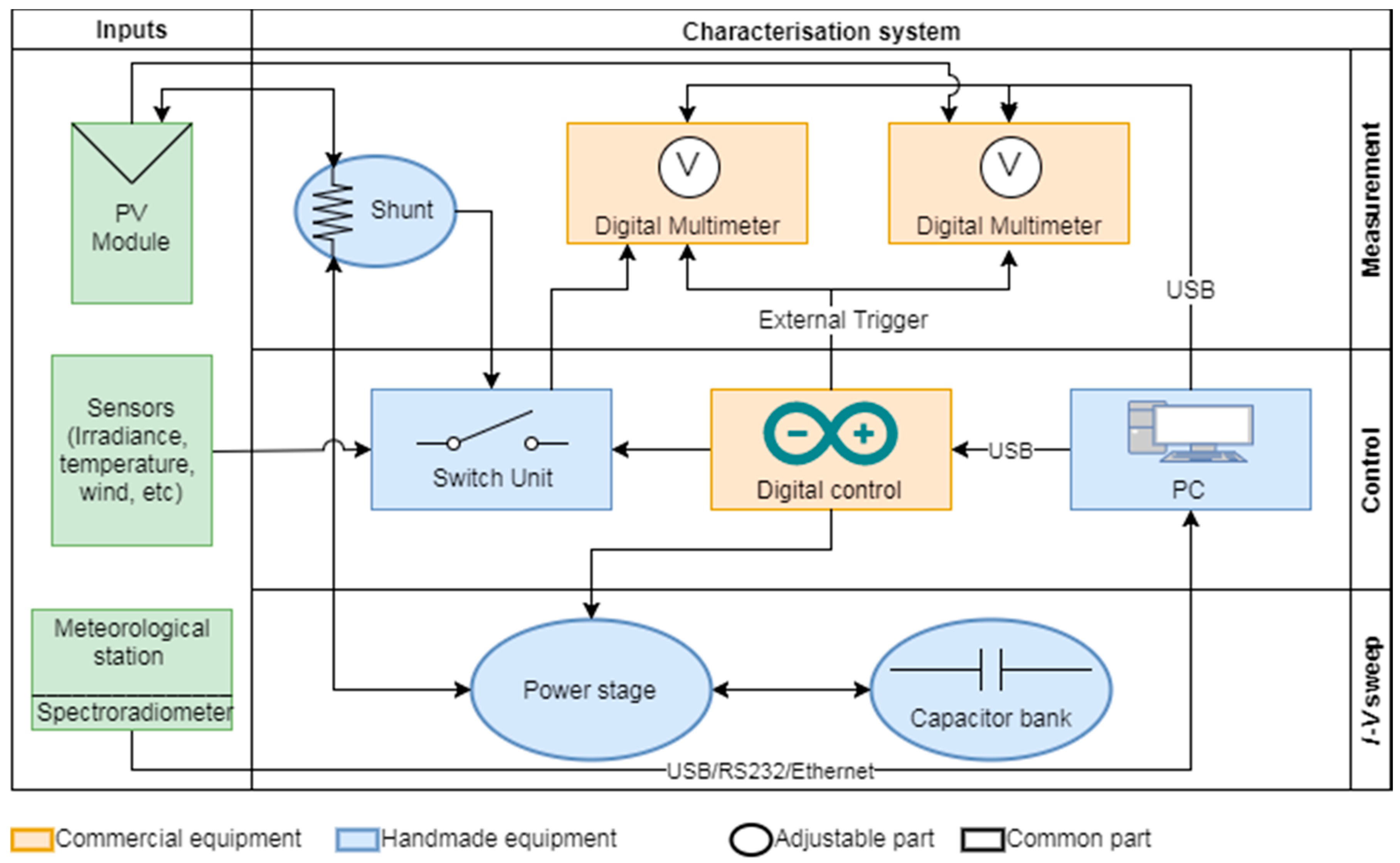
The proposed characterization system consists on an open platform employed according to the schematic diagram exhibited in Figure 1. This system consists of three blocks: I-V sweep, measurement, and control.

The I-V sweep block is an electronic system able to reproduce a variable impedance from zero to infinite in order to perform the I-V sweep of a PV module. Amongst all the available methods [18], this block is based on a capacitive load. Therefore, it includes a power stage and the capacitor bank. The power stage is a circuit board addressed to control the process of charge and discharge of the capacitor bank. This power stage was designed by the IDEA research group [29,30,31].

The measurement block includes specific instrumentation with calibration certificates, which delimits the error associated with the measurement and it is generated as a result of the periodic calibration. Any specific instrumentation can be used for this purpose. It only has to include a series of characteristics to be satisfactory: (a) communication to the PC through any kind of communication protocol; (b) the use of an external trigger to synchronize the voltage and current measurements; (c) enough buffer to store the measurement of each I-V curve; (d) enough sampling frequency to measure the desired number of points during the charge of the capacitor; and (e) the capacity of measuring different types of temperature sensors. Definitely, any mid- to top-range multimeter of any recognized brand can fulfill the necessary requirements. In the proposed set-up, the measurement block is composed off two Agilent 34411A multimeters to record the voltage and the current values simultaneously. One of them is used to measure the voltage across the terminals of the PV device. The second one is used to measure the current by means of the voltage drop across a shunt resistor between the device and the capacitor. In addition, the second multimeter also measures the operation conditions. Both multimeters are synchronized by a shared external trigger signal generated by the digital control system.

The control block carries out the management of the I-V sweep block and the synchronization, configuration, and communication of the measurement block. The control block is composed of a switch unit, a digital control, and a PC. As the second multimeter is used to measure several signals (including the voltage drop across the shunt resistor), a relay board that multiplexes the different signals is required. The digital control is responsible for generating the signals that control the power stage, synchronizing the measurements through the external trigger and controlling the switch unit that allows the measurement of several sensors. For this purpose, an Arduino board has been installed in the proposed experimental set-up. This board and both multimeters are connected to the PC by USB ports in order to be controlled by the application. Optionally, a meteorological station or a specific equipment, such as a spectroradiometer, can be connected directly to the PC by a standard communication port. The software, in our case programmed in LabVIEW, offers the flexibility of adding any number and type of sensors. It is also able to perform an automatic experimental measurement campaign where the obtained data are processed in real time. Another important feature is the centralization and synchronization of the data. Also, the obtained parameters are synchronized with the sweep of the I-V curve and recorded at the same time. Since the complete system is open, it can be modified to implement new data treatment techniques on each measured I-V curve that may emerge in future researches.

Most of the equipment included is common and independent of the size of the photovoltaic device to be characterized. The common part of the system includes both multimeters, the switch unit, the digital control board, and the PC with the control software. However, other parts of the system, such as the capacitor bank, the shunt resistor, and the power stage, must be designed and replaced depending on the specifications of the PV generator in terms of maximum current and voltage. In this way, the I-V curve tracer can be scaled to measure from a single cell to a power plant generator by selecting a suitable power stage, shunt resistor, and capacitor bank.

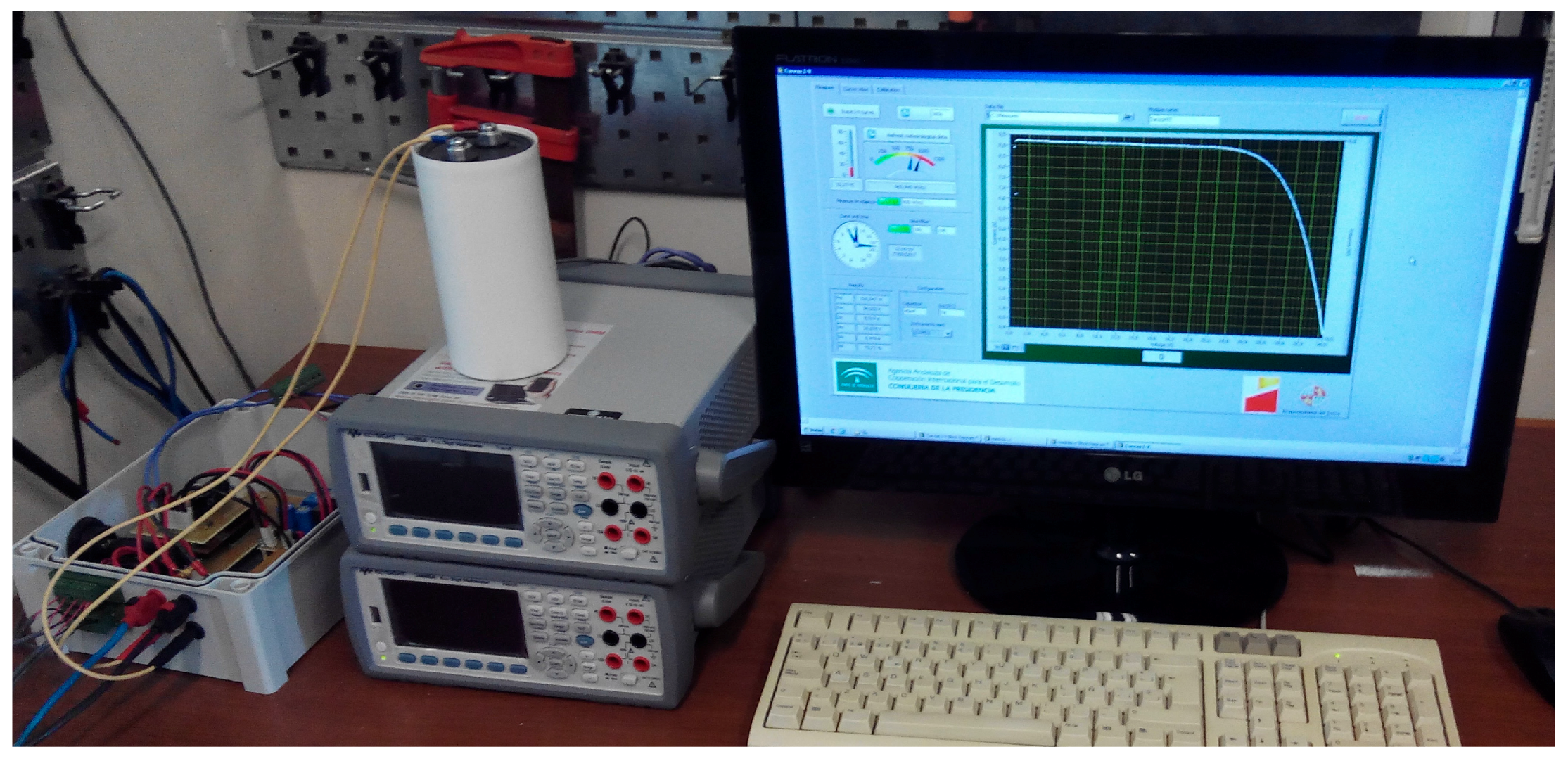
In Figure 2, an image of the system employed to perform the experimental campaign of measurement is exposed.

3.2. Hardware Description and Design

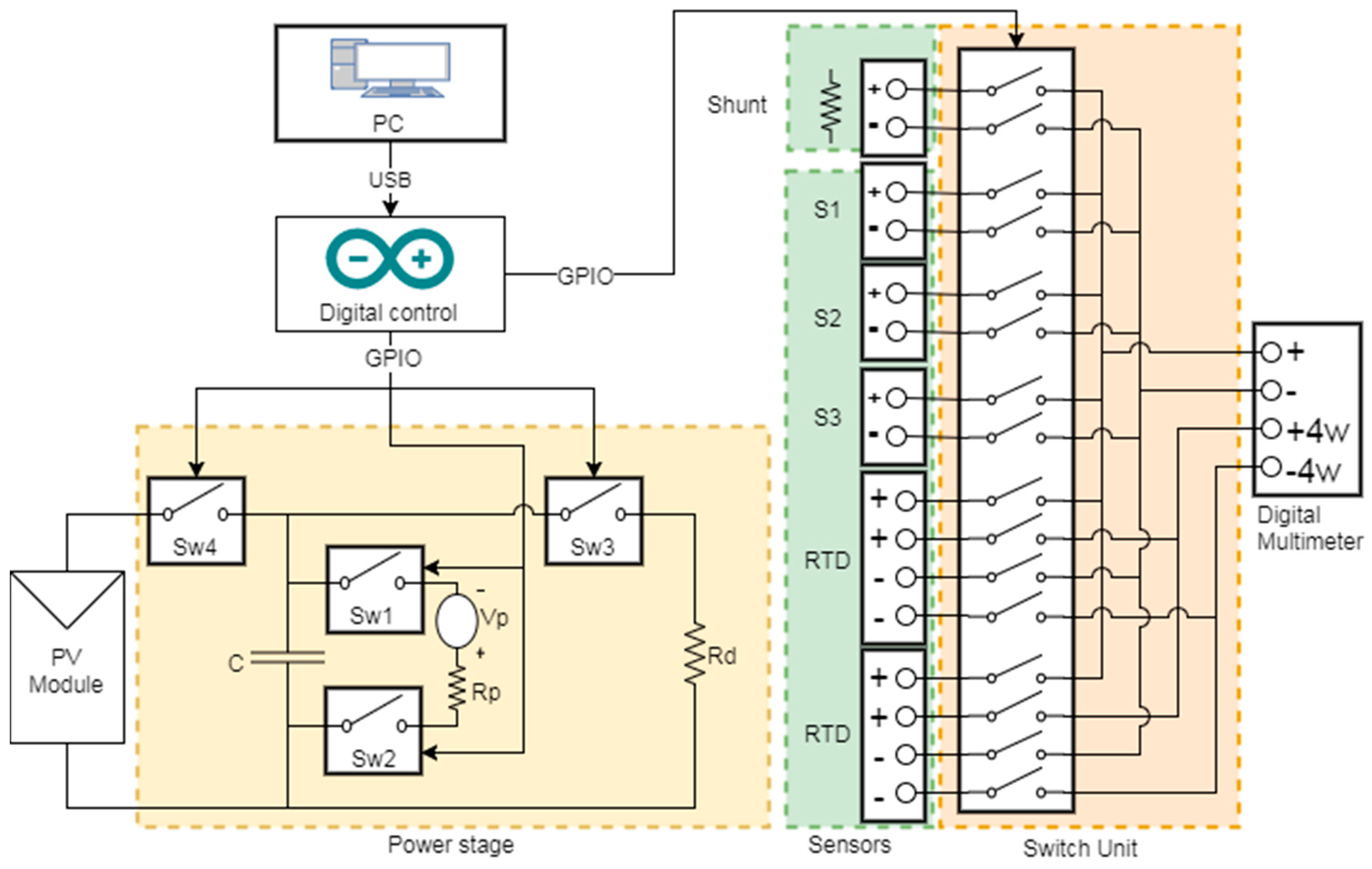
In Figure 3, the schematic of the hand-made equipment and its connections are presented. As was mentioned previously, the power stage controls the charge and discharge process of the capacitor bank. Three procedures are required—in this order—to plot the I-V curve: pre-charge, charge, and discharge. The pre-charge process negatively charges the capacitor bank to ensure that the PV device starts biased at the second quadrant (V < 0; I > 0) and the sweep passes through the short-circuit point during the charging process. The pre-charge voltage is set at 5 V, and it must be taken into account that high-reversed voltages at the capacitor may damage this component. Secondly, the charge process sweeps the I-V curve of the PV device during the charging time of the capacitor. The measurements of current and voltage of the PV device must be taken during this process to obtain the I-V curve. Finally, the capacitor must be discharged. To achieve this process, the stored energy at the capacitor is consumed by a power resistor.

In order to control the mentioned process, four switches—labelled as Sw1, Sw2, Sw3, and Sw4—are used. Switches Sw1 and Sw2 regulate the connection of the pre-charge source labelled as Vp. To avoid a short circuit at the pre-charge source at the beginning of this process, a resistor R_p is introduced. Sw3 switch governs the discharge procedure of the capacitor bank through the resistor R_d. Finally, the most critical element of this circuit is the switch Sw4, which is addressed to connect and disconnect the photovoltaic device to the capacitor bank.

The switches must be selected according to the PV device under test: the maximum voltage provided by the PV generator must be tolerated by all switches. Switch Sw4 must also allow the maximum current generated by the PV device, and it is also recommended to have a low serial resistance value. Therefore, technologies such as SCR, IGBT, or MOSFET are the most suitable for this task. Switches Sw1 and Sw2 should allow the current provided by the pre-charge source. Finally, switch Sw3 must tolerate the discharge current, which depends on the resistor R_d. All the control signals used to trigger the switches are generated by the digital control board and commanded by the LabVIEW application.

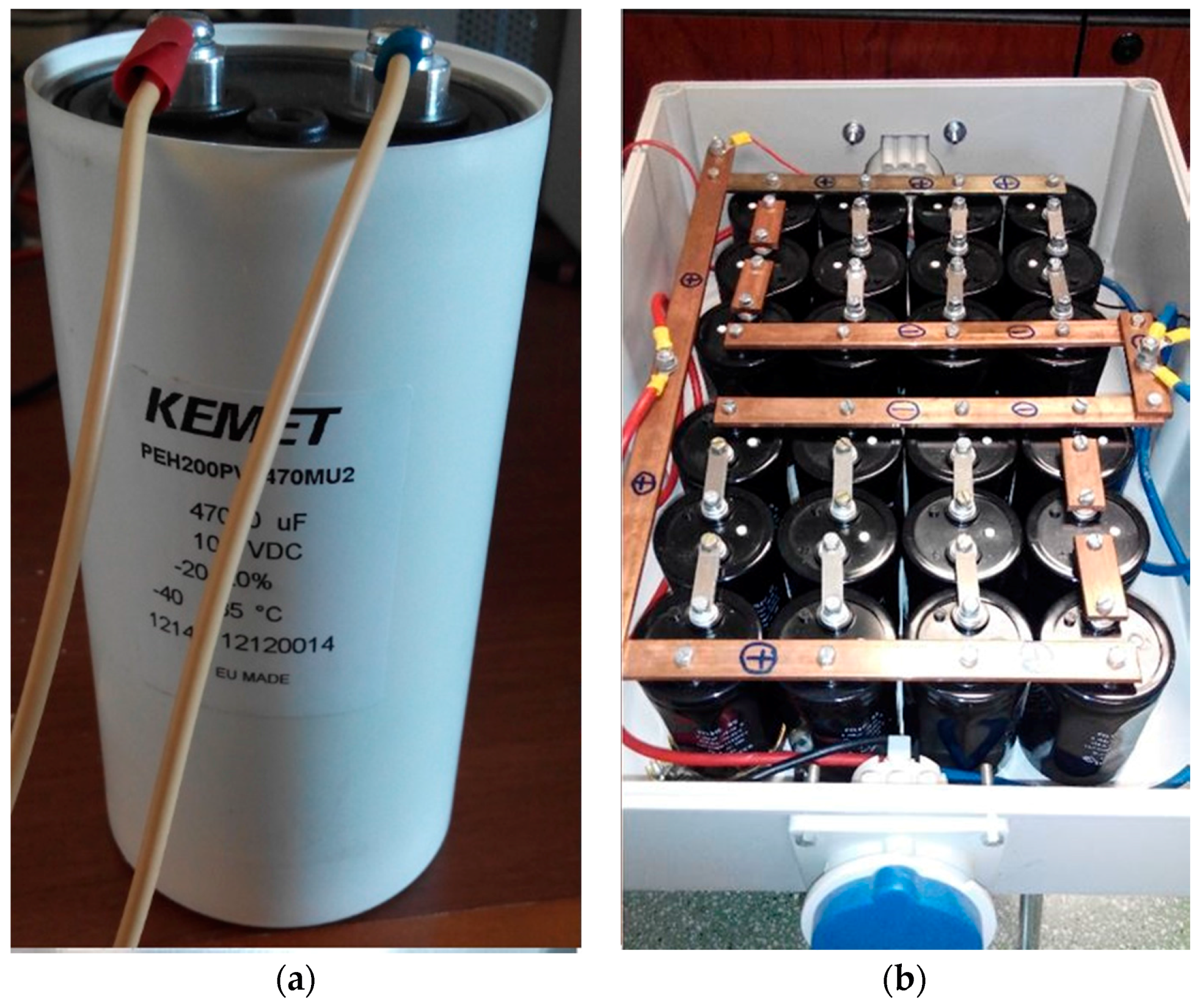
The design of the capacitor bank—labelled as C inside the power stage—must have a maximum permissible voltage superior to the voltage of the PV generator. For example, the capacitor bank shown in Figure 4a was employed to measure a single module up to 100 V. A capacitor bank—composed by 24 capacitors—that can perform the I-V curve of a 900 V PV generator is also shown in Figure 4b. 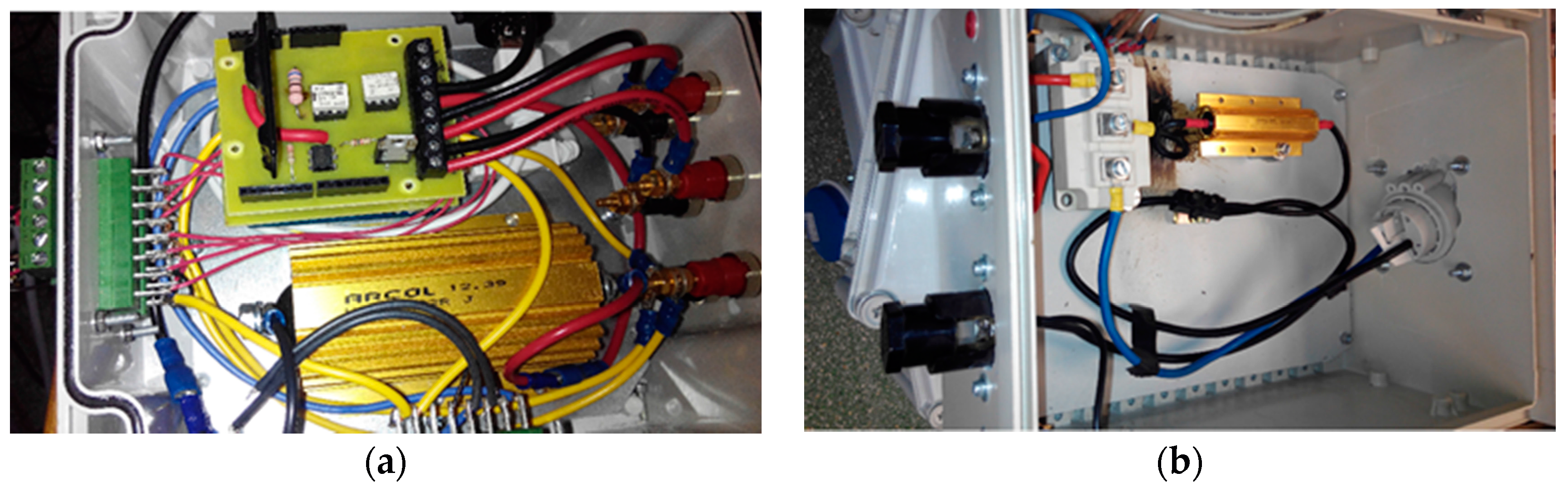The capacitance of the capacitor bank has to be selected to fit in the desired charging time range [35], which is delimited by the multimeters integration time. The charging time depends on the capacitance of the capacitor bank and the voltage and current provided by the PV generator. The integration time is a configurable parameter of the multimeters that adjusts the required time to perform a single measure. Therefore, the integration time is set depending on the number of points to capture and the required time to charge the capacitor bank. In the same way, the value of the discharging resistor influences the time that is necessary to discharge the capacitor. The maximum power dissipation of the discharge resistor must be also considered. A balance between the discharge time and the power dissipation should be sought. Different implementations of the power stage are shown in Figure 5. They were used for several tests depending on the power (voltage and current) of the PV device. In Figure 5a, a PV module power stage design is presented. This design is based on an SCR to control the charging process of the capacitor, low power relays to perform the negative pre-charge of the capacitor, and a solid state relay to control the discharge of the capacitor process. This power stage design has been used to measure PV modules up to 400 Wp. In Figure 5b, a large PV generator power stage is shown. This design is based on IGBG technology and allows the measurement of high power PV generators from 20 kWp to 200 kWp.

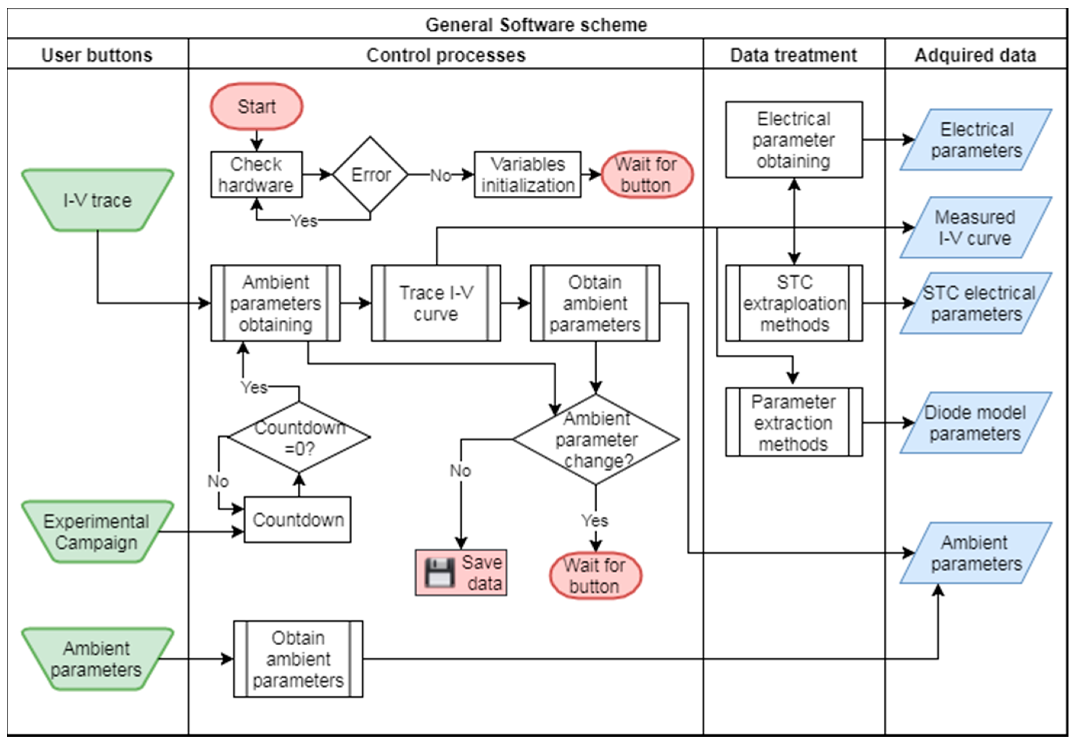
3.3. Control, Processing, and Storing Software

A personal computer is necessary to control the Arduino board and to process the measurements performed by the multimeters. The Arduino board and multimeters are connected to the PC by USB ports, so the PC must count with at least three USB ports. The use of this port—widely present on the PC market—rather than other ports such as GPIB or PXI makes the experimental set-up more suitable for laboratories with a reduced budget. As was mentioned before, a software application developed using LabVIEW from National Instruments [36] will run in the computer. The general schematic is presented in Figure 6, in which the principal control processes are activated by three user buttons. The main function of this software is to control the acquisition of the I-V curve and perform campaigns of measurements automatically. A campaign of measurements will be carried out, as this program can be easily configured to manage different PV devices—and consequently, different capacitors banks. The application is capable of processing measurements to obtain the main electrical parameters of the PV device (I_SC, V_OC, P_max, current at the maximum power point (IP_max), voltage at the maximum power point (VP_max) and FF), extrapolating them to STC using different methods [37,38,39,40], and extracting different intrinsic parameters from the single-diode model (photo-generated current (I_ph), saturation current (I₀), serial resistance (R_s), ideality factor (m), parallel resistance (R_sh)) using the methods described in [41,42,43]. All the acquired data are shown on screen and saved when the I-V curve is validated, that is, when the ambient parameters have no significant differences before and after the trace of the curve.

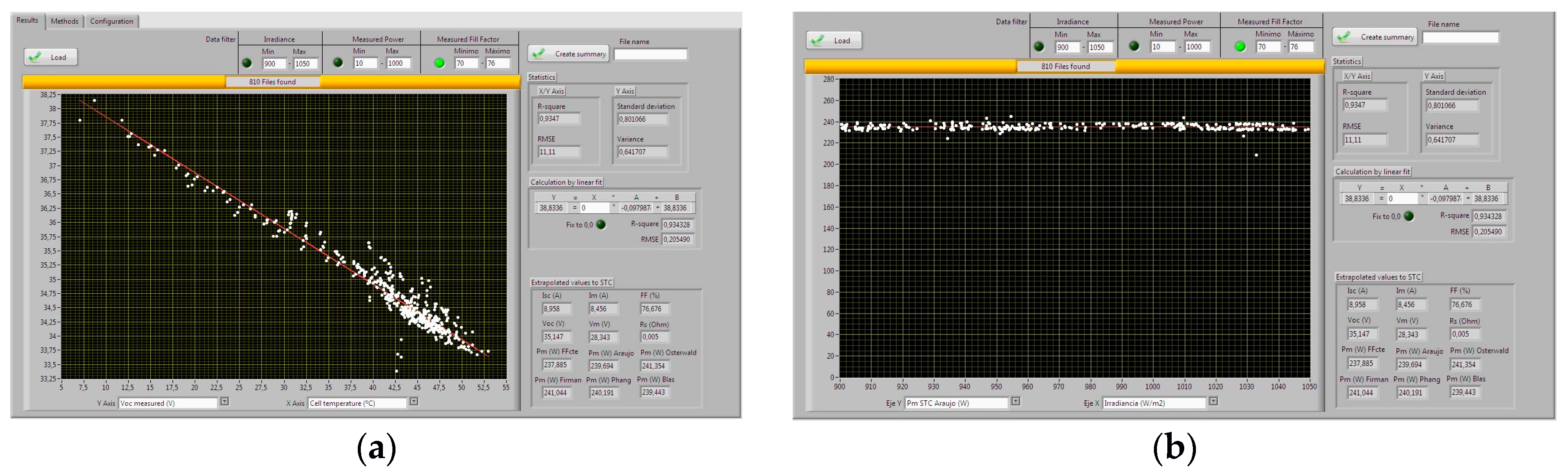
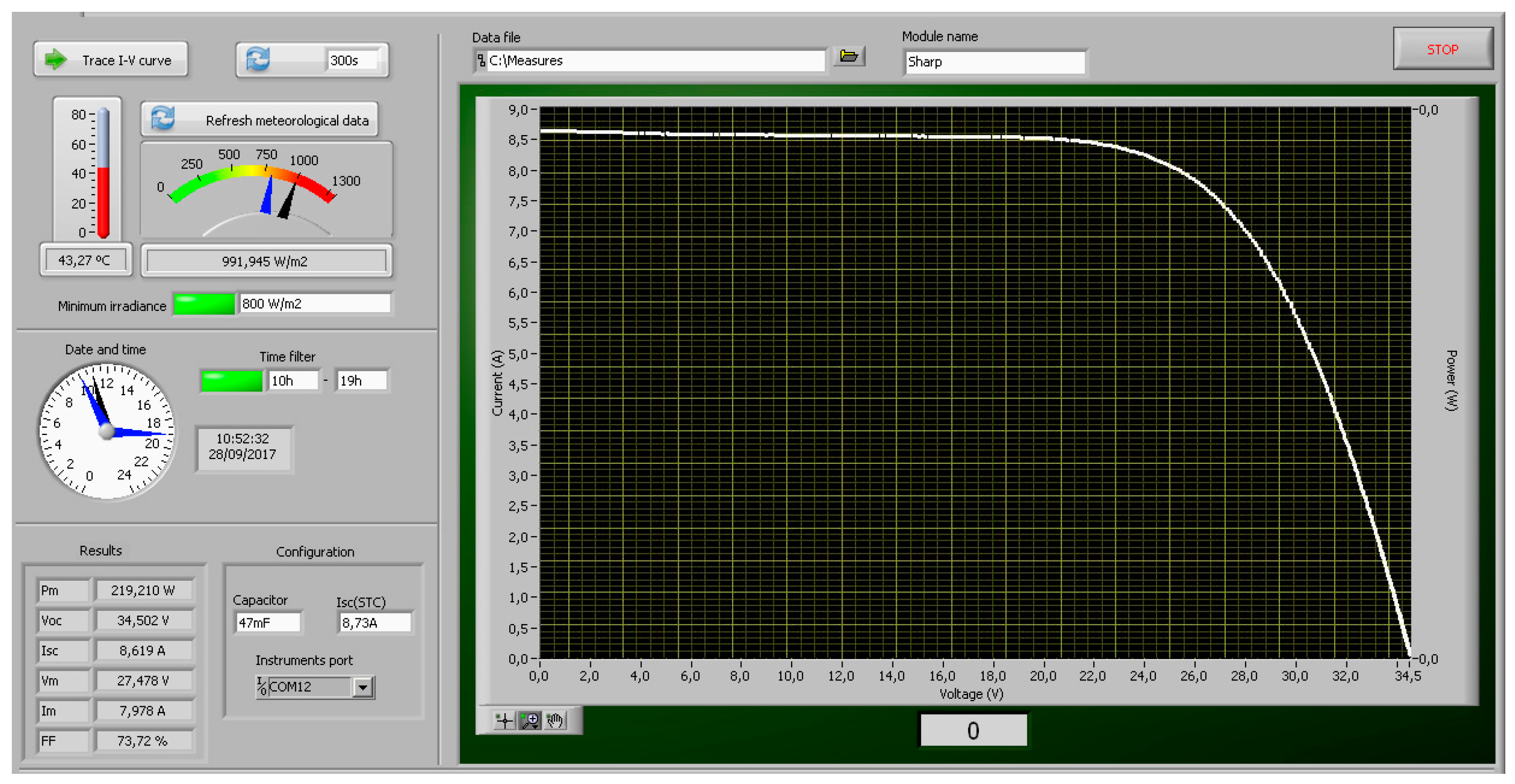
In Figure 7, a screenshot of the user panel from the implemented application is shown. The resulting I-V curve of a PV module under specific ambient conditions is displayed on the screen after performing a voltage sweep. Another remarkable feature of the software application is the possibility to perform—from among the data previously collected—charts where the variables to plot can be chosen by the user. Thus, the application allows the variable for abscissa and ordinate to be selected, which is a valuable characteristic for researchers and students [44] due to the fact that it makes feasible correlations between recorded variables. For example, in Figure 8a, the dependency on the temperature for the open circuit voltage of the PV module is shown. 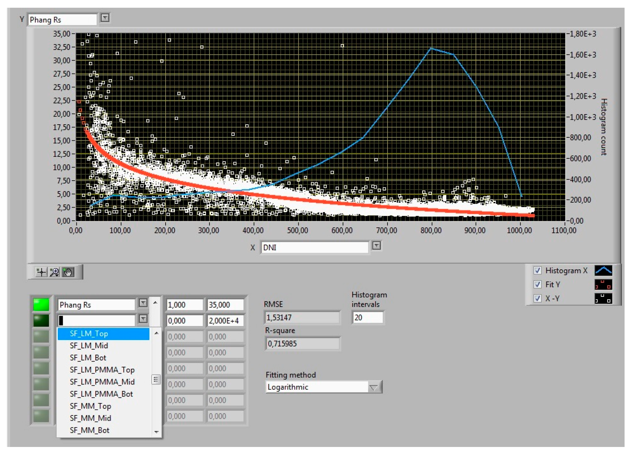Other plots can represent the STC values obtained in comparison with any parameter as they are presented in Figure 8b. Also, linear fits can be done between the represented variables and provide some statistical parameters, such as the standard deviation, variance, coefficient of determination, or root mean square deviation. The representation of the extracted parameters from the single diode model can also be represented in the function of the other parameters, as can be seen in Figure 9. Filters of all parameters can be implemented in the plots.

4. Estimation of Uncertainty

All measurement equipment must display the results providing a value of the measured magnitude and an estimation of its uncertainty. The measurement system proposed in this paper is based on a pair of multimeters with their respective calibration certificates from the manufacturer. Thus, an uncertainty study for the obtained results can be easily performed. An estimation of the inherent uncertainty associated with the multimeter is provided in the first part of this section. Furthermore, these uncertainties can be combined in order to determine the uncertainty associated with the I-V pairs and will be explained in the second part of this section. The third part explains how the uncertainty of the main electrical parameters: short-circuit current I_SC, open circuit voltage V_OC, maximum power P_max, and fill factor FF, is calculated. Finally, those expressions are put into practice for a commercial module measured at three different irradiance levels, giving for each example curve the uncertainty associated with the main electrical parameters.

This uncertainty analysis is based on concepts defined in the guide JCGM GUM [45]. In the literature, there are some works where an analogous analysis has been applied to determine the uncertainty of measurement systems in the field of photovoltaic systems [19,46].

4.1. Uncertainty Associated to the Multimeter

All the measurements are performed by the Agilent 34411A [47]. There are three sources of uncertainty associated with this instrument: accuracy (A), resolution (B), and calibration standard (C).

The uncertainty due to the accuracy depends on the selected measurement range; for this analysis, the PV device to be characterized has been assumed to have, at most, 100 V of open-circuit voltage and 10 A of short-circuit current to fit into the worst case possible for the PV device used.

The accuracy of the multimeter can be computed as the addition of two terms: a percentage of the measured value and another percentage of the selected range:

$$A=\left(\%\mathrm{reading}\right)\times \left(\mathrm{outputvalue}\right)+\left(\%\mathrm{range}\right)\times \left(\mathrm{selected}\mathrm{range}\right)$$

(1)

where the (% reading) and (% range) to apply are provided by the manufacturer as a table of coefficients (see

Table 1. Accuracy coefficients for an Agilent 34411A multimeter (% of reading + % of range).

	Range	Integration Time	Column 1	Column 2	Column 3	Column 4
Module Voltage	100 V	0.02 PLCs	0.0040 + 0.0006	0.0005 + 0.0001	0.0 + 0.0030	0.0 + 0.0003
Module Current	1 V	0.02 PLCs	0.0035 + 0.0007	0.0005 + 0.0001	0.0 + 0.0030	0.0 + 0.0003

, Column 1).

Mainly, there are two types of measurement: voltage component of each I-V point, and the current component of each one measured through a shunt resistor. The values given in Column 1 must be incremented if the temperature of the multimeters is beyond a specific range. For each additional degree outside the range [18 °C, 28 °C], the value in Column 1 should be incremented by the value in Column 2. Finally, another additional term should be added if the integration time is set to a value different to 100 Power Line Cycles (PLC). The integration time used to capture the current-voltage pairs of the I-V curve will be 0.02 PLCs. Due to the integration time, the noise adder term can be seen in Table 1, Column 3. Several cases will be considered, and thus different expressions of the uncertainty will be obtained according to the accuracy with which measurements were recorder. Another source of uncertainty comes from the resolution of analog to digital conversion, so the last parameter is given in Column 4.

$$A_V(\mathrm{V})=0.00009\left|V\right|+0.0046$$

(2)

$$A_{V_S}(\mathrm{V})=0.000085V_S+0.000047$$

(3)

where A_V is the uncertainty due to accuracy of a measurement V of the voltage between the terminals of the PV device and $A_{V_S}$ is the uncertainty associated with the reading of the voltage drop across the shunt used to measure the current by the PV device.

The uncertainty associated with the resolution can be estimated as one-half of the resolution given in Table 1, Column 4. Therefore, the values of uncertainty B due to resolution are: B_V = 0.00015 V for the module voltage and $B_{V_S}$ = 0.0000015 V for voltage drop in the shunt.

The third source of uncertainty is associated with the calibration standard used to calibrate the Agilent 34411A. The calibration certificate states that the multimeter was calibrated using a multimeter Fluke 5720A. On the Service Manual [48] of this second multimeter, the absolute uncertainty (with a 95% confidence level and k = 2) is provided giving two parameters, a ppm of the reading and an offset value (see

Table 2. Absolute uncertainties of Fluke 5720A (95% confidence level, k = 2).

	Calibrated Value	Fluke 5720A Range	Absolute Calibration Uncertainty
			ppm × Reading	+ offset
Module Voltage	100 V	220 V	5 ppm	40 μV
Module Current	1 V	2.2 V	5 ppm	0.7 μV

). For each case of measurement, this uncertainty could be calculated as follows in the Equation (4):

$$C=\left(\mathrm{ppm}\mathrm{of}\mathrm{reading}\right)\times \left(\mathrm{calibrated}\mathrm{value}\right)+\left(\mathrm{offset}\right)$$

(4)

Performing the required calculations, the obtained uncertainty is C_V = 0.00054 V (module voltage) and = 0.0000057 V (voltage drop in the shunt resistor).

The acquired uncertainties for module voltage and current will have a confidence level of 95% with k = 2. To obtain the standard uncertainty of resolution and accuracy, both terms are divided by $\sqrt{3}$ due to the fact that nothing is known about the error distribution. The calibration uncertainty is provided by Fluke—with a 95% of confidence level and coverage factor k = 2, which implies a normal distribution of the error—and to compute the standard uncertainty, the value C should be divided by 2. Then, the combined uncertainty of a measurement of module voltage using Agilent 34411A can be computed using the following expression:

$$U_V(\mathrm{V})=2\sqrt{{\left(\frac{A_V}{\sqrt{3}}\right)}^2+{\left(\frac{B_V}{\sqrt{3}}\right)}^2+{\left(\frac{C_V}{2}\right)}^2}=2\sqrt{2.7\times {10}^{-9}{V}^2+2.8\times {10}^{-7}\left|V\right|+7.1\times {10}^{-6}}$$

(5)

In case of the measurement of the module current, there is another source of uncertainty related to the quality of the shunt resistor itself. For the experimental setup, the shunt class is 0.5. This means that it could be a maximum error of 0.5% of the measured value:

$$E_S=0.5\%\cdot V_S=0.005\cdot V_S$$

(6)

Again, nothing should be supposed about the distribution associated with E_S, so this error must be divided by $\sqrt{3}$ to get the standard uncertainty. The combined uncertainty for the current measurement is given by:

$$\begin{array}{cc}\hfill U_{V_S}\left(V\right)& =2\sqrt{{\left(\frac{A_{V_S}}{\sqrt{3}}\right)}^2+{\left(\frac{B_{V_S}}{\sqrt{3}}\right)}^2+{\left(\frac{C_{V_S}}{2}\right)}^2+{\left(\frac{E_S}{\sqrt{3}}\right)}^2}\hfill \\ & =2\sqrt{8.3\cdot {10}^{-6}{V}_{S^2}+2.7\cdot {10}^{-9}{V}_S+7.5\cdot {10}^{-10}}\hfill \end{array}$$

(7)

In fact, $U_{V_S}$ is the uncertainty of the voltage measurement from the shunt resistor. The current value should be computed by the shunt specification: 10 A/150 mV. Therefore, the uncertainty expressed in amperes will be:

$$U_I\left(A\right)=\frac{10A}{150\mathrm{mV}}\cdot U_{V_S}=2\sqrt{8.3\cdot {10}^{-6}{I}^2+1.8\cdot {10}^{-7}I+3.3\cdot {10}^{-6}}$$

(8)

For each current-voltage point of the I-V curve, the value of power is calculated as P = VI. According to Piliougine et al. [14], the uncertainty of a calculated value can be estimated by propagating the uncertainties using the partial derivatives of the formula of the power. Hence, the expanded uncertainty of the power value of each point of the curve can be calculated by:

$$\begin{array}{c}{U}_P\left(W\right)=2\sqrt{{\left(\frac{\mathrm{dP}}{\mathrm{dV}}\right)}^2{\left(\frac{U_V}{2}\right)}^2+{\left(\frac{\mathrm{dP}}{\mathrm{dI}}\right)}^2{\left(\frac{U_I}{2}\right)}^2}=2\sqrt{I^2\cdot {\left(\frac{U_V}{2}\right)}^2+V^2\cdot {\left(\frac{U_I}{2}\right)}^2}\hfill \\ =2\sqrt{8.3\cdot {10}^{-6}{V}^2{I}^2+2.8\cdot {10}^{-7}\left|V\right|I^2+7.1\cdot {10}^{-6}{I}^2+1.8\cdot {10}^{-7}{V}^{2}I+3.3\cdot {10}^{-6}{V}^2}\hfill \end{array}$$

(9)

4.2. Uncertainty of the Main Electrical Parameters

In order to calculate the short circuit current I_SC, the linear interpolation of the point immediately before the zero voltage axis (V₀, I₀) and the point immediately after it (V₁, I₁) should be done. Therefore, I_SC can be estimated using the following expression:

$$I_{\mathrm{SC}}=I_1-V_1\frac{I_1-I_0}{V_1-V_0}$$

(10)

The Equation (10) used to calculate I_SC has its own uncertainties that should be propagated to estimate the uncertainty of I_SC using this formula:

$$\begin{array}{c}{U}_{I_{\mathrm{SC}}}=2\sqrt{{\left(\frac{d{I}_{\mathrm{SC}}}{d{V}_0}\right)}^2{\left(\frac{U_{V_0}}{2}\right)}^2+{\left(\frac{d{I}_{\mathrm{SC}}}{d{I}_0}\right)}^2{\left(\frac{U_{I_0}}{2}\right)}^2+{\left(\frac{d{I}_{\mathrm{SC}}}{d{V}_1}\right)}^2{\left(\frac{U_{V_1}}{2}\right)}^2+{\left(\frac{d{I}_{\mathrm{SC}}}{d{I}_1}\right)}^2{\left(\frac{U_{I_1}}{2}\right)}^2}\\ =2\sqrt{{\left(\frac{V_1\left(I_1-I_0\right)}{{\left(V_1-V_0\right)}^2}\right)}^2{\left(\frac{U_{V_0}}{2}\right)}^2+{\left(\frac{V_1}{V_1-V_0}\right)}^2{\left(\frac{U_{I_0}}{2}\right)}^2+{\left(\frac{V_0\left(I_1-I_0\right)}{{\left(V_1-V_0\right)}^2}\right)}^2{\left(\frac{U_{V_1}}{2}\right)}^2+{\left(\frac{V_0}{V_1-V_0}\right)}^2{\left(\frac{U_{I_1}}{2}\right)}^2}\end{array}$$

(11)

In addition, to estimate V_OC, the set of points {(V_k, I_k)|I_k < U_I (0)} must be taken into account, where U_I (0) is the uncertainty of a current measurement equal to zero amperes. The estimated value of V_OC can be calculated as the mean value of all the points in that set. The standard uncertainty is computed as the standard deviation of the voltage values around that mean value. Therefore, the value of V_OC and its expanded uncertainty due to the approximation procedure can be estimated using the following expressions:

$$V_{\mathrm{OC}}\left(V\right)=\frac{1}{n}{\displaystyle \sum }_{k=1}^n{V}_k$$

(12)

$$U_{I\approx 0}\left(V\right)=2\sqrt{\frac{1}{n-1}{\displaystyle \sum }_{k=1}^n{\left(V_k-V_{\mathrm{OC}}\right)}^2}$$

(13)

where n is the number of points of the set.

In addition, the last voltage uncertainty due to the approximation procedure must be combined to the uncertainty due to a single measurement of voltage around the calculated value of V_OC:

$$U_{V_{\mathrm{OC}}}=2\sqrt{{\left(\frac{U_V\left(V_{\mathrm{OC}}\right)}{2}\right)}^2+{\left(\frac{U_{I\approx 0}}{2}\right)}^2}$$

(14)

The maximum power P_max is computed as maximum value of V_k·I_k among all discrete points of the curve, but this is an underestimation of the actual value of P_max, and hence an additional source of uncertainty is added. This uncertainty can be neglected if there is a high density of points around the knee of the curve, as stated in [19]. This fact can be ensured if the difference in power between two consecutive points is much less than the uncertainty in power of a single point: |P_i+1 − P_i| <<< U_P (P_i). For example, in the checked case |P_i+1 − P_i| < 0.2 U_P (P_i), and if the last expression is not satisfied, the I-V curve should be discarded and the speed of the multimeters should be increased to acquire more points at the same time. Therefore, the uncertainty of the value of P_max will be the uncertainty in power of a single measured point provided by the next equation:

$$\begin{gathered} U_{P_{max}}(\mathrm{W})=2\sqrt{I{P}_{max}^2\cdot {\left(\frac{U_{V{P}_{max}^{}}}{2}\right)}^2+V{P}_{max}^2\cdot {\left(\frac{U_{I{P}_{max}^{}}}{2}\right)}^2}= \\ =2\sqrt{8.3\cdot {10}^{-6}V{P}_{max}^{2}I{P}_{max}^2+1.8\cdot {10}^{-7}V{P}_{max}^2{I}_{P_{max}}^{}2.8\cdot {10}^{-7}V{P}_{max}^{}I{P}_{max}^2+3.3\cdot {10}^{-6}V{P}_{max}^2+7.1\cdot {10}^{-6}I{P}_{max}^2} \end{gathered}$$

(15)

Finally, for each measured I-V curve, its fill factor will be computed using the following expression:

$$\mathrm{FF}=\frac{P_{max}}{I_{\mathrm{SC}}\cdot V_{\mathrm{OC}}}=\frac{{\mathrm{IP}}_{max}\cdot {\mathrm{VP}}_{max}}{I_{\mathrm{SC}}\cdot V_{\mathrm{OC}}}$$

(16)

Therefore, the uncertainty associated to each value of FF can be computed as:

$$\begin{gathered} U_{FF}=2\sqrt{{\left(\frac{dFF}{d{P}_{max}}\right)}^2\cdot {\left(\frac{U_{P_{max}}}{2}\right)}^2+{\left(\frac{dFF}{d{I}_{\mathrm{SC}}}\right)}^2{\left(\frac{U_{I_{\mathrm{SC}}}}{2}\right)}^2+{\left(\frac{dFF}{d{V}_{\mathrm{OC}}}\right)}^2{\left(\frac{U_{V_{\mathrm{OC}}}}{2}\right)}^2}= \\ =2\frac{1}{I_{\mathrm{SC}}\cdot V_{\mathrm{OC}}}\sqrt{{\left(\frac{U_{P_{max}}}{2}\right)}^2+\frac{P_{max}^2}{I_{\mathrm{SC}}^2}{\left(\frac{U_{I_{\mathrm{SC}}}}{2}\right)}^2+\frac{P_{max}^2}{V_{\mathrm{OC}}^2}{\left(\frac{U_{V_{\mathrm{OC}}}}{2}\right)}^2} \end{gathered}$$

(17)

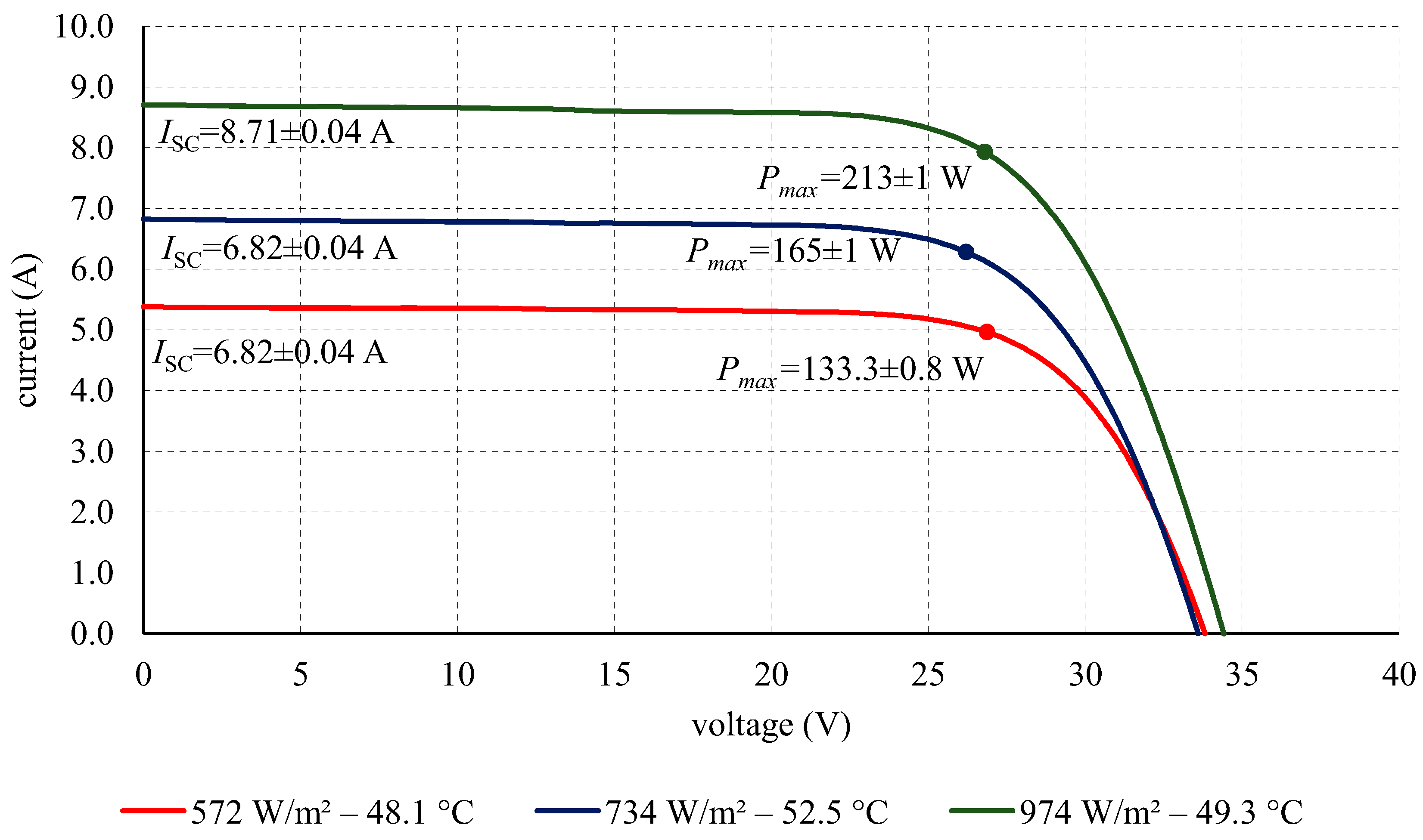
4.3. Practical Case of Uncertainty Estimation

In order to illustrate the practical use of the expressions previously described, three examples of I-V curves under different weather conditions are measured for a commercial photovoltaic module Sharp NU245J5 and the results are exposed in Figure 10. In addition, the values of the irradiance G, the cell temperature T_c, the short circuit current I_SC, the open circuit voltage V_OC, the maximum power P_max, and the fill factor FF are obtained for each measured curve and their respective uncertainties are calculated accordingly to the set of expressions provided previously. The results are shown in

Table 3. Electrical parameters extracted from curves shown in Figure 9 for Sharp NU245J5 module.

	Curve 1	Curve 2	Curve 3
G (W/m2)	572 ± 24	734 ± 30	974 ± 40
Tm (°C)	48.1 ± 1.3	52.5 ± 1.3	52.5 ± 1.3
ISC (A)	5.38 ± 0.03	6.82 ± 0.04	8.71 ± 0.04
VOC (V)	33.81 ± 0.01	33.60 ± 0.01	34.41 ± 0.01
Pmax (W)	133.3 ± 0.8	165 ± 1	213 ± 1
FF (%)	73.3 ± 0.6	71.9 ± 0.6	70.9 ± 0.5

. Moreover, the specifications of the PV modules are shown in

Table 4. Specifications of the photovoltaic modules at STC.

	#1	#2	#3
Technology	mono-Si	multi-Si	HIT
Manufacturer	Sharp	Suntech	Sanyo
Model	NU245J5	STP-160	HIT-240HDE4
Num. of cells	60	72	60
Coeffcient α	+0.053%/°C	+0.06%/°C	+2.21 mA/°C
Coeffcient β	−130 mV/°C	−155 mV/°C	−109 mV/°C
Coeffcient γ	−0.485%/°C	−0.47%/°C	−0.30%/°C
Main Electrical Parameters at STC (Manufacturer)
ISC (A)	8.73	5.12	7.37
VOC (V)	37.5	42.4	43.6
Pmax (W)	245	160	240
IPmax (A)	8.04	4.78	6.77
VPmax (V)	30.5	33.5	35.5
Main Electrical Parameters at STC (IAL, Solar Simulator)
ISC (A)	8.68	5.03	7.45
VOC (V)	37.4	43.6	42.8
Pmax (W)	241	165	242
IPmax (A)	7.92	4.75	7.07
VPmax (V)	30.4	34.8	34.2
FF (%)	74.1	75.4	75.9

.

5. Experimental Design

The components that compose the experimental design and the methodology will be exposed in this section. Three commercial modules from different photovoltaic technologies—monocrystalline silicon, polycrystalline silicon and CIGS—have been characterized by measuring their I-V curves and computing their main electrical parameters. The modules and the necessary sensors for the experiment were located in an outdoor solar tracker placed on the terrace of the Engineering Building of the University of Jaen. The main electrical specifications in STC provided by the manufacturer are summarized in Table 4. In order to compare the obtained results to a true value, the modules were previously sent to an independent, accredited laboratory (IAL). The IAL (Centro de Investigaciones Energéticas, Medioambientales y Tecnológicas (CIEMAT), Madrid, Spain) performs characterizations under standard test conditions in a solar simulator. The electrical parameters given by the IAL are also exposed in Table 4. The system has been tested using a predetermined configuration suitable to measure a single commercial photovoltaic module. The selected configuration is summarized in

Table 5. Components used on the interchangeable part of the system.

Component	Manufacturer/Model	Characteristics
Capacitor bank	Kermet PEH200	V = 100 V
		C = 47 mF
Switch	TYN640	VDRM = 640 V
		IT = 40 A
Shunt	Kainos	I = 10 A
		V = 150 mV
Resistor	Arcol HS200	R = 22 Ω
		P = 200 W
Precharge source	Arduino	V = 5 V
		I = 50 mA

. In addition, the sensors connected to the system are shown in

Table 6. Sensors connected to the system.

Sensor	Manufacturer/Model	Parameter
Pyranometer	Kipp & Zonen CMP21	Global normal irradiance
Spectroradiometer	EKO MS-700	Solar spectrum
Platinum RTD	PT100	Cell temperature
Platinum RTD	PT100	Air temperature
Anemometer	Young 05305VM	Wind direction
Anemometer	Young 05305VM	Wind speed

. As an approximated budget of the system, the total material cost reached a value of $3000, while the value of two multimeters from the top range was approximately $2800, plus $200 of electronic material costs.

With the aim of quantifying the closeness of agreement of the proposed system, 50 curves per module have been selected under irradiance ranges between 950 W/m² and 1050 W/m². In order to compare the results obtained by the proposed system and the results given by the IAL, the I-V curves must be extrapolated into STC. For this, three extrapolation methods have been used. On the first hand, the model of Osterwald [39] is employed to estimate the value of P_max under STC for each measured curve. Besides, the method described by Araujo et al. [38] and the one published by Firman et al. [40] have been applied to determine also the value of I_SC, V_OC, and P_max at STC conditions; the FF is also computed using those parameters. In order to know the closeness of agreement between the measurements taken by experimental set-up and those ones recorded by the IAL, the RMSE (Equation (18)) and the relative error (Equation (19)) have been computed. It must be taken into account that the error is produced by the sum of two factors: the error generated from the measurement system and from the extrapolation method.

$$RMSE=\sqrt{\frac{1}{N}{\displaystyle \sum }_{i=1}^N\Re {\left(V\right)}_i^2}$$

(18)

$$\Re \left(V\right)=\frac{IALparameter-Measuredparameter}{IALparameter}$$

(19)

6. Results

The comparison between the obtained results by the proposed system and the results from an Independent Accredited Laboratory (IAL) will be exposed in this section. For each electrical parameter, the mean value, RMSE, and relative error of the set on STC from all the curves is computed and the results can be seen in

Table 7. Measurement of the CIEMAT vs. measurement of the proposed system over Sharp NU245J5.

	CIEMAT	Corrected to STC by Araújo			Corrected to STC by Firman			Corrected to STC by Osterwald
		MEAN	RMSE	Relative Error	MEAN	RMSE	Relative Error	MEAN	RMSE	Relative Error
ISC (A)	8.74	9.02	0.28	3.2%	9.02	0.29	3.3%
VOC (V)	37.4	37.57	0.20	0.5%	37.45	0.12	0.3%
Pmax (W)	241	236	5	2.1%	245	4	1.7%	249	9	3.6%
FF (%)	73.7	70.5	3.2	4.3%	72.6	1.2	1.7%

,

Table 8. Measurement of the CIEMAT vs. measurement of the proposed system over Suntech STP-160.

	CIEMAT	Corrected to STC by Araújo			Corrected to STC by Firman			Corrected to STC by Osterwald
		MEAN	RMSE	Relative Error	MEAN	RMSE	Relative Error	MEAN	RMSE	Relative Error
ISC (A)	5.03	5.26	0.23	4.6%	5.26	0.23	4.6%
VOC (V)	43.6	43.46	0.16	0.4%	43.52	0.21	0.5%
Pmax (W)	165	161	4	2.4%	168	3	1.8%	172	7	4.2%
FF (%)	75.4	71.4	4.0	5.3%	73.3	2.1	2.8%

and

Table 9. Measurement of the CIEMAT vs. measurement of the proposed system over Sanyo HIT240.

	CIEMAT	Corrected to STC by Araújo			Corrected to STC by Firman			Corrected to STC by Osterwald
		MEAN	RMSE	Relative Error	MEAN	RMSE	Relative Error	MEAN	RMSE	Relative Error
ISC (A)	7.45	7.42	0.04	0.5%	7.43	0.04	0.5%
VOC (V)	42.8	42.63	0.18	0.4%	42.63	0.18	0.5%
Pmax (W)	242	233	10	4.1%	236	6	2.5%	237	7	2.9%
FF (%)	75.9	74.4	1.9	2.5%	74.5	1.4	1.8%

, and in Table 8 and Table 9 for Sharp NU245J5, Suntech STP-160, and Sanyo HIT240, respectively.

After analyzing the parameters used for establishing the closeness of agreement between the measured system and the IAL, the worst results obtained correspond to FF, which were less than 5.3%. The FF is the most difficult parameter to predict for the selected STC methods, since its value is highly affected by the parasitic resistances (serial and shunt resistances), which depend on the ambient conditions. Low differences were found on this parameter between the value measured at real conditions and the value extrapolated to STC. In terms of the short circuit current, the relative error was slightly higher than 3% for the Sharp NU245J5 (mono-Si), around 4.6% for the SunTech STP-160 (multi-Si), and only 0.5% for the Sanyo HIT. The I_SC value extrapolation to STC is very sensitive to the irradiance sensor measure and a slightly different α value (for these specific modules). Also, the uncertainties produced by the shunt resistor can be a great source of error. The error in the estimation of the open circuit voltage is different in the three cases, but never greater than 0.5%. In contrast to the previous parameter, this value is mainly affected by the temperature value. The β value is also a source of error in the extrapolation to STC. A lower error value may be justified for the higher stability of this parameter in outdoor conditions. Regarding the maximum power, for the Sharp NU245J5 using models by Araújo or Firman, the error in power is around 2–2.1% and 1.7%, respectively, whereas the Osterwald’s method has an error of 3.6%. In the same way, for the module Suntech STP-160, the error using the Osterwald’s method is more than 4%, while the error of the Araújo’s model is 2.4% and the error the of Firman’s model is only 1.8%. However, in case of the Sanyo HIT module, the model of Araújo, with a relative error of 4.1%, behaves worse than the other two models (2.5% for the Firman’s model and 2.9% for the Osterwald model). Surprisingly, the method of Osterwald—which is employed only to estimate the maximum power value—obtained the highest error results.

7. Conclusions

A complete system to measure the I-V curves of any photovoltaic device has been implemented. The system is based on three principles: the use of general purpose instrumentation to perform the measurements, which ensures accuracy and precision; the use of open-hardware, which allows the reproduction of the system in any laboratory; and scalability, which measures any PV device. These characteristics also reduce the final budget of the system.

The hardware is composed of a common part, which can be used to measure any PV generator, and an interchangeable part, which must be designed taking into account the specifications of the PV device under test. This way, the proposed system can be used to measure any PV generator. The provided software allows the process of measurement to be configured and controlled to automatically take I-V curves at regular intervals of time. In addition, the program offers a set of tools to perform data processing from the obtained I-V curves such as extrapolation to STC.

A deep study of the uncertainties associated with the measuring process was done. Thus, the reported I-V curves for the modules under test include their respective uncertainty.

A campaign of measurements was carried out. Three commercial modules of different photovoltaic technologies were characterized by the system. These modules were previously sent to an independent accredited laboratory in order to compare the results obtained by the proposed system to those given by the IAL. The obtained results prove that the relative error when measuring the main electrical parameters and performing the extrapolation to STC is less than 5%. In short-circuit the error is never greater than 5%, in open-circuit voltage is less than 0.5%, and in maximum power it is around 4% in the worst case. Thus, the obtained results suggest that the proposed system is suitable and can be profitable for laboratories with reduced budget or for educational applications.