Studies on Cup Anemometer Performances Carried out at IDR/UPM Institute. Past and Present Research

Abstract

In the present work, the research derived from a wide experience on cup anemometer calibration works at IDR/UPM Institute (Instituto Universitario de Microgravedad “Ignacio Da Riva”) is summarized. This research started in 2008, analyzing large series of calibrations, and is focused on two main aspects: (1) developing a procedure to predict the degradation level of these wind sensors when working on the field and (2) modeling cup anemometer performances. The wear and tear level of this sensor is evaluated studying the output signal and its main frequencies through Fourier analysis. The modeling of the cup anemometer performances is carried out analyzing first the cup aerodynamics. As a result of this process, carried out through several testing and analytical studies since 2010, a new analytical method has been developed. This methodology might represent an alternative to the classic approach used in the present standards of practice such as IEC 64000-12.

1. Introduction

Since 1997, the IDR/UPM Institute (Instituto Universitario de Microgravedad “Ignacio Da Riva”) has performed high level standardized calibrations to wind speed sensors, mainly for the wind energy sector and Spanish meteorology institutions. LAC-IDR/UPM is the calibration laboratory within this research institute, which is accredited according to ISO/IEC 17025 standard and is a member of the Measuring Network of Wind Energy Institutes (MEASNET) since 2003.

The line of work related to wind speed sensors calibration represents, together with space engineering [1,2,3,4,5,6,7,8,9,10,11], wind engineering [12,13,14,15,16,17], and different high education degree programs such as the Master in Space Systems [18,19,20,21], the core of the activities being carried out by the IDR/UPM research institute’s staff.

With regard to the aforementioned wind speed sensors calibration, this line of work has produced a strong research, mainly focused on cup anemometers (see Figure 1) [22,23,24,25,26,27,28,29,30,31,32,33,34]. Additionally, some relevant research devoted to sonic anemometers has been carried out at IDR/UPM [35,36,37,38,39]. Although other wind speed sensors such as the aforementioned sonic anemometer, LIDAR, SODAR, and nacelle anemometers, have been thoroughly developed and studied in order to substitute the cup anemometer along the past decades [40,41,42,43,44,45,46,47,48,49,50,51,52,53,54,55,56,57,58,59], this old fashioned but robust and reliable instrument (see Figure 1) developed by T.R. Robinson in the 19th century [60,61,62,63], remains the most demanded and used wind sensor for meteorologists and within the wind energy sector.

In addition, it should be pointed out that the demand of cup anemometers might increase, as the wind energy installed power has been continuously growing in the last years (see Figure 2). This fact also involves a huge demand for calibration of these sensors because any lack of accuracy in relation to the measured wind speed by an anemometer installed on a wind generator will have a major impact on the economic revenue (the extractable wind power is proportional to third power of the wind speed).

In this work, the research activities related to cup anemometer performance analysis carried out at IDR/UPM are reviewed. The work is organized as follows: the experimental analyses and results based on the huge calibrations database of the LAC-IDR/UPM are described in Section 2. In Section 3, the analytical models and procedures developed at IDR/UPM to study the cup anemometer are reviewed. Finally, conclusions are summarized in Section 4.

2. Experimental Analyses of Cup Anemometer Performances

Historically, the first analyses of cup anemometer performance were carried out based on experimental results, analyzing the performances [64,65,66,67] or searching for the optimum configuration (number of cups, size…) [68,69,70,71]. A thorough review of the literature was carried out in previous works [29,31].

In a first approach to anemometer performances, more than 3500 calibrations (performed at IDR/UPM on 25 different cup anemometer models) were studied by Pindado et al. [22]. The calibration of an anemometer involves the definition of its transfer function, which relates the measured wind speed, V, to the cup anemometer’s output frequency, f.

$$V=\mathrm{A}f+\mathrm{B}.$$

(1)

In the above equation, constants A (slope) and B (offset) are the ones that need to be defined by means of a proper calibration. However, it should be pointed out that normally the output frequency is not equal to the cup anemometer’s rotation frequency, f_r, due to the different electronic systems used to measure the rotation rate, which give a different number of pulses, m, along one turn of the rotor. Therefore, Equation (1) should be referred to f_r, in order to analyze the aerodynamic performances properly (obviously, A_r = m·A in the above equation).

$$V={\mathrm{A}}_r{f}_r+\mathrm{B}.$$

(2)

In Figure 3, the results of two different calibration procedures, performed on the same Thies 4.3350 cup anemometer, are shown. The first procedure, the AC calibration procedure, strictly follows MEASNET [72,73] requirements (13 measurement points taken within a wind speed bracket from 4 m·s⁻¹ to 16 m·s⁻¹), whereas the second one, the AD calibration procedure, is an internal procedure performed at the IDR/UPM Institute within a larger wind speed range and with less measurement points taken (nine measurement points taken within a wind speed bracket from 4 m·s⁻¹ to 23 m·s⁻¹). This AD calibration procedure was developed at customers’ request.

Two important conclusions were derived as a result of this work:

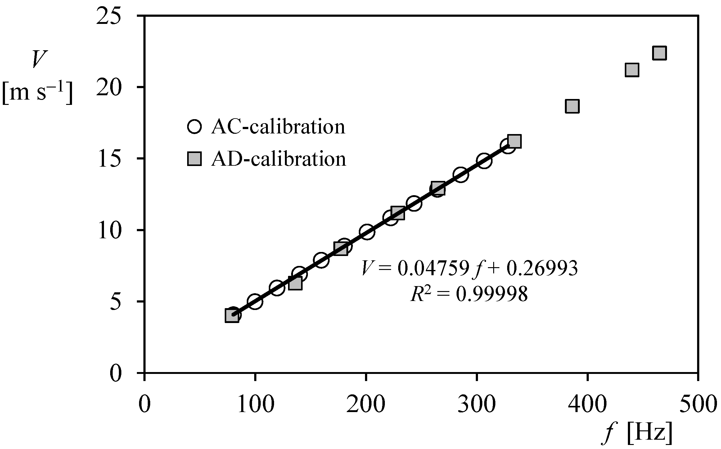
• The differences between the AC and AD calibration procedures were negligible in terms of both wind speed (with 2.6%, 0.88%, and 0.31% deviation at 5 m·s⁻¹, 10 m·s⁻¹, and 15 m·s⁻¹ wind speed for the Thies anemometer referred in Figure 3) and wind power generator Annual Energy Production (AEP);
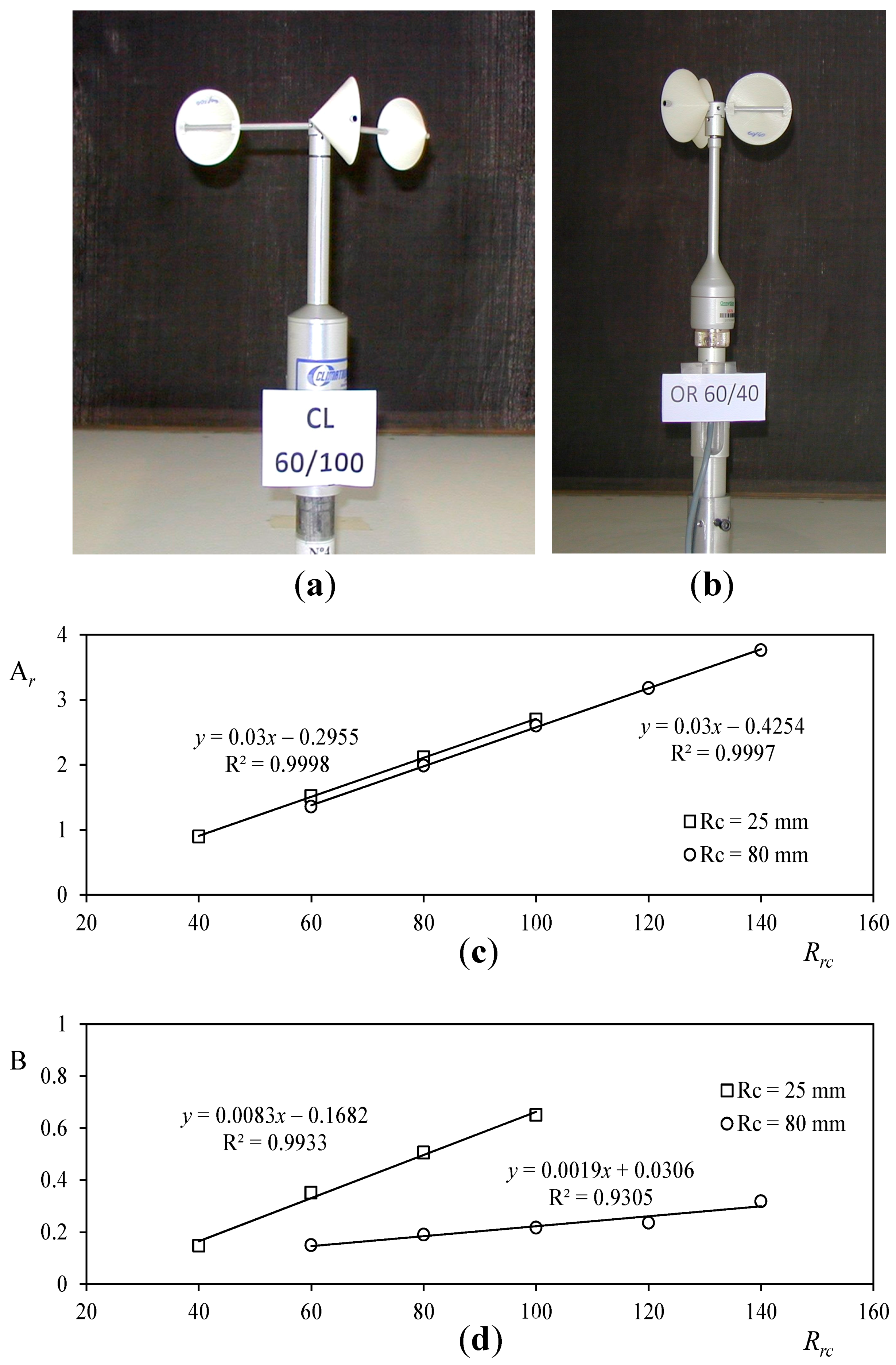
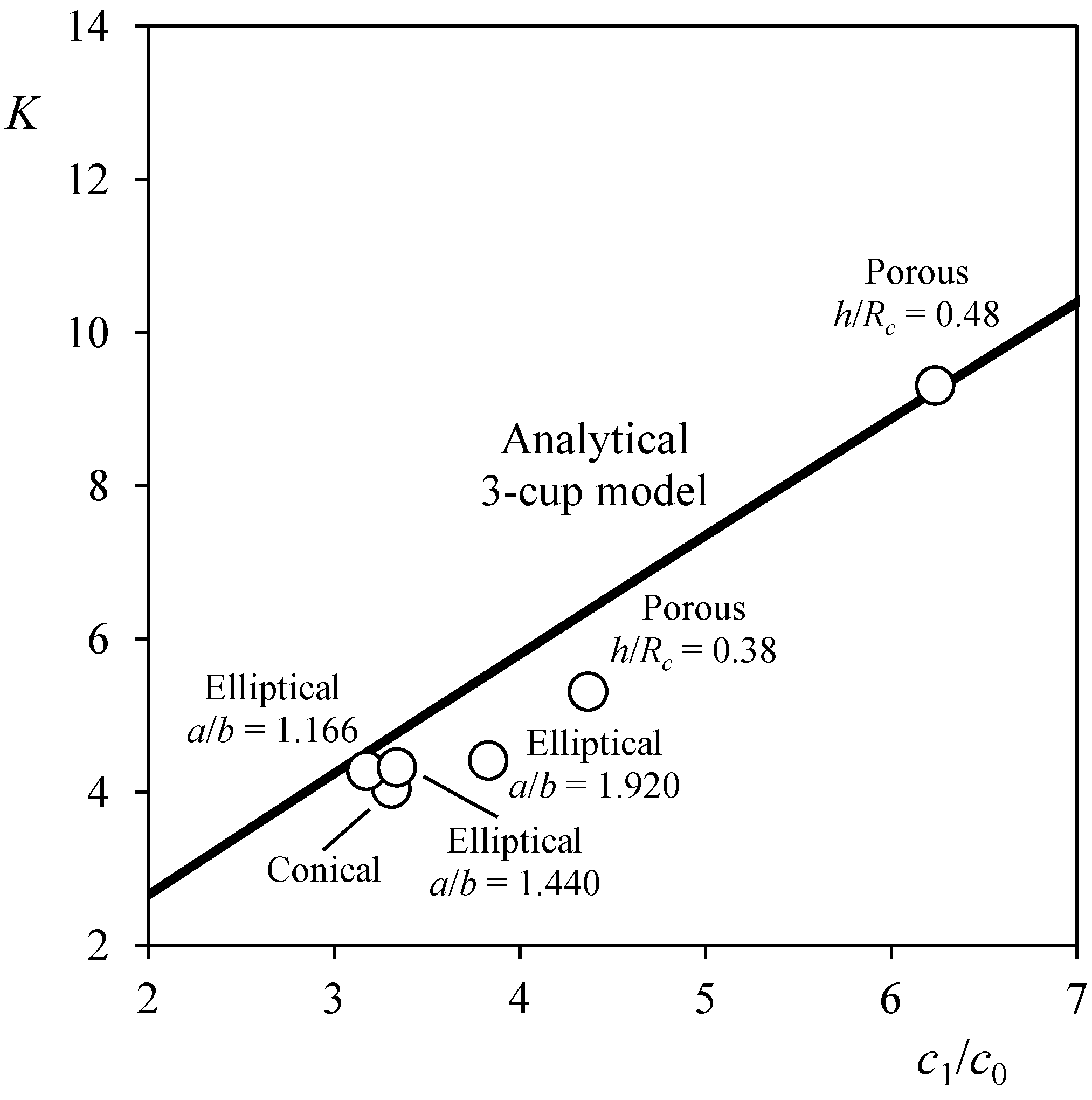
• The slope of the calibration curve, A_r, seemed (in that work) to have a direct relationship with the cups’ center rotation radius, R_rc, (that is, with the anemometer’s rotor radius). This relationship was also proven with an analytical model of the cup anemometer performance.

This last conclusion was checked with further studies at the IDR/UPM Institute by Pindado et al. [24] and Sanz-Andres et al. [29]. In these works, the calibration constants were proven to be dependent on geometric parameters of cup anemometer rotors, the following equations being derived:

$${\mathrm{A}}_r=\frac{{\mathrm{dA}}_r}{\mathrm{d}{R}_{rc}}{R}_{rc}+{\mathrm{A}}_{r0}=\frac{{\mathrm{dA}}_r}{\mathrm{d}{R}_{rc}}{R}_{rc}-S_c\left(\mathsf{\zeta }+\mathsf{\eta }{S}_c^{-\mathsf{\xi }}\right),$$

(3)

$$\mathrm{B}=\frac{\mathrm{dB}}{\mathrm{d}{R}_{rc}}{R}_{rc}+{\mathrm{B}}_0=\left(\mathsf{\epsilon }+\mathsf{\varphi }{S}_c^{-\mathsf{\gamma }}\right)R_{rc}-\mathsf{\mu }{S}_c^{-\mathsf{\psi }},$$

(4)

where R_rc is the cups’ center rotation radius, S_c, stands for the cups front area, and R_c is the cups radius (see Figure 4). The other terms present in the above equations: ζ η, ξ, ε, φ, γ, μ, and ψ are parameters to be extracted from experimental data.

In the mentioned work by Pindado et al. [24], two anemometers (Climatronics 100075 and Ornytion 107A, see pictures in Figure 5), were calibrated several times equipped with different rotors (varying the size of the same conical-shape cups and their distance to the rotation axis, i.e., R_rc). One of the most relevant conclusions of this study was that the slope dA_r/dR_rc only depends on the cups shape and not on their size (see Figure 5). Furthermore, in the analysis carried out by Sanz-Andres et al. [29], another important fact was revealed. The aerodynamic force on the cups is not acting on their center and even more, the center of the cup is not the average location of the aerodynamic center during one turn of the rotor (this has a quite important effect on the analytical modeling of cup anemometer performances).

Additionally, both the effect of the climatic conditions during the calibration process and cup anemometer performance degradation after several months working on the field were analyzed in the works by Pindado et al. [23,25]. The results of these analyses were as follows:

• Calibration constants, A and B, are affected by changes in air density, which, on the other hand, is driven mostly by changes in air temperature;
• These changes have a quite relevant impact on Annual Energy Production (AEP) estimations, depending on the selected wind sensor. Deviations of AEP up to 18% and 8% at 4 m·s⁻¹, and 7 m·s⁻¹ wind speeds were calculated for 0.1 kg·m⁻³ air density variations and first class anemometers;
• The anemometers degrade in large storage periods;
• Even showing a quite high level of wear and tear, it is quite difficult to establish degradation patterns of anemometers working on the field.

The output signal of cup anemometers has been also thoroughly studied at IDR/UPM Institute [26,30,31,34]. In steady wind the multi-pulse signal can be translated into a periodic rotation speed that shows three accelerations (and three decelerations) per turn of the rotor (see Figure 6). Therefore, from the pulsed-signal, it is possible to decompose the rotation rate of the anemometer, ω, into a Fourier series within one rotation period (see Figure 6).

$$\begin{array}{c}\omega \left(t\right)={\omega }_0+{\omega }_1\sin \left({\omega }_{0}t+{\phi }_1\right)+{\omega }_2\sin \left(2{\omega }_{0}t+{\phi }_2\right)+{\omega }_3\sin \left(3{\omega }_{0}t+{\phi }_3\right)\dots =\hfill \\ {\omega }_0+{\displaystyle \sum _{i=1}^{\infty }{\omega }_i\sin \left(i{\omega }_{0}t+{\phi }_i\right)}\hfill \end{array},$$

(5)

where i is the number of the harmonic term, ω_i its magnitude, and φ_i its phase angle (or angular deviation).

In the above equation, two important facts should be taken into account. First of all, the most relevant harmonic terms are the ones which are multiples of three, since due to the shape of the rotor (equipped with three cups) it accelerates three times per turn. Besides, all the other terms are noise due to turbulence or the wake downstream the anemometer’s body interaction with the rotor, with the obvious exception of the constant term, ω₀, that gives the average rotation speed, and the first harmonic term, ω₁, which reflects the perturbations that are repeated periodically once per turn. See the previous works by IDR/UPM Institute researchers [26,30,31].

The analysis of this first harmonic term has revealed itself as a very promising way to monitor the anemometer working condition. A quite relevant percentage of anemometers that are removed from a wind power generator for a recalibration process are damaged [74]. In Figure 7, a damaged A100 LK cup anemometer is shown, together with its calibration curve. This curve is compared to the one obtained with the anemometer equipped with a non-damaged rotor. In the top-right graph included in Figure 7, it can be observed that only a slight difference in the calibration curve is obtained, although the economic impact of this tiny deviation on a wind power plant could be huge. On the other hand, the damage is perfectly revealed by the first harmonic term (shown in the bottom-right graph of the figure).

Furthermore, a damaged cup anemometer might remain in a static position, that is, not-rotating, under normal or strong winds if one of the cups is missing or severely damaged. This can be a quite relevant problem, as the anemometer could still generate a pulsed signal that might be translated by the data-logger into a wind speed. The pulsed signal is generated by a small rotor-oscillation movement produced by the wake of the anemometer’s neck interacting with the rotor. Even worse, this completely wrong signal depends linearly on the wind speed and could induce a wind power generator to work out of the maximum efficiency point in case this problem is not anticipated, as shown by Pindado et al. [32].

Finally, the harmonic distribution of the rotor movement in steady wind speed represents a signature that defines a cup anemometer. Analyzing large series of two commercial cup anemometers calibrated at IDR/UPM facility, different patterns of the first and third harmonic terms statistical distribution were observed [34] (see Figure 8). The analysis of these frequency histograms might be used for quality control processes related to cup anemometer industrial production, as the best quality processes ensure a lower level of deviation among performances of different units of the same model (that is, a larger deviation of the harmonic histograms indicates greater differences on the unit’s performances).

3. Modeling Cup Anemometer Performances

As far as the authors’ knowledge, the first analytical model developed to study cup anemometer performances was proposed by Chree by the end of the 19th century [75]. After that, Schrenk [76] developed the classic model that was initially used by the IDR/UPM staff to study the cup anemometer behavior [22,29]. Since 2012, a new analytical model that takes into account the aerodynamic forces on the three cups of the rotor has been developed at IDR/UPM Institute [24,27,31,33]. At this point, it might be necessary to underline the importance of the analytical models. These models reproduce the behavior of complex processes (related to mechanics, thermodynamics, fluid mechanics, etc.), with quite simple equations that preserve the physics of the problem. In the present case, the goal is to analyze the performance of a rotor based on the cups’ aerodynamics.

The aforementioned model, developed in our previous works, is derived from the equation that defines the performance, that is, the rotation rate, ω, of a cup anemometer.

$$I\frac{\mathrm{d}\omega }{\mathrm{d}t}=Q_A+Q_f,$$

(6)

where I is the moment of inertia of the rotor, Q_A is the aerodynamic torque, and Q_f is the frictional torque that depends on the air temperature and the rotation rate [31]. The frictional torque is normally neglected, as its effect is only important at very low wind speeds (out of the calibration range). If the three cups of the rotor are taken into account the previous equation can be rewritten as follows:

$$\begin{array}{l}I\frac{\mathrm{d}\omega }{\mathrm{d}t}=\frac{1}{2}\rho S_c{R}_{rc}{V}_r^2\left(\theta \right)c_N\left(\alpha \left(\theta \right)\right)+\frac{1}{2}\rho S_c{R}_{rc}{V}_r^2\left(\theta +{120}^{\circ }\right)c_N\left(\alpha \left(\theta +{120}^{\circ }\right)\right)+\\ +\frac{1}{2}\rho S_c{R}_{rc}{V}_r^2\left(\theta +{240}^{\circ }\right)c_N\left(\alpha \left(\theta +{240}^{\circ }\right)\right)\end{array},$$

(7)

where V_r is the wind speed relative to the cups, c_N is the aerodynamic normal force coefficient, α is the wind direction with respect to the cups, and θ is the angle of the rotor with respect to a reference line (see sketch in Figure 9). The relative-to-the-cup wind speed can be expressed as:

$$V_r\left(\theta \right)=\sqrt{V^2+{\left(\omega R_{rc}\right)}^2-2V\omega R_{rc}\cos \left(\theta \right)}.$$

(8)

On the other hand, it is possible to derive an equation that correlates both the wind direction angle, α, and the position angle θ.

$$\tan \left(\alpha \right)=\frac{K\sin \left(\theta \right)}{K\cos \left(\theta \right)-1}.$$

(9)

In the above equation, the constant K is called the anemometer factor and it represents the ratio between the wind speed and the speed of the center of the cups.

$$K=\frac{V}{\omega R_{rc}}=\frac{{\mathrm{A}}_r{f}_r+\mathrm{B}}{2\pi f_r{R}_{rc}}=\frac{{\mathrm{A}}_r}{2\pi R_{rc}}\frac{1}{1-\left(\frac{\mathrm{B}}{V}\right)}.$$

(10)

Taking into account that the offset B is below 0.6 m·s⁻¹ for most commercial anemometers in the wind energy sector [22], it can be assumed that

$$K=\frac{{\mathrm{A}}_r}{2\pi R_{rc}}.$$

(11)

The aerodynamic force coefficient related to the cups, c_N, can be obtained, in a first approximation, from static measurements (that is, with no rotation of the cup) in wind tunnel [77]. However, this approach does not take into account the aerodynamic effect produced by the rotating flow over the cup. The aerodynamic force coefficient, c_N, can be expressed in terms of Fourier series, as it is a periodic function. See in Figure 9 the 1-harmonic and 6-harmonic terms Fourier series compared to the coefficient related to a conical cup experimentally measured. If the 1-harmonic equation is considered,

$$c_N\left(\alpha \right)=c_0+c_1\cos \left(\alpha \right).$$

(12)

Besides, the relationship between α and θ angles, previously defined by Equation (9), can be approximated as follows:

$$\cos \left(\alpha \right)={\eta }_0+{\eta }_1\cos \left(\theta \right)+{\eta }_2\cos {\left(\theta \right)}^2+{\eta }_3\cos {\left(\theta \right)}^3\dots$$

(13)

where:

$${\eta }_0=\frac{-1}{\sqrt{1+K^2}};{\eta }_1=\frac{K}{\sqrt{1+K^2}}-\frac{1}{K^2-1};{\eta }_2=\frac{1}{\sqrt{1+K^2}};{\eta }_3=\frac{K^2}{K^2-1}-\frac{K}{\sqrt{1+K^2}}.$$

(14)

Taking into account the above equations, the following expression can be derived from (7) in order to relate the anemometer factor, K, to the aerodynamic coefficients of the rotor cups:

$$0=\left(1+\frac{1}{K^2}\right)\left(1-\frac{1}{2}\frac{c_1}{c_0}\frac{1}{\sqrt{1+K^2}}\right)-\frac{1}{4}\frac{c_1}{c_0}\frac{1}{K}\left(\frac{K}{\sqrt{1+K^2}}+\frac{3K^2-4}{K^2-1}\right).$$

(15)

In Figure 10 the anemometer factor of several cases that were measured in wind tunnel (one anemometer, Climatronics 100075, equipped with different rotors in which the characteristics of the cups have been varied) are compared to the above equation. Results from of Equation (15) seem to reflect the tendencies shown by the testing results, with 13% average error [27].

However, this model presents a drawback, as it gives a single value of K without taking into account the geometric characteristics of the rotor (that affects the anemometer performance, as shown by Equations (3) and (4)). This was already observed in previous research campaigns at IDR/UPM, in which the effect of the ratio of the cups’ radius, R_c, to the cups’ center rotation radius, R_rc, defined as:

$$r_r=\frac{R_c}{R_{rc}},$$

(16)

was observed. In order to improve the model two effects were considered after an analysis campaign carried out by using Computer Fluid Dynamics (CFD) [78]. First of all, a phase angle δ was considered in relation to the aerodynamic force coefficient.

$$\begin{array}{l}{c}_N\left(\alpha \right)=c_0+c_1\cos \left(\alpha +\delta \right)=c_0+c_1\cos \left(\delta \right)\cos \left(\alpha \right)-c_1\sin \left(\delta \right)\sin \left(\alpha \right)=\\ c_0+c_{11}\cos \left(\alpha \right)-c_{12}\sin \left(\alpha \right)\end{array}.$$

(17)

Additionally, the aerodynamic force on the cup was not considered to be applied on the cups center, a deviation from the center (see sketch in Figure 11) being introduced in the model instead. This deviation d was also considered to be displaced a phase angle γ with respect to the cup position angle α in relation to the wind.

$$\begin{array}{l}\frac{d\left(\alpha \right)}{R_c}=e\sin \left(\alpha +\gamma \right)=e\cos \left(\gamma \right)\sin \left(\alpha \right)+e\sin \left(\gamma \right)\cos \left(\alpha \right)=\\ e_{11}\sin \left(\alpha \right)+e_{12}\cos \left(\alpha \right)\end{array}.$$

(18)

This approach takes into account the aerodynamic forces produced by cup rotation, together with the aforementioned forces derived from the cup direction with respect to the wind (that is, the aforementioned aerodynamic forces measured in static position). Making reasonable assumptions, this model was compared to testing results [33]. As it can be observed in Figure 11, the model was able to predict cup anemometer performances quite accurately, taking into account the effect of the geometric variable r_r. Furthermore, it is also fair to mention that the model seems to be less accurate for r_r > 0.45, that is, for rotors in which the cups are closer to the rotation axis (in relation to the cups size). In these cases, the rotation produces higher variations on the local wind speed around the cups, and probably causes this deviation.

Going back to the cup anemometer’s signal in steady wind and bearing in mind the work carried out in [31], it should be also pointed out that its Fourier series decomposition (Equation (5)) can be introduced in the general equation of the cup anemometer (Equation (7)), generating an interesting equation that takes into account the third harmonic term.

$$\begin{array}{l}\frac{I}{\frac{3}{2}\rho S_c{R}_{rc}{V}^2}\frac{\mathrm{d}\omega }{\mathrm{d}t}=-\frac{I3{\omega }_0{\omega }_3}{\frac{3}{2}\rho S_c{R}_{rc}{V}^2}\sin \left(3{\omega }_{0}t+{\phi }_3\right)\\ =\left(\left(1+\frac{1}{K^2}\right)(c_0+c_1({\eta }_0+\frac{1}{2}{\eta }_2))-\frac{1}{K}{c}_1({\eta }_1+\frac{3}{4}{\eta }_3)\right)\\ +\left(\left(1+\frac{1}{K^2}\right){\eta }_3-\frac{2}{K}{\eta }_2\right)\frac{c_1}{4}\cos \left(3\theta \right)\end{array}.$$

(19)

As it is obvious, the second term at the right side of the above equation is indeed the Equation (15), which gives the average rotation speed of the cup anemometer as a function of the ratio c₁/c₀. Additionally, the remaining terms give information on the third harmonic term of the rotation rate. The following equation can then be derived:

$$\begin{array}{l}\frac{{\omega }_3}{{\omega }_0}=\left(\frac{\pi }{8}\right)\left(\frac{\rho R_{rc}^5}{I}\right)\left|\left(\left(K^2+1\right){\eta }_3-2K{\eta }_2\right)\right|c_1{r}_r^2\\ \approx \left(\frac{\pi }{8}\right)\left(\frac{\rho R_{rc}^5}{I}\right)\left(0.5308{\left(\frac{c_1}{c_0}-1\right)}^{-1.599}-0.5\right)c_1{r}_r^2\end{array}$$

(20)

This is an important result that suggests the existence of a theoretical minimum for this third harmonic term for c₁/c₀ ≈ 2.05.

Finally, the importance of modeling cup anemometer performances should be emphasized in order to produce new improvements and designs that could increase the accuracy of the wind speed measurements. In this sense, it is worth mentioning the work by Dahlberg et al. [79] that produced in 2001 a new rotor design (Patent No.: US 2004/0083806 A1 [80], see Figure 12), or the one from Thies Clima (Patent No.: EP 1489427 B1 [81]), or the more recent development by Hong in 2012 [82] (Patent No.: US 2012/0266692 A1, see Figure 12).

4. Conclusions

In the present work, the research on cup anemometer performances carried out at IDR/UPM has been summarized. This research has been focused on the following two aspects, although both are related:

• The analysis of the performance based on experimental results as follows:

  ○

  Force on isolated cups;

  ○

  Calibrations performed on both commercial anemometers and anemometers equipped with special-design rotors;

  ○

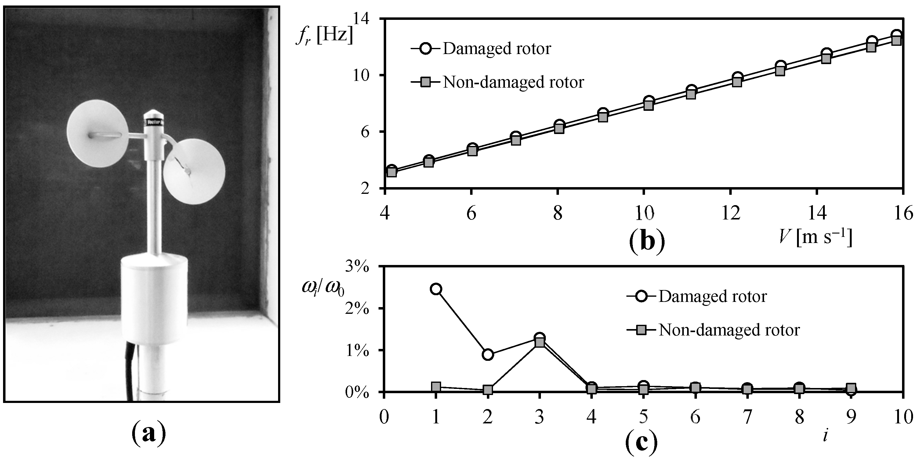
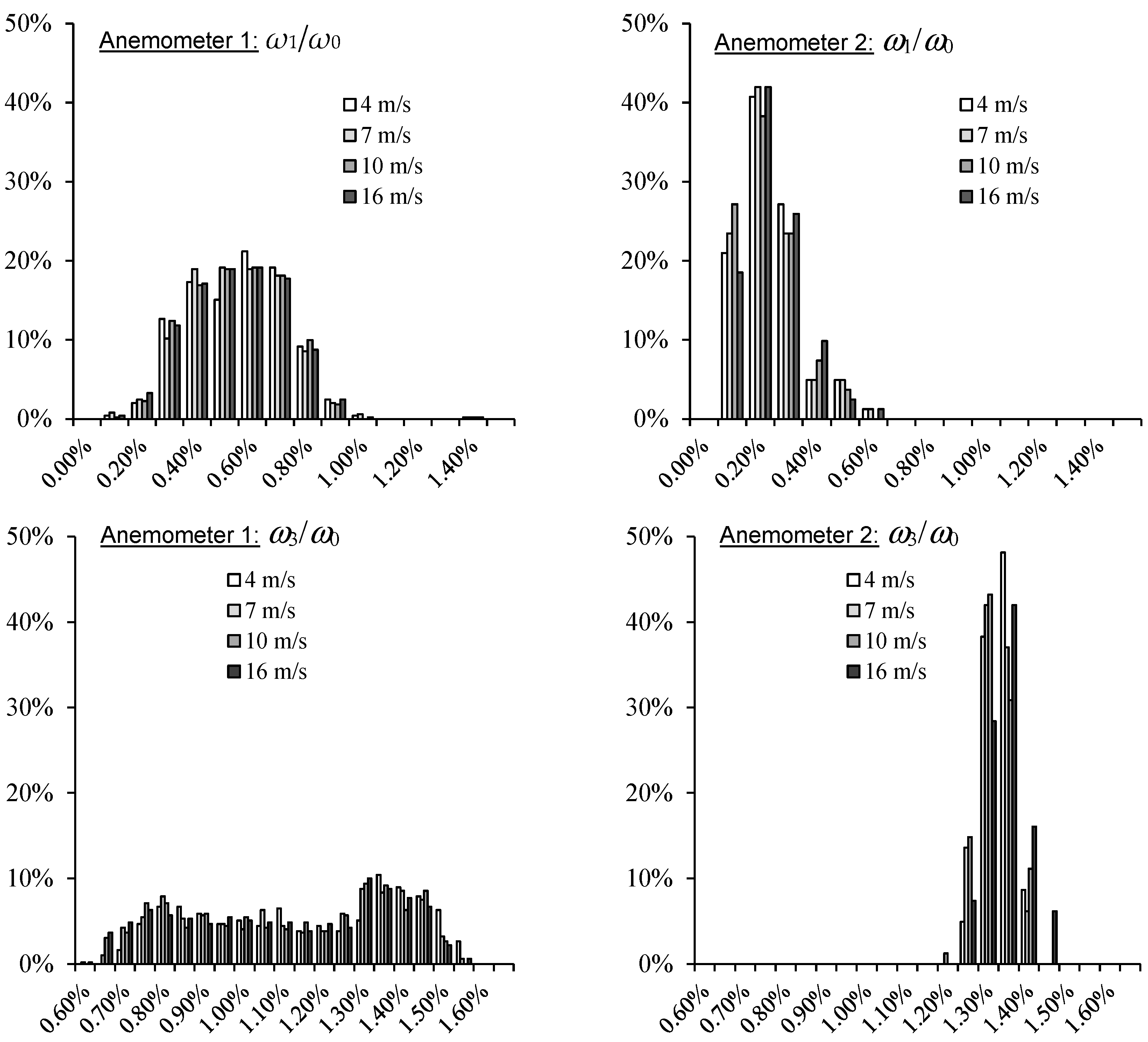
  The output signal of the cup anemometers.

• The analytical study of the cup anemometer performances with a new methodology developed consequently. All expertise gained with the analysis of testing results was a fundamental basis for this analytical work. It should be underlined the importance of analytical models in order to produce better sensors in the future, as by using these models, a reduction of costs (measured in time and calculation resources) can be achieved in the first stages of the designing process.

For future works, some of them being in progress at the IDR/UPM Institute, it could be interesting to analyze the performances of working-on-the-field cup anemometers, taking into account the evolution of the rotation rate harmonic terms after long service periods of the wind sensor. Besides, it should be also of great interest to understand the aerodynamic forces and pressure distribution on rotating cups by means of experimental testing and CFD analysis.

References

1. Sanz-Andrés, A.; Meseguer, J. El satélite español UPM-Sat 1. Mundo Científico 1996, 169, 560–567. [Google Scholar]
2. Meseguer, J.; Sanz, A.; Lopez, J. Liquid bridge breakages aboard spacelab-D1. J. Cryst. Growth 1986, 78, 325–334. [Google Scholar] [CrossRef]
3. Sanz-Andrés, A.; Meseguer, J.; Perales, J.M.; Santiago-Prowald, J. A small platform for astrophysical research based on the UPM-Sat 1 satellite of the Universidad Politécnica de Madrid. Adv. Space Res. 2003, 31, 375–380. [Google Scholar] [CrossRef] [Green Version]
4. Sanz-Andrés, A.; Rodríguez-De-Francisco, P.; Santiago-Prowald, J. The Experiment CPLM (Comportamiento De Puentes Líquidos En Microgravedad) on Board MINISAT 01. In Science with Minisat 01; Springer: Dordrecht, The Netherlands, 2001; pp. 97–121. [Google Scholar]
5. Neefs, E.; Vandaele, A.C.; Drummond, R.; Thomas, I.R.; Berkenbosch, S.; Clairquin, R.; Delanoye, S.; Ristic, B.; Maes, J.; Bonnewijn, S.; et al. NOMAD spectrometer on the ExoMars trace gas orbiter mission: Part 1—Design, manufacturing and testing of the infrared channels. Appl. Opt. 2015, 54, 8494–8520. [Google Scholar] [CrossRef] [PubMed]
6. Fernández Rico, G.; Perez-Grande, I. Diseño térmico preliminar del Instrumento PHI de Solar Orbiter. In Actas del VII Congreso Nacional de Ingeniería Termodinámica—CNIT7; Universidad del País Vasco: Bilbao, España, 2011. [Google Scholar]
7. Patel, M.R.; Antoine, P.; Mason, J.; Leese, M.; Hathi, B.; Stevens, A.H.; Dawson, D.; Gow, J.; Ringrose, T.; Holmes, J.; et al. NOMAD spectrometer on the ExoMars trace gas orbiter mission: Part 2—Design, manufacturing, and testing of the ultraviolet and visible channel. Appl. Opt. 2017, 56, 2771–2782. [Google Scholar] [CrossRef] [PubMed]
8. Abdellaoui, G.; Abe, S.; Acheli, A.; Adams, J.H.; Ahmad, S.; Ahriche, A.; Albert, J.N.; Allard, D.; Alonso, G.; Anchordoqui, L.; et al. Meteor studies in the framework of the JEM-EUSO program. Planet. Space Sci. 2017, 143, 245–255. [Google Scholar] [CrossRef]
9. Abdellaoui, G.; Abe, S.; Acheli, A.; Adams, J.H.; Ahmad, S.; Ahriche, A.; Albert, J.-N.; Allard, D.; Alonso, G.; Anchordoqui, L.; et al. Cosmic ray oriented performance studies for the JEM-EUSO first level trigger. Nucl. Instrum. Methods Phys. Res. Sect. A Accel. Spectrom. Detect. Assoc. Equip. 2017, 866, 150–163. [Google Scholar] [CrossRef]
10. Cubas, J.; Farrahi, A.; Pindado, S. Magnetic Attitude Control for Satellites in Polar or Sun-Synchronous Orbits. J. Guid. Control Dyn. 2015, 38, 1947–1958. [Google Scholar] [CrossRef]
11. Roibás-Millán, E.; Alonso-Moragón, A.; Jiménez-Mateos, A.; Pindado, S. On solar panels testing for small-size satellites. The UPMSAT-2 mission. Meas. Sci. Technol. 2017. [Google Scholar] [CrossRef]
12. Pindado, S.; Meseguer, J. Wind tunnel study on the influence of different parapets on the roof pressure distribution of low-rise buildings. J. Wind Eng. Ind. Aerodyn. 2003, 91, 1133–1139. [Google Scholar] [CrossRef]
13. Franchini, S.; Pindado, S.; Meseguer, J.; Sanz-Andrés, A. A parametric, experimental analysis of conical vortices on curved roofs of low-rise buildings. J. Wind Eng. Ind. Aerodyn. 2005, 93, 639–650. [Google Scholar] [CrossRef]
14. Pindado, S.; Meseguer, J.; Franchini, S. The influence of the section shape of box-girder decks on the steady aerodynamic yawing moment of double cantilever bridges under construction. J. Wind Eng. Ind. Aerodyn. 2005, 93, 547–555. [Google Scholar] [CrossRef]
15. Pindado, S.; Meseguer, J.; Franchini, S. Influence of an upstream building on the wind-induced mean suction on the flat roof of a low-rise building. J. Wind Eng. Ind. Aerodyn. 2011, 99, 889–893. [Google Scholar] [CrossRef] [Green Version]
16. Sanz-Andrés, A.; Santiago-Prowald, J. Train-induced pressure on pedestrians. J. Wind Eng. Ind. Aerodyn. 2002, 90, 1007–1015. [Google Scholar] [CrossRef]
17. Sanz-Andrés, A.; Santiago-Prowald, J.; Baker, C.; Quinn, A. Vehicle-induced loads on traffic sign panels. J. Wind Eng. Ind. Aerodyn. 2003, 91, 925–942. [Google Scholar] [CrossRef] [Green Version]
18. Pindado, S.; Sanz, A.; Sebastian, F.; Perez-grande, I.; Alonso, G.; Perez-Alvarez, J.; Sorribes-Palmer, F.; Cubas, J.; Garcia, A.; Roibas, E.; Fernandez, A. Master in Space Systems, an Advanced Master’s Degree in Space Engineering. In ATINER’S Conference Paper Series, No: ENGEDU2016-1953; Athens Institute for Education and Research: Athens, Greece, 2016; pp. 1–16. [Google Scholar]
19. Pindado Carrion, S.; Roibás-Millán, E.; Cubas Cano, J.; García, A.; Sanz Andres, A.P.; Franchini, S.; Pérez Grande, M.I.; Alonso, G.; Pérez-Álvarez, J.; Sorribes-Palmer, F.; et al. The UPMSat-2 Satellite: An academic project within aerospace engineering education. In ATINER’S Conference Paper Series. Working Paper; Athens Institute for Education and Research: Athens, Greece, 2017. [Google Scholar]
20. Pindado, S.; Roibas, E.; Cubas, J.; Sorribes-Palmer, F.; Sanz-Andrés, A.; Franchini, S.; Perez-Grande, I.; Zamorano, J.; De La Puente, J.A.; Perez-Alvarez, J.; et al. MUSE. Master in Space Systems at Universidad Politécnica de Madrid (UPM). Available online: https://www.researchgate.net/project/MUSE-Master-in-Space-Systems-at-Universidad-Politecnica-de-Madrid-UPM (accessed on 12 November 2017).
21. Cubas, J.; Sorribes-Palmer, F.; Pindado, S. The use of STK as educational tool in the MUSE (Master in Space Systems), an Advanced Master’s Degree in Space. In Proceedings of the AGI’s 2nd International Users Conference: Ciao Roma, Roma, Italy, 6–18 November 2016. [Google Scholar]
22. Pindado, S.; Vega, E.; Martínez, A.; Meseguer, E.; Franchini, S.; Pérez, I. Analysis of calibration results from cup and propeller anemometers. Influence on wind turbine Annual Energy Production (AEP) calculations. Wind Energy 2011, 14, 119–132. [Google Scholar] [CrossRef]
23. Pindado, S.; Barrero-Gil, A.; Sanz, A. Cup Anemometers’ Loss of Performance Due to Ageing Processes, and Its Effect on Annual Energy Production (AEP) Estimates. Energies 2012, 5, 1664–1685. [Google Scholar] [CrossRef] [Green Version]
24. Pindado, S.; Pérez, J.; Avila-Sanchez, S. On cup anemometer rotor aerodynamics. Sensors 2012, 12, 6198–6217. [Google Scholar] [CrossRef] [PubMed] [Green Version]
25. Pindado, S.; Sanz, A.; Wery, A. Deviation of Cup and Propeller Anemometer Calibration Results with Air Density. Energies 2012, 5, 683–701. [Google Scholar] [CrossRef]
26. Pindado, S.; Cubas, J.; Sanz-Andrés, A. Aerodynamic analysis of cup anemometers performance. The stationary harmonic response. Sci. World J. 2013, 2013, 197325. [Google Scholar] [CrossRef] [PubMed]
27. Pindado, S.; Pérez, I.; Aguado, M. Fourier analysis of the aerodynamic behavior of cup anemometers. Meas. Sci. Technol. 2013, 24, 065802. [Google Scholar] [CrossRef]
28. Pindado, S.; Cubas, J.; Sorribes-Palmer, F. The Cup Anemometer, a Fundamental Meteorological Instrument for the Wind Energy Industry. Research at the IDR/UPM Institute. Sensors 2014, 14, 21418–21452. [Google Scholar] [CrossRef] [PubMed]
29. Sanz-Andrés, A.; Pindado, S.; Sorribes, F. Mathematical analysis of the effect of the rotor geometry on cup anemometer response. Sci. World J. 2014, 2014, 537813. [Google Scholar] [CrossRef] [PubMed]
30. Vega, E.; Pindado, S.; Martínez, A.; Meseguer, E.; García, L. Anomaly detection on cup anemometers. Meas. Sci. Technol. 2014, 25, 127002. [Google Scholar] [CrossRef]
31. Pindado, S.; Cubas, J.; Sorribes-Palmer, F. On the harmonic analysis of cup anemometer rotation speed: A principle to monitor performance and maintenance status of rotating meteorological sensors. Measurement 2015, 73, 401–418. [Google Scholar] [CrossRef]
32. Pindado, S.; Cubas, J.; Sorribes-Palmer, F. On the Analytical Approach to Present Engineering Problems: Photovoltaic Systems Behavior, Wind Speed Sensors Performance, and High-Speed Train Pressure Wave Effects in Tunnels. Math. Probl. Eng. 2015, 2015, 897357. [Google Scholar] [CrossRef]
33. Pindado, S.; Ramos-Cenzano, A.; Cubas, J. Improved analytical method to study the cup anemometer performance. Meas. Sci. Technol. 2015, 26, 1–6. [Google Scholar] [CrossRef]
34. Martínez, A.; Vega, E.; Pindado, S.; Meseguer, E.; García, L. Deviations of cup anemometer rotational speed measurements due to steady state harmonic accelerations of the rotor. Measurement 2016, 90, 483–490. [Google Scholar] [CrossRef] [Green Version]
35. Cuerva, A.; Sanz-Andrés, A. On sonic anemometer measurement theory. J. Wind Eng. Ind. Aerodyn. 2000, 88, 25–55. [Google Scholar] [CrossRef]
36. Cuerva, A.; Sanz-Andrés, A.; Navarro, J. On multiple-path sonic anemometer measurement theory. Exp. Fluids 2003, 34, 345–357. [Google Scholar] [CrossRef]
37. Cuerva, A.; Sanz-Andrés, A.; Lorenz, R.D. Sonic anemometry of planetary atmospheres. J. Geophys. Res. Planets 2003, 108, 1–7. [Google Scholar] [CrossRef]
38. Franchini, S.; Sanz-Andrés, A.; Cuerva, A. Measurement of velocity in rotational flows using ultrasonic anemometry: The flowmeter. Exp. Fluids 2007, 42, 903–911. [Google Scholar] [CrossRef]
39. Franchini, S.; Sanz-Andrés, A.; Cuerva, A. Effect of the pulse trajectory on ultrasonic fluid velocity measurement. Exp. Fluids 2007, 43, 969–978. [Google Scholar] [CrossRef]
40. Wagner, R.; Courtney, M.; Gottschall, J.; Lindelöw-Marsden, P. Accounting for the speed shear in wind turbine power performance measurement. Wind Energy 2011, 14, 993–1004. [Google Scholar] [CrossRef]
41. Lang, S.; McKeogh, E. LIDAR and SODAR measurements of wind speed and direction in upland terrain for wind energy purposes. Remote Sens. 2011, 3, 1871–1901. [Google Scholar] [CrossRef]
42. Bradley, S. Aspects of the Correlation between Sodar and Mast Instrument Winds. J. Atmos. Ocean. Technol. 2013, 30, 2241–2247. [Google Scholar] [CrossRef]
43. Sanz Rodrigo, J.; Borbón Guillén, F.; Gómez Arranz, P.; Courtney, M.S.; Wagner, R.; Dupont, E. Multi-site testing and evaluation of remote sensing instruments for wind energy applications. Renew. Energy 2013, 53, 200–210. [Google Scholar] [CrossRef]
44. Hasager, C.; Stein, D.; Courtney, M.; Peña, A.; Mikkelsen, T.; Stickland, M.; Oldroyd, A. Hub Height Ocean Winds over the North Sea Observed by the NORSEWInD Lidar Array: Measuring Techniques, Quality Control and Data Management. Remote Sens. 2013, 5, 4280–4303. [Google Scholar] [CrossRef] [Green Version]
45. Hobby, M.; Gascoyne, M.; Marsham, J.H.; Bart, M.; Allen, C.; Engelstaedter, S.; Fadel, D.M.; Gandega, A.; Lane, R.; McQuaid, J.B.; et al. The Fennec Automatic Weather Station (AWS) Network: Monitoring the Saharan Climate System. J. Atmos. Ocean. Technol. 2013, 30, 709–724. [Google Scholar] [CrossRef]
46. Mikkelsen, T. Lidar-based Research and Innovation at DTU Wind Energy—A Review. J. Phys. Conf. Ser. 2014, 524, 12007. [Google Scholar] [CrossRef]
47. Serrano González, J.; Burgos Payán, M.; Santos, J.M.R.; González-Longatt, F. A review and recent developments in the optimal wind-turbine micro-siting problem. Renew. Sustain. Energy Rev. 2014, 30, 133–144. [Google Scholar] [CrossRef]
48. Bradley, S.; Strehz, A.; Emeis, S. Remote sensing winds in complex terrain—A review. Meteorol. Z. 2015, 24, 547–555. [Google Scholar] [CrossRef]
49. Kim, D.; Kim, T.; Oh, G.; Huh, J.; Ko, K. A comparison of ground-based LiDAR and met mast wind measurements for wind resource assessment over various terrain conditions. J. Wind Eng. Ind. Aerodyn. 2016, 158, 109–121. [Google Scholar] [CrossRef]
50. Kang, D.; Hyeon, J.; Yang, K.; Huh, J.; Ko, K. Analysis and Verification of Wind Data from Ground-based LiDAR. Int. J. Renew. Energy Res. 2017, 7, 937–945. [Google Scholar]
51. Cheynet, E.; Jakobsen, J.B.; Snæbjörnsson, J.; Reuder, J.; Kumer, V.; Svardal, B. Assessing the potential of a commercial pulsed lidar for wind characterisation at a bridge site. J. Wind Eng. Ind. Aerodyn. 2017, 161, 17–26. [Google Scholar] [CrossRef]
52. Li, J.; Yu, X. (Bill) LiDAR technology for wind energy potential assessment: Demonstration and validation at a site around Lake Erie. Energy Convers. Manag. 2017, 144, 252–261. [Google Scholar] [CrossRef]
53. Khan, K.S.; Tariq, M. Wind resource assessment using SODAR and meteorological mast—A case study of Pakistan. Renew. Sustain. Energy Rev. 2017. [Google Scholar] [CrossRef]
54. Dubov, D.; Aprahamian, B.; Aprahamian, M. Comparison between Conventional Wind Measurement Systems and SODAR Systems for Remote Sensing Including Examination of Real Wind Data. In Proceedings of the 2017 15th International Conference on Electrical Machines, Drives and Power Systems (ELMA), Sofia, Bulgaria, 1–3 June 2017; pp. 106–109. [Google Scholar]
55. Pedersen, B.M.; Hansen, K.S.; Øye, S.; Brinch, M.; Fabian, O. Some experimental investigations on the influence of the mounting arrangements on the accuracy of cup-anemometer measurements. J. Wind Eng. Ind. Aerodyn. 1992, 39, 373–383. [Google Scholar] [CrossRef]
56. Pedersen, T.F.; Sørensen, N.N.; Madsen, H.A.; Courtney, M.; Møller, R.; Enevoldsen, P.; Egedal, P. Spinner anemometry—An innovative wind measurement concept. In Proceedings of the 2007 European Wind Energy Conference and Exhibition (EWEC 2007), Milan, Italy, 7–10 May 2007. [Google Scholar]
57. Wagner, R.; Pedersen, T.F.; Courtney, M.; Antoniou, I.; Davoust, S.; Rivera, R.L. Power curve measurement with a nacelle mounted lidar. Wind Energy 2014, 17, 1441–1453. [Google Scholar] [CrossRef]
58. Pedersen, T.F.; Demurtas, G.; Zahle, F. Calibration of a spinner anemometer for yaw misalignment measurements. Wind Energy 2015, 18, 1933–1952. [Google Scholar] [CrossRef] [Green Version]
59. Demurtas, G.; Pedersen, T.F.; Zahle, F. Calibration of a spinner anemometer for wind speed measurements. Wind Energy 2016, 19, 2003–2021. [Google Scholar] [CrossRef]
60. Robinson, T.R. On a New Anemometer. Proc. R. Ir. Acad. 1847, 4, 566–572. [Google Scholar]
61. Robinson, T.R. On the Determination of the Constants of the Cup Anemometer by Experiments with a Whirling Machine. Philos. Trans. R. Soc. Lond. 1878, 169, 777–822. [Google Scholar] [CrossRef]
62. Robinson, T.R. On the Constants of the Cup Anemometer. Proc. R. Soc. Lond. 1880, 30, 572–574. [Google Scholar] [CrossRef]
63. Robinson, T.R. On the Determination of the Constants of the Cup Anemometer by Experiments with a Whirling Machine. Part II. Philos. Trans. R. Soc. Lond. 1880, 171, 1055–1070. [Google Scholar] [CrossRef]
64. Brazier, M.C.-E. Sur la variation des indications des anémomètres Robinson et Richard en fonction de l’inclinaison du vent. C. R. Séances Acad. Sci. 1920, 170, 610–612. [Google Scholar]
65. Brazier, M.C.-E. Sur la comparabilité des anémomètres. C. R. Séances Acad. Sci. 1921, 172, 843–845. [Google Scholar]
66. Brazier, M.C.-E. On the Comparability of Anemometers. Mon. Weather Rev. 1921, 49, 575. [Google Scholar] [CrossRef]
67. Marvin, C.F. Recent Advances in Anemometry. Mon. Weather Rev. 1934, 62, 115–120. [Google Scholar] [CrossRef]
68. Patterson, J. The cup anemometer. Trans. R. Soc. Can. Ser. III 1926, 20, 1–54. [Google Scholar]
69. Spilhaus, A.F.; Rossby, C. Analysis of the Cup Anemometer (Meteorological Course. Professional Notes—No. 7); Massachusetts Institute of Technology: Cambridge, MA, USA, 1934. [Google Scholar]
70. Fergusson, S.P. Harvard Meteorological Studies No. 4. Experimental Studies of Cup Anemometers; Harvard University Press: Cambridge, MA, USA, 1939. [Google Scholar]
71. Sheppard, P.A. An improved design of cup anemometer. J. Sci. Instrum. 1940, 17, 218–221. [Google Scholar] [CrossRef]
72. MEASNET. Cup Anemometer Calibration Procedure, Version 1 (September 1997, Updated 24/11/2008); MEASNET: Madrid, Spain, 1997. [Google Scholar]
73. MEASNET. Cup Anemometer Calibration Procedure, Version 2 (October 2009); MEASNET: Madrid, Spain, 2009. [Google Scholar]
74. Stefanatos, N.; Papadopoulos, P.; Binopoulos, E.; Kostakos, A.; Spyridakis, G. Effects of long term operation on the performance characteristics of cup anemometers. In Proceedings of the European Wind Energy Conference and Exhibition (EWEC 2007), Milan, Italy, 7–10 May 2007; pp. 1–6. [Google Scholar]
75. Chree, C. Contribution to the Theory of the Robinson Cup-Anemometer. Lond. Edinb. Dublin Philos. Mag. J. Sci. 1895, 40, 63–90. [Google Scholar] [CrossRef]
76. Schrenk, O. Über die Trägheitsfehler des Schalenkreuz-Anemometers bei schwankender Windstärke. Z. Tech. Phys. 1929, 10, 57–66. [Google Scholar]
77. Brevoort, M.J.; Joyner, U.T. Experimental Investigation of the Robinson-Type Cup Anemometer; NACA TN-513; Government Printing Office: Washington, DC, USA, 1935.
78. Ramos Cenzano, A. Análisis Mediante Cálculo Numérico (CFD) del Comportamiento de Anemómetros de Cazoletas; Universidad Politécnica de Madrid: Madrid, Spain, 2014. [Google Scholar]
79. Dahlberg, J.-Å.; Gustavsson, J.; Ronsten, G.; Pedersen, T.F.; Paulsen, U.S.; Westermann, D. Development of a Standardised Cup Anemometer Suited to Wind Energy Applications—(Classcup); Contract JOR3-C T98-0263; Publishable Final Report; Aeronautical Research Institute of Sweden: Ulvsunda, Sweden, 2001; pp. 1–37. [Google Scholar]
80. Dahlberg, J.-A. Cup Anemometer. U.S. Patent 2004/0083806 A1, 6 May 2017. [Google Scholar]
81. Westermann, D. Selektives Messen einer Richtungskomponente der Strömungsgeschwindigkeit mit einem Schalensternanemometer. EP 1489427 B1, 12 November 2008. [Google Scholar]
82. Hong, S.-H. Asymmetric-Cup Anemometer. U.S. Patent 2012/0266692 A1, 25 October 2012. [Google Scholar]
Figure 1. Old Robinson cup anemometer (a) and Thies Clima 4.3350 cup anemometer (b).
Energies 10 01860 g001
Figure 2. Installed wind power in some of the most relevant countries (a) and its annual growth (b). Source: Global Wind Energy Council.
Energies 10 01860 g002
Figure 3. Two different calibrations performed on the same Thies Clima 4.3350 cup anemometer (see Figure 1): AC calibration (13 measurement points taken within a wind speed bracket from 4 m·s−1 to 16 m·s−1) and AD calibration (nine measurement points taken within a wind speed bracket from 4 m·s−1 to 23 m·s−1). The transfer function related to the AC calibration has been included in the graph. The coefficient of determination related to this linear fitting, R2, is also included in the graph (AC calibrations require high values of this coefficient).
Energies 10 01860 g003
Figure 4. Sketch of a cup anemometer. The more important dimensions of the rotor, the cups’ center rotation radius, Rrc, and the cups radius, Rc, are indicated in the figure.
Energies 10 01860 g004
Figure 5. Climatronics 100075 with a Rc = 30 mm and Rrc = 100 mm rotor (a) and Ornytion 107A with a Rc = 30 mm and Rrc = 40 mm rotor (b) cup anemometers. Ar (c) and B (d) calibration coefficients (see Equation (2)), in relation to the cups’ center rotation radius, Rrc, for two different size conical cups (Rc = 25 mm and Rc = 80 mm).
Energies 10 01860 g005
Figure 6. Voltage output signal, uout, from a Climatronics 100075 cup anemometer (a). The rotation rate derived from that signal is included in the (b) graph, whereas the Fourier series extracted from the rotation rate is included in the (c) graph, where the harmonic terms, ωi/ω0, are compared (see also Equation (5)).
Energies 10 01860 g006
Figure 7. Damaged A100 LK cup anemometer after service period (a). Calibration curve of this anemometer compared to the one of that anemometer equipped with a non-damaged rotor (b). Fourier series decomposition of the aforementioned cup anemometer rotation rate along one turn of the rotor, see Equation (5) (c).
Energies 10 01860 g007
Figure 8. First and third harmonic terms, ω1/ω0 and ω3/ω0, histograms from large series of two first class cup anemometers calibrated at Instituto Universitario de Microgravedad “Ignacio Da Riva” (IDR/UPM): Anemometer-1 and Anemometer-2.
Energies 10 01860 g008
Figure 9. Normal aerodynamic force coefficient, cN, of the Brevoort & Joyner Type-II (conical) cups [77]. See in the sketch the variables involved in the rotation of an anemometer cup: normal aerodynamic force on the cup, N, wind speed, V, relative wind speed to the cup, Vr, rotor rotation angle, θ, rotor rotational speed, ω, and wind direction with respect to the cup, α. The 1-harmonic term Fourier series approximation (Equation (12)) to the Type-II cup has been plotted, together with the more accurate 6-harmonic terms Fourier series approximation.
Energies 10 01860 g009
Figure 10. Results of the developed analytical model (Equation (15)), compared to testing results. In the graph, the anemometer factors, K, measured and calculated from anemometers equipped with the same rotor varying only the aerodynamic characteristics of the cups, are plotted as a function of those aerodynamic characteristics c0/c1 (see Equation (12)).
Energies 10 01860 g010
Figure 11. (a) Sketch of the variables involved in the rotation movement of an anemometer’s cup. See that the normal aerodynamic force, N, is considered to be deviated from the center of the cup. (b) Anemometer factors, K, measured from anemometers equipped with different rotors (varying the cups’ radius, Rc, and the cups center rotation radius, Rrc), in relation to the geometric ratio rr = Rc/Rrc. In the graph, the results from the analytical model developed (Equation (15)) and its improved version (Equations (17) and (18)) are included.
Energies 10 01860 g011
Figure 12. Examples of cups anemometer rotor design. Design by Dahlberg (Patent No.: US 2004/0083806 A1) (a), and design by Hong (Patent No.: US 2012/0266692 A1) (b).
Energies 10 01860 g012