6.2. Evaluation of Classification Accuracy
We used a standard deep learning technique called
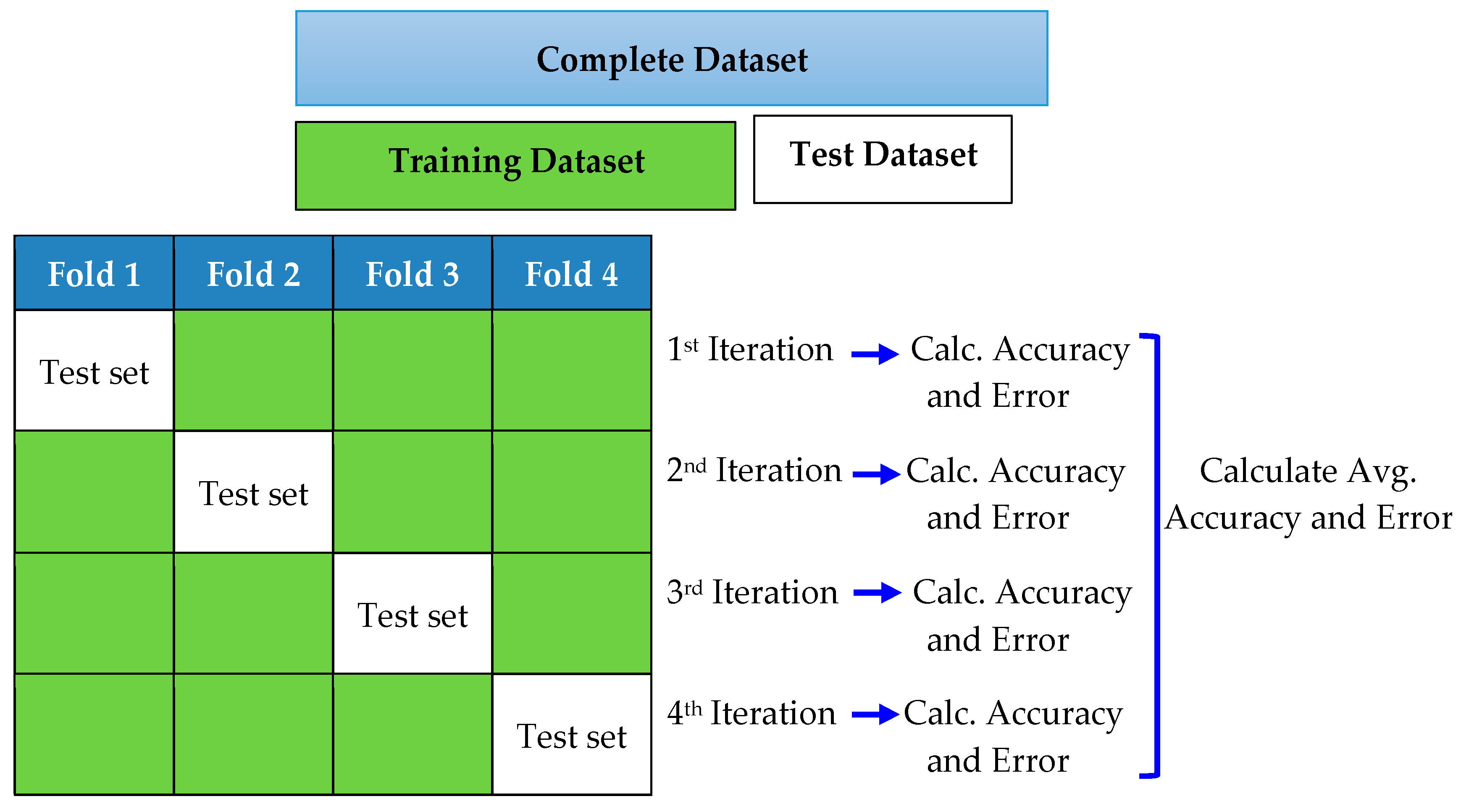
k-fold cross-validation to evaluate the classification accuracy and prediction error of the model. In fact,
k-fold cross-validation is a model validation method where data is divided into
K smaller sets and (
k − 1) part of which is used to train the model, and the rest of the part is used as validation data to test the model. This process is repeated on all
k subsets so that each subset is used as validation data exactly once, and as training data (
k − 1) times. Finally, we averaged the classification accuracy and error rates of the
k experiments to obtain a single performance metric. In
k-fold cross-validation,
k is typically 10, which is a suitable choice for most applications. To reduce the computational time, we used 4-fold cross-validation in this study, as shown in
Figure 8.
In
Figure 8, the complete dataset is divided into four subsets, and the model is trained and tested four times. In each iteration, one subset was used to test the model arising from training the classifier on the other three subsets. We assessed the average performance of the model by calculating the estimated error for each subset.
6.4. Confusion Matrix
To visualize the performance of proposed method, we used a classification matrix known as “confusion matrix”. A confusion matrix summarizes the classification performance and provides a visual representation of actual versus predicted class accuracies. In the confusion matrix, each column represents the predicted class whereas each row represents the actual class respectively. A simple structure of confusion matrix having three class is shown in
Table 6.
Furthermore, a confusion matrix is a table that reports the counts of true positives, false positives, true negatives and false negatives which are defined as:
True Positive (TP). The label belongs to the class, and it is correctly predicted.
False Positive (FP). The label does not belong to the class, but classifier predicted as positive.
True Negative (TN). The label does not belong to the class, and it is correctly predicted.
False Negative (FN). The label does belong to the class but is predicted as negative.
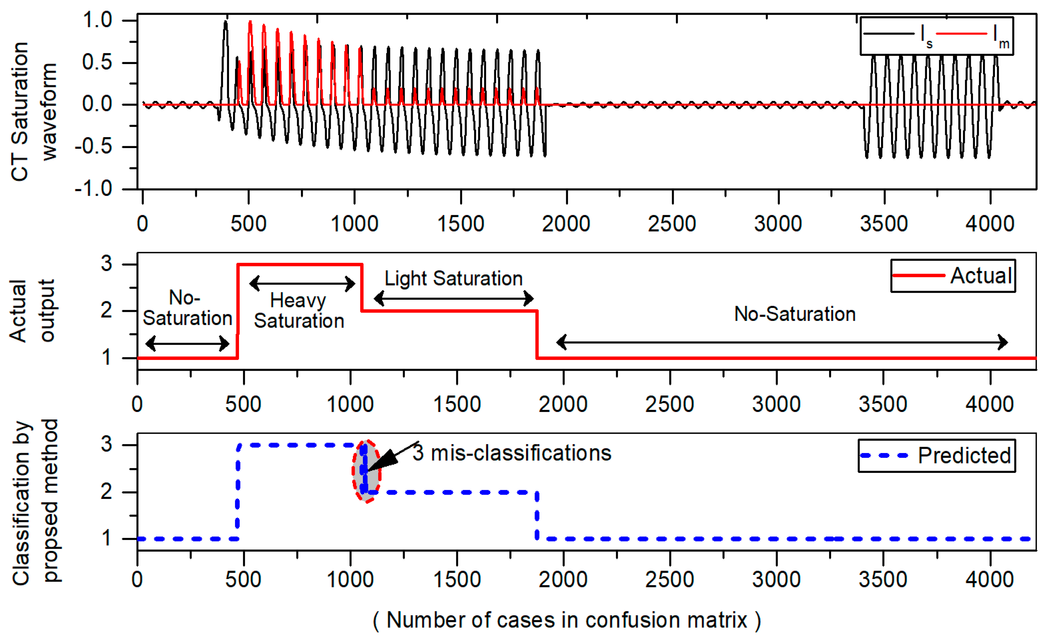
To assess the performance of a classification model for each class, we simulated different cases of CT saturation and results are displayed in confusion matrix as shown in
Table 7. The results of confusion matrix are then displayed with the waveform in
Figure 9 to visualize the number of misclassifications graphically. In confusion matrix, the green cells show the correctly classified cases whereas red cells indicate the number of misclassified cases. The yellow cell in the bottom right of the table shows the overall accuracy. The actual class is taken directly from original test dataset whereas predicted class values are obtained from the classifier on the test dataset. The description of three classes in confusion matrix is given as:
Results of
Table 7 show that that class 1 (No-saturation), and class 2 (light saturation) are classified successfully without any misclassifications. However, in the case of class 3 (heavy saturation), it has 584 samples in the test dataset, and only three cases are misclassified as class 2 (light saturation). Furthermore, the number of misclassifications in confusion matrix are also presented with CT saturation waveform as shown
Figure 9. Only three misclassifications are found which are encircled with red color. In
Table 7, the three diagonal cells in green color demonstrate the number of correct classifications by the trained network. For example, 2813 cases belonging to class 1 are correctly classified as No-saturation regions. Likewise, 819 and 581 cases belonging to class “2”, “3” are correctly classified as light and heavily saturated regions respectively. Only three misclassifications were noticed, while rest of the cases are correctly classified with a high accuracy of 99.93%. This analysis not only provides us with a way where mistakes are made, but it also provides a feasible way to increase the model performance.
Classification accuracy itself is typically not enough evidence to decide where your designed model is good enough to make robust predictions. The problem with accuracy is that it cannot discriminate among diverse kinds of misclassifications. So, additionally, we computed other performance metrics like precision, recall, specificity, F1-score, MCC [
38] by means of the confusion matrix. These terms are normally defined for binary classification problems where the outcome is either “positive” or “negative”. As, we have three classes and dealing with the multi-class problem, so we computed, precision, recall, F1-score, etc. while calculating TN, TP, FP, and FN of each class separately. A cleaner representation with different colors is shown in
Table 8, where various performance measures were obtained from the confusion matrix.
From
Table 8, it can be clearly seen that out of three classes “1”, “2” and “3”, each class has different FP and FN values. For example, for class “1” FP and FN are highlighted with light blue and pink color. Likewise, light green and dark green boxes show TP and TN for class “1” respectively. Now, with the application of these calculated TN, TP, FP, FN, we extracted the information of other performance measures for each class separately. For instance, performance metrics for class 1 (No-saturation) were calculated in
Table 9.
As illustrated in
Table 9, every performance metrics have different color representation which was extracted from confusion matrix of
Table 8. For example, accuracy is the proportion of correctly classified cases to a total number of cases. It was calculated as
Similarly, other performance metrics have been computed using the color scheme in
Table 9. Besides accuracy, we also calculated precision measure as it uncovers the differences in performance that go unobserved when using accuracy. It is the ratio of TP divided by FP and TP. On the other hand, recall is the ratio of TP divided by the number of TP and the FN. It is also termed as Sensitivity. Recall is another popular term which shows classifiers completeness. A small value of recall specifies many false negatives. Extending the previous results of precision and recall, we calculated another performance measure known as the F1-score. It is the weighted average of both precision and recall. Lastly, MCC was calculated, which is a best off-the-shelf evaluating tool for classification tasks. Performance of the proposed method on each class is recorded in
Table 10.
From
Table 10, it is interesting to see that; no misclassifications have been noted in class 1. Only few misclassifications were observed in case of class 2 and 3. Importantly, all these performance metrics were calculated from the confusion matrix. The results of
Table 10 indicate that our proposed method achieved significant performance on widely accepted performance metrics that include accuracy, precision, recall, specificity, F-score, and MCC. All CT saturation classes are classified correctly with relative high accuracy.
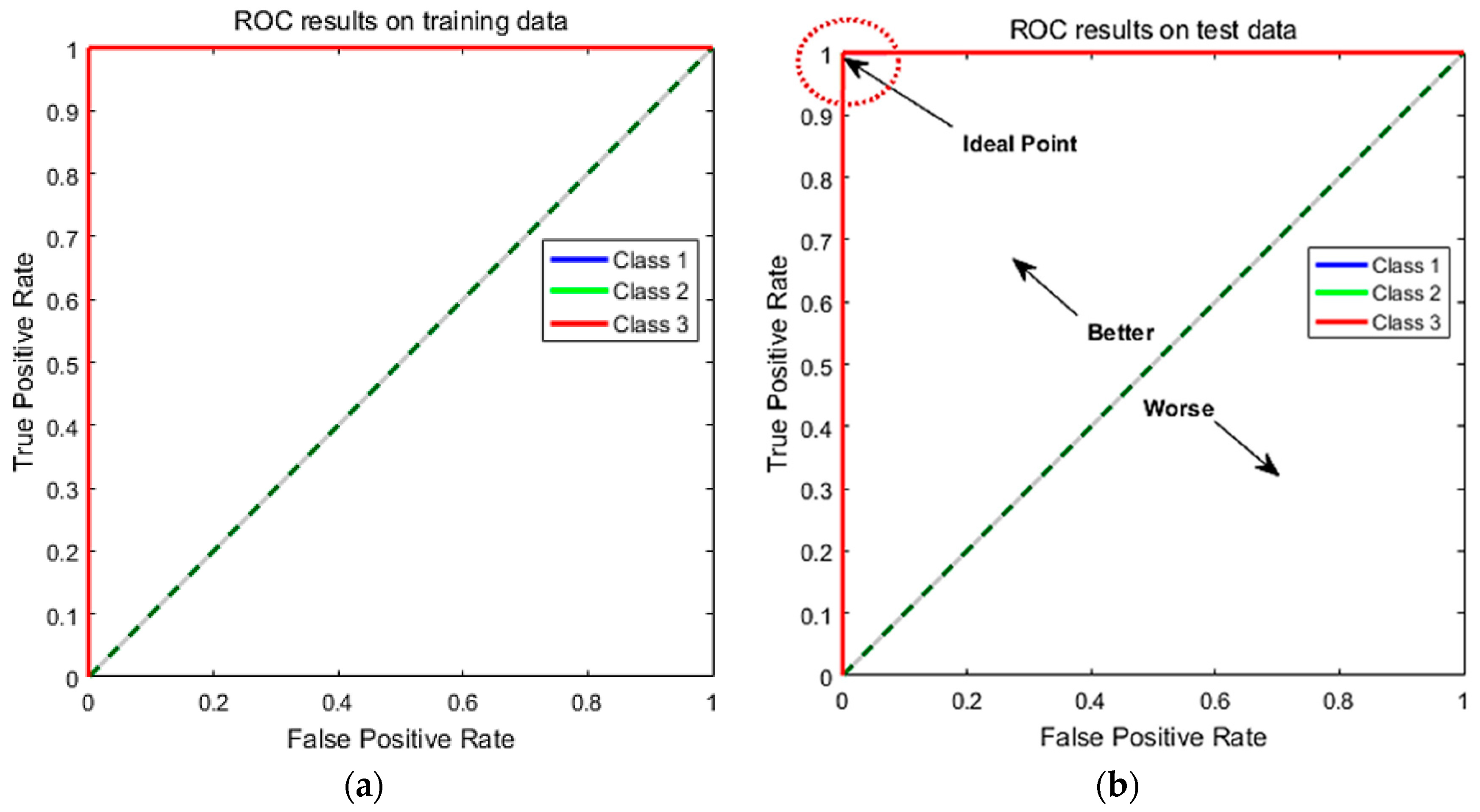
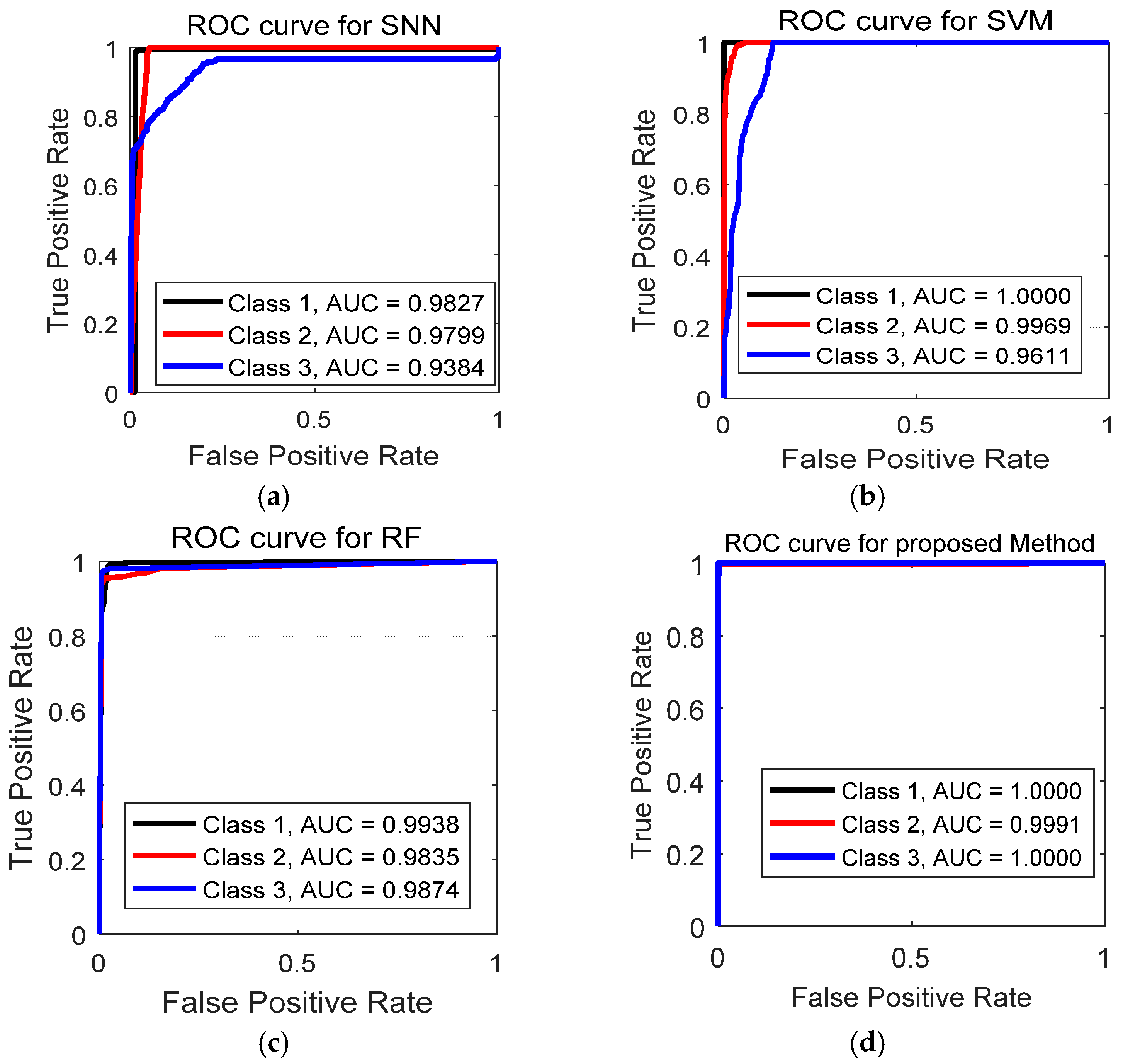
6.5. Performance Analysis Using Receiver Operating Characteristic (ROC) Curves
ROC Curve is an excellent technique for visualizing the performance based on their classification accuracy. Recently, these curves are heavily used by researchers due to their decision making abilities in classification problems [
39]. To extend ROC curve for multiclass classification, we have binarized the outputs. One ROC curve has been drawn per class. Compared to recall, precision, and F1 score, ROC curves solely depict a relationship between false positives rate (FPR) and true positive rate (TPR). The ROC curve is generated by plotting the FPR on the x-axis against the TPR on the
y-axis as shown in
Figure 10.
In
Figure 10, we have shown the obtained results for both training set and test set. The TPR on y-axis describes the number of positive cases that were correctly identified during the test. Whereas, FPR on x-axis defines the number of positive cases that were incorrectly classified as negative during the test. The diagonal line indicates the baseline. The ideal ROC curves should be above the diagonal. In general, models with ROC curves touching the top left corner of the ROC curve indicates better classification performance. The best point on the curve would be (0, 1), where all positive cases are classified correctly, and no negative cases are misclassified as positive. From
Figure 10a,b, we can see that both training and test curves touch the upper left corner (0, 1), which indicates a perfect classification on both training and test set. All the three levels of CT saturation (no saturation, light and heavy saturation) were classified successfully. The obtained ROC results validate that suggested method achieved accurate results for CT saturation classification.
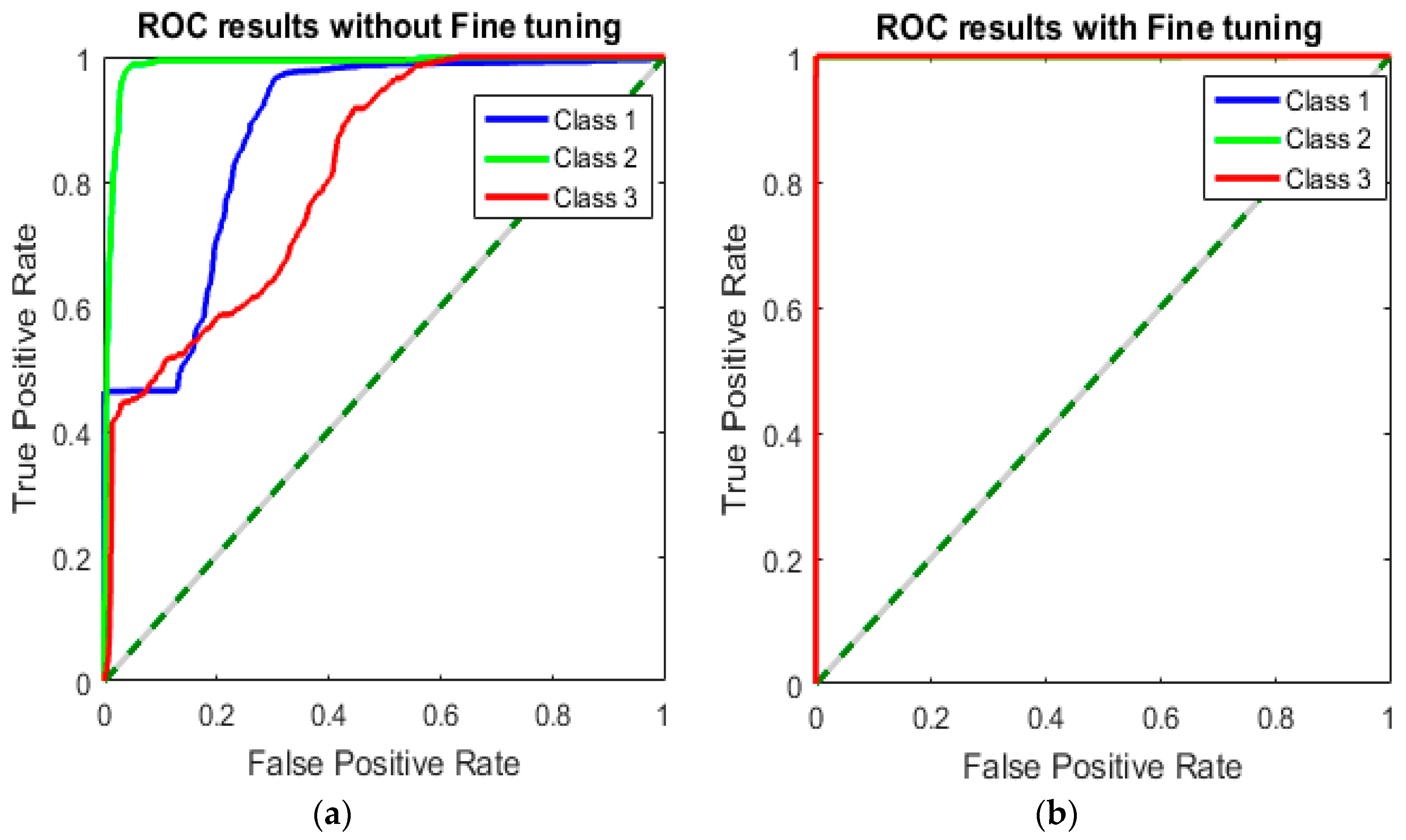
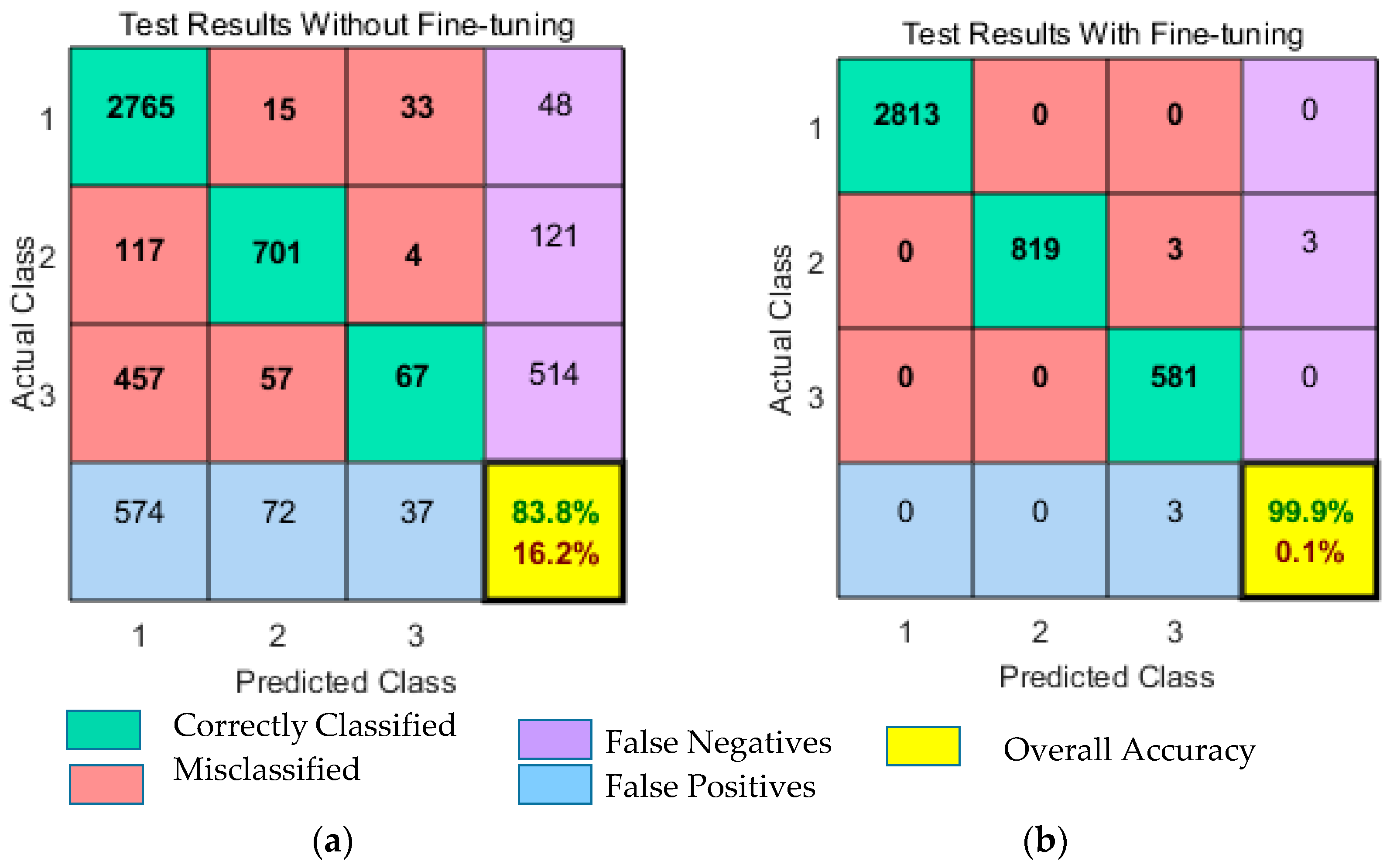
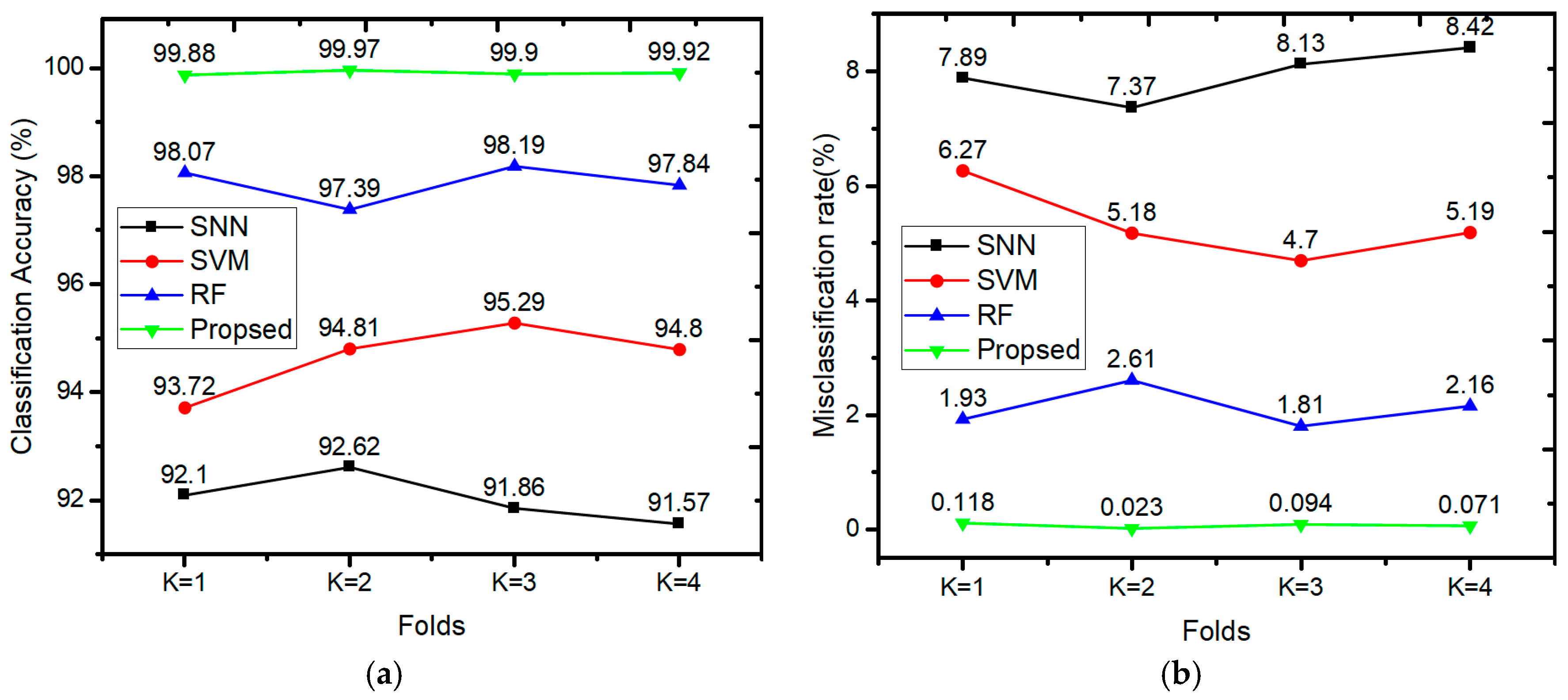
6.6. Results With Fine-Tuning Strategy
To observe the influence of fine-tuning strategy on classification performance, we compared the results with fine-tuning and without a fine-tuning strategy. As discussed previously in
Section 5, we have implemented the fine-tuning strategy in our work to improve performance even further. The results obtained from both fine-tuning and without fine-tuning are presented in
Figure 11 and
Figure 12. Remarkably, fine-tuning approach improves classification results by achieving an overall accuracy of 99.9%. Misclassification rate was only 0.1%. The classification accuracy without using the fine-tuning strategy was 83.8%, of which 13.8% was the misclassification rate. The obtained classification results and error rates are presented in
Table 11. From the table results, we can see that fine-tuning reduces the training error and improves the classification performance of DNN. The fine-tuning strategy not only improves the network performance but also contributes to obtain discriminative features for CT saturation classification. Moreover, the results displayed in
Figure 12 show that ROC curves without fine-tuning are far away from the upper left corner (0, 1). This indicates a poor classification performance with high misclassification rate. However, ROC curves with fine-tuning touch the ideal point (0, 1), which indicates the perfect classification.
The presented results in
Figure 11 and
Figure 12, concludes that fine-tuning strategy brought a significant improvement in classification accuracy and achieved state-of-the-art performance for CT saturation classification.


