Diagnosis Method for Li-Ion Battery Fault Based on an Adaptive Unscented Kalman Filter


Abstract
:1. Introduction
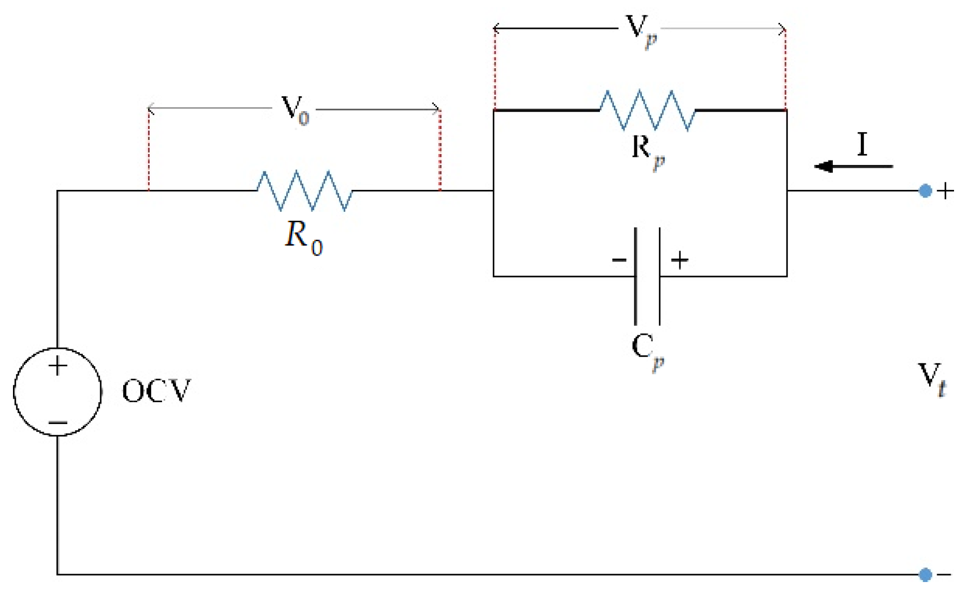
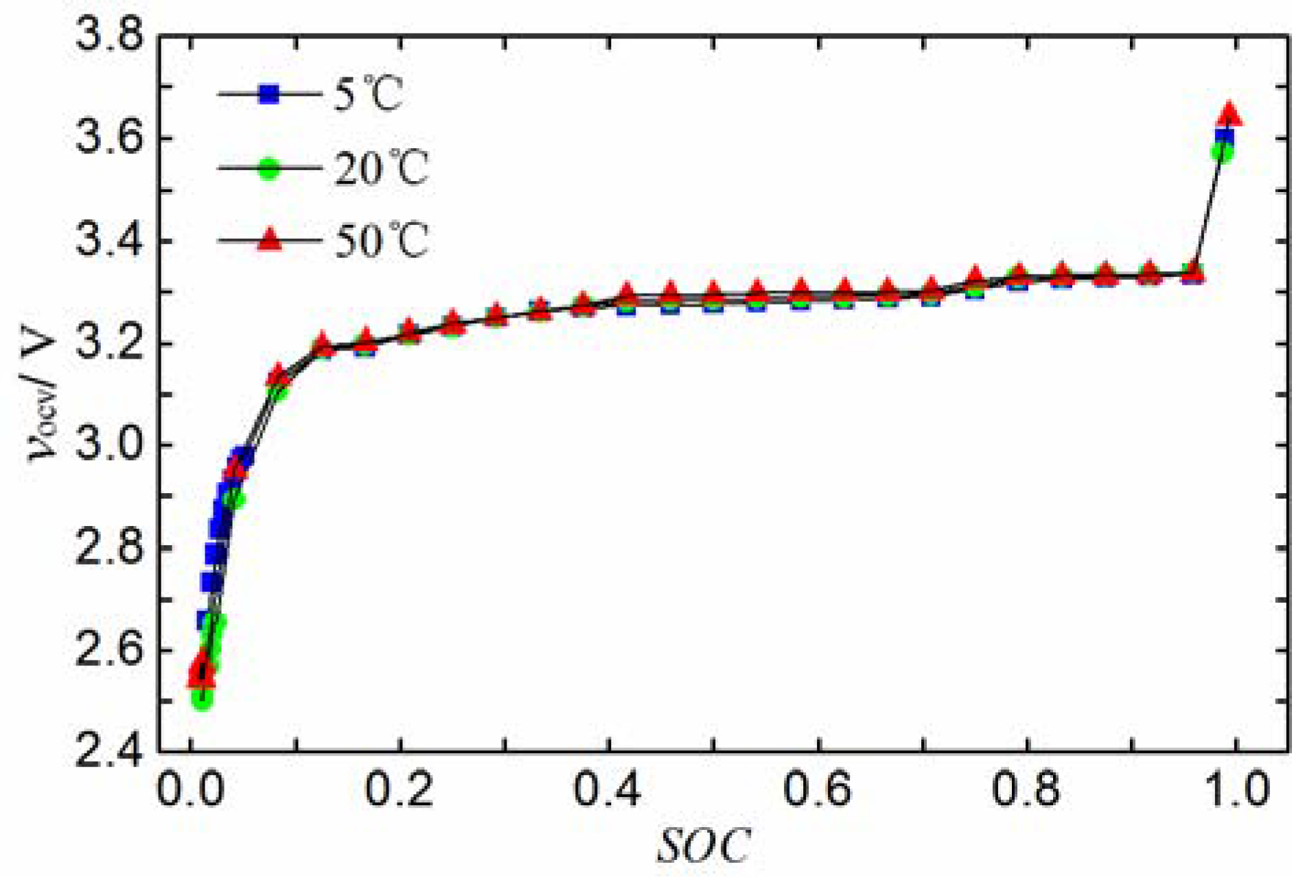
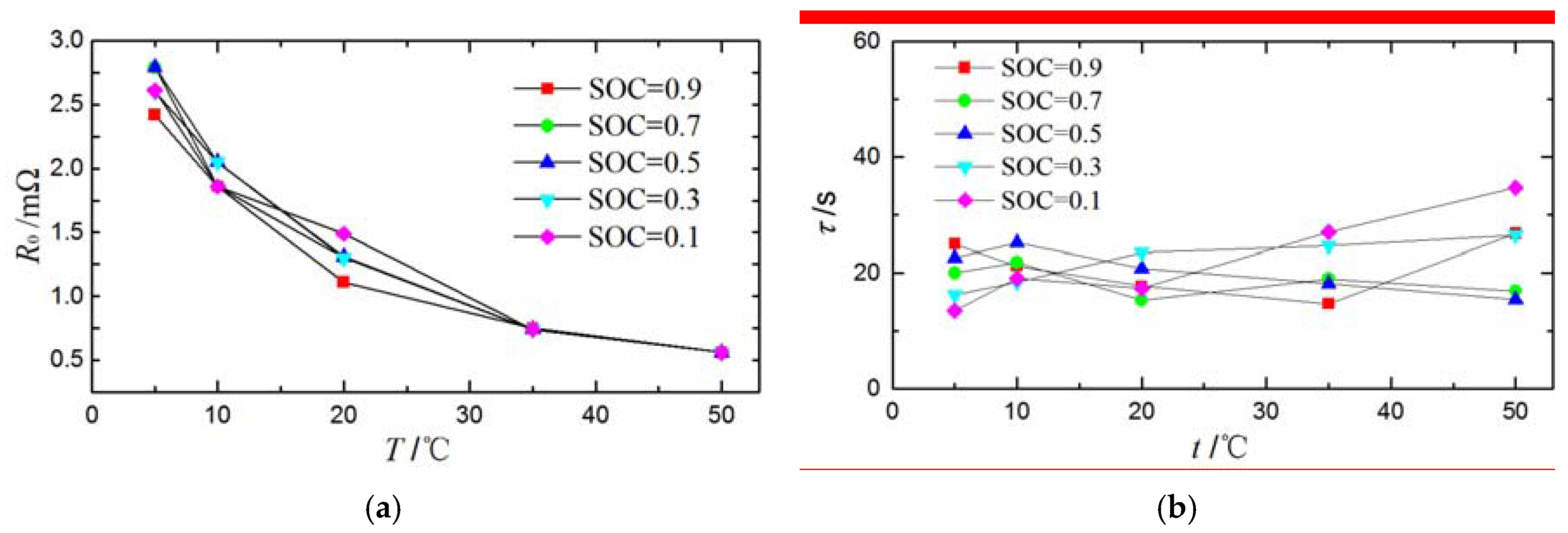
2. Battery Modeling
3. Parameters Estimation
3.1. Joint State Space Description
3.2. Joint Estimation Approach
| Algorithm 1. Details of the Adaptive Unscented Kalman Filter (AUKF) Algorithm |
| Step 1: Initialize Initializing estimated state value and covariance matrix . Step 2: Predict State and output Transform Sigma points to through (5), one-step estimate state , and covariance matrix . Modify the prediction of the covariance matrix: Step 3: Update state |
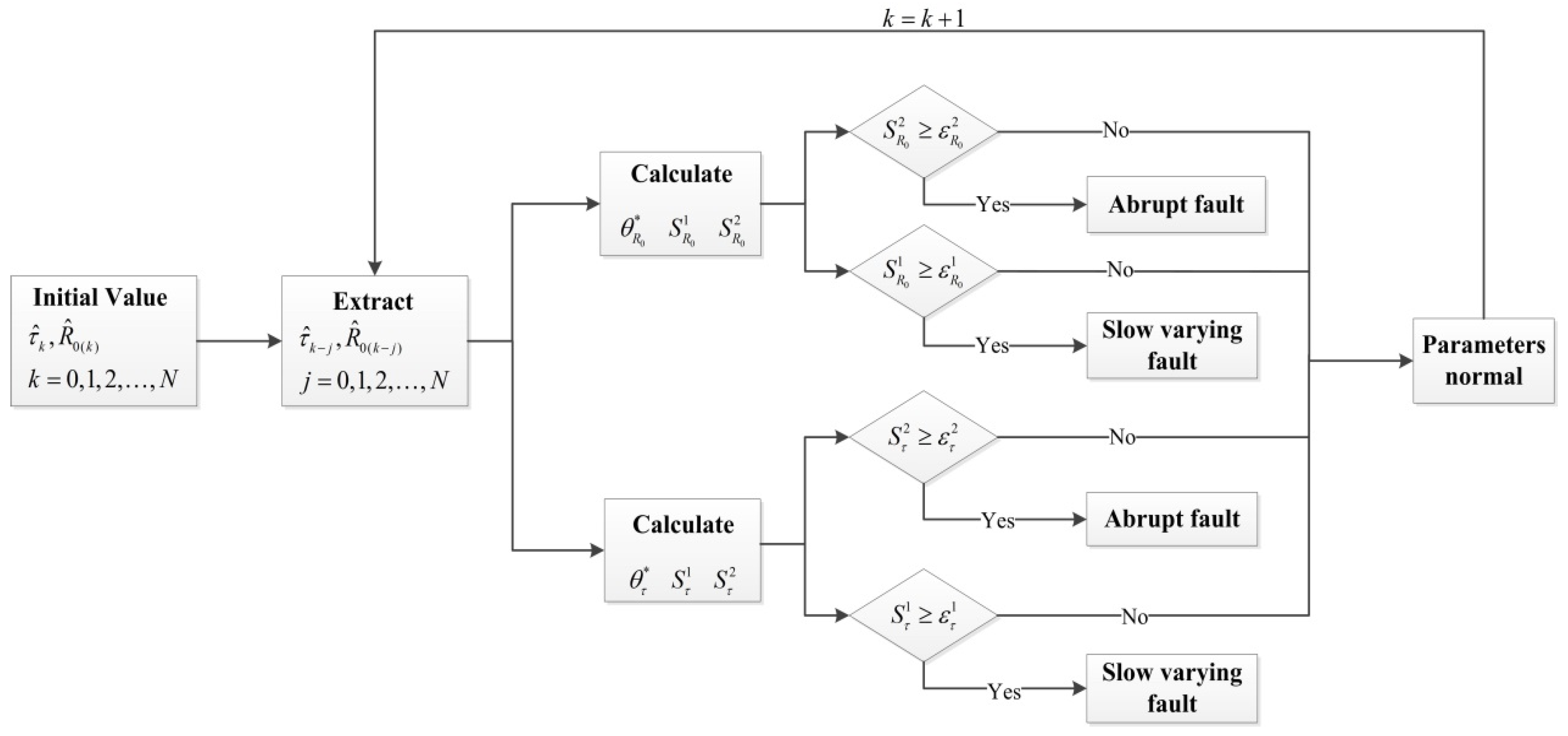
4. Diagnosis Approach for Parameter Bias Fault
- Step 1: Set a sequence of parameters within a data window ;
- Step 2: Extract and from the sequence;
- Step 3: Calculate , , and , , , respectively;
- Step 4: Start fault detection to detect the faults. If there is a fault, the detector alerts the system and breaks out; if there is no fault, the system moves to k + 1.
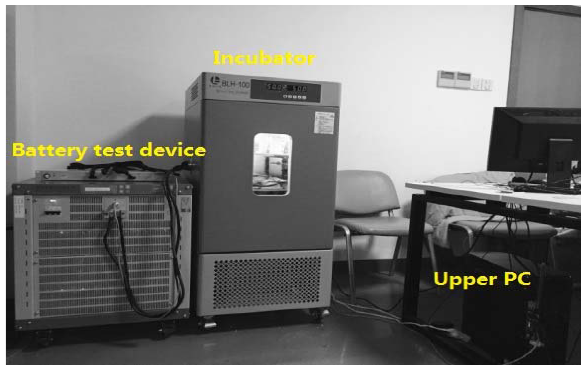
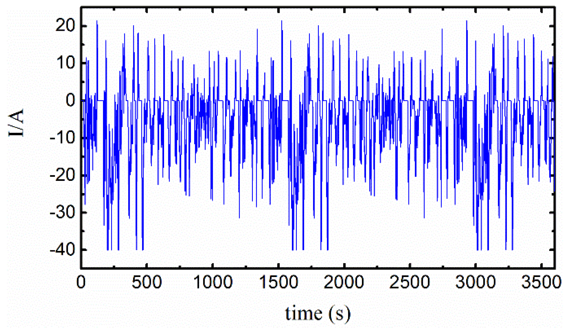
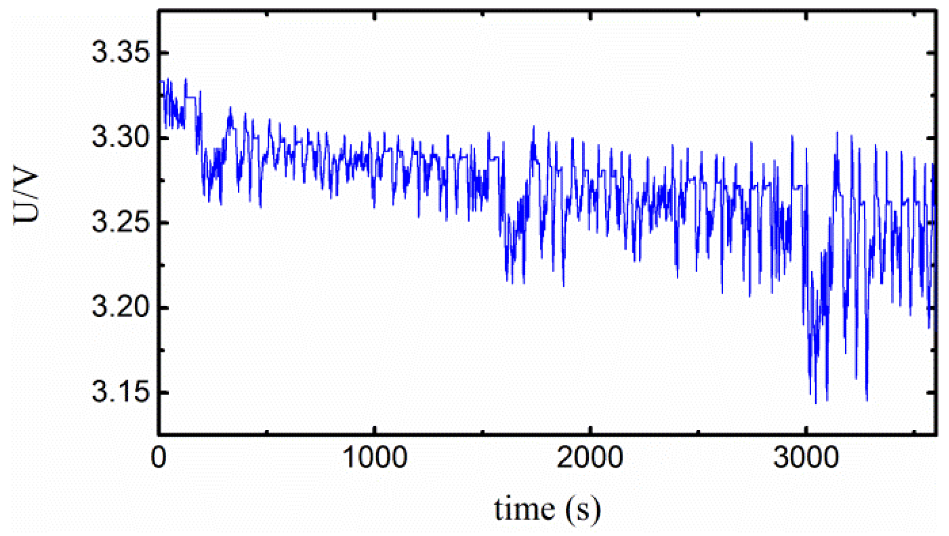
5. Experimental Validation
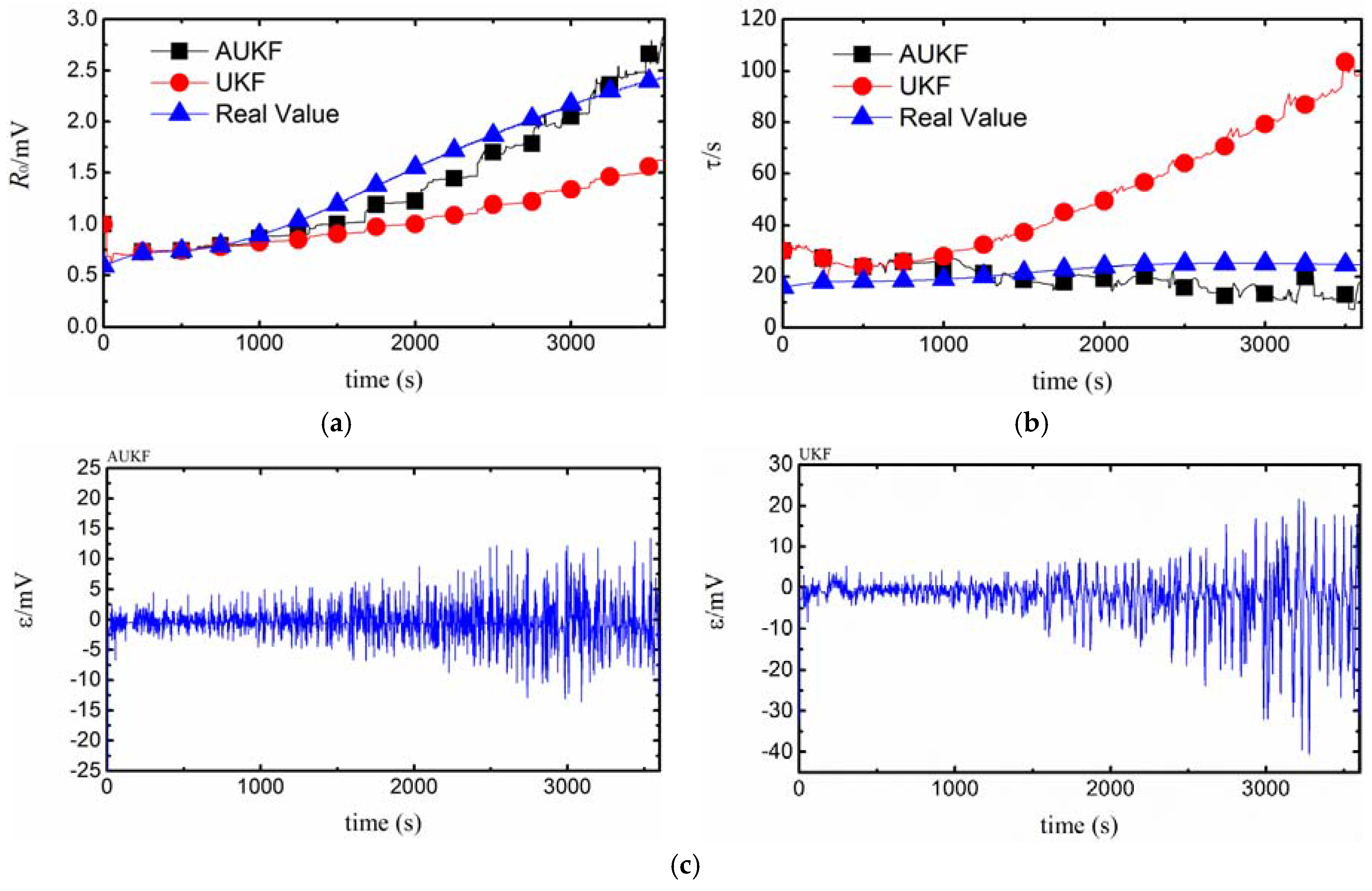
5.1. Diagnosis of Slow-Varying-Type Fault
5.2. Diagnosis of Abrupt Type Fault
6. Conclusions
Acknowledgments
Author Contributions
Conflicts of Interest
References
- Andrea, D. Battery Management Systems for Large Lithium-Ion Battery Packs; Artech House: Norwood, MA, USA, 2010. [Google Scholar]
- Sidhu, A.; Izadian, A.; Anwar, S. Adaptive nonlinear model-based fault diagnosis of Li-ion batteries. IEEE Trans. Ind. Electron. 2015, 62, 1002–1011. [Google Scholar] [CrossRef]
- Xia, B.; Shang, Y.; Nguyen, T.; Mi, C. A correlation based fault detection method for short circuits in battery packs. J. Power Sources 2017, 337, 1–10. [Google Scholar] [CrossRef]
- Chen, W.; Chen, W.T.; Saif, M.; Li, M.F.; Wu, H. Simultaneous fault isolation and estimation of lithium-ion batteries via synthesized design of Luenberger and learning observers. IEEE Trans. Control Syst. Technol. 2014, 22, 290–298. [Google Scholar] [CrossRef]
- Chen, Z.; Lin, F.; Wang, C.S.; Wang, L.Y.; Xu, M. Active diagnosability of discrete event systems and its application to battery fault diagnosis. Int. J. IEEE Trans. Control Syst. Technol. 2014, 22, 1892–1898. [Google Scholar] [CrossRef]
- Zhang, X.; Wang, Y.; Yang, D.; Chen, Z. An on-line estimation of battery pack parameters and state-of-charge using dual filters based on pack model. Energy 2016, 115, 219–229. [Google Scholar] [CrossRef]
- He, H.; Xiong, R.; Zhang, X.; Sun, F.; Fan, J.X. State-of-charge estimation of the lithium-ion battery using an adaptive extended Kalman filter based on an improved Thevenin model. IEEE Trans. Veh. Technol. 2011, 60, 1461–1469. [Google Scholar]
- Liu, L.; Wang, L.Y.; Chen, Z.; Wang, C. Integrated system identification and state-of-charge estimation of battery systems. IEEE Trans. Energy Convers. 2013, 28, 12–23. [Google Scholar] [CrossRef]
- Liu, X.; Chen, Z.; Zhang, C.; Wu, J. A novel temperature-compensated model for power Li-ion batteries with dual-particle-filter state of charge estimation. Appl. Energy 2014, 123, 263–272. [Google Scholar] [CrossRef]
- Sun, F.; Xiong, R. A novel dual-scale cell state-of-charge estimation approach for series-connected battery pack used in electric vehicles. J. Power Sources 2015, 274, 582–594. [Google Scholar] [CrossRef]
- Sun, F.; Xiong, R.; He, H. A systematic state-of-charge estimation framework for multi-cell battery pack in electric vehicles using bias correction technique. Appl. Energy 2016, 162, 1399–1409. [Google Scholar] [CrossRef]
- Dong, G.; Wei, J.; Zhang, C.; Chen, Z. Online state of charge estimation and open circuit voltage hysteresis modeling of LiFePO 4 battery using invariant imbedding method. Appl. Energy 2016, 162, 163–171. [Google Scholar] [CrossRef]
- Wang, Y.; Zhang, C.; Chen, Z. On-line battery state-of-charge estimation based on an integrated estimator. Appl. Energy 2015, 185, 2026–2032. [Google Scholar] [CrossRef]
- Zhang, C.; Wang, L.Y.; Li, X. Robust and adaptive estimation of state of charge for lithium-ion batteries. IEEE Trans. Ind. Electron. 2015, 62, 4948–4957. [Google Scholar] [CrossRef]
- Rahimi-Eichi, H.; Baronti, F.; Chow, M.Y. Online adaptive parameter identification and state-of-charge coestimation for lithium-polymer battery cells. IEEE Trans. Ind. Electron. 2014, 61, 2053–2061. [Google Scholar] [CrossRef]
- Chen, Z.; Wang, L.Y.; Yin, G.; Wang, C. Accurate Probabilistic Characterization of Battery Estimates by Using Large Deviation Principles for Real-Time Battery Diagnosis. IEEE Trans. Energy Convers. 2013, 28, 860–870. [Google Scholar] [CrossRef]
- Zhang, H.; Pei, L.; Sun, J.; Song, K.; Lu, R.; Zhao, Y. Online Diagnosis for the Capacity Fade Fault of a Parallel-Connected Lithium Ion Battery Group. Energies 2016, 9, 387. [Google Scholar] [CrossRef]
- Zheng, Y.; Han, X.; Lu, L.; Li, J.; Ouyang, M. Lithium ion battery pack power fade fault identification based on Shannon entropy in electric vehicles. J. Power Sources 2013, 223, 136–146. [Google Scholar] [CrossRef]
- Satadru, D.; Ayalew, B. A diagnostic Scheme for Detection, Isolation and Estimation of Electrochemical Faults in Lithium-ion Cells. In Proceedings of the ASME Annual Dynamic Systems and Control Conference, Columbus, OH, USA, 28–30 October 2015; p. 43. [Google Scholar]
- Dey, S.; Mohon, S.; Pisu, P.; Ayalew, B.; Onori, S. Online state and parameter estimation of Battery-Double Layer Capacitor Hybrid Energy Storage System. In Proceedings of the 54th IEEE Conference on Decision and Control, Osaka, Japan, 15–18 December 2015; pp. 676–681. [Google Scholar]
- Jim, M.; Onori, S.; Rizzoni, G. Nonlinear Fault Detection and Isolation for a Lithium-Ion Battery Management System. In Proceedings of the ASME Dynamic Systems and Control Conference, Cambridge, MA, USA, 12–15 September 2010; pp. 607–614. [Google Scholar]
- Zhou, D.H.; Su, Y.X.; Xi, Y.G.; Zhang, Z.J. Extension of Friedland’s separate-bias estimation to randomly time-varying bias of nonlinear systems. IEEE Trans. Autom. Control 1993, 38, 1270–1273. [Google Scholar] [CrossRef]
- Wang, X.X.; Zhao, L.; Xia, Q.X.; Hao, Y. Strong tracking filter based on unscented transformation. Control Decis. 2010, 25, 1063–1068. [Google Scholar]
- Sun, G.Q.; Huang, M.Y.; Wei, Z.N.; Sun, Y.; Zang, H. Dynamic State Estimation for Synchronous Machines Based on Unscented Transformation of Strong Tracking Filter. Proc. CSEE 2016, 36, 615–623. [Google Scholar]
- Hu, G.G.; Liu, Y.H.; Gao, S.S.; Yang, Y. Improved strong tracking UKF and its application in INS/GPS integrated navigation. J. Chin. Inert. Technol. 2014, 22, 634–639. [Google Scholar]
- Zou, C.; Manzie, C.; Nešić, D. A Framework for Simplification of PDE-Based Lithium-Ion Battery Models. IEEE Trans. Control Syst. Technol. 2016, 24, 1594–1609. [Google Scholar] [CrossRef]
- Chiang, C.J.; Yang, J.L.; Cheng, W.C. Temperature and state-of-charge estimation in ultracapacitors based on extended Kalman filter. J. Power Sources 2013, 234, 234–243. [Google Scholar] [CrossRef]

| slow varying fault | |
| abrupt fault | |
| slow varying fault | |
| abrupt fault |
| Rated Capacity | 20 Ah |
| Max Charge Voltage | 3.65 V |
| Min discharge Voltage | 2.5 V |
| Charge Rate | 1 C |
| Continuous discharge Rate | 3 C |
| Item | Contact Fault | Diffusion Fault | ||
|---|---|---|---|---|
| AUKF | UKF | AUKF | UKF | |
| Detection time/s | 2311 | 3585 | - | 1748 |
| Diagnosis result | Faulty | Faulty | Normal | Normal |
| Real fault situation | Fault (1960 s) | Normal | ||
| Item | Contact Fault | Diffusion Fault | ||
|---|---|---|---|---|
| AUKF | UKF | AUKF | UKF | |
| Detection time/s | 1715 | - | 1380 | - |
| Diagnosis result | Faulty | Normal | Faulty | Normal |
| Real fault situation | Fault (1300 s) | Normal | ||
© 2017 by the authors. Licensee MDPI, Basel, Switzerland. This article is an open access article distributed under the terms and conditions of the Creative Commons Attribution (CC BY) license (http://creativecommons.org/licenses/by/4.0/).
Share and Cite
Zheng, C.; Ge, Y.; Chen, Z.; Huang, D.; Liu, J.; Zhou, S. Diagnosis Method for Li-Ion Battery Fault Based on an Adaptive Unscented Kalman Filter. Energies 2017, 10, 1810. https://doi.org/10.3390/en10111810
Zheng C, Ge Y, Chen Z, Huang D, Liu J, Zhou S. Diagnosis Method for Li-Ion Battery Fault Based on an Adaptive Unscented Kalman Filter. Energies. 2017; 10(11):1810. https://doi.org/10.3390/en10111810
Chicago/Turabian StyleZheng, Changwen, Yunlong Ge, Ziqiang Chen, Deyang Huang, Jian Liu, and Shiyao Zhou. 2017. "Diagnosis Method for Li-Ion Battery Fault Based on an Adaptive Unscented Kalman Filter" Energies 10, no. 11: 1810. https://doi.org/10.3390/en10111810
APA StyleZheng, C., Ge, Y., Chen, Z., Huang, D., Liu, J., & Zhou, S. (2017). Diagnosis Method for Li-Ion Battery Fault Based on an Adaptive Unscented Kalman Filter. Energies, 10(11), 1810. https://doi.org/10.3390/en10111810