Identification of Combined Power Quality Disturbances Using Singular Value Decomposition (SVD) and Total Least Squares-Estimation of Signal Parameters via Rotational Invariance Techniques (TLS-ESPRIT)

Abstract

In order to identify various kinds of combined power quality disturbances, the singular value decomposition (SVD) and the improved total least squares-estimation of signal parameters via rotational invariance techniques (TLS-ESPRIT) are combined as the basis of disturbance identification in this paper. SVD is applied to identify the catastrophe points of disturbance intervals, based on which the disturbance intervals are segmented. Then the improved TLS-ESPRIT optimized by singular value norm method is used to analyze each data segment, and extract the amplitude, frequency, attenuation coefficient and initial phase of various kinds of disturbances. Multi-group combined disturbance test signals are constructed by MATLAB and the proposed method is also tested by the measured data of IEEE Power and Energy Society (PES) Database. The test results show that the new method proposed has a relatively higher accuracy than conventional TLS-ESPRIT, which could be used in the identification of measured data.

1. Introduction

With the switching-in of lots of non-linear and impact loads and the mass application of power electronic equipment, the power quality of distribution networks is becoming increasingly serious in recent years [1]. A single disturbance source could trigger a series of complex disturbances because of the increasing complexity of the grid [2]. Therefore, the accurate detection and recognition of power quality disturbances would be very helpful in the comprehension, evaluation and control of various kinds of power quality disturbances in power systems [3].

Nowadays, the ways to analyze power quality disturbances mainly focus on nonparametric methods and parametric methods. Nonparametric methods mainly rely on empirical mode decomposition (EMD) [4], short-time Fourier transform (STFT) [5], wavelet transform (WT) [6], and S-transform (ST) [7] as the way of feature extraction, and rely on neutral network (NN) [8], support vector machine (SVM) [9], decision tree (DT) [10], and fuzzy logic (FL) [11] as the disturbance classifiers. As to nonparametric methods, the upper limit of the disturbances classification accuracy is determined by the selected features, and the extent classification accuracy approximating upper limit is determined by the classifier. The application of nonparametric methods is slightly more difficult than it of parametric methods, as each combined disturbance whose element and extent are different could generate a new type. Also, the degree of disturbance is difficult to quantify.

Parametric methods include fast Fourier transform (FFT) [12], STFT [13], WT [14], Hilbert Huang transform (HHT) [15], Prony [16], matrix pencil method (MPM) [17], Kalman filter (KF) [18], sparse signal decomposition (SSD) [19], and local mean decomposition (LMD) [20]. These methods aim at completely extracting disturbance parameters as far as possible, then judging the type and degree of disturbance. Through parametric method, quantitative analysis can also be exerted on disturbance, with a clear standard. Therefore, these are appropriate for the recognition of complex disturbances.

Although FFT and STFT can accurately extract the frequency characteristics of disturbance sequences, they are not able to extract the transient behavior of the sequences [17,21]. All the methods based on EMD and LMD can decompose the signal into a set of intrinsic mode functions adaptively, but it is hard for the EMD method to distinguish the components whose frequencies are close [22]. End effect and mode aliasing also exist in both methods mentioned above, especially when dealing with time-varying sequences. WT is capable of decomposing the signal into a series of time-domain components and recognizing the abrupt information in the signal, but the number of decomposed layers and the choice of wavelet basis could have an uncertain influence on the decomposition results, and this method is also relatively sensitive to noise [23]. S-transform is the extension of STFT and the wavelet transformation method, which has strong noise immunity and doesn’t need to select basis functions, but this method has a high computation complexity O(N³) [24]. KF needs information about the measurement noise and an a priori harmonic model to estimate the linear system, but in practice, neither the harmonic model nor the noise statistics are known accurately [14]. SSD is based on sparse decomposition theory, which has a higher identification accuracy on complex signals, but the calculation of the dictionary is complicated, and it is easy for the applied greedy algorithm to accumulate error. Prony has been broadly applied in the field of extracting low-frequency oscillation parameters, which has a certain accuracy, but its calculation needs artificial order selection, which is closely related to recognition accuracy. In addition, as a global algorithm, Prony has a lower recognition accuracy on time-varying signals and the signals contain noise.

TLS-ESPRIT is a high-resolution subspace-based frequency estimating technique, it is robust to the noise [25], but not good at recognizing time-varying signals. Therefore, a method combining time-varying sequence segmentation, and high-resolution parameter estimating technique is proposed in this paper. Section 2 gives the characteristics of TLS-ESPRIT. A method based on SVD for identifying catastrophe points is proposed in Section 3. Simulation models are set up and experimental results are analyzed in Section 4. Finally, the conclusions are drawn in Section 5.

2. Parameters Identification by TLS-ESPRIT

2.1. TLS-ESPRIT

The sampling signal x(n) is supposed to be expressed by a group of attenuating sinusoidal component and white noise, as shown in (1):

$$x(n)={\displaystyle \sum _{i=1}^M{\alpha }_i}{z}_i^n+w(n)\mathrm{for}n=0,1,\cdots ,N-1$$

(1)

where ${\alpha }_i=\frac{a_i}{2}{e}^{j{\varphi }_i}$, $z_i=e^{(-{\xi }_i+j{\omega }_i)\mathsf{\Delta }t}$, ∆t is sampling interval, M is 2 times of p, which is the number of actual attenuating sinusoidal component. α_i, ξ_i, ω_i, φ_i are the amplitude, attenuation coefficient, angular frequency and initial phase of the ith attenuating sinusoidal component respectively. w(n) is the signal of white noise. The specific calculation flow is shown in [25].

2.2. Parameter Configuration

2.2.1. Model Order

The incorrect model order severely affects the parameter estimation by the subspace-based methods, as mentioned in [26]. Noise subspace is separated according to the singular value norm [27] as follows:

$$K_i={\left[\frac{{\sigma }_1^2+{\sigma }_2^2+\cdots +{\sigma }_i^2}{{\sigma }_1^2+{\sigma }_2^2+\cdots +{\sigma }_{L+1}^2}\right]}^{\frac{1}{2}}$$

(2)

where σ_i is the singular value of Hankel matrix for x(n). L is the number of columns in the Hankel matrix. When i changes from 1 to L + 1, K_i increases monotonously and gradually approaching 1. When:

$$K_i>\mu$$

(3)

all of the main information of original signal has been covered by the former i components, the rest components are detail information. Threshold μ is selected to be 0.995 based on a great deal of experimental verifies.

2.2.2. The Value of L

As to the value of L, in [28], it has been verified that the value of L plays an important role in suppressing noise interference. In this paper, er is assigned to the evaluation index which is the absolute value of relative error as shown in Equation (4), where $\widehat{x}$ is the fitted value, $x$ is actual value:

$$er=\frac{\left|\widehat{x}-x\right|}{x}\times 100\%$$

(4)

Considering both the timeliness of arithmetic and the identification precision of parameters, L is determined to be 3N/10.

2.2.3. The Minimum of N

(1) Rule 1

According to [25], it can be observed that V is a (L + 1) × (L + 1) orthogonal matrix, and V₁ is a (L + 1) × M subspace matrix of V, therefore:

$$M<L+1$$

(5)

The proper value of L is 3N/10, therefore:

$$M<\raisebox{1ex}{$3N$}\!\left/ \!\raisebox{-1ex}{$10$}\right.+1$$

(6)

In order to ensure a safe margin in actual application, the number of actual disturbance components is determined to be its maximum p_max = 10, namely M_max = 20. Thus, N should be greater than 64.

(2) Rule 2

In order to verify the influence of sampling frequency and the number of cycles for test signal on fitting accuracy, this test signal is adopted as:

$$x(n)=e^{-2n\mathsf{\Delta }t}\cos (100\pi n\mathsf{\Delta }t+\pi /3)+w(n)n=0,1,\dots ,\raisebox{1ex}{$f_{samp}$}\!\left/ \!\raisebox{-1ex}{$50$}\right.\times \alpha ,$$

(7)

where α is the number of cycles, value range is [0.1, 10], f_samp is the sampling frequency, value range is [1000, 6400], w(n) is the white noise, and SNR = 30 dB. Besides the relative error, reconstruction SNR is proposed to evaluate the similarities between fitting result and the actual signal:

$${\mathrm{SNR}}_{\mathrm{rec}}=10\times \lg \frac{{\displaystyle \sum _{n=1}^{N}x{(n)}^2}}{{\displaystyle \sum _{n=1}^N{[\widehat{x}(n)-x(n)]}^2}}$$

(8)

It can be seen from Figure 1 that the influence of sampling frequency is far less than the number of cycles. In addition, when lg(α) > −0.3, namely α > 0.5, the fitting errors of each parameter are low, and SNR_rec > 40 dB. Thus:

$$N>0.5\times \raisebox{1ex}{$f_{samp}$}\!\left/ \!\raisebox{-1ex}{$50$}\right..$$

(9)

In conclusion, the minimum of N is assigned to be the bigger one based on the proposed two rules.

3. Disturbance Location by SVD

3.1. Deficiency of TLS-ESPRIT

When the sequence has time-varying characteristics, namely the interval contains components with different starting and ending time, the error of order selection and parameter estimation will fluctuate along with its time-varying characteristics.

As shown in Equation (10), a group of test signals are constructed to simulate the time-varying component (150 Hz) accounting for different proportions in sequence, the sampling frequency is 6.4 kHz:

$$\begin{array}{ll}{x}_l(n)=& 5e^{-2n\mathsf{\Delta }t}\cos (100\pi n\mathsf{\Delta }t+\pi /3)+3e^{-(n-l)\mathsf{\Delta }t}u(n-l)\times \cos (300\pi n\mathsf{\Delta }t+\pi /4)\\ & l=0,1,\dots ,127\end{array}$$

(10)

It can be seen from Figure 2a that, when the length of time-varying component is 30 samples, the singular value norm method detects that the signal contains two different modes. Therefore, the boundary can be determined as 30, and the corresponding er graphs are draw in Figure 2b,c.

It is clear that when all components have the same starting and ending time, the fitting errors are the lowest. In summary, the locating of the disturbance at the beginning and ending time for parameters fitting is essential. Thus, a method based on SVD is proposed in Section 3.2 [29].

3.2. Disturbance Location by SVD

The Hankel is constructed matrix by the original signal x(n) as (11):

$$X={\left[\begin{array}{cccc}x(0)& x(1)& \dots & x(L)\\ x(1)& x(2)& \dots & x(L+1)\\ ⋮& ⋮& ⋮& ⋮\\ x(N-L-1)& x(N-L)& \dots & x(N-1)\end{array}\right]}_{(N-L)\times (L+1)}$$

(11)

where N is the length of the signal and L is the beam parameter.

SVD is performed on the constructed matrix as Equation (12):

$$X=U\mathsf{\Lambda }{V}^{\mathrm{T}}$$

(12)

where U is a (N − L) × (N − L) orthogonal matrix. $\mathsf{\Lambda }$ is a (N − L) × (L + 1) diagonal matrix, whose main diagonal element is the singular value of X, namely [σ₁, σ₂, ⋯, σ_L+1]. V is a (L + 1) × (L + 1) orthogonal matrix.

The above formula can be expanded as:

$$X={\sigma }_1{u}_1{v}_1^T+{\sigma }_2{u}_2{v}_2^T+\cdots +{\sigma }_m{u}_m{v}_m^T$$

(13)

where $u_i\in R^{(N-L)\times 1}$, $v_i\in R^{(L+1)\times 1}$, i = 1, 2, $\cdots$ m, m = L + 1.

Each component can be represented as:

$$X_i={\sigma }_i{u}_i{v}_{{}_i}^T\in R^{(N-L)\times (L+1)}$$

(14)

Furthermore:

$$X_i={\left[\begin{array}{cccc}{x}_{i,0}& x_{i,1}& \cdots & x_{i,L}\\ x_{i,1}& x_{i,2}& \cdots & x_{i,L+1}\\ ⋮& ⋮& ⋮& ⋮\\ x_{i,N-L-1}& x_{i,N-L}& \cdots & x_{i,N-1}\end{array}\right]}_{(N-L)\times (L+1)}$$

(15)

Equation (16) can be obtained by connecting the end of first row to the head of last column:

$$P_i=[x_{i,0},x_{i,2},\cdots x_{i,N-1}]$$

(16)

It is easy to prove that:

$$X={\displaystyle \sum _{i=1}^m{P}_i}$$

(17)

From P₁ to P_m are the main components, the abrupt information and the noise of original signal respectively. Simulation results show that when the value of L is large, the abrupt information is aliased with the main component. On the contrary, the abrupt information is aliased with the noise. Experimental results show that the decomposition is reasonable when L ranges from 15 to 30. Therefore, L is assigned as 20.

Singular value norm method is still used in this section to do discrimination, and the division basis is shown in Figure 3. Figure 3 is the simulation diagram of complex disturbance with oscillation and voltage flicker, the test function is shown as:

$$\begin{array}{ll}x(n)& =[1+0.5\cos (20\pi n\mathsf{\Delta }t+\pi /4)]\times [u(n-385)-u(n-1621)]\\ & \times \cos (100\pi n\mathsf{\Delta }t+\pi /3)+0.7e^{-10(n-100)\mathsf{\Delta }t}\times [u(n-100)-u(n-900)]\times \cos (1000\pi n\mathsf{\Delta }t+\pi /2)\\ & +[u(384-n)+u(n-1622)]\times \cos (100\pi n\mathsf{\Delta }t+\pi /3)\end{array}$$

(18)

It can be seen from the singular value norm in Figure 3 that the norm has exceeded the threshold 0.995 in the fourth layer. Therefore, the first four layers are the main signal components. Figure 3a is the waveform of P₁, which has geometric similarity with the original signal. The remaining layers are abrupt information and noise, Figure 3b is the waveform of P₅, and the locations of four catastrophe points are very clear. Figure 3d is the waveform of P₂₀, which can be considered as white noise. After the locating of abrupt information is completed, the data between the catastrophe points are extracted, and the algorithm flow is shown in Figure 4.

4. Simulations and Results

According to [30], power quality disturbances are divided into voltage sag, voltage swell, voltage interruptions, harmonics, transient pulse, interharmonics, voltage fluctuation, transient oscillation, frequency offset, voltage notches, voltage unbalance, DC offset, and noise. In this paper, MATLAB is used to simulate the combined disturbance, and the sampling frequency of simulation signal is 6.4 kHz, the signal-to-noise ratio is 30 dB. The proposed method are also validated by the measured data of IEEE PES Database [31].

4.1. Test Signal Constructed by MATLAB

4.1.1. Oscillation + Flicker

The test signal of the complex disturbance of oscillation and voltage flicker is shown in Equation (18). The disturbance interval is [101, 1621]. The data from half cycle before the starting time to the half cycle after the ending time of the disturbance signal are intercepted to identify catastrophe point, as shown in Figure 5.

From the singular value norm, it can be observed that the catastrophe point information exists in P₅. The catastrophe points are 101, 387, 902 and 1621, respectively, which differ little from the actual catastrophe points. The disturbance is divided according to the above-mentioned catastrophe points, and parameters are extracted from each interval. The orders of the intervals are 4, 8 and 6 respectively and the results are shown in

Table 1. Parameters identification of Equation (18).

Interval	f/Hz	a/p.u.	ξ	φ/rad
[101, 386]	49.9629	0.9978	−0.1046	0.3350π
	500.02	0.6960	9.7534	0.5008π
[387, 901]	39.6771	0.2531	0.4017	0.0873π
	50.1538	0.8945	−0.2551	0.3433π
	59.9075	0.2522	0.3234	0.5865π
	500.0101	0.4470	10.1213	0.5012π
[902, 1621]	39.8909	0.2496	0.1955	0.0921π
	50.0226	0.9985	0.0327	0.3291π
	60.0851	0.2492	−0.2091	0.5638 π

.

From Table 1, it can be found that 500 Hz oscillation occurred in the first interval. By the 40 Hz and 60 Hz components and Equation (19), it can be judged that the disturbance intervals are also mixed with 10 Hz voltage flicker, whose amplitude is about 0.5021:

$$\begin{array}{ll}x(t)& =[1+a\cos (2\pi f_{1}t+{\varphi }_1)]\times \cos (2\pi f_{2}t+{\varphi }_2)\\ & =\cos (2\pi f_{2}t+{\varphi }_2)+\frac{a}{2}\cos [2\pi (f_2-f_1)+({\varphi }_2-{\varphi }_1)]+\frac{a}{2}\cos [2\pi (f_2+f_1)+({\varphi }_2+{\varphi }_1)]\end{array}$$

(19)

Table 2. Comparative analysis of the proposed method, Prony method (order = 8), and the TLS-ESPRIT (order = 8)/%.

Component	f			a			ξ			φ
	M1	M2	M3	M1	M2	M3	M1	M2	M3	M1	M2	M3
40 Hz	0.540	0.152	-	0.560	38.880	-	0.299*	2.488 *	-	7.683	17.047	-
50 Hz	0.093	0.031	0.009	3.650	1.1602	8.870	0.109*	0.804 *	0 *	0.901	1.080	1.890
60 Hz	0.006	0.006	-	0.280	37.600	-	0.057*	2.403 *	-	1.443	1.881	-
500 Hz	0.003	0	0.468	0.571	3.514	57.743	0.626	23.620	100	0.200	0.580	26.100

The least error is marked in bold. * means absolute error. M₁: the proposed method, M₂: TLS-ESPRIT method, M₃: Prony method.

are the relative errors of each parameter for the disturbance described by Equation (18) using the proposed method, the TLS-ESPRIT with order of 8, and the Prony method with order of 8 respectively. Figure 6 shows the source disturbance with the reconstructed signals using three different methods mentioned above. As can be seen from the table, the recognition errors based on the Prony method are largest. Two components are not identified at all. The TLS ESPRIT-while recognizing all four kinds of component, but only the identification accuracy of 50 Hz component is higher, just because it is the main component of the signal and owns a weaker non-stationary property. It is obvious that the proposed method has the best performance on disturbance identification.

4.1.2. Harmonic + Sag with Phase Jump

The multiple disturbance power signal, which consists of 3th harmonic, 5th harmonic and voltage sag with phase jump, is constructed by MATLAB as shown in Equation (20):

$$\begin{array}{l}x(n)=\cos (100\pi n\mathsf{\Delta }t+\pi /3)\times [u(740-n)+u(n-1781)]+0.5\cos (100\pi n\mathsf{\Delta }t+\pi /2)\\ \times [u(n-741)-u(n-1780)]+0.5\cos (300\pi n\mathsf{\Delta }t+\pi /4)\times [u(n-321)-u(n-1501)]\\ +0.3\cos (500\pi n\mathsf{\Delta }t+\pi /3)\times [u(n-461)-u(n-1237)]\end{array}$$

(20)

The disturbance interval is [321, 1780]. Theabrupt information exists in P₅ as shown in Figure 7, and the catastrophe points are 321, 465, 743, 1240, 1501 and 1780, respectively. Intervals are divided based on the above points, and the model orders are 4, 6, 6, 4 and 2, respectively. The parameters are extracted from each interval and the results are shown in

Table 3. Parameter identification of Equation (20).

Interval	f/Hz	a/p.u.	ξ	φ/rad
[321, 465]	49.9063	0.9965	−0.2219	0.3292π
	149.9176	0.5048	−0.0913	0.2542π
[466, 743]	50.0497	1.0039	0.2085	0.3372π
	149.9177	0.4984	−0.1415	0.2581π
	250.2602	0.2982	0.4446	0.3381π
[744, 1242]	49.9960	0.5044	0.2346	0.5074π
	149.9865	0.4948	0.1244	0.2552π
	250.0624	0.3026	0.2235	0.3291π
[1243, 1505]	50.0766	0.4863	−0.0967	0.4979π
	150.0088	0.5063	0.3693	0.2475π
[1506, 1780]	50.0549	0.5018	0.3434	0.4970π

. From the data in Table 3, it can be seen that the disturbances contain 3th harmonic, 5th harmonic and voltage sag. According to the phase parameter between [466, 743] and [744, 1242], the voltage sag is accompanied by a 0.1702π rad phase jump.

Table 4. Comparative analysis of the proposed method, Prony method (order = 6), and the TLS-ESPRIT (order = 6)/%.

Component	f			a			ξ			φ
	M1	M2	M3	M1	M2	M3	M1	M2	M3	M1	M2	M3
50 Hz	0.044	1.338	1.320	0.020	8.940	31.560	0.007 *	5.390 *	0 *	0.030	133.423	168.360
50 Hz (sag)	0.085	-	-	0.500	-	-	0.460 *	-	-	0.160	-	-
150 Hz	0.028	0.040	4.882	0.220	16.040	206.040	0.111 *	3.173 *	0*	1.520	200.800	228.480
250 Hz	0.105	0.071	-	0.133	25.000	-	0.334 *	2.613 *	-	0.090	139.333	-

The least error is marked in bold.* means absolute error. M₁: the proposed method, M₂: TLS-ESPRIT method, M₃: Prony method.

lists the relative errors of each parameter for the disturbance described by Equation (20) using three different methods. Similarly, because of the non-stationary property of the signal, the TLS-ESPRIT and Prony method cannot recognize all the disturbances. For TLS-ESPRIT, only the 50 Hz component is identified, but the normal 50 Hz component and the 50 Hz sag component are confused. The Prony method has a worse performance. Even the 250 Hz component is not identified. The evaluation accuracies of the recognized components based on these two methods are much lower than the proposed method.

Figure 8 shows the source disturbance with the reconstructed signals using these three different methods. The reconstructed signal based on the proposed method almost completely coincide with the source disturbance.

4.1.3. Attenuation DC Offset + Interharmonic + Pulse

The power signal with attenuation DC offset, interharmonic and transient pulse is shown in Equation (21):

$$\begin{array}{l}x(n)=\cos (100\pi n\mathsf{\Delta }t+\pi /3)+0.4\times [u(n-791)-u(n-792)]+0.5\cos (212\pi n\mathsf{\Delta }t+\pi /4)\\ \times [u(n-321)-u(n-1601)]+0.6e^{-(n-642)\mathsf{\Delta }t}\times [u(n-642)-u(n-1433)]\end{array}$$

(21)

The disturbance interval is [321, 1601]. The abrupt information exists in P₅ as shown in Figure 9, and the catastrophe points are 321, 646, 793, 1438 and 1601, respectively. The orders of the disturbance intervals are 4, 5, 5 and 4, respectively. The parameters are extracted from each interval and the results are shown in

Table 5. Parameter identification of Equation (21).

Interval	f/Hz	a/p.u.	ξ	φ/rad
[321, 645]	49.9328	1.0016	−0.0423	0.3341π
	106.0592	0.4978	0.1152	0.2525π
[646, 791]	0	0.6048	1.0980	-
	50.0032	0.9998	−0.0024	0.3333π
	105.9941	0.5038	0.0466	0.2477π
[792, 1436]	0	0.5887	1.0729	-
	50.0069	1.0039	0.0646	0.33875π
	105.9837	0.5011	0.0420	0.25095π
[1437, 1601]	49.9899	1.0122	0.0804	0.3338π
	105.9590	0.4999	0.1213	0.2479π

. The attenuation DC offset and interharmonic can both be accurately identified.

The parameters of Table 5 are used to do signal reconstruction and then do subtraction with the original signal. Then difference operator is calculated as shown in Figure 10. It can be seen that at sample 791, there is still a pulse with an amplitude of 0.4336.

Table 6. Comparative analysis of the proposed method, Prony method (order = 5), and the TLS-ESPRIT (order = 5)/%.

Component	f			a			ξ			φ
	M1	M2	M3	M1	M2	M3	M1	M2	M3	M1	M2	M3
50 Hz	0.034	0.111	1.5706	0.440	15.570	25.550	0.025 *	1.583 *	0 *	0.510	1.410	48.515
106 Hz	0	0.943	-	0.140	7.240	-	0.081 *	0.525 *	-	0.080	4.320	-
DC offset	-	-	-	0.800	4.433	-	8.540	23.100	-	-	-	-
Impulse	0	-	-	0.084	-	-	-	-	-	-	-	-

The least error is marked in bold.* means absolute error. M₁: the proposed method, M₂: TLS-ESPRIT method, M₃: Prony method.

lists the relative errors of each parameter for disturbance described by Equation (21) using three different methods. The performance difference of TLS-ESPRIT and the proposed method is mainly reflected in DC offset. Figure 11 shows the source disturbance with the reconstructed signals using these three different methods.

4.2. Measured Data from IEEE PES Database

4.2.1. Case 1

In order to verify the practicability of the method, the measured data of IEEE PES Database is selected to do verification. The sampling frequency of the measured data is 12.8 kHz. It can be seen from Figure 12 that the disturbance begins at the 456th sample. The disturbance interval is divided into two segments, namely [456, 1140] and [1141, 1536], respectively. The identified parameters are shown in

Table 7. Parameters identification of case 1.

Interval	f/Hz	a/p.u.	ξ	φ/rad
[456, 1140]	49.0887	0.3643	11.7839	−0.6176
	81.1974	0.3886	175.1813	−0.5957
	378.8554	0.2257	561.2546	−0.4287
	2685.8132	0.2161	841.7556	0.0914
[1141, 1536]	48.8825	0.2126	16.8734	0.6766
	131.4223	0.0118	−30.7727	−2.5587
	1380.6588	0.1609	1505.9565	0.1363
	2500.3552	0.2572	2037.8554	−0.6680

.

It can be observed from the data in the Table 7 that the initial stages of the two disturbance intervals are accompanied by an instantaneous oscillation of more than 2.5 kHz, and the duration of attenuation is extremely short. The original 50 Hz signal has a voltage sag and is accompanied by a frequency offset. It can be seen from the attenuation coefficient and the amplitude parameters of the two intervals that the component is still in a state of constant attenuation, and the other interharmonic components have no obvious features, which does not need to be repeated.

4.2.2. Case 2

47 groups of single PQ events collected in a 220 kV substation are also selected, which are 19 groups of voltage sag, four groups of voltage sag + harmonic, six groups of voltage sag + oscillation, five groups of voltage swell, two groups of voltage swell + harmonic, two groups of flickering, three groups of oscillation, and six groups of harmonics. Due to the fact that the specific components of real world data are not accurately obtained in advance, the relative error cannot be chosen to evaluate the precision. In order to illustrate the effectiveness of the proposed method, SNRrec is used to evaluate the parameter identification results. The comparison with TLS-ESPRIT and Prony is also added and the box plot is drawn as shown in Figure 13, which could verify the practicability and superiority of the proposed method.

5. Conclusions

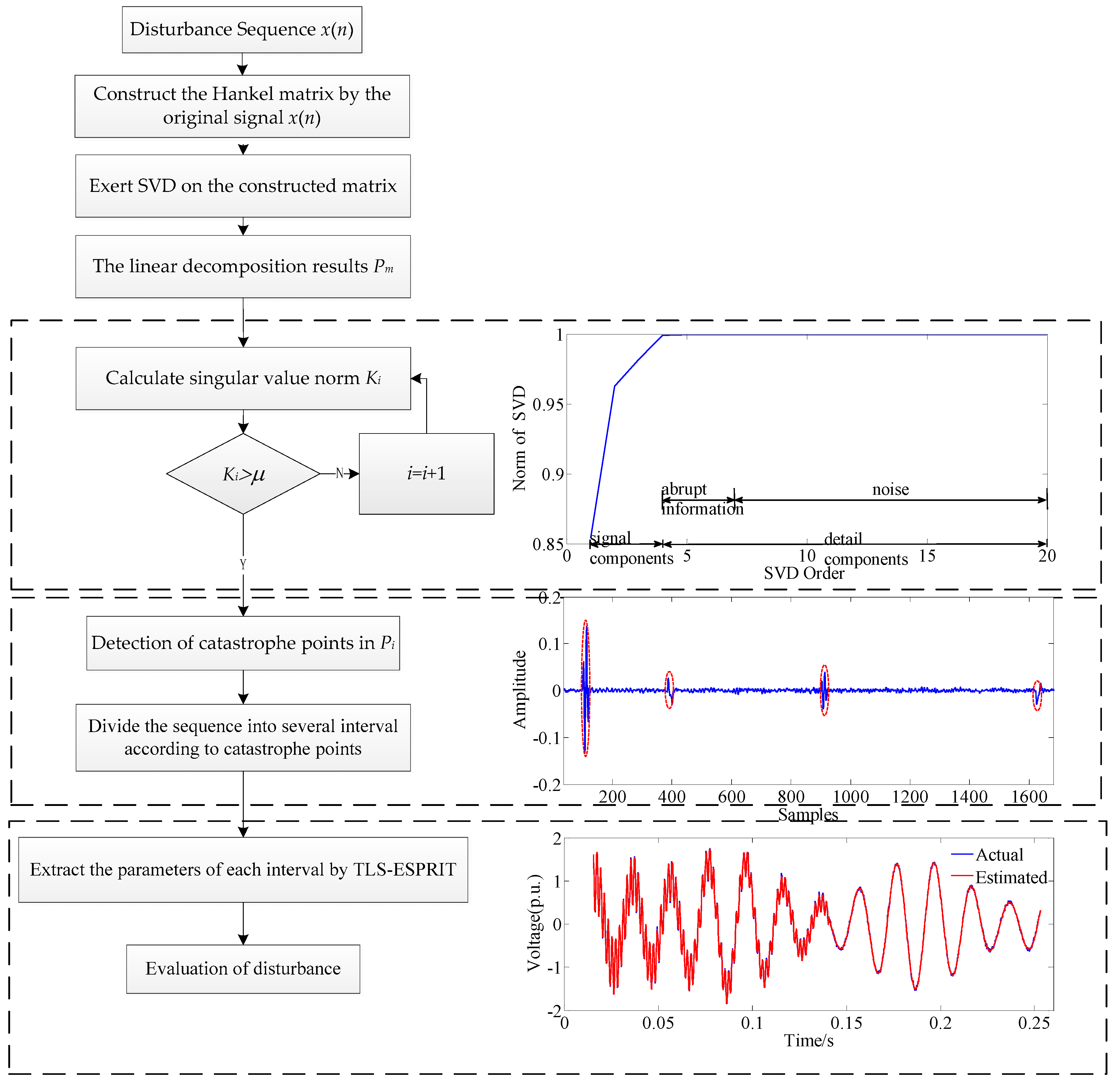
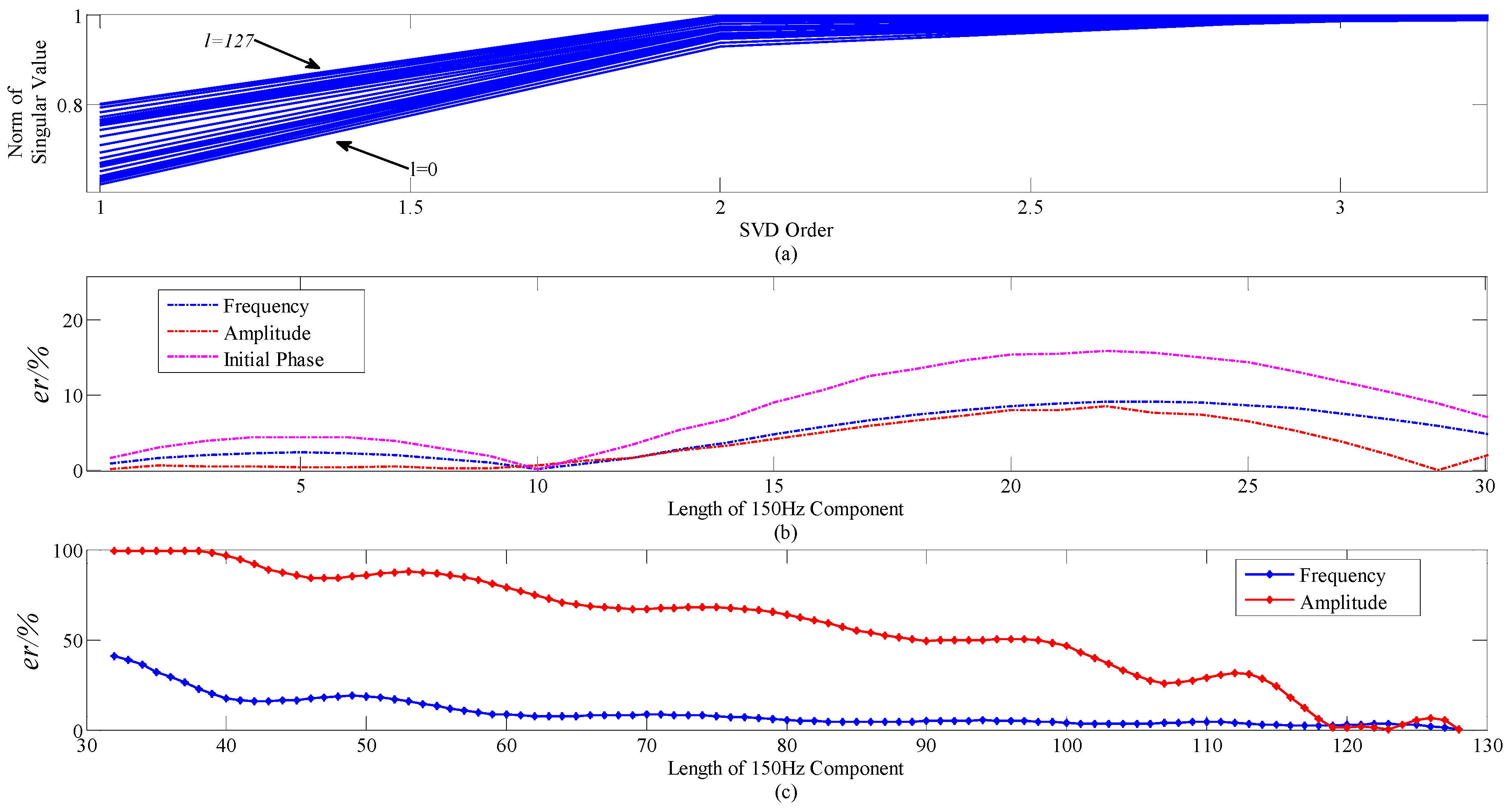
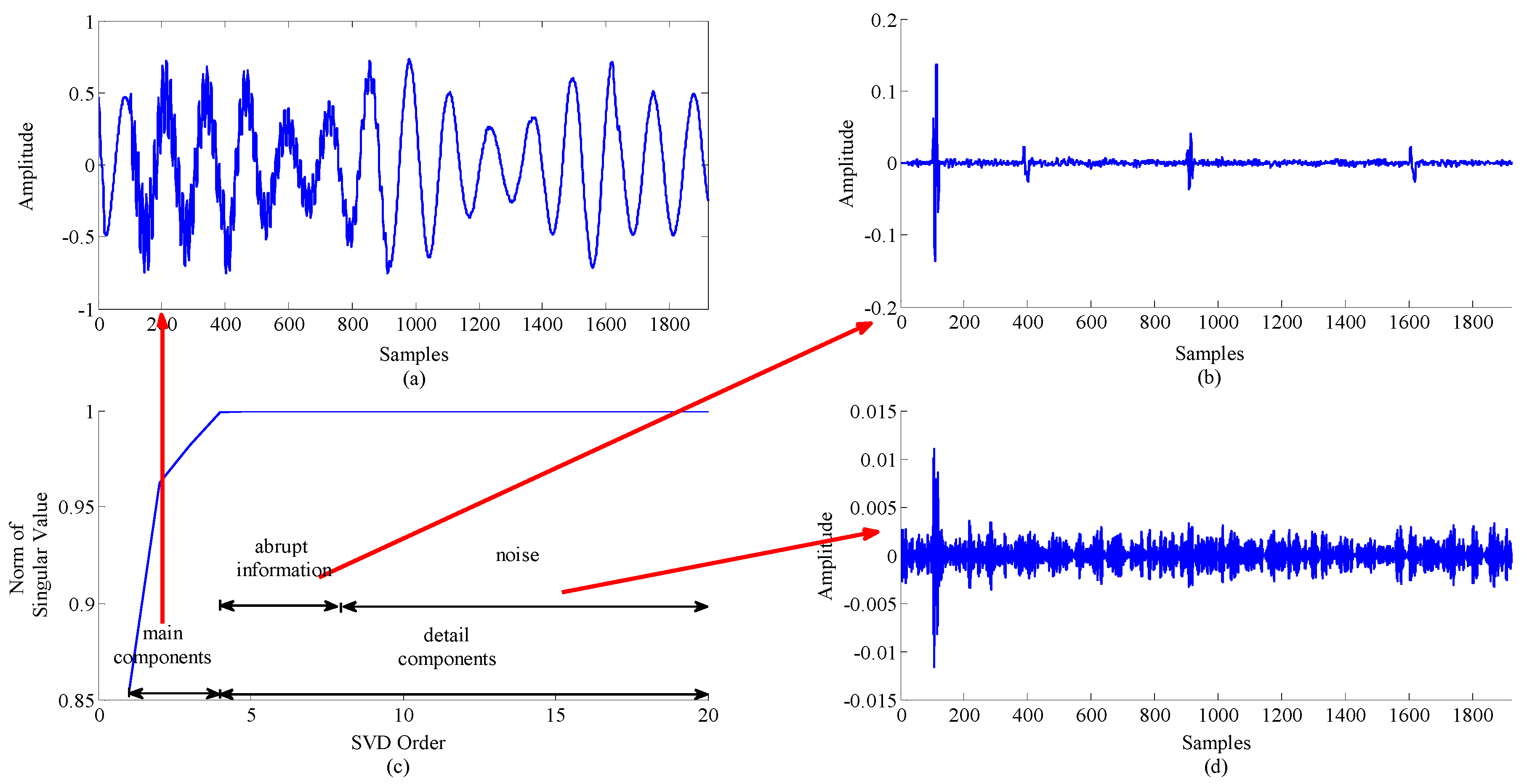
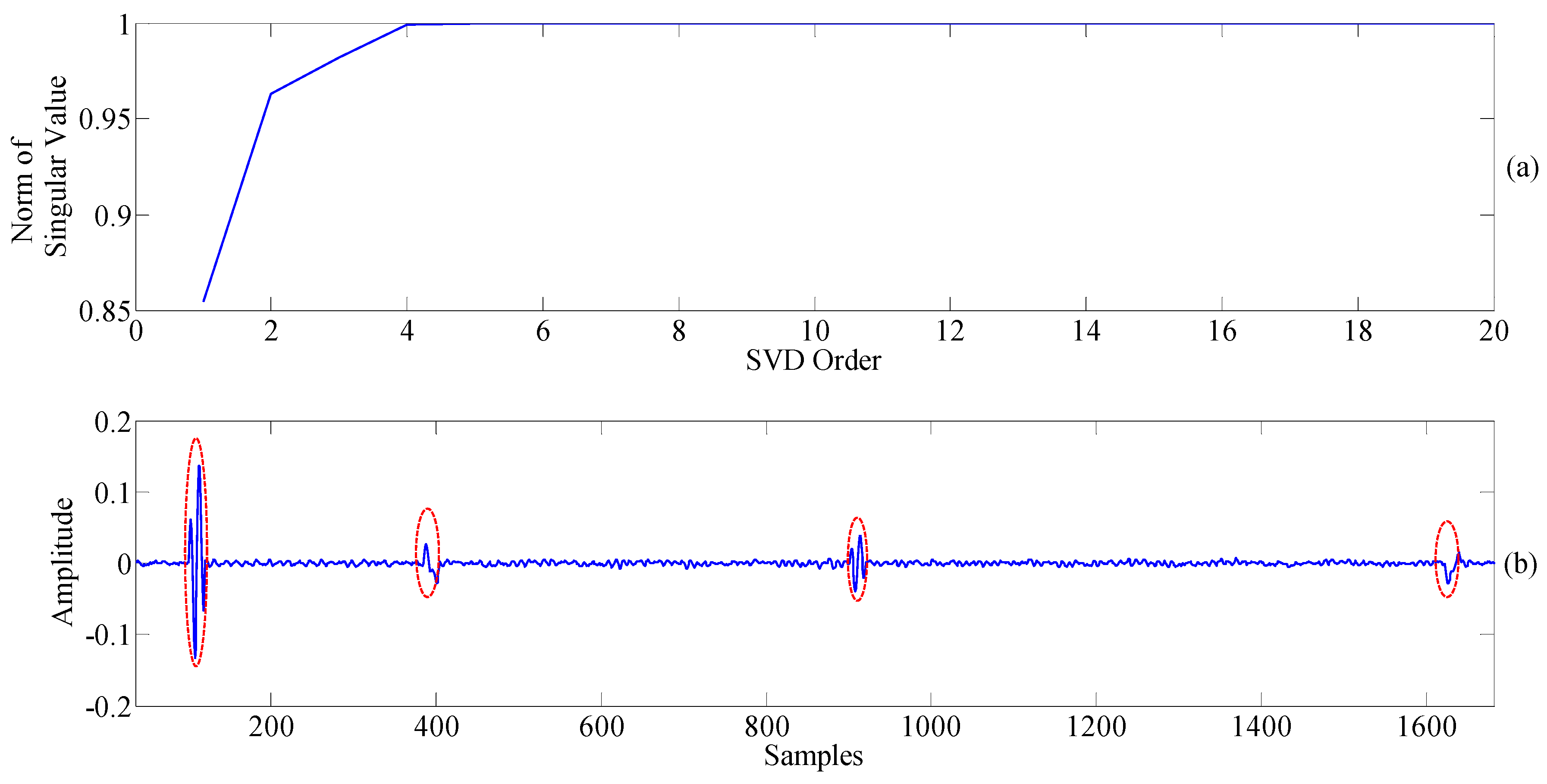
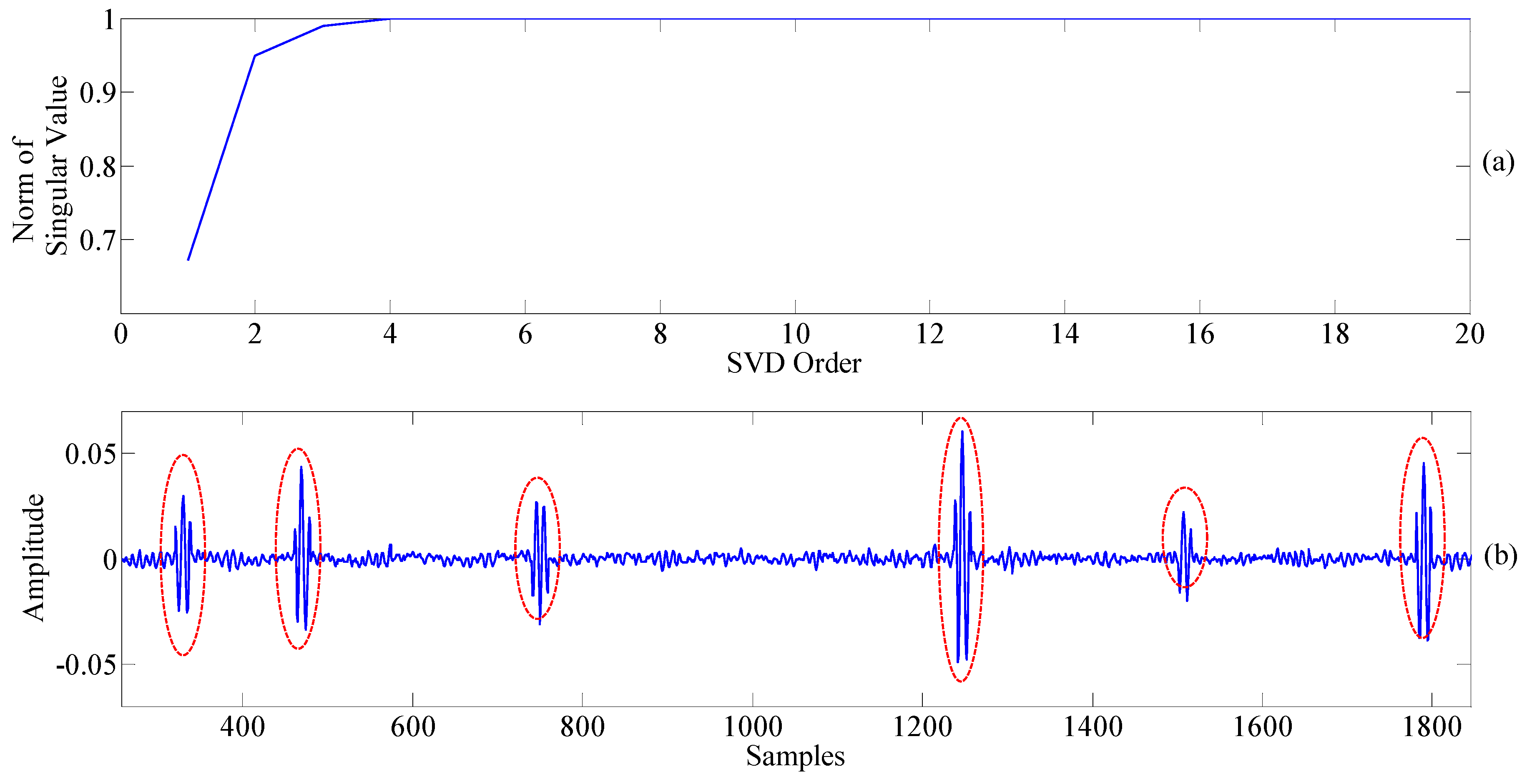
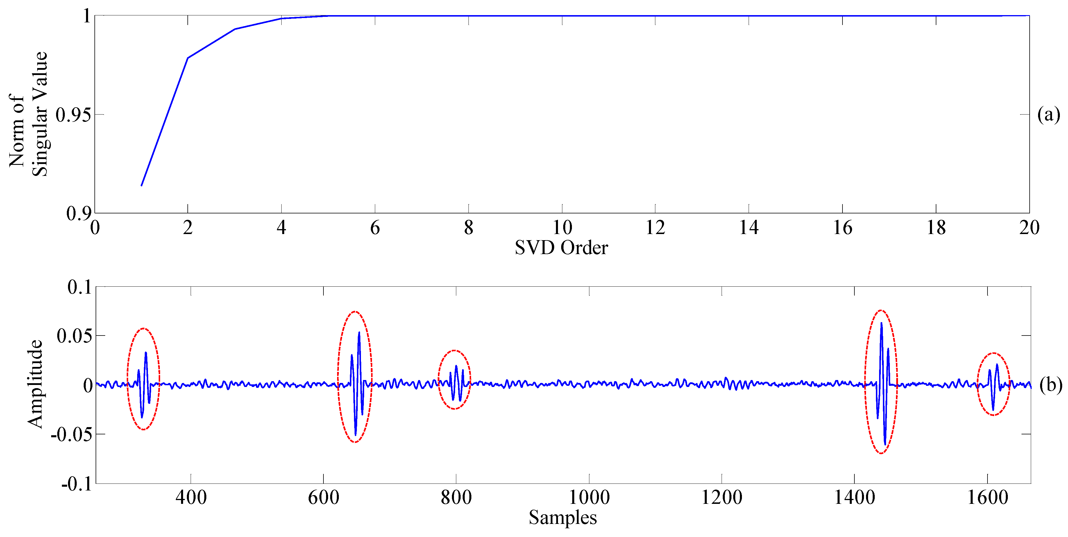
As TLS-ESPRIT is not good at identifying time-varying sequences, an abrupt information extraction method based on the singular value decomposition of signal’s Hankel matrix is proposed in this paper. A hierarchical method of abrupt information layer based on singular value norm is also proposed. According to the catastrophe points identified by this method, the original time-varying signal can be accurately divided into several intervals with stationary characteristics, and the starting and ending time of PQ events are precisely located.

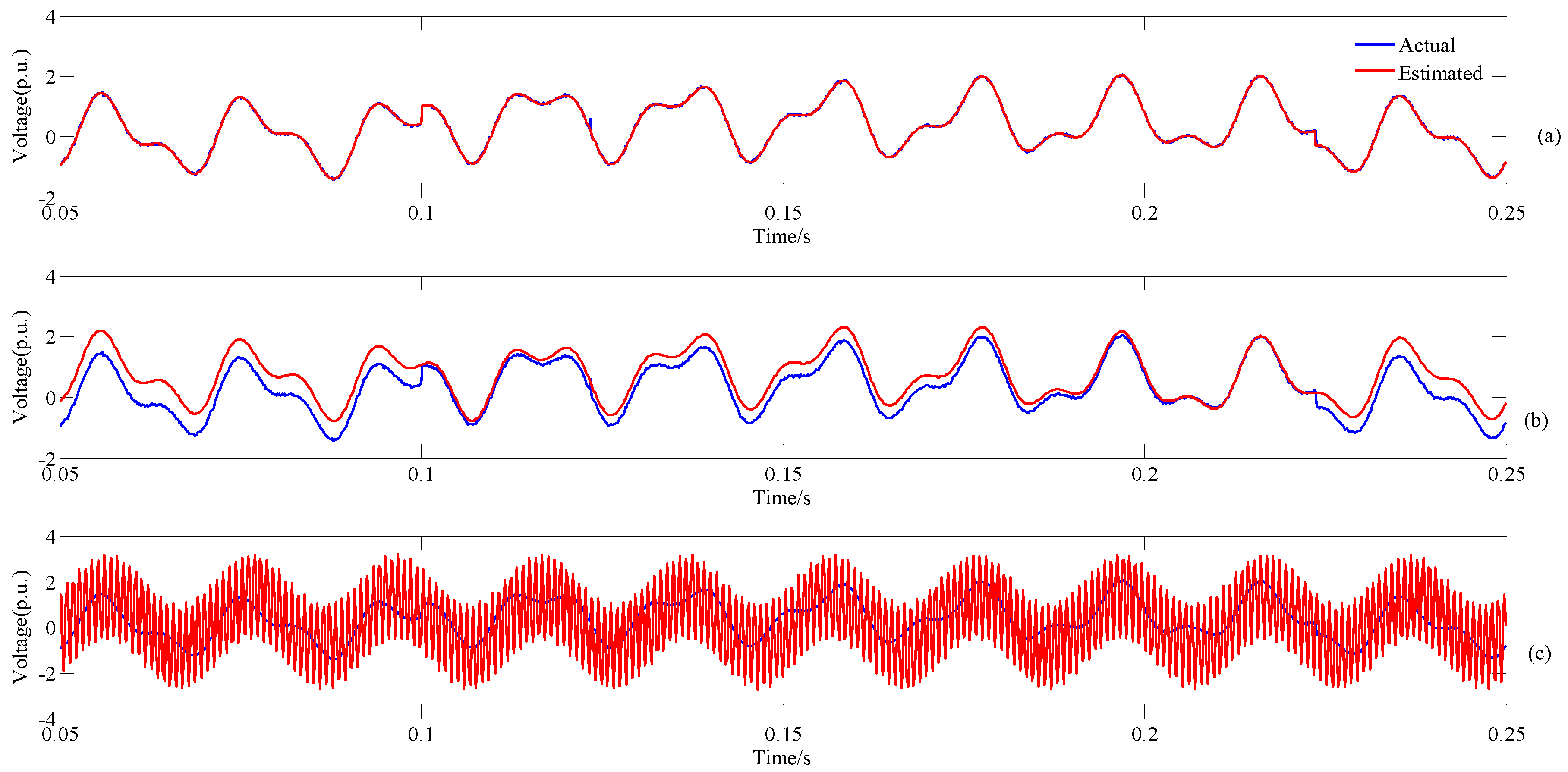
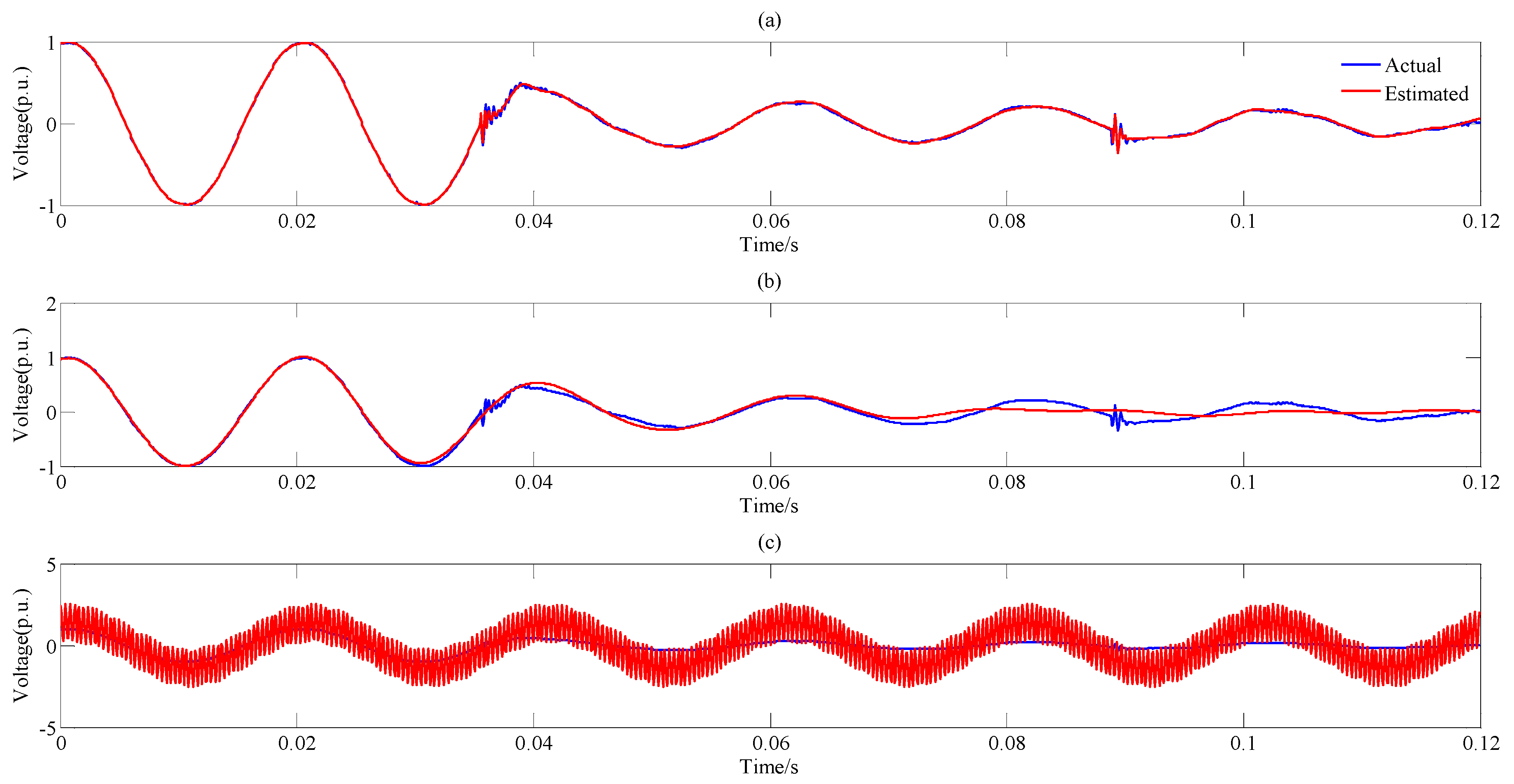
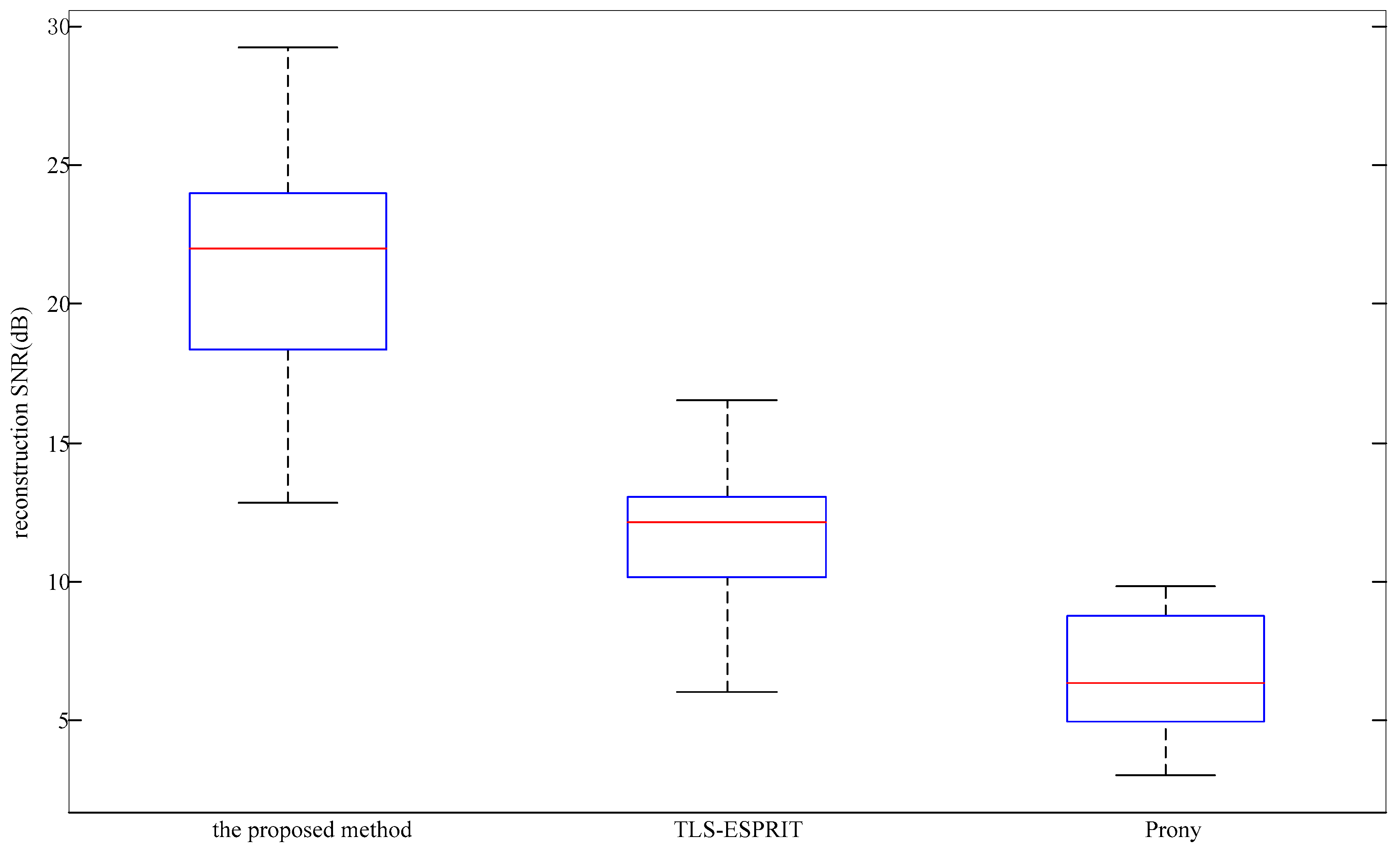
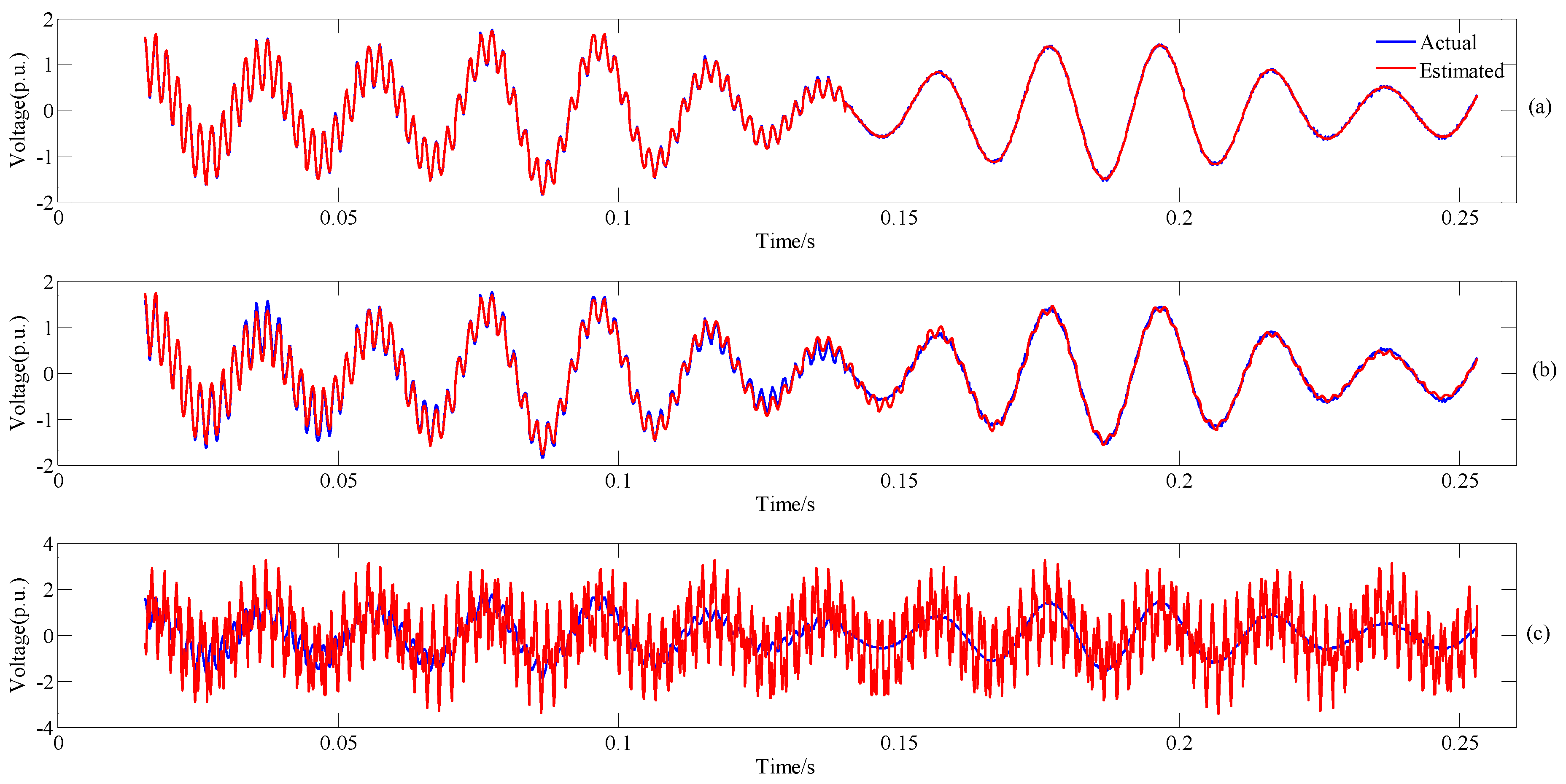
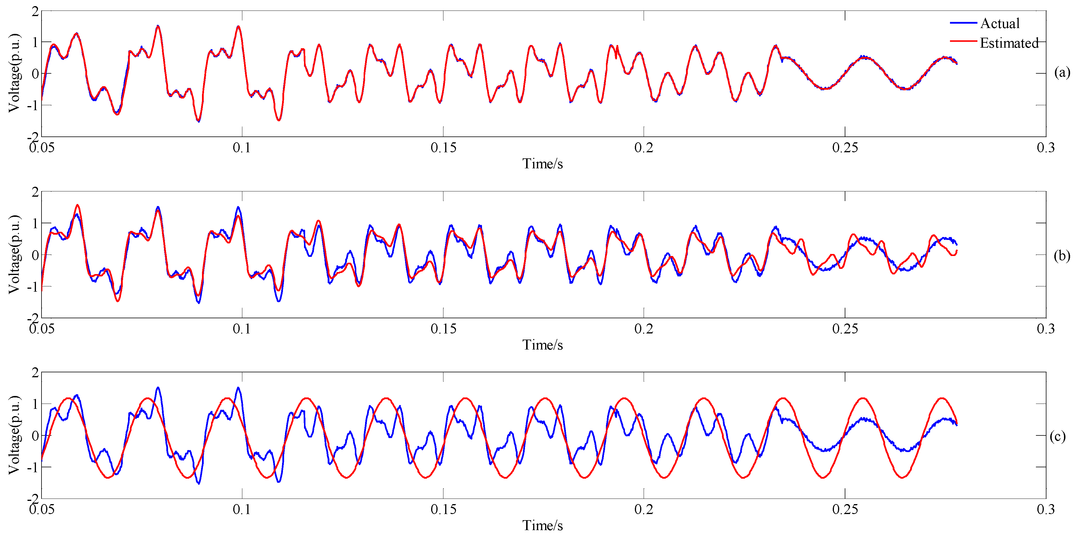
An improved TLS-ESPRIT method based on the sectional treatment and singular value norm is proposed, which has a higher accuracy of combined disturbance identification than traditional method, and its practicality is also verified by the IEEE PES DATABASE measured signals and real-world data.

In addition, the matrix operation in TLS-ESPRIT in this paper is less time consuming because of the subsection processing technology, and the disturbance locating method based on SVD has a low computational complexity. Thus, the efficiency of disturbance identification is greatly improved.

The accurate locating of the disturbance and the accurate identification of the parameters are helpful to reveal the complete process and comprehensive information of the complex disturbance events. They also have important guiding value in analyzing the consequences, finding out the accountability of the incident and controlling power quality pollution, which will be the next step of this research direction.

References

1. Borrás, M.D.; Bravo, J.C.; Montaño, J.C. Disturbance ratio for optimal multi-event classification in power distribution networks. IEEE Trans. Ind. Electron. 2016, 63, 3117–3127. [Google Scholar] [CrossRef]
2. Ribeiro, M.V.; Pereira, J.L.R. Classification of single and multiple disturbances in electric signals. EURASIP J. Adv. Signal Process. 2007, 2007, 15. [Google Scholar] [CrossRef]
3. Kumar, R.; Singh, B.; Shahani, D.T. Symmetrical components-based modified technique for power-quality disturbances detection and classification. IEEE Trans. Ind. Appl. 2016, 52, 3443–3450. [Google Scholar] [CrossRef]
4. Shukla, S.; Mishra, S.; Singh, B. Power quality event classification under noisy conditions using EMD-based de-noising techniques. IEEE Trans. Ind. Inform. 2014, 10, 1044–1054. [Google Scholar] [CrossRef]
5. Azam, M.S.; Tu, F.; Pattipati, K.R.; Karanam, R. A dependency model-based approach for identifying and evaluating power quality problems. IEEE Trans. Power Deliv. 2004, 19, 1154–1166. [Google Scholar] [CrossRef]
6. De Yong, D.; Bhowmik, S.; Magnago, F. An effective power quality classifier using wavelet transform and support vector machines. Expert Syst. Appl. 2015, 42, 6075–6081. [Google Scholar] [CrossRef]
7. Bhende, C.N.; Mishra, S.; Panigrahi, B.K. Detection and classification of power quality disturbances using S-transform and modular neural network. Electr. Power Syst. Res. 2008, 78, 122–128. [Google Scholar] [CrossRef]
8. Kumar, R.; Singh, B.; Shahani, D.T.; Chandra, A.; Al-Haddad, K. Recognition of power-quality disturbances using S-transform-based ANN classifier and rule-based decision tree. IEEE Trans. Ind. Appl. 2015, 51, 1249–1257. [Google Scholar] [CrossRef]
9. Liu, Z.; Cui, Y.; Li, W. A classification method for complex power quality disturbances using EEMD and rank wavelet SVM. IEEE Trans. Smart Grid 2015, 6, 1678–1685. [Google Scholar] [CrossRef]
10. Fengzhan, Z.; Rengang, Y. Power quality disturbance recognition using S-transform. IEEE Trans. Power Deliv. 2007, 22, 944–950. [Google Scholar]
11. Ibrahim, W.R.A.; Morcos, M.M. A power quality perspective to system operational diagnosis using fuzzy logic and adaptive techniques. IEEE Trans. Power Deliv. 2003, 18, 903–909. [Google Scholar] [CrossRef]
12. Wen, H.; Guo, S.; Teng, Z.; Li, F.; Yang, Y. Frequency estimation of distorted and noisy signals in power systems by FFT-based approach. IEEE Trans. Power Syst. 2014, 29, 765–774. [Google Scholar] [CrossRef]
13. Wright, P.S. Short-time Fourier transforms and Wigner–Ville distributions applied to the calibration of power frequency harmonic analyzers. IEEE Trans. Instrum. Meas. 1999, 48, 475–478. [Google Scholar] [CrossRef]
14. Tse, N.C.F.; Chan, J.Y.C.; Lau, W.-H.; Lai, L.L. Hybrid wavelet and Hilbert transform with frequency-shifting decomposition for power quality analysis. IEEE Trans. Instrum. Meas. 2012, 61, 3225–3233. [Google Scholar] [CrossRef]
15. Afroni, M.J.; Sutanto, D.; Stirling, D. Analysis of non-stationary power quality waveforms using iterative Hilbert huang transform and SAX algorithms. IEEE Trans. Power Deliv. 2013, 28, 2134–2144. [Google Scholar] [CrossRef]
16. De la O Serna, J.A. Synchrophasor estimation using Prony’s method. IEEE Trans. Instrum. Meas. 2013, 62, 2119–2128. [Google Scholar] [CrossRef]
17. Sheshyekani, K.; Fallahi, G.; Hamzeh, M.; Kheradmandi, M. A general noise-resilient technique based on the matrix pencil method for the assessment of harmonics and interharmonics in power systems. IEEE Trans. Power Deliv. 2017, 32, 2179–2188. [Google Scholar] [CrossRef]
18. Reddy, J.; Dash, P.K.; Samantaray, R.; Moharana, A.K. Fast tracking of power quality disturbance signals using an optimized unscented filter. IEEE Trans. Instrum. Meas. 2009, 58, 3493–3952. [Google Scholar] [CrossRef]
19. Manikandan, M.S.; Samantaray, S.R.; Kamwa, I. Detection and classification of power quality disturbances using sparse signal decomposition on hybrid dictionaries. IEEE Trans. Instrum. Meas. 2015, 64, 27–38. [Google Scholar] [CrossRef]
20. Song, H.; Huang, C.; Liu, H.; Chen, T.J.; Li, J.L.; Luo, Y. A new power quality disturbance detection method based on the improved LMD. Proc. CSEE 2014, 34, 1700–1708. [Google Scholar]
21. Valtierra-Rodriguez, M.; Romero-Troncoso, R.D.J.; Osornio-Rios, R.A.; Garcia-Perez, A. Detection and classification of single and combined power quality disturbances using neural networks. IEEE Trans. Ind. Electron. 2014, 61, 2473–2482. [Google Scholar] [CrossRef]
22. Laila, D.S.; Messina, A.R.; Pal, B.C. A refined Hilbert-Huang transform with applications to inter-area oscillation monitoring. IEEE Trans. Power Syst. 2009, 24, 610–619. [Google Scholar] [CrossRef] [Green Version]
23. Huang, N.E.; Shen, Z.; Long, S.R.; Wu, M.C.; Shih, H.H.; Zheng, Q.; Yen, N.; Tung, C.C.; Liu, H.H. The empirical mode decomposition and the Hilbert spectrum for nonlinear and non-stationary time series analysis. Proc. R. Soc. Lond. Ser. A Math. Phys. Eng. Sci. 1998, 454, 903–995. [Google Scholar] [CrossRef]
24. Borges, F.; Fernandes, R.; Silva, I.; Silva, C.B.S. Feature extraction and power quality disturbances classification using smart meters. IEEE Trans. Ind. Inform. 2016, 12, 824–833. [Google Scholar] [CrossRef]
25. Roy, R.; Kailath, T. ESPRIT-estimation of signal parameters via rotational invariance techniques. IEEE Trans. Acoust. Speech Signal Process. 1989, 37, 984–995. [Google Scholar] [CrossRef]
26. Landesa, L.; Obelleiro, F. Bias of the maximum likelihood DOA estimation from inaccurate knowledge of the antenna array response. J. Electromagn. Waves Appl. 2007, 21, 1205–1217. [Google Scholar]
27. Xiao, J.; Xie, X.; Han, Y.; Wu, J. Dynamic tracking of low-frequency oscillations with improved prony method in wide-area measurement system. In Proceedings of the 2014 IEEE Power Engineering Society General Meeting, Denver, CO, USA, 6–10 June 2004. [Google Scholar]
28. Hua, Y.; Sarkar, T.K. Matrix pencil method for estimating parameters of exponentially damped/undamped sinusoids in noise. IEEE Trans. Acoust. Speech Signal Process. 1990, 38, 814–824. [Google Scholar] [CrossRef]
29. Zhao, X.; Ye, B.; Chen, T. Influence of matrix creation way on signal processing effect of singular value decomposition. J. South China Univ. Technol. (Nat. Sci. Ed.) 2008, 36, 86–93. [Google Scholar]
30. Smith, J.C.; Hensley, G.; Ray, L.; Andresen, M.; Thomas, K.; Roberts, J.; Basch, V.; King, J.; St. John, A.; Bergeron, R.; et al. IEEE Standard 1159–2009: IEEE Recommended Practice for Monitoring Electric Power Quality; IEEE: Piscataway, NJ, USA, June 2009. [Google Scholar]
31. IEEE Power Engineering Society. IEEE PES Working Group P1433 Power Quality Definitions. Available online: http://grouper.ieee.org/groups/1159/2/testwave.html (accessed on 2 February 2001).
Figure 1. The reconstruction SNR and relative error of parameters with different sampling frequency and number of cycles: (a) The relative error of amplitude; (b) The relative error of frequency; (c) The relative error of initial phase; (d) The relative error of damping ratio; (e) SNRrec of the test signal.
Energies 10 01809 g001
Figure 2. (a) Norm of singular value with different l; (b) The er of 50 Hz component with l increasing; (c) The er of 150 Hz component with l increasing.
Energies 10 01809 g002
Figure 3. The schematic diagram of catastrophe points location. (a) The main components; (b) The abrupt information; (c) The norm of singular value; (d) The noise.
Energies 10 01809 g003
Figure 4. The flowchart for measurement of power quality.
Energies 10 01809 g004
Figure 5. Detection of catastrophe points in signal described by Equation (18). (a) Norm of singular value; (b) The waveform of P5.
Energies 10 01809 g005
Figure 6. Source signal and the reconstruction of (25) by using (a) The proposed method; (b) TLS-ESPRIT; (c) Prony method.
Energies 10 01809 g006
Figure 7. Detection of catastrophe points in signal described by Equation (20). (a) Norm of singular value; (b) The waveform of P5.
Energies 10 01809 g007
Figure 8. Source signal and the reconstruction of Equation (20) by using (a) The proposed method; (b) TLS-ESPRIT; (c) Prony method.
Energies 10 01809 g008
Figure 9. Detection of catastrophe points in signal described by Equation (21). (a) Norm of singular value; (b) The waveform of P5.
Energies 10 01809 g009
Figure 10. Detection of pulse.
Energies 10 01809 g010
Figure 11. Source signal and the reconstruction of Equation (21) by using (a) The proposed method; (b) TLS-ESPRIT; (c) Prony method.
Energies 10 01809 g011
Figure 12. Source signal from IEEE PES Database and the reconstruction by using (a) The proposed method; (b) TLS-ESPRIT; (c) Prony method.
Energies 10 01809 g012
Figure 13. The SNRrec with different methods.
Energies 10 01809 g013