Metaheuristic Techniques in Enhancing the Efficiency and Performance of Thermo-Electric Cooling Devices

Abstract

The objective of this paper is to focus on the technical issues of single-stage thermo-electric coolers (TECs) and two-stage TECs and then apply new methods in optimizing the dimensions of TECs. In detail, some metaheuristics—simulated annealing (SA) and differential evolution (DE)—are applied to search the optimal design parameters of both types of TEC, which yielded cooling rates and coefficients of performance (COPs) individually and simultaneously. The optimization findings obtained by using SA and DE are validated by applying them in some defined test cases taking into consideration non-linear inequality and non-linear equality constraint conditions. The performance of SA and DE are verified after comparing the findings with the ones obtained applying the genetic algorithm (GA) and hybridization technique (HSAGA and HSADE). Mathematical modelling and parameter setting of TEC is combined with SA and DE to find better optimal findings. The work revealed that SA and DE can be applied successfully to solve single-objective and multi-objective TEC optimization problems. In terms of stability, reliability, robustness and computational efficiency, they provide better performance than GA. Multi-objective optimizations considering both objective functions are useful for the designer to find the suitable design parameters of TECs which balance the important roles of cooling rate and COP.

1. Introduction

The Mud-Pulse High-Temperature (MWD) is known as a system used for performing drilling- related measurements down-hole and transmitting information to the surface while drilling a well [1]. A typical High Temperature MWD tool structure is presented in Figure 1.

A MWD is able to use some measurements such as tool face, natural gamma rays, borehole pressure, directional survey, vibration, temperature, torque, and shock. Achieving optimal payload temperatures in down-hole environment at 230 °C needs a MWD cooling system that can pump a remarkable load and also a low thermal resistance path on the heat rejection (hot side). At this point, high temperature thermo-electric cooler (TEC) materials and assemblies should be employed for such an application environment with high pressure, high temperature, mechanical shock and vibration requirements. In order to obtain optimal operating conditions in the MWD, electronic-cooling components located in MWD housing are very important. This can be achieved thanks to thermo-electric cooling devices with thin-film forms. Figure 2 shows the position of a TEC in the thermal management system of MWD device.

A TEC is a solid-state cooling device that uses the Peltier effect over p-type and n-type semiconductor elements, unlike refrigerators, which are vapor-cycle based [3]. TECs are employed for converting the electrical energy into a temperature gradient. A TEC does not use any refrigerant or moving parts, which make these devices highly reliable and also require low maintenance. Furthermore, a TEC does not generate noise (both electrical and acoustical) and is known as ecologically clean. Considering its weight and size, a TEC is lightweight and also has a compact size. It is also important that TECs have high precision in controlling the temperature. On the other hand, another remarkable TEC feature that should be mentioned is that it has the capacity for use in cooling instruments (like a MWD) in the case of extreme physical conditions. TECs come in two types: single-stage or multi-stage. Figure 3 shows thermo-electric coolers of the single-stage and two-stage type, respectively.

The single-stage TEC (STEC), which is commercially available and shown in Figure 3a can provide a temperature difference of about 60–70 °K at maximum in the case the hot side is at room temperature [3], but when it is needed to have a large temperature difference in some applications, a STEC will not be able to do that. At this point, in order to solve this issue of TECs, an alternative type of TEC, called two-stage TEC (TTEC, shown in Figure 3b) or a multi-stages TEC is employed [4]. For enhancing the transfer of heat and also general system performance, the thermo-electric module here works with two heat sinks located over both its hot and cold sides.

Generally, the application scope of TECs is limited by their ability to dissipate only a limited amount of heat flux and relatively low energy conversion efficiency. At this point, two parameters—maximum cooling rate and maximum coefficient of performance (COP)—have a great role on the focus point of the TEC. A TEC typically runs at about 5–10% of Carnot cycle COP while compressor- based refrigerators runs at more than 30% as default. Here, it could be good to use engineering design optimization for TECs, and metaheuristics, which are intelligent optimization techniques, can be used for that engineering design optimization [5]. Until now, Genetic Algorithm (GA) [6] and the extended version of GA which is Non-dominated Sorting Genetic Algorithm (NSGA-II) [7,8] are two metaheuristic optimization techniques that were employed in optimizing the performance of both types of TEC. However, their behavior and search capability have not analyzed deeply or the performed researches with GA and NSGA-II have some disadvantages (these are explained in detail in Section 2.3 in the following pages).

1.1. Problem Statement

Use of a TEC as a cooling solution for instruments located in extreme environments (especially in thermal energy and gas drilling operations) is a very important application, but because of some drawbacks like relatively low energy conversion efficiency and the ability to dissipate only a limited amount of heat flux, the performance and efficiency of these devices can be affected negatively.

Considering the past literature, it is possible to indicate that performance evaluation of the meta-heuristic like GA and NSGA-II within TEC is limited and comes with poor analysis results, so, it is critical to perform more investigation and detailed analysis by using some defined criteria such as measuring the convergence speed, stability, reliability, robustness, computational efficiency.

In the past, some meta-heuristic techniques like Simulated Annealing (SA) [9,10,11], and some other evolutionary algorithms (GA [6], Differential Evolution (DE) [12,13,14]) were used in their pure and hybridized forms to improve the effectiveness of the optimization process regarding TEC model, benefitting from a large number of variables (physical, as well as geometrical properties), and also obtain more performance in the objective problem. GA has been applied firstly to improve the benefits of TEC, but has difficulties in parameter selection. SA and DE have not been applied for TEC but has been proven with advantages when applied in optimizing thermal energy systems.

1.2. Objectives and Motivations of the Study

DE belongs to the same family as GA but has been claimed to have better performance than GA in many applications. SA has the capability to escape from local optima better than GA while trying to obtain global optimality (these advantages of DE and SA are discussed briefly with literature references in Sub-Section 2.4 in the following pages). Therefore, in this research, the objectives are:

▪

To investigate using metaheuristic stand-alone techniques like SA and DE for STEC and TTEC.

▪

To develop hybrid techniques for STEC and TTEC.

▪

To validate the all the techniques (stand-alone and hybrid) on STEC and TTEC.

This research mainly focuses on simulation studies of the system. Metaheuristics, which are SA, DE and suggested hybridized techniques are combined with the STEC and TTEC model and put on an integrated MATLAB platform (2013a, MathWorks, Natick, MA, USA). In that system, objectives are cooling rate and COP. They are optimized individually or simultaneously using single-objective optimization or multi-objective optimization approaches, respectively. The design variables and their boundaries, constraints and other fixed parameters need to be identified. The performance of each technique is evaluated based on simulation findings. The comparative study of the computational findings between metaheuristic algorithms−techniques with references of previous works is also studied to propose the best performance technique.

The research here contributes to the associated literature by employing some remarkable optimization algorithms, which are SA, DE and also hybridized techniques, to enhance the efficiency of TECs by finding optimal design parameters. Most of the research work in improving the TECs’ performance focuses on optimizing the material properties of the TEC, but the material properties are restricted by technological limitations and the fabrication processes. Until now, there is a limited number of optimization techniques, especially the GA is the only metaheuristic that has been applied in optimizing the design parameters of TECs. By using some other optimization techniques in metaheuristics with better search ability and capability of handling a diversity of TECs’ problems, the improvement of efficiency and performance of TECs can be better achieved.

The most important contribution is a systematic approach to perform testing and evaluation of the metaheuristics. In previous research, the performance of optimization methods like GA was evaluated by a few criteria such as convergence analysis and a discussion of the comparison with analytical findings (That is discussed more within the next pages). By applying more test types like stability and reliability analysis, computational efficiency and robustness measurement, the behavior of each metaheuristic can be investigated in depth and compared.

Considering the subject and objectives—motivations of the study, the rest of the paper is organized as follows: the next section explains the basic structure and operational principle of the TEC module. Metaheuristic techniques, which are SA, DE and GA, are also presented with a comparison of their benefits. Then, related works that have been applied to optimization issues of the design parameters and material properties of TECs including STECs and TTECs are reviewed. A critical analysis section is built to discuss the weaknesses of previous research and synthesize the needed information that is included in this research. Following to that, the third section presents the research methodology of our study. Firstly, mathematical modelling of STECs and TTECs are introduced. The relation between two main parameters which are cooling rate and COP, together with the impact of geometric properties and material properties are reported. Secondly, single-objective optimization and multi-objective optimization approach with respect objective functions, taking into account all related parameters are presented. Next, SA, DE and the suggested hybridized techniques HSAGA, HSADE are described in detail with the flowchart of the algorithms and parameter settings. The research issues which include the testing procedure criteria to evaluate all the algorithms are presented. After the third section, section four focuses on the tests related to SA and DE techniques. By applying mathematical modelling of TECs and the operation procedure of the algorithms in MATLAB, the behaviors of the algorithms are evaluated scientifically. Parameter selection of the TEC model and the algorithms are also reported with the related references and settings from prior experiences. After the evaluations of the algorithm are stated based on recommended criteria, the section also presents some case studies which yield some new optimal findings considering single-objective optimization and multi-objective optimization for both types of TEC. In addition, the best TEC designs balancing between cooling and COP and satisfying the constraint conditions are reported. After all these sections, the fifth section provides a general discussion and the paper ends in the last section with explanations on the conclusions and some future works.

2. Background

This section reviews basic knowledge of TEC devices such as their structure and thermo-electric effects. The metaheuristic techniques are also reviewed, including three different techniques chosen according to their essential differences such as point-based, population-based and hybridization- oriented. Related works that have been applied in optimizing the performance of TECs, analysis and discussion along the line of the problem, the issues and challenges are also reviewed in this section.

2.1. Basic Structure and Operation Principle of TEC

A TEC is briefly formed by thermo-electric couples, which are n-type and also p-type semiconductor elements. Thermo-electric couples are connected in series electrically, in parallel thermally, and finally fixed by soldering, located between two ceramic plates. The latter form the hold and cold TEC sides [15]. A STEC module employs a pair of cold and warm sides, and one matrix of pellets. A TTEC or multi-stage module can be seen as a structure of two or more single stages, which are stacked on top of each other. As general, a TTEC or multi-stage module is constructed as a pyramidal type, each lower stage is bigger than the upper stage. In detail, once the top stage is employed for cooling, the lower stage needs greater cooling capacity to pump heat, which is dissipated from the upper stage [16].

The thermo-electric effect can be described as the conversion of energy between electricity and heat. There are three types of thermo-electric effects that occur. These effects are called as Seebeck, Peltier, and Thomson, respectively [17]. These effects are found to be thermodynamically reversible and act in combination with irreversible effects such as Joule heating and thermal conduction.

▪

Seebeck Effect: If A and B: two dissimilar semiconductors are joined at two points and the temperature difference ΔT is maintained between the two junctions, then an open-circuit potential difference ΔV will be developed. This is called the Seebeck effect. The equation is presented in Equation (1) defines the differential Seebeck coefficient α between two dissimilar conductors:

$${\alpha }_{AB}=\underset{\Delta T\to 0}{\lim }\frac{\Delta V}{\Delta T}\left(V/{}^{o}K\right)$$

(1)

For small ΔT, a linear relation occurs. If the coefficient of Seebeck is known, the temperature difference can be measured through measuring Seebeck voltage. The sign regarding α_AB is positive when the ΔV causes a current to flow in a clockwise direction as around the circuit.

▪

Peltier Effect: Peltier is briefly the principal effect concerned with thermo-electric refrigeration of heat pumping. At the time A and B: two different conductors are joined together and electric current flows through the one direction, heat will be generated or absorbed at the junction at a constant rate. The Peltier coefficient is determined based on Equation (2):

$${\pi }_{AB}=\frac{Q}{I}$$

(2)

Q is known as Peltier heat or heat generation. The rate at which heat is absorbed is proportional to the current and associated with the nature of the two materials, which comprises the junction. Comparing with the Seebeck effect, where heat flow induces an electric current, the Peltier effect is opposite, with an electric current induced a heating or cooling effect. These two thermo-electric effects are thermodynamically related by means of so-called Kelvin relation as shown in Equation (3):

$$\pi =\alpha \times T$$

(3)

▪

Thomson Effect: As the last of the thermo-electric effects, the Thomson effect is associated with the rate of generation of reversible heat Q resulting from the passage of a current along a portion of a single conductor along which there is a ΔT. The Thomson effect is not of primary importance in thermo-electric device but it should not be neglected in detailed calculations.

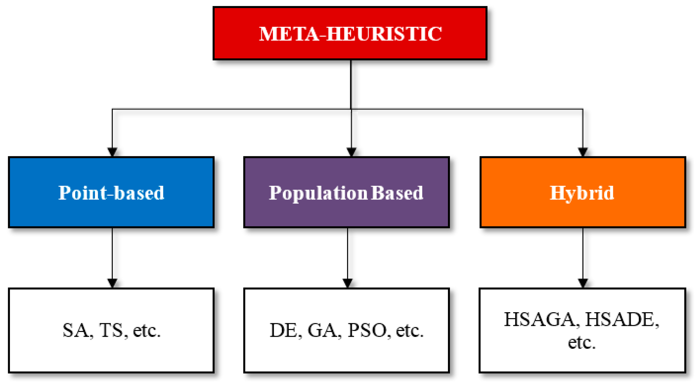
2.2. Metaheuristic Optimization Algorithms

For a long time, metaheuristics have been known as effective and efficient approaches for many hard to solve optimization problems [18]. Briefly, a metaheuristic is an algorithm for solving optimization problems (especially hard ones) without being deeply adapted to the objective problem [19]. From a general perspective, almost all meta-heuristics employ the characteristic of being nature-inspired (based on some principles from physic, biology or ethnology) [20]. Typical categories of metaheuristic algorithms are shown in Figure 4.

There are three types of metaheuristics technique can be described as follows:

▪

Point-based: Point-based methods focus on a single solution at the start and then moves away from it, drawing a trajectory within the search space [21]. Some algorithms like SA (Simulated Annealing), and TS (Tabu Search) are popular point-based metaheuristic techniques.

▪

Population-based: Population-based methods focused on a set (or similarly called group) of solutions rather than just a single solution [22]. Some of the most popular population-based methods are GA (Genetic Algorithms), DE (Differential Evolution) and PSO (Particle Swarm Optimization).

▪

Hybrid optimization: Hybrid optimization methods are one of the most interesting research trends nowadays. Hybridized algorithms are not just the combination of different point-based or population-based metaheuristics [23]. The combination can benefit from the advantages and strengths of each employed algorithm so as to improve algorithm performance, overcome the individual weaknesses and be more effective and efficient during problem-solving processes [24].

It is important for a metaheuristic to have a balance between the exploration and exploitation in order to be successful in the objective optimization problem [25]. At this point, basic point-based metaheuristic techniques are more exploitation-oriented while the population-based ones are more exploration-oriented. Here, an exploration (diversification) process is necessary for detecting the related parts of the search space having high quality solutions. On the other hand, exploitation (intensification) is also necessary to direct the searching to some promising areas of the accumulated search experience [25]. Moving from that, it is possible to indicate that differences among existing metaheuristics is associated with the way, which they use to achieve this balance.

2.3. Literature Review

Here, the known disadvantages of TEC such as the poor COP and also low cooling rate are discussed. These factors can be updated (improved) separately or simultaneously. The parameters in the cooling rate and COP equations can be examined under three different categories: specifications, material properties, and design parameters [17]:

▪

Operating temperature T_c and T_h, the needed output voltage V, current I, and power output P are known as the specifications. These are usually provided by customers according to requirements within a specific application.

▪

The material parameters are based on the status of current materials and the technologies regarding module fabrication. As a result of the effect of material properties on TEC performance, many research works were realized during the past ten years in order to find new materials and structures for use in a green system with highly efficient cooling and also energy conversion. With the highest value figure of merit (ZT), bismuth-telluride (Bi₂Te₃) is among the best thermo-electric materials [26]. By doping or alloying some other elements in several fabrication processes, there has been a remarkable effort to raise the ZT of bulk materials based on Bi₂Te₃. At the end, it has been seen that the ZT value was not much more than one and seems insufficient to improve the cooling efficiency. That is because of the difficulty of increasing the electrical conductivity or Seeback coefficient without realizing a corresponding increase in the thermal conductivity [27]. The work by Poudel et al. describes recent advances in improving ZT values [28]. They have achieved a peak ZT of 1.4 at 100 °C suing a bismuth antimony telluride (BiSbTe) p-type nanocrystalline bulk alloy. This material is an alloy of Bi₂Te₃ and generally obtained by hot pressing nanopowders, which are ball-milled from crystalline ingots. These materials are useful for microprocessor cooling applications because ZT is about 1.2 at room temperature and peaks at about 1.4 at 100 °C.

▪

Eventually, TEC design aims to determine a set of design parameters appropriate for the necessary specifications or effective on achieving the best performance at aminimum cost.

Table 1. Details regarding optimization techniques used for the optimization of TEC.

Author	Application	Advantages and Disadvantages
Cheng [29]	GA is applied to optimize the geometric design of STECs	GA proves fast convergence speed and effective search, but GA parameter setting is not suggested or discussed.
Cheng [30]	GA is applied to optimize the design parameter of TTECs	GA was applied successfully to solve a heavier TTEC problem, but the robustness of GA when applied to for TTEC model is not very deterministic.
Huang [31]	Applies a conjugate-gradient method to optimize the geometric design of STECs	Effects regarding applied current and temperature on the optimum geometry are generally discussed. Performance analysis of the technique applied for STEC was not conducted. The base area of the studied STEC was small and not practical.
Nain [32]	Uses NSGA-II to optimize the geometric design of STECs	Multi-objective optimization is performed by optimizing cooling rate and COP simultaneously. Parameters of NSGA-II were chosen based on the authors’ experience, but the obtained findings are not reliable because of the unstable performance of the algorithm.
Rao [33]	Uses TLBO to optimize the design parameters of TTECs	Multi-objective optimization is performed. The performance of TLBO is evaluated and compared to GA, PSO by using some defined criteria, however, parameter selection for TLBO was not implemented.

lists details regarding the optimization techniques used in the optimization of TECs.

In single-objective optimization, Cheng et al. [29] were the first authors to use a metaheuristic which was GA to combine with a STEC model for finding optimal geometric designs. The geometric properties of semiconductor elements were accepted as the search variables and optimized simultaneously for reaching to the maximum cooling rate with also a few constraint conditions. Three case studies were performed under various applied current and various temperature differences ΔT to evaluate the effective search and create a better design data as compared to the designs available on the market. The GA algorithm was described and applied in the TEC model. However, there were many GA parameters such as total number of generations, crossover or mutation coefficient, etc. that needed to be defined. The authors did not suggest the parameters for the algorithm or describe a way to choose suitable values for every parameter. In another paper, these authors also employed the GA in order to maximize separately the cooling rate and COP but for a TTEC model [30]. In this research, two different types of TTEC which had different types of applied current were considered. Not the same as in geometric design of STECs, different types of TTEC design parameters were used as variables. They determined the current to the hot stage and cold stages of the TTEC, and the total number of semiconductor elements. Considering the effect of thermal resistance, the mathematical modeling of TTECs was heavier than for STECs [34]. The GA was applied successfully to solve the defined problems of TTECs, but the parameter selection of GA was not shown in this work. The authors claimed that GA had a robust behavior and effective search ability. However, the work is only based on the optimal design variables with respected maximum cooling rate and the comparison done is not enough to derive any ideas about the robustness of the algorithm.

Huang [31] introduced an optimization approach forming a complete multi-physics STEC model and a method of simplified conjugate-gradient, which is not a metaheuristic. Like in Cheng’s work, the geometric properties of the STEC were optimized as search variables in order to achieve the maximum cooling rate considering many operating conditions of temperature difference and applied current. In detail, effects of applied current and temperature difference over the optimal geometry were generally discussed. The authorscame up with a new better design than the initial one by using a conjugate-gradient method. However, the performance analysis of this technique applied to a STEC model was not done and the combined optimization is seen effective only for aminiature TEC with a base area of 9 mm², which is smaller than Cheng’s 100 mm² design [29] and not practical.

For multi-objective optimization, Nain [32,35] used an another version of GA which is Non-Dominated Sorting Genetic Algorithm II (NSGA-II) for solving the multi-objective optimization problems of STECs. The values of the geometric properties of a STEC were optimized to achieve Pareto-optimal solutions of cooling rate and COP values at different thermal resistance values. The benefits of obtaining the Pareto-frontier is the balance between cooling rate and COP, bringing benefits for the designer in choosing a suitable STEC design in practical application. However, the obtained findings are not reliable because there is a difference in the range of optimal design values between single-objective optimization and multi-objective optimization, caused by the instability of the algorithm. The parameters of the NSGA-II algorithm were chosen based on the authors’ experience, but they did not explain the selection method.

For TTECs, Rao [33] used modified teaching-learning-based optimization (TLBO) in optimizing the design parameters of two types of TTEC, like in Cheng’s work [30]. TLBO is inspired by a teacher’s influence over learners’ output in a class environment. TLBO was modified to increase its exploration and exploitation capacity. The modified TLBO was applied effectively to maximizing the cooling rate and COP of a TTEC simultaneously though having a heavy structure with twelve steps to finish a searching process. The determination of the total number of semiconductor elements as well as the supply current for both hot stage and cold stage were used as searching variables. This research has an improvement, namely that the ability of the TLBO and modified TLBO are compared to the GA and PSO approach by evaluating the convergence rate, the computational time and their obtained findings and by employing Sign and Wilcoxon statistical tests. However, parameter selection for TLBO and its modified version was not reported. The main importance parameters such as number of generations, population, teaching factor need to be indicated to clarify the selection of values used in optimizing TTEC.

2.4. Critical Analysis

In TEC, cooling rate is a main important value in considering the effectiveness of the TEC and is one main objective function in single-objective optimization or even multi-objective optimization. However, COP is also important and it’s a condition that needs to be satisfied in single-objective optimization and an objective in multi-objective optimization. Design parameters are also effective in determining the performance of a TEC. The impact of each design parameter is discussed. A well-selected design parameter can yield a significant cooling rate with a corresponding high COP. From the literature review, for STECs, the main design parameters are length, total number, and cross-sectional area of the semiconductor elements. For TTECs, the design parameters are total number of semiconductor elements in both TTEC stages and the applied current on the hot stage and cold stages.

Among metaheuristic techniques, GA is known as a population-based method, which is able to solve a constrained optimization problem and find excellent local optimization values [29]. GA could be successful on a variety of optimization problems thanks to the fact it searches a larger solution space [23], but it also needs determination of optimum controlling parameters like crossover rate and mutation rate, and also has a poor global search capability.

SA is known as a point-based metaheuristic. SA can escape from local optima [36], and has both flexibility and ability to achieve global optimality. Furthermore, SA can be used within large problems regardless of the conditions of differentiability, continuity, and convexity, as normally required in especially conventional optimization methods [37]. SA can also be easily coded even in complex systems and employed effectively in highly nonlinear model having many constraints. SA is generally an easy-to-understand metaheuristic and it is possible to code it easier than GA [38]. SA is robust against changes in the objective function, but GA should have the fitness function, which sometimes causes problems. SA seems also more readily useful for analysis processes. It was figured out that GA is too sensitive to the choice of mutation probability and fitness function while SA is too robust with regards to the choice of cooling schedule [39]. Also, findings—results obtained via GA—were disappointing especially in larger problem types.

DE is in the same family with GA. DE is considerably fast and robust technique for solving numerical optimization problems and has the capability to find global optima solutions [12]. DE has a more compact structure than GA with a simple computer code and has less control parameters. DE employ only three parameters as input to control the searching process, which is less than SA and GA. DE is currently among the most popular metaheuristics for solving single-objective optimization problems within continuous search spaces [20]. DE is generally a simple, and powerful algorithm that can outperform GA in many numerical single-objective optimization problems [40]. DE is able to explore the decision space more efficiently than GA even when multiple objectives need to be optimized [41]. From that premise, it is possible to indicate that the DE can also get better results than GA in numerical multi-objective optimization problems. However, DE has slow convergence speed for computationally expensive functions. By varying the control parameters the convergence speed of DE may increase, but it does not affect the quality of optimal solution.

Therefore, TEC performance can be enhanced by applying SA and DE intelligent algorithms into its mathematical modelling. Moreover, in most of the research papers about optimization of TECs, the effectiveness shown by the algorithm is evaluated over a few criteria such as convergence curve analysis, or by making a comparison with the optimal findings obtained by an analytical method and other optimization technique, or computational efficiency is discussed. The evaluation of the behavior of the metaheuristic like SA, DE and hybrid optimization technique needs to be performed strategically and more comprehensively based on the recommended testing criteria.

3. Methodology

This section discusses the mathematical modeling of STECs and TTECs. Cooling rate and COP equations are shown with the impact of relevant parameters such as geometric properties and material properties. Then, the research phases show the steps of how this research is implemented. Optimization algorithms of SA, DE and hybrid techniques are also described with their parameter settings.

3.1. Mathematical Modelling of STECs

A TEC is operated as based on the Peltier effect. The TEC briefly runs like a solid-state cooling device, which can pump heat from one junction to the other junction when a DC current is applied [29]. Energy balance equations over the hot junction and the cold junction for TEC can be indicated as in Equations (4) and (5). Q_c is the cooling rate that will be absorbed from the cooled side of TEC, Q_h is the heat rejection that will be released to the environment. The related equations point the completion between the Seebeck coefficient term associated with TEC cooling, and the parasitic effect regarding Joule heating and back heat conduction over the electrical resistance and thermal conductance terms, respectively. The heat flow αIT_h and αIT_c as by the Peltier effect, are absorbed at the cold junction and then released from the hot junction, respectively. Joule heating $\frac{1}{2}{I}^2 \left({\rho }_{r}L/A+2r_c/A\right)$ is because of the flow of electrical current through the material is generated both inside of the TEC semiconductor couples and at the contact surfaces between the two substrates and the TEC semiconductor couples [29]. TEC is operated between T_c and T_h temperatures, so heat conduction $\kappa A\left(T_h-T_{c }\right)$ occurs through the TEC semiconductor couples. The input electrical power P and COP are calculated via Equations (6) and (7):

$$Q_c=N\left[\alpha I{T}_c-\frac{1}{2}{I}^2({\rho }_r\frac{L}{A}+\frac{2r_c}{A})-\frac{\kappa A(T_h-T_c)}{L}\right]$$

(4)

$$Q_h=N\left[aI{T}_h+\frac{1}{2}{I}^2({\rho }_r\frac{L}{A}+\frac{2r_c}{A})-\frac{\kappa A(T_h-T_c)}{L}\right]$$

(5)

$$P=Q_h-Q_c$$

(6)

$$COP=\frac{Q_c}{Q_h-Q_c}$$

(7)

where α, ρ_r, к are the material properties of a thermo-electric couple in the TEC. Every thermo-electric couple includes one n-type and one p-type semiconductor, which has their own material properties (α_n, ρ_n, к_n or α_n, ρ_n, к_n). These are briefly the properties of thermo-electric materials. A, L and N are the cross-sectional area, length and total number of semiconductor elements, respectively. They are for the geometric properties regarding the TEC model. COP is a common metric, which is used for quantifying the heat engine effectiveness. Another important issue is to quantify the amount of heat that a TEC is able to transfer and the maximum differential across the TEC. COP is basically between 0.3 and 0.7 for a STEC.

As it can be seen from Equations (4)–(7), the main important values of TEC are impacted by three types of parameters. These are operating condition parameters, such as temperature difference ΔT and applied current I, geometric properties which are A, L, N and finally the material properties which are α, ρ_r, к.

▪

Impact of operating conditions: For a TEC having a specific geometry, cooling rate and COP are all based on its operating conditions such as the temperature difference ΔT, and the applied current. Base on the work of Huang [31], the authors claimed that by using a fixed ΔT, cooling rate and COP are increased firstly and decreased then as the supplied current is increased. For the same supplied current, the maximum cooling rate and maximum COP cannot always be reached simultaneously. Similarly, for the same operating conditions, as the TEC geometry is varied, cooling rate and COP both vary, but maybe cannot simultaneously reach their maximum values [42].

▪

Impact of geometric properties: From the Equations (4) and (5), the maximum cooling rate increases with the decrease of semiconductor length until it reaches a maximum and then decreases with a further reduction of the thermo-element length [31]. The COP increases following the increase in thermo-element length. As the COP increases with the semiconductor area, the cooling rate may decrease. That is because of the limited total available volume. When the semiconductor area is reduced, the cooling rate generally increases. A smaller semiconductor area and a greater number of them results in a greater cooling capacity. At the time when the semiconductor length is below this related lower bound, the cooling capacity declines enormously [43]. Like the contact resistance, other elements have an effect on the performance of the TEC, but it’s very small so it can be neglected in some calculation.

▪

Impact of material properties: TEC performance is highly based on the thermo-electric materials used [31]. Here, a good thermo-electric material should come with a large Seebeck coefficient for getting low electrical resistance in order to minimize Joule heating [44], low thermal conductivity for reducing the conduction from the hot side and back to the cold side, and finally the greatest possible temperature difference per given amount of electrical potential (voltage). Pure metalshavea low Seebeck coefficient and that causes low thermal conductivity while in insulators electrical resistivity is low, which causes higher Joule heating. The performance evaluation index of thermo-electric materials is the figure of merit (Z) or dimensionless figure of merit (ZT = α²T/ρк) combining the properties above. The increase in Z or ZT causes improvement in the cooling efficiency of Peltier modules. At this point, material properties are considered to be associated with the average temperature of the cold side and hot side temperatures of each stage. Values of them can be calculated via Equations (8)–(10) as follows [29]:

$$\begin{array}{l}{\alpha }_p=-{\alpha }_n=(-263,38+2.78{\mathrm{T}}_{ave}-0.00406T_{ave}^2)\times {10}^{-6}\\ \alpha ={\alpha }_p-{\alpha }_n;\end{array}$$

(8)

$$\begin{array}{l}{\rho }_p={\rho }_n=(22,39-0.13T_{ave}+0.00030625T_{ave}^2)\times {10}^{-6}\\ {\rho }_r={\rho }_p+{\rho }_n;\end{array}$$

(9)

$$\begin{array}{l}{\kappa }_p={\kappa }_p=3.95-0.014T_{ave}+0.00001875T_{ave}^2\\ \kappa ={\kappa }_n+{\kappa }_p;\end{array}$$

(10)

3.2. Mathematical Modelling of TTECs

For TTECs, there are three types which has three typical approaches for supplying the electric current to each stage as in series, in parallel, and also separated [30]. When a STEC cannot work in the temperature difference required for the objective application, multi-stage configurations can be employed for extending the temperature difference [15]. In this research, mathematical modelling of TTECs is presented as in Equations (11)–(14):

$$Q_{c.c}=\frac{N_t}{r+1}\left[{\alpha }_c{I}_c{T}_{c,c}-\frac{1}{2}{I}_c^2{R}_c-K_c(T_{c,h}-T_{c,c})\right]$$

(11)

$$Q_{c.h}=\frac{N_t}{r+1}\left[{\alpha }_c{I}_c{T}_{c,h}+\frac{1}{2}{I}_c^2{R}_c-K_c(T_{c,h}-T_{c,c})\right]$$

(12)

$$Q_{h,c}=\frac{N_{t}r}{r+1}\left[{\alpha }_h{I}_h{T}_{h,c}-\frac{1}{2}{I}_h^2{R}_h-K_h(T_{h,h}-T_{h,c})\right]$$

(13)

$$Q_{h,h}=\frac{N_{t}r}{r+1}\left[{\alpha }_h{I}_h{T}_{h,h}+\frac{1}{2}{I}_h^2{R}_h-K_h(T_{h,h}-T_{h,c})\right]$$

(14)

In the equations, Q_c,c is the cooling capacity associated with the cold side over the colder stage. Q_c,h is the released heat rate associated with the hot side over the colder stage. Q_h,c is the cooling capacity associated with the cold side over the hotter stage, and finally Q_h,h is the release heat rate associated with the hot side over the hotter stage. N_t is for total number of semiconductor elements, which was put inside TTEC. r is the value of the ratio between the number of semiconductor elements of the hot stage and the number of semiconductor elements of the cold stage. $I_c$ and $I_h$ are the currents applied to the colder stage and also hotter stage, respectively. $T_{c,c}$ and $T_{c,h}$ are for the cold and hot side temperatures regarding the colder stage. $T_{h,c}$ and $T_{h,h}$ are for the cold and hot side temperatures regarding the hotter stage. ${\alpha }_h,R_h,K_h$ are respectively the Seebeck coefficient, electrical resistance, and thermal conductance of the colder stage, while ${\alpha }_c,R_c,K_c$ are the same variables for the hotter stage this time. Thermo-electric material properties regarding each stage (i) can be expressed in Equations (15)–(17) as follows:

$${\alpha }_i={({\alpha }_{i,p}-{\alpha }_{i,n})}_{T_{i,ave}}$$

(15)

$$R_i=\frac{{({\rho }_{i,p}+{\rho }_{i,n})}_{T_{i,ave}}}{G}$$

(16)

$$K_i={({\kappa }_{i,p}+{\kappa }_{i,n})}_{T_{i,ave}}G$$

(17)

Moving from the equations, p and n are for the properties of p-type and n-type semiconductor. $\rho ,\kappa$ are respectively the electrical resistivity, and thermal conductivity of the material. On the other hand, G is the structure parameter of thermocouples expressing the ratio of cross-sectional area to the length of the thermoelectric modules. The material properties are based on the average temperature T_i,ave of the cold side temperatures of each stage and values regarding them are calculated via Equations (18)–(20) (i = c and h) [33]:

$${\alpha }_{i,p}=-{\alpha }_{i,n}=(22224.0+930.6T_{i,ave}-0.9905T_{i,ave}^2)\times {10}^{-9}$$

(18)

$${\rho }_{i,p}={\rho }_{i,n}=(5112.0+163.4T_{i,ave}+0.6279T_{i,ave}^2)\times {10}^{-10}$$

(19)

$$k_{i,p}=k_{i,n}=(62605.0-277.7T_{i,ave}+0.4131T_{i,ave}^2)\times {10}^{-4}$$

(20)

Equation (21) is for the COP of TTEC. Same as STEC, COP is the ratio between the cooling capacity of the cold side and the electrical power consumption P. An important issue here is to quantify the amount of heat which a TEC can transfer, and also the maximum differential across the TEC.

$$COP=\frac{Q_{c,c}}{Q_{h,h}-Q_{c,c}}=\frac{Q_{c,c}}{P}$$

(21)

3.3. Effect of Thermal Resistance on the Performance of TTECs

Constriction and spreading resistance exist at the times that heat flows from one region to another with a different cross-sectional area. Here, the concept of constriction describes the situation where heat flows into a narrower region. On the other hand, the spreading resistance is for the case where heat flows out of a narrow region into a larger cross sectional area [45]. The total thermal resistance RS_t that exists between the interfaces of the TTEC is taken into consideration in this result and is given in Equation (21), where RS_cont and RS_sprd are contact thermal resistance and spreading thermal resistance between the interfaces of two single stages of a TTEC, respectively. Based on the works [33,45], the RS_cont and RS_sprd are calculated in Equations (22)–(24):

$$R{S}_t=R{S}_{cont}+R{S}_{sprd}$$

(22)

$$R{S}_{cont}=\frac{R{S}_j}{\frac{2a{N}_t}{r+1}}$$

(23)

$$R{S}_{sprd}=\frac{{\psi }_{\max }}{k_{h,s}\times ra{d}_{c,s}\sqrt{\pi }}$$

(24)

In Equation (23), RS_j is the joint resistance at the interface of two single stages of a TTEC, factor $2a$ corresponds to the linear relation between the cross-sectional area of the substrate and the thermo-element modules. In Equation (24), k_h,s is the thermal conductivity of the substrate of the hot stage and rad_c,s is the equilibrium radius of the substrates of the cold stage. A detailed explanation related to rad_c,s is available in [45]. From there, the calculation can be expressed in Equation (25) as follows:

$$ra{d}_{c,s}=\sqrt{\frac{\frac{2a{N}_t}{r+1}}{\pi }}$$

(25)

The dimensionless value ${\psi }_{\max }$ of the Equation (24) is given in Equation (26). $\epsilon$, $\tau$ and $\varphi$ are briefly dimensionless parameters calculated via Equations (26)–(28). S_h,s is for substrate thickness of the hot stage and rad_h,s is for the equilibrium radius of the substrate of the hot stage respectively. Biot number is represented with Bi and for isothermal cold side of the hot stage, its value is infinity ($Bi=\infty$). The dimensionless parameter $\lambda$ and rad_h,s of Equations (30) and (31) are given by [30]:

$${\psi }_{\max }=\frac{\epsilon \times \tau }{\sqrt{\pi }}+\frac{1}{\sqrt{\pi }}(1-\epsilon )\varphi$$

(26)

$$\epsilon =\sqrt{\frac{1}{r}}$$

(27)

$$\tau =\frac{S_{h,s}}{ra{d}_{h,s}}$$

(28)

$$\varphi =\frac{\tanh (\lambda \times \tau )+\frac{\lambda }{Bi}}{1+\frac{\lambda }{Bi}\tanh (\lambda \times \tau )}=\tanh (\lambda \times \tau )$$

(29)

$$ra{d}_{h,s}=\sqrt{\frac{\frac{2a{N}_{t}r}{r+1}}{\pi }}$$

(30)

$$\lambda =\pi +\frac{1}{\epsilon \sqrt{\pi }}$$

(31)

The cold side of the hot stage and the hot side of the cold stage are at the interface so Q_h,c = Q_c,h, but because of the thermal resistance at the interface, the temperatures are not same at the both sides. The relation regarding both these temperatures is expressed in Equation (32) [30]:

$$T_{h,c}=T_{c,h}+R{S}_t\times Q_{c,h}$$

(32)

Since Q_h,c = Q_c,h, we can obtain the Equation (33) as follows:

$$\frac{N_t}{r+1}\left[{\alpha }_c{I}_c{T}_{c,h}+\frac{1}{2}{I}_c^2{R}_c-K_c(T_{c,h}-T_{c,c})\right]=\frac{N_t}{r+1}\left[{\alpha }_c{I}_c{T}_{c,h}+\frac{1}{2}{I}_c^2{R}_c-K_c(T_{c,h}-T_{c,c})\right]$$

(33)

After replacing T_h,c by including Equation (32) within the Equation (33), the hot side temperature of the colder stage can be calculated by using Equation (34):

$$T_{c,h}=\frac{(\frac{1}{2}{I}_c^2{R}_c+K_c{T}_{c,c})\left(r{\alpha }_h{I}_{h}R{S}_t\frac{N_t}{r+1}+r{K}_{h}R{S}_t\frac{N_t}{r+1}-1\right)-r(\frac{1}{2}{I}_h^2{R}_h+K_h{T}_{h,h})}{({\alpha }_c{I}_c-K_c)\left(1-r{\alpha }_h{I}_{h}R{S}_t\frac{N_t}{r+1}-r{K}_{h}R{S}_t\frac{N_t}{r+1}\right)-r({\alpha }_h{I}_h+K_h)}$$

(34)

3.4. Methodology and Materials in the Study

The research work here has been planned within three different phases: the platform development phase, the intelligent testing strategy phase and the evaluation of performance and cost phase. In the first, initial stage (Figure 5), all physical and geometrical properties of TEC are modelled. MATLAB is an integrated platform which takes into account all the parameters, constraints and objective functions. The optimization strategies are then chosen to develop for testing as based on its characteristics (non-linear, multi-variate, single-objective optimization or multi-objective optimization problem with equality and/or inequality constraint).

In the second phase (Figure 6), appropriate strategies such as meta-heuristics like SA, DE are tested for the single-objective optimization problem and compared with GA. After evaluating their performance, the use of hybrid optimization strategies can be suggested. Comparative studies are then performed and the distinguishing features of each strategy with respect to the other strategies are identified.

Finally, in the third phase (Figure 7), the best optimization method is identified. The findings after applying SA, DE and the suggested hybrid technique to STEC and TTEC model are obtained and evaluated. Multi-objective optimization is applied to take into consideration both objective functions to create Pareto frontier. Lastly, an optimal TEC design which is cost effective is proposed.

3.4.1. Optimization Parameters

As it was stated before in the literature review, the TEC design aims to determine a set of parameters of design yielding maximum cooling rate and/or maximum COP and meet the needed specifications at minimum cost. Based on previous works, the main parameters are examined under four groups in order to optimize the design of STEC or TTEC as follows:

▪

Group 1—Objective functions: the objective function is maximum cooling rate and/or COP. For STEC, the equations of cooling rate and COP were presented before in Equation (4) and Equation (7), respectively. For TTEC, the equations of cooling rate and COP were presented before in Equation (11) and Equation (21). These objectives can be optimized individually or simultaneously based on single-objective optimization or multi-objective optimization approach.

▪

Group 2—Variables: For STECs, the design parameters are: length of the semiconductor element (L), cross-sectional area of semiconductor element (A), and number of semiconductor elements (N). For TTECs, the design parameters are: supplied current to hot stage (I_h) and cold stage (I_c) of TTEC, and ratio number of semiconductor elements (r) between the hot stage and cold stage TTEC.

▪

Group 3—Fixed parameters: For STECs, some fixed parameters need to be determined as follows: total volume in which STEC can be placed which is determined by the total cross-sectional area (S) and its height (H) and operating conditions such as applied current I and required temperature at hot side T_h and cold side T_c of STEC. Then, the material properties are calculated based on Equations (18)–(20). For TTECs, fixed parameters are as follows: total number of semiconductor elements (N_t) in both stages of the TTEC, and operating condition of the system such as required temperature at hot side of the hot stage T_h,h and cold side of the cold stage T_c,c of the TTEC.

▪

Group 4—Constraints: For both types of TEC, the constraints can be: boundary constraints over the design variables, and the requirement of satisfying a required value of COP (COP > COP_min) and a limited value of the manufacturing cost (cost < cost_max).

3.4.2. Single-Objective and Multi-Objective Optimization

Generally speaking, here a constrained problem need to be handled. In this case, for the purpose of ease of formulation and implemention, the penalty function approach needs to be employed for converting the constrained problem into an unconstrained one, for modifying the infeasible searching space [46]. Hence, for the problem of single-objective optimization, the objective function is presented in Equation (35):

$$\mathrm{Maximize}F=\left[\begin{array}{c}\mathrm{cooling} \mathrm{rate}\\ COP\end{array}+\beta {\displaystyle \sum }_{i=1}^n{f}_{i,constraint}\right]$$

(35)

where F is an objective function value which includes two parts. First is the objective function cooling rate or COP, second is the penalty function which contains the constraint violation $f_{i,constra\mathrm{int}}$ and the coefficient of violation $\beta$. $\beta$ is determined by the user and is normally set as a large value (e.g., 10¹⁵). Objective functions regarding cooling rate and COP are in Equations (4) and Equation (7) for STECs, and Equations (11) and (21) for TTECs. During the search, $f_{i,constra\mathrm{int}}$ will equal to 1 if the search variables do not satisfy one of the constraints, making the F function become infinity. If all the constraints are satisfied, all $f_{i,constra\mathrm{int}}$ is equal to 0 and Maximize F = maximize (cooling rate or COP), validating the search variables.

Multi-objective optimization is briefly to find a vector of decision variables while maximizing or minimizing several objectives simultaneously, with given constraint conditions [47]. In a typical multi-objective optimization, evaluating the performance is more complex than evaluation of a single-objective optimization problem. That is because the optimization objective itself includes multiple objectives. In multi-objective optimization, there is no solution that is the best with respect to all objectives but there are equally good ones [48], which are known as Pareto optimal solutions. Because of the uncoordination of the target vectors and existence of constraints, solving a multi-objective programming model is difficult. A dimensionless or dimensionally unified process should be followed for the multi-objective problems in which the dimension is not uniform. In this research, two main objective functions of TEC model are the cooling rate in Watts and COP with dimensionless units. They need to be optimized simultaneously by combining them into one objective function with the same dimensionless nature. The weighted sum method or scalarization method is used to solve a multi-objective optimization problem by combing its multiple objectives into one single-objective scalar function [49]. As it can be seen from Equations (36) and (37), the weighted sum method is realized by multiplying each objective function by a weighting factor and summing up all the weighted objective functions:

$$\mathrm{Maximize}F=w_1\frac{\mathrm{cooling}\mathrm{rate}}{{\left(\mathrm{cooling}\mathrm{rate}\right)}_{\max }}+w_2\frac{COP}{CO{P}_{\max }}+\beta {\displaystyle \sum }_{i=1}^n{f}_{i,constraint}$$

(36)

$$w_1+w_2=1$$

(37)

w₁ and w₂ in the equations are weighting factors for each objective function. The Pareto front is obtained by changing the w₁ and w₂ systemically to create different optimal solutions, respectively. If the weight factor is strictly greater than 0, then the minimizer is a strict Pareto optimum, while in the case of at least one weight factor is equal to 0, it is a weak Pareto optimum. In a multi-objective optimization, the image of all optimal solutions, is called Pareto front. The structure of the Pareto front indicates the nature of the tradeoff between different objective functions [49]. The Pareto-front contains the Pareto optimal set of solutions is such that when going from any point to another in the set, at least one objective function develops and at least one other worsen [48]. With the Pareto-front, the objective function space is divided into two parts. One of these parts contains non-optimal solutions and the other one contains infeasible solutions. In a nonlinear multi-objective optimization, determining the whole continuous Pareto-optimal surface is impossible in a practical manner, but detecting a discrete set of Pareto-optimal points approximating the true Pareto-front is accepted as a realistic expectation [20].

Considering the optimization approach explained so far, the metaheuristic techniques—algorithms employed in this study—can be explained briefly as follows:

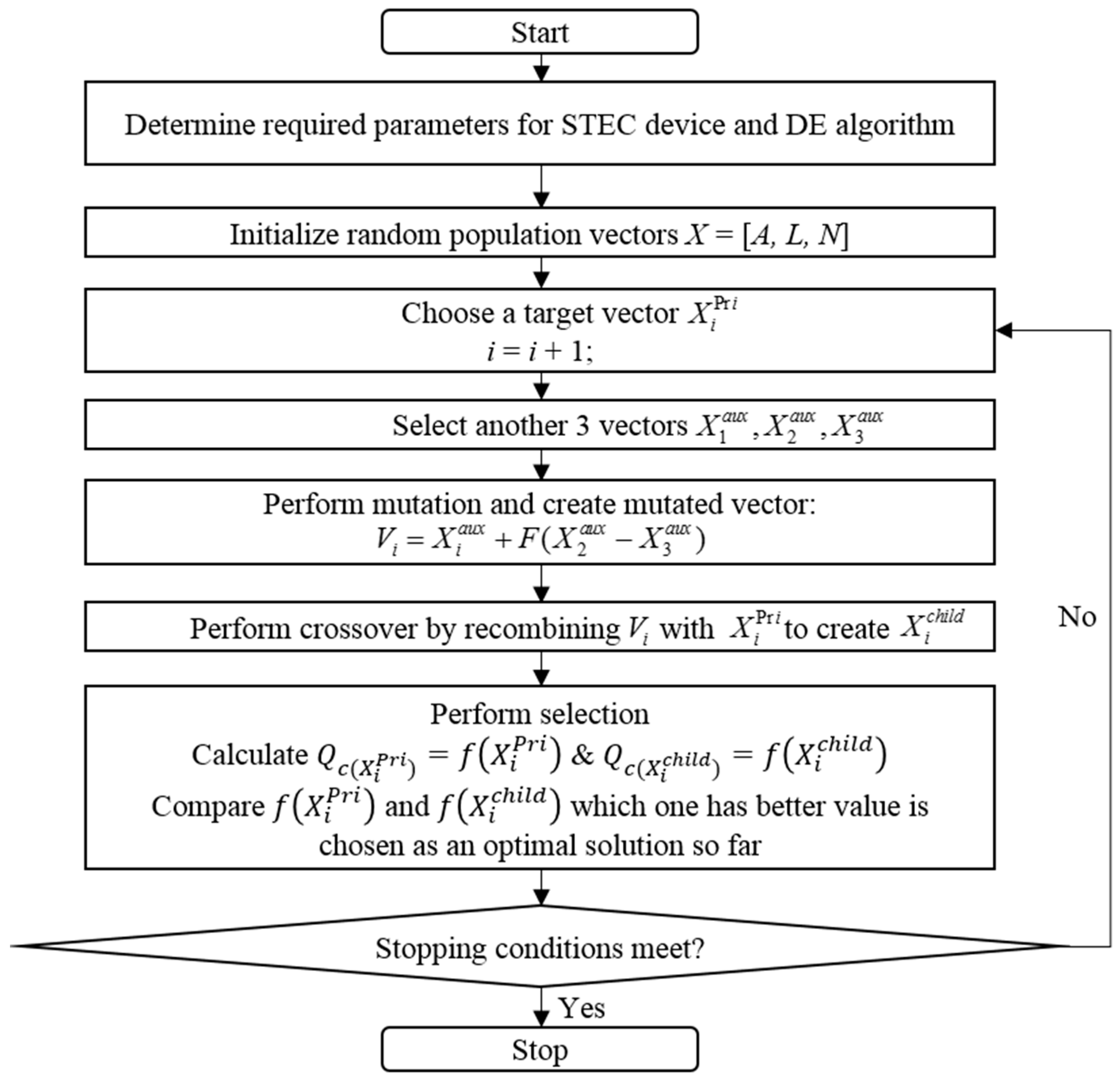
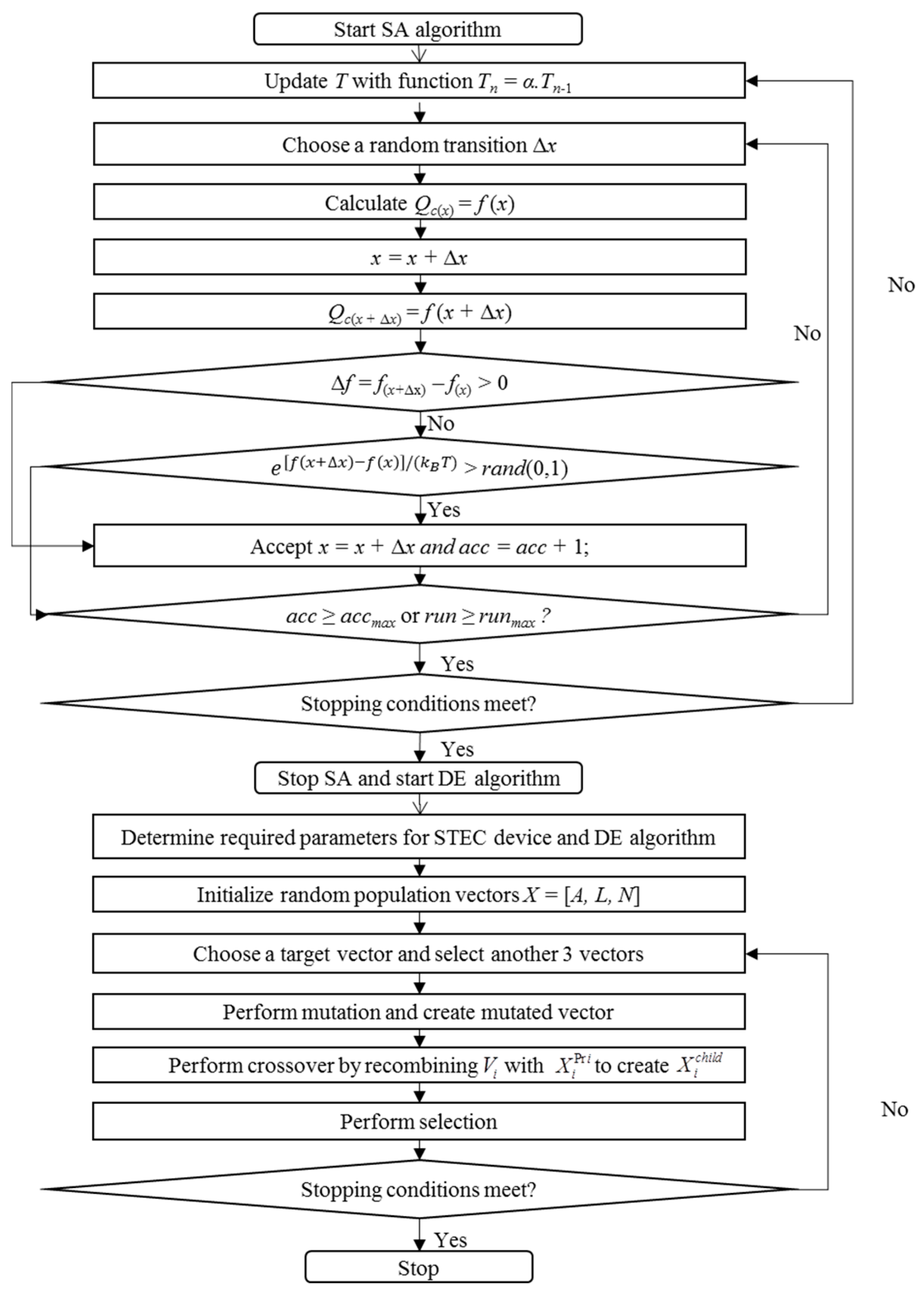
3.4.3. Differential Evolution Algorithm

As introduced by Price and Storn, DE is one of the popular evolutionary metaheuristic algorithms like GA and PSO. DE was divided in ten different strategies, a strategy that works out to be the best for a given problem may not work well when applied for a different problem [48]. DE has been widely employed for solving problems with the features of having many local minima or constraints, being multi-dimensional, nonlinear, flat, non-differentiable and non-continuous. The optimization search of DE proceeds over three operators, which are selection, crossover, and mutation [50]. At the first stage, a population of candidate solutions for the optimization task to be solved is randomly initialized [20]. One target vector $X_i^{\mathrm{Pr}i}$ is randomly selected in the population. For every generation of the evolution process, new individuals are produced by applying reproduction operators: crossover, and mutation. In mutation process, the mutant vector V_i is generated by combining three randomly selected vectors $X_1^{aux},X_x^{aux},X_3^{aux}$ from the population vector excluding target vector $X_i^{\mathrm{Pr}i}$ as in Equation (38):

$$V_i=X_1^{aux}+F(X_2^{aux}-X_3^{aux})$$

(38)

F is the mutation amplification factor, which is a positive real number controlling the rate at which the population evolves. In a crossover process, DE performs uniform crossovers between target vector $X_i^{\mathrm{Pr}i}$ and mutant vector V_i to create trial vector $X_i^{child}$, as in Equation (39). The crossover probability, CR which is used for controlling the fraction parameter values that was copied from the mutant vector must be specified within the range of [0, 1]. For determining which source contributes a given vector, uniform crossover compares CR to the output of rand (0, 1): a uniform random number generator. If the random number generated is equal to or less than CR, the trial vector is inherited from the mutant vector. In other cases, the vector is copied from the target vector:

$$X_i^{child}=\{\begin{array}{l}{V}_i\mathrm{if}\left(\mathrm{rand}\right(0,1)\le CR)\\ X_i^{\mathrm{Pr}i}\mathrm{if}\left(\mathrm{rand}\right(0,1)>CR)\end{array}$$

(39)

Finally, the fitness of the resulting solutions is evaluated in the selection process and the target vector of the population competes against a trial vector to determine which one will be retained in the next generation, as shown in Equation (40). The operation procedure of DE is similar to that of GA but has a small difference with GA in the mutation period.

$$X_{i+1}^{\mathrm{Pr}i}=\{\begin{array}{c}{X}_i^{child}\mathrm{if}f(X_i^{child})<f(X_i^{\mathrm{Pr}i})\\ X_i^{\mathrm{Pr}i}\mathrm{otherwise}\end{array}$$

(40)

The flowchart of the DE algorithm is represented in Figure 8:

Parameter selection of DE is shown in

Table 2. Parameter settings of the DE algorithm.

No.	Parameter	Specified Value
1	Number of population member	P = 30
2	Scaling factor	F = 0.85
3	Crossover probability constant	CR = 1
4	Variable number	D = 3
4	Maximum iteration	imax = 300

, using deterministic rules.

DE selection strategy—DE/rand/1/bin. Scaling factor F is based on the experience of Price and Storn, DE is sensitive to the choice of scaling factor F. The bigger value of F the higher exploration the capability of DE is [51]. A good initial guess is to choose F within the range of [0.5, 1], for example F = 0.85 can be an effective initial choice [12]. It is expressed that the value of F greater than 1 or smaller than 0.4 is occasionally effective. Crossover probability CR, a bigger CR can improve the convergence speed of the algorithm but a smaller CR can make the exploitation capability becomes higher [51]. CR value is chosen from the range of [0, 1] to help maintain the diversity of the population but should be close to 1 for most as [0.9, 1] [12]. When CR = 1, the number of trial solution will be reduced and may lead to stagnation. Only separable problems do better with CR values close to 0 like [0, 0.2] [50]. Number of population P—is also not very critical. An initial guess (10 × D) is a good choice to obtain global optimum [51]. D stands for number of variables. According to the difficulty of the objective problem, the number of population P can be lower than (10 × D) or higher than it to achieve convergence such as 5 × D to 10 × D, 3 × D to 8 × D or 2 × D to 40 × D [12] be consistent with symbols. In the stopping case, the algorithm will stop if total number of function evaluations is above its maximum value i_max = 300.

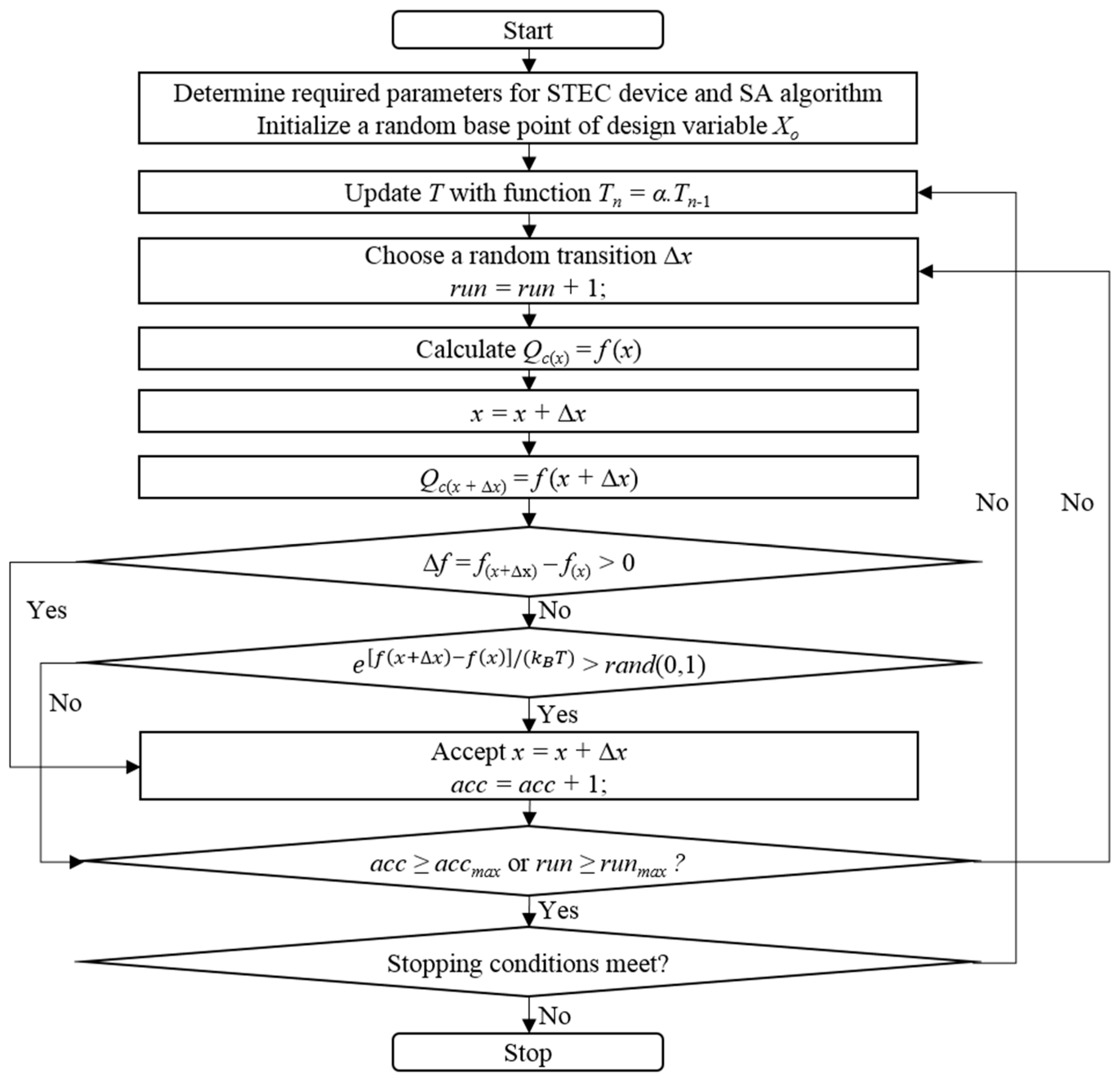
3.4.4. Simulated Annealing Optimization Algorithm

Simulated Annealing (SA) is an algorithm (technique) that can be used for bound-constrained and unconstrained optimization problems [52]. SA is inspired by the physical process of heating a material and then slowly lowering the temperature to decrease defects, by minimizing the system energy in this way [52]. At this point, considered objective function of the problem similar to the energy of a material is then minimized, by introducing a fictitious temperature, as a parameter of the SA [52].

In each iteration of the SA, a new point of x^k+1 is generated randomly within the boundary constraint based on the current point x^k. Distance between the new point and the current point (or the extent of the search) is associated with a probability distribution over a scale, which is proportional to the temperature. Here, SA accepts all new points lowering the objective based on Equation (41), but also, with a certain probability, points that raise the objective, based on Metropolis calculation as in Equation (42), where T_n is the current annealing temperature and k_B is Boltzmann annealing. SA avoids being trapped in local minima by accepting points that raise the objective, and in this way, it can also explore globally for more possible solutions. An annealing schedule is selected for decreasing the temperature systematically during the execution of SA steps. SA reduces the extent of its search to converge to a minimum while the temperature is decreasing.

$$f(x^{k+1})\le f(x^k)$$

(41)

$$\exp \left(-\frac{f\left(x^{k+1}-x^k\right)}{k_B{T}_n}\right)>\mathrm{rand}\left(0,1\right)$$

(42)

The flow-chart of SA algorithm is represented in Figure 9.

Table 3. SA algorithm parameter settings.

No.	Parameter	Specific Values
1	Initial temperature	To = 100
2	Maximum number of runs	runmax = 250
3	Maximum number of acceptance	accmax = 125
4	Maximum number of rejection	rejmax = 125
5	Temperature reduction value	α = 0.95
6	Boltzmann annealing	kB = 1
7	Stopping criteria	Tfinal = 10−10

presents the parameter selection of SA algorithm briefly.

In this study, SA was employed by adjusting its parameters in order to find the optimal design of a TEC. It is widely known that setting good values for the algorithm parameters is extremely important because the whole optimization process depends on that. In this context, the SA parameter settings of are provided in Table 3. The probability of accepting a worse solution of at least 80% of the initial temperature T_o = 100, should be high enough in the first iteration of the algorithm. The temperature is the control parameter in SA as it is decreased gradually while the algorithm steps proceed [53]. Temperature reduction value α = 0.95, temperature decrease function is T_n = αT_n−1, experimentation was realized with different α value: 0.70, 0.75, 0.85, 0.90 and 0.95 [54]. Boltzmann annealing k_B = 1, k_B will be employed in the Metropolis algorithm for calculating the acceptance probability of the points [55]. Maximum number of runs run_max = 250 determine the length of each temperature level T. acc_max = 125 determines maximum number of acceptance a new solution pount and rej_max = 125 determines maximum number of rejection a new solution point (run_max = acc_max + rej_max) [54]. Stopping criteria determines when the algorithm has reached to the objective energy level. The desired or final stopping temperature is T_final = 10⁻¹⁰.

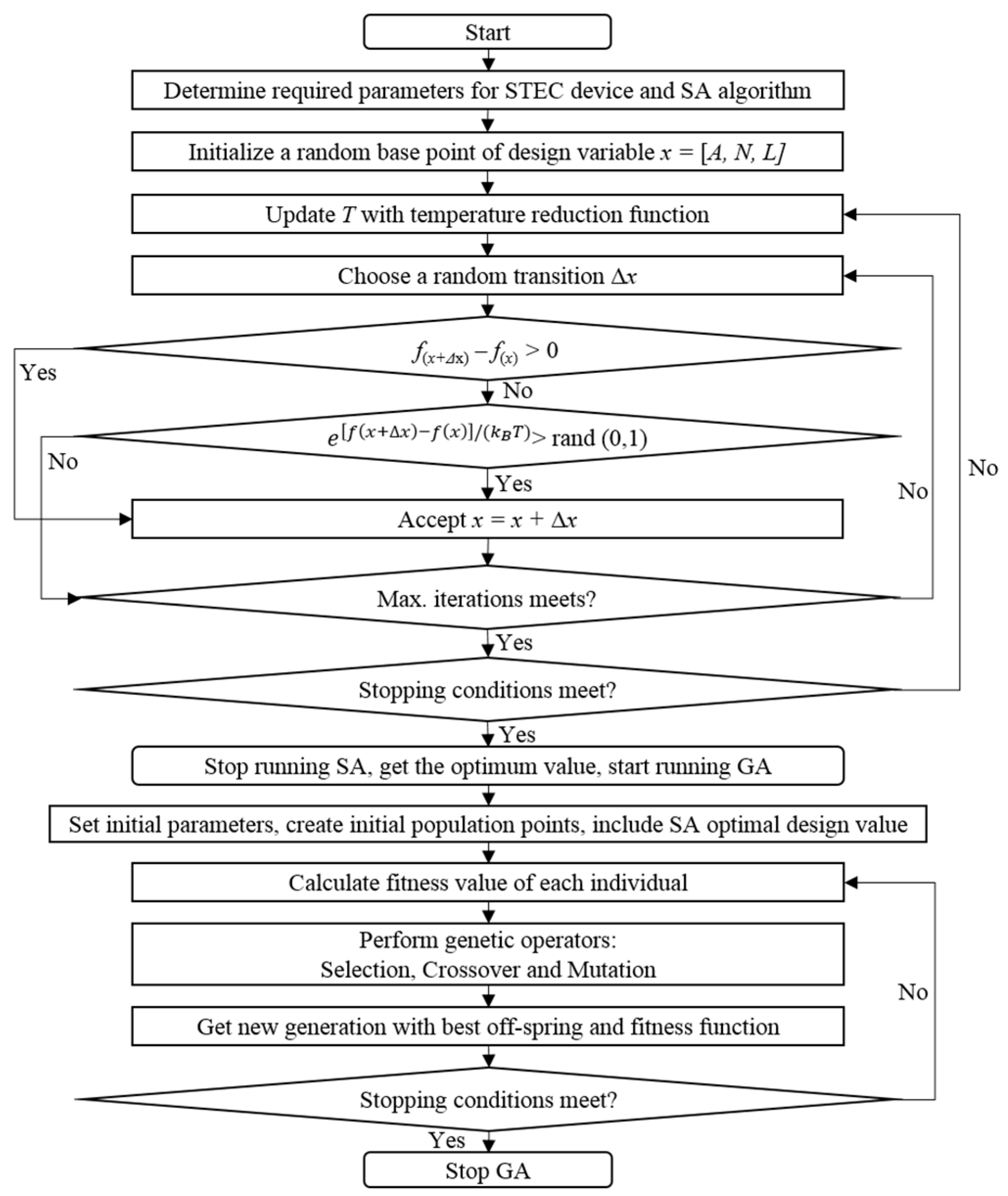
3.4.5. Hybrid Techniques Such as HSAGA and HSADE

Hybrid techniques involve the integration of various metaheuristic algorithms to take their advantages and eliminate their weaknesses to be efficient in finding good solutions [22]. In this study, together with the SA and DE applications, a hybrid technique which is SA combined with GA (HSAGA) is investigated and used to obtain the Pareto optimal point of cooling rate and COP. However, this technique is recommended based on first considering the performance of standalone SA and GA. If they cannot perform well in finding the optimal result of TEC, then a hybrid solution is suggested to be tested and analyzed.

The optimization search of HSAGA consists of two main parts: the first is SA process and the second is a GA process. In MATLAB, the GA algorithm is integrated in an optimization toolbox with fully added parameter settings. Therefore, HSAGA is developed by programming SA and combined with the GA toolbox which is more convenient and easier to code and use its advantages to achieve the highest performance. Firstly, the SA search process is performed until the optimal solutionis obtained. The optimal solution of the SA algorithm then becomes a member in the initial population of GA. The GA search starts to perform its process with three operators: selection, crossover, and mutation. The selection process determines how the individuals are selected for mating, according to their fitness score. The crossover process specifies how the GA combines two individuals to produce a child from crossover, for the next generation. The mutation process specifies how the GA achieves random changes in the individuals within the population for producing mutated children.

HSADE is the combination between SA and DE. SA is implemented first, then the obtained findings from SA is taken into the initial population of DE for selection of the best fitness.

The flow-chart of HSAGA, and HSAGE algorithms—techniques are represented in Figure 10 and Figure 11, respectively.

HSAGA and HSADE are the combination between stand-alone techniques. Therefore, their parameters are the same. Parameter setting of SA and DE are referred in Table 2 and Table 3. In addition, parameter setting for GA is listed in

Table 4. Parameter setting of GA.

No.	Parameters	Specific Values
1	Population size	100
2	Function for fitness scaling	Fitness scaling ranking
3	Function for selection	Selection tournament-4
4	Function for crossover	Arithmetic crossover
5	Crossover fraction	0.6
6	Function for mutation	Mutation Adaptive Feasible
7	Stopping criteria of GA	Maximum number of generations 300

.

From Table 4, it can be understood that the population size, and also maximum number of generations should be set. Here, the generation affects the maximum number of iterations that will be completed by the GA. On the other hand, the population is for determining how many individuals will take place in each generation. It is possible to express that an increase in the population size will increase also accuracy of GA [53] (for finding the global optimum) but it will also cause it to run slowly. At this point, a population size of 100 for 10,000 generations is used generally. Also, selection, crossover, and the mutation operators are used over probabilities in order to get a new set of solutions randomly. For the selection process, there are several options like stochastic uniform, uniform or roulette, tournament, to run for selection. The tournament selection used here chooses each parent by employing four players randomly and then choosing the best individual among them as a parent. The crossover process is done with the arithmetic crossover with fraction 0.6, for producing children, who are weight arithmetic mean of two parents [56] so that the produced children are feasible always with respect linear constraints and bounds. Mutation adaptive feasible is used for the mutation process as satisfying the constraints. At the end, the stopping criteria is set as 300, which is the maximum number of iterations.

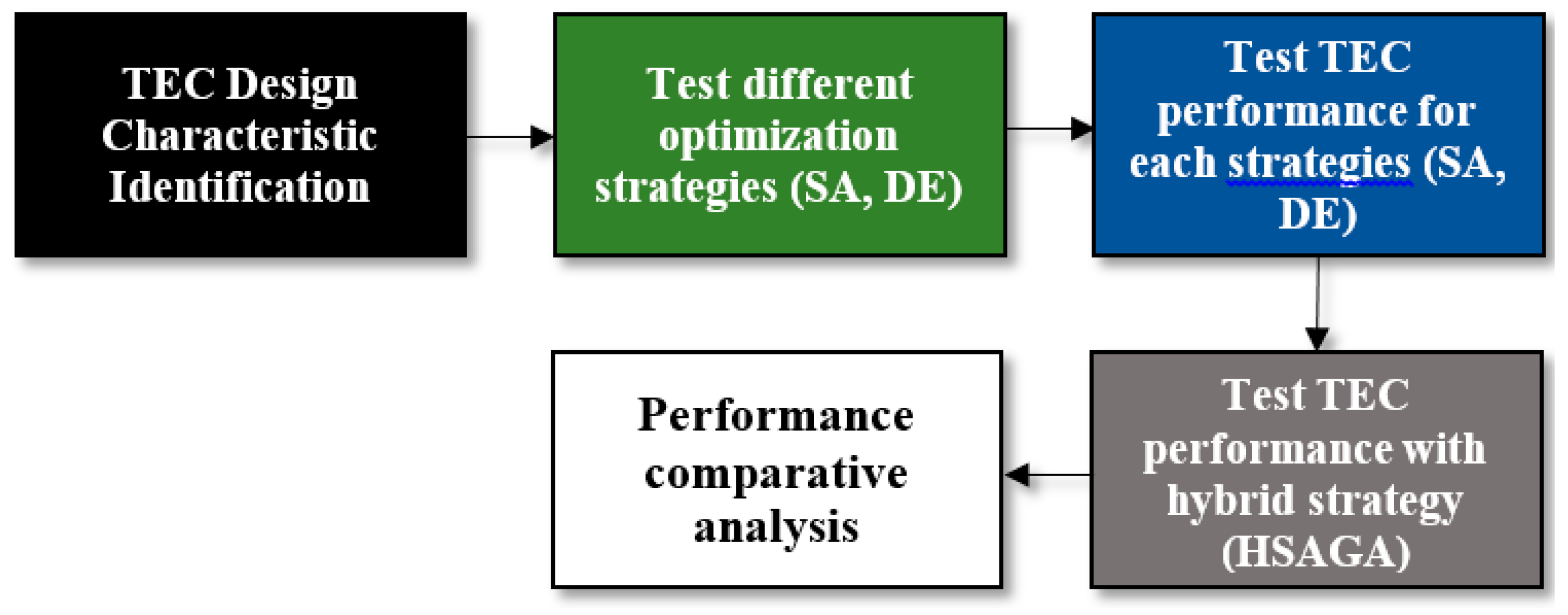
3.4.6. Tests for Evaluating the Algorithms

When a new optimization technique is presented to apply in a specific problem to get the results, at the first its performance should be evaluated and be reported scientifically to see the effectiveness.

Table 5. Test types for evaluating the algorithms.

No.	Test Type	Purpose of the Test
1	Convergence speed test	Measure how fast the algorithm converge by counting the number of iterations
2	Computational effort	Measure time consuming of every running time of optimization technique
3	Stability test	Measure how stable & accurate the algorithm obtain after a number of trial runs
4	Robustness test	Measure ability to realize well many test problems & parameters

lists the test types with respect to its objective to evaluate the performance of SA, DE and hybrid technique.

The testing experiment needs to be implemented by following the pioneers who provided high quality reports regarding computational experiments realized via mathematical programming software. Based on Richard and also some other recent works, some criteria were recommended [51,57,58,59,60,61] to evaluate the effectiveness of optimization techniques as follows:

▪

Fast—the optimization technique has the capability to produce high-quality solutions quicker than other optimization approaches.

▪

Simple—the algorithm code is easy to implement with less parameter setting than other optimization approaches.

▪

Accurate—the optimization technique is able to identify higher quality solutions than other optimization approaches.

▪

High impact—the optimization technique can solve a new or important—remarkable problem more accurately and faster than other approaches.

▪

Robustness—the optimization technique is less sensitive to differences taking place in the problem features, tuning parameters, and data quality, according to other approaches.

Experiments in a computational manner are usually undertaken with the algorithm for comparing the performance provided by different algorithms against the same problems. Therefore, computational experimentation considering the performance of SA and DE when applying in TEC model is necessary to demonstrate that they can provide a good performance, GA which was used to apply in TEC model is used in this research to make the comparison.

3.4.7. Parameter Selection of TEC

For the parameters of a Single-stage Thermo-electric cooler (STEC) we refer to Cheng’s work [29]. In this context,

Table 6. Parameter setting of the STEC model.

No.	Parameters	Description
1	Objective function	Single-objective optimization—Maximize Qc
2	Variables	L—Height of semiconductor element (mm)
		A—Area of semiconductor element (mm2)
		N—Total number of semiconductor elements (unit)
3	Fixed parameter	Th = Tc = 323 °K→Tave = 323 °K
		I = 1 (A)
		rc = 10−8 (Ωm2)
4	Constraints	1. Boundary constraint: - 0.03 mm ≤ L ≤ 1 mm  - 0.09 mm2 ≤ A ≤ 100 mm2  - 1 unit ≤ N ≤ 1111 unit
		2. Inequality constraint:   - Limited total surface area S = 100 mm2   - Production cost of material $385
		3. Equality constraint:  - Minimum requirement COP = 1

lists the parameters of the STEC.

Single objective optimization which considers Q_c as an objective function in this test. T_h and T_c were both set as 323 °K, hence the temperature difference between the hot and cold side of the STEC is 0 °K. ΔT = 0 °K is not practical for our refrigeration aim but it can get the maximum Q_c for cooling aim for the same applied current and TEC geometry [31]. Based on that, the average temperature between hot stage and code stage T_ave is 323 °K, and the material features of the STEC are then calculated via Equations (18)–(20). STEC is located in a confined volume over a total area of S = 100 mm² and a height of H = 1 mm. The maximum cost of the material is $385. COP requirement can be ignored to be able to determine the global maximum Q_c or can be consider as a satisfied condition in practical design [31]. Design variables are x = (L, A, N) and are put in a boundary constraint (L_min–L_max, A_min–A_max, N_min–N_max). L_min is based on the technological limitations in manufacturing TEC semiconductor elements which is 0.3 mm, L_max= H = 1 mm. A_min is also constrained because of the technological limitation of semiconductor elements, which is $L_{\min }^2$ = 0.09 mm², and A_max = S = 100 mm². N depends on the area of a single semiconductor element, hence, with a defined total area of STEC S = 100 mm², N_min = 1 and N_max = S/A_min = 1111 (unit). The effect of resistance (electrical) on junctions r_c is taken into account with the value of 10⁻⁸ Ωm².

On the other hand, the parameter settings of the Two-stage Thermo-Electric Cooler (TTEC) are taken from Cheng’s work [30].

Table 7. Parameter setting of the TTEC model.

No.	Parameters	Description
1	Objective function	Single-objective optimization—Maximize Qc,c or maximize COP
2	Variables	Ic—Input current to the cold stage (A)
		Ih—Input current to the hot stage (A)
		r—ratio number for semiconductor elements between the hot stage and the cold stage
3	Fixed variable	Nt = 100 (unit)
		G = 0.0018 m
		Th,h = 300 °K
		Tc,c = 240 °K
4	Boundary constraint	4 A ≤ Ih ≤ 11 A
		4 A ≤ Ic ≤ 11 A
		2 ≤ r ≤ 7.33

presents the parameter selection regarding the TTEC.

A first type TTEC with electrically connected in series (I_h = I_c) is used for single objective optimization which consider Q_c,c as an objective function in this test. The TTEC is used to produce a temperature T_c,c = 210 °K when the hot stage is maintained at T_h,h = 300 °K. The design variables are x = (I_c, I_h, r) and are put in a boundary constraint (I_cmin–I_cmax, I_hmin–I_hmax, r_min–r_max). Value settings for this boundary constraint are referred from [33]. The total number of semiconductor elements of TTEC is N_t = 100 units and the ratio for cross sectional area to the length of semiconductor element is G = 0.0018 m.

In this part, five case studies are done to test the performance of SA and DE optimization technique with the test types presented in the Table 4. These test cases are as follows:

▪

Test case-1: The STEC model is optimized under the constraints of total limited area S = 100 mm² and maximum cost of material $385. The parameter setting follows Table 6 but the requirement of COP is ignored.

▪

Test case-2: The STEC model is optimized under the requirement of satisfying the condition that the COP is equal to 1. The purpose is to test the capability of solving non-linear equality constraint problem of both algorithms.

▪

Test case-3: The STEC model is optimized under all the constraints in test cases 1 and 2. The capability of handling both inequality and equality constraints is tested to see which algorithm performs slightly better. The parameter setting follows Table 6.

▪

Test case-4: The TTEC model is optimized with considering Q_c,c as objective function under boundary constraint conditions, not too complicated as compared to the above test cases. The parameter setting follows Table 7.

▪

Test case-5: The TTEC model is optimized with considering COP as objective function. The parameter setting follows Table 7.

4. Applications—Tests

Based on the condition setting for TEC and parameter setting for the algorithm SA, DE and hybridized technique, this section presents the comparison between the algorithms based on the obtained value of the objective function. The best algorithm is evaluated from the analytical result and choose for multi-objective optimization.

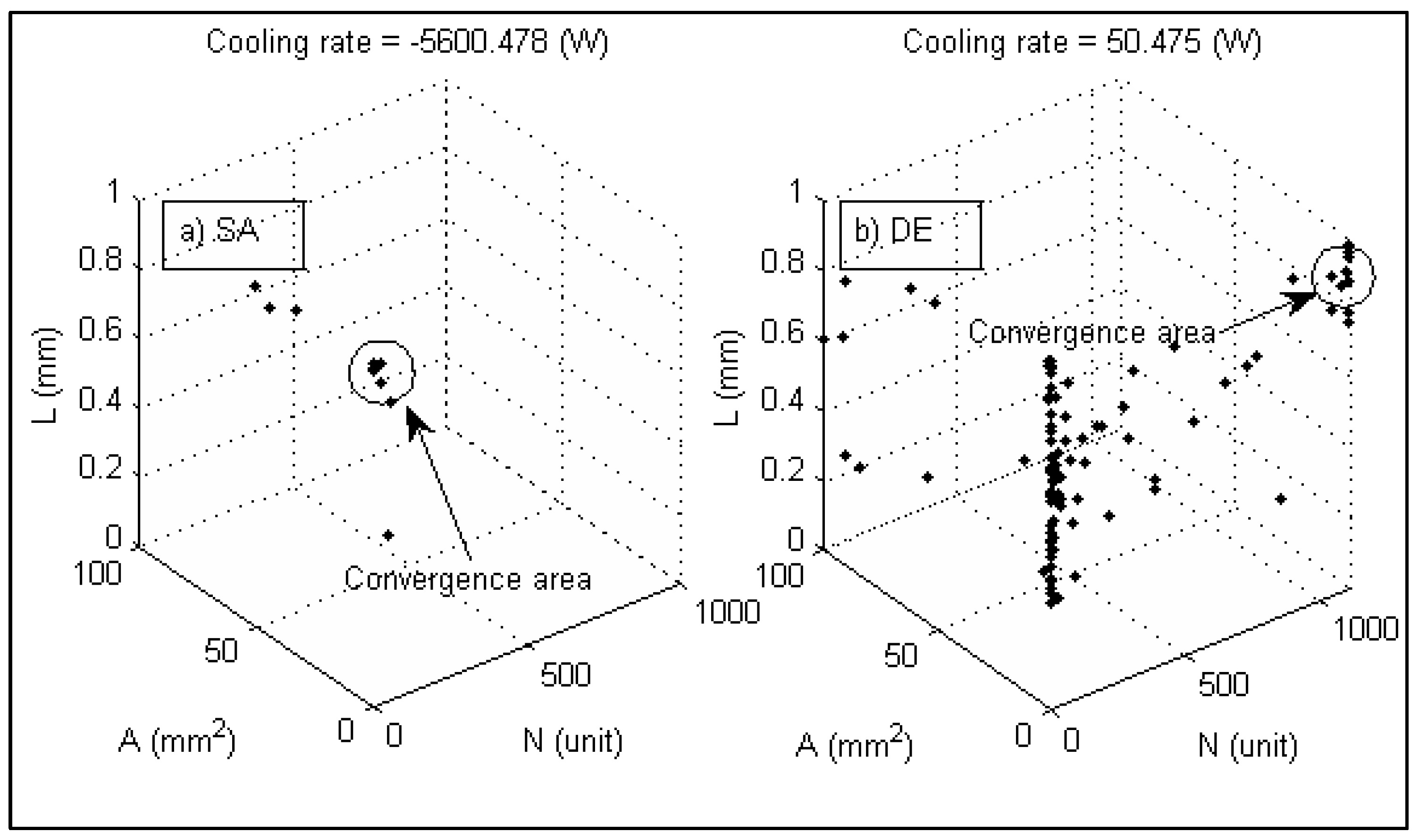
4.1. Convergence Speed Test

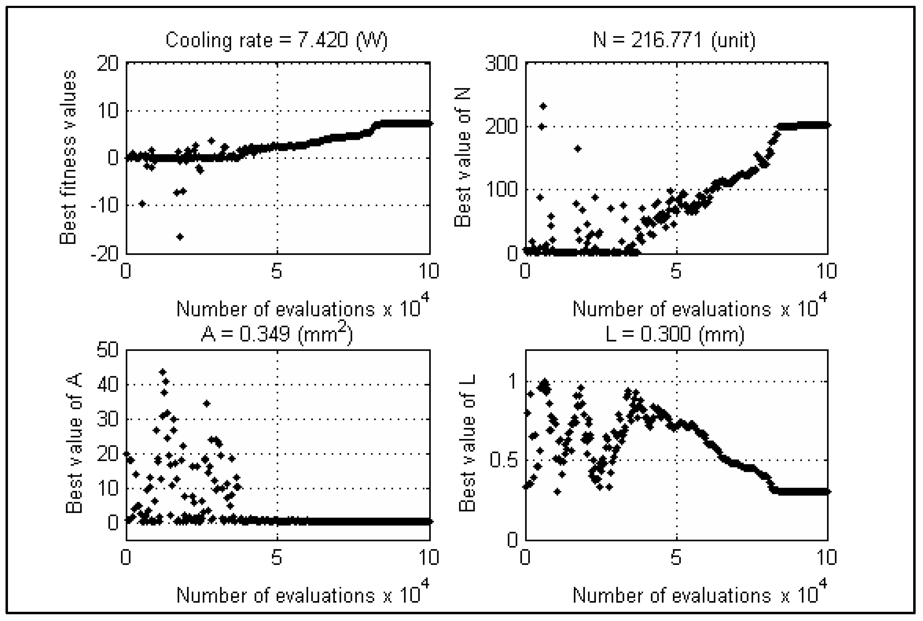
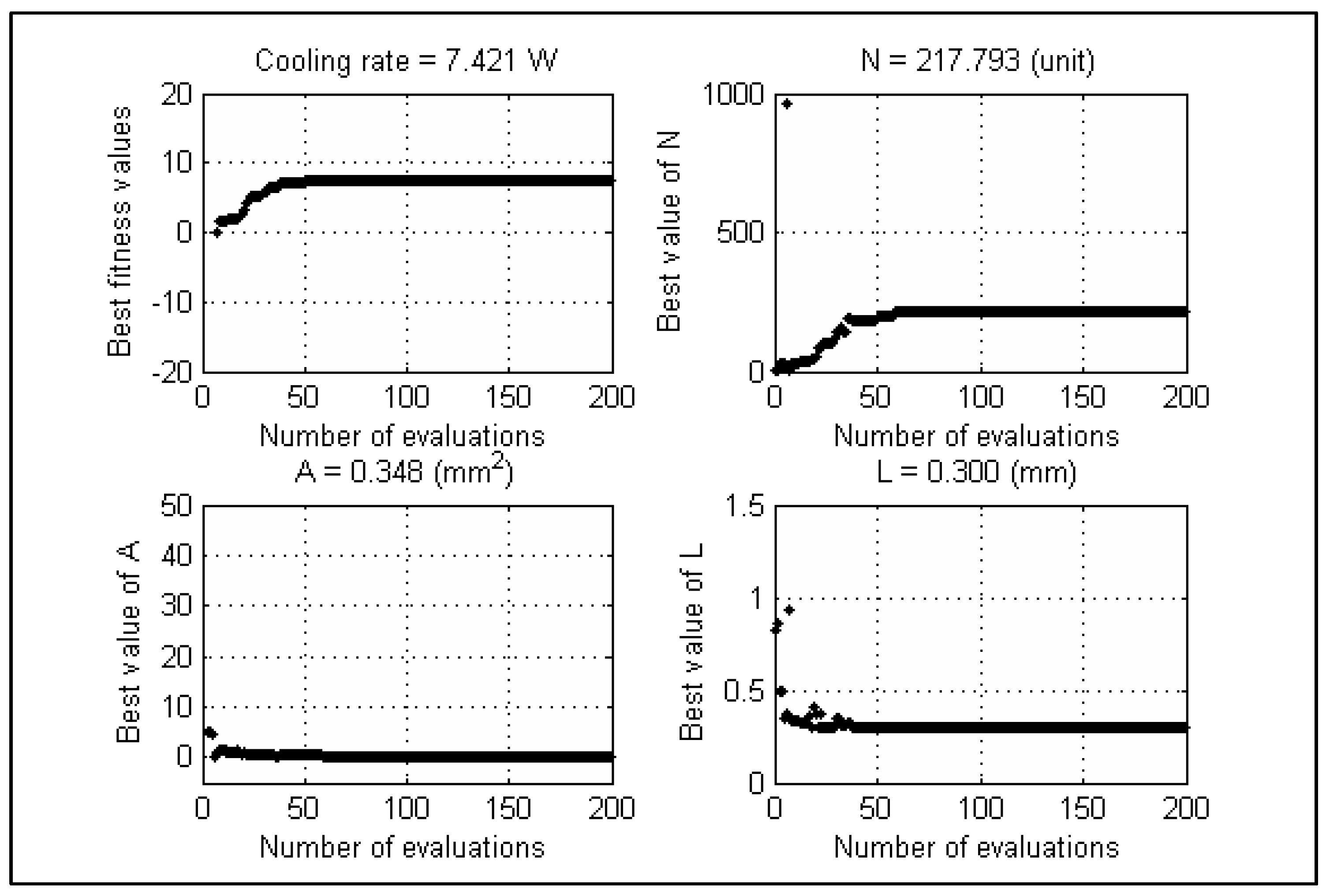
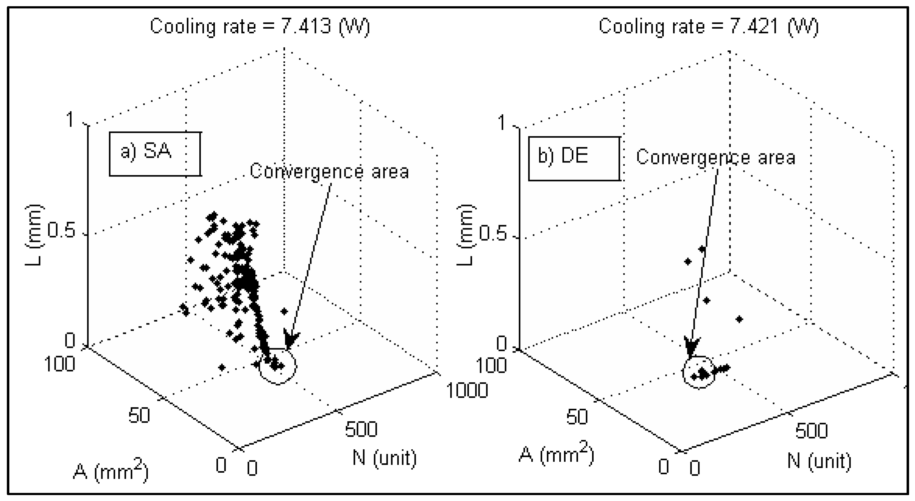
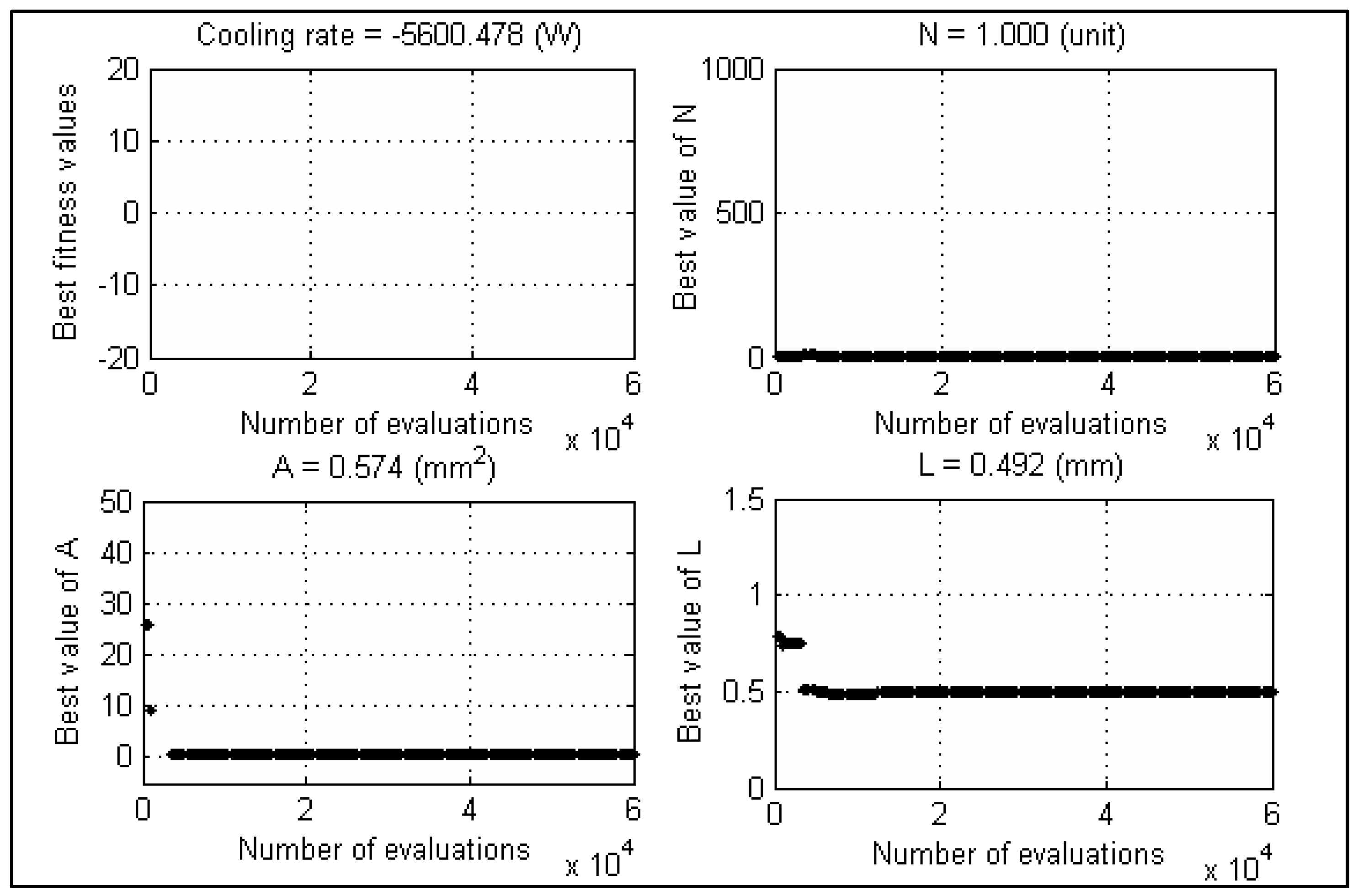
Obtained findings within the convergence speed tests can be expressed briefly as follows by considering also graphical outputs from the related applications—tests.

4.1.1. Test Case-1

Figure 12 represents the convergence curves of the maximum cooling rate, the optimal design parameter (A, L, N) using the SA algorithm. The points with black color are the accepted optimal solutions within the search process. The optimal maximum cooling rate is 7.420 (W). Optimal design parameters (A, L, N)₁ = (0.349 mm², 0.3 mm, 217 units). The obtained result satisfies all constraints (A₁N₁ = 75 mm² < S = 100 mm², cost of material = $381.15 < cost_max = $385). The SA algorithm converged after 80,000 iterations. Computational time of the algorithm until it meets the stopping condition is more than 30 s.

Figure 13 shows the convergence of DE. DE produces the same optimal result as the SA approach. The optimal maximum cooling rate is 7.421 (W). Optimal design parameters (A, L, N)₂ = (0.348 mm², 0.3 mm, 218 units). The obtained result satisfies all constraints (A₂N₂ ~ 76 mm² < S = 100 mm², cost of material ~ cost_max = $385). The DE algorithm converges promptly after 45 iterations. Computational time until it meets the stopping condition is 7.5 s. It can be seen clearly that DE performs faster than SA in the same TEC system setting. From the search processes of both algorithms, the maximum cooling rate increases until it meets optimal value, meanwhile the length of semiconductor element L decreases to the lower bound of the boundary constraint. This phenomenon matches Huang’s research [31]. As it can be seen in Equation (4) provided before that with the same operating condition (I = 1 A, T_h = T_c = 300 °K (ΔT = 0)), a small length of semiconductor element makes the Joule heating weak by leading to a large cooling rate.

Figure 14 shows the 3D search of optimal points of design parameters (A, L, N), the points with black color are the accepted optimal solutions within the search process, and the convergence area of the algorithm is pointed out. As it can be understood that both algorithms produce the same optimal findings, hence, they converge at the same position on the graph. The search area of SA which is inside the boundary is fairly wide and the search area of DE is narrower than the SA’s one. An explanation for that result is as follows: in first stages, the annealing temperature T is still high which leads to a high probability of accepting the neighbor points that have worse fitness values. Many new points are created with better or even worse fitness value. For DE, only individuals with better fitness values can be selected as the optimal values.

4.1.2. Test Case-2

This test doesn’t consider the limitation of the total area and cost of material, just the boundary constraint. Therefore, it’s useful to check how big the cooling rate that can be achieved with a required COP in a defined system condition. SA get trapped in a local optimum when trying to find an optimal value of the maximum cooling rate which satisfies the condition of COP = 1. As it can be seen in Figure 15, the optimal maximum cooling rate obtained at negative value. Obtained optimal design parameters (A, L, N) of STEC is not valid. There are a few points of the search area of the design parameters, they reflect the weak escape capability from local optima of SA.

DE can perform well and find the optimal result under the equality constraint condition. As shown by Figure 16, the optimal maximum cooling rate is 50.475 (W). Optimal design parameters (A, L, N)₃ = (0.553 mm², 0.417 mm, 1111 units). The obtained result satisfies the constraints (within the boundary constraint, calculated COP ~ 1). STEC can produce a significant high cooling rate with respect to a required COP but not practical. To produce this STEC module, the minimum required area of STEC should get S_min = A₃N₃ = 614.383 mm²and the minimum cost of material should get cost_min = $4340 which is very costly. The algorithm converges after 175 numbers of evaluation. Computational time until it meets the stopping condition is around 7.5 s.

Figure 17 shows the 3D search of optimal points of design parameters (A, L, N), the points with black color are the accepted optimal solutions, and the convergence area of the algorithm is pointed out. Because it takes more iterations to converge to the optimal solution, more points are reflected in the figure as compared to its performance in Test case-1.

4.1.3. Test Case-3

This test case is useful for designers to achieve an optimal cooling rate with respect to a required COP. From Figure 18, the optimal maximum cooling rate is 6.587 (W). Optimal design parameters (A, L, N)₄ = (0.522 mm², 0.3 mm, 145 units). The obtained result satisfies all constraints (A₄N₄ = 75.69 mm² < S = 100 mm², cost of material = $384.7 < cost_max = $385). The algorithm converges after 155 numbers of evaluation. Computational time until it meets the stopping condition is 7.55 s. In Cheng’s work [29], by using the same setting of STEC model, the achieve the optimal design (A, L, N)₅ = (0.56 mm², 0.3 mm, 134 units) with the cooling rate is 5.62 (W). These values show the benefit of DE when can find a better set of design parameters which yield larger fitness value. This issue is discussed and analyzed later.

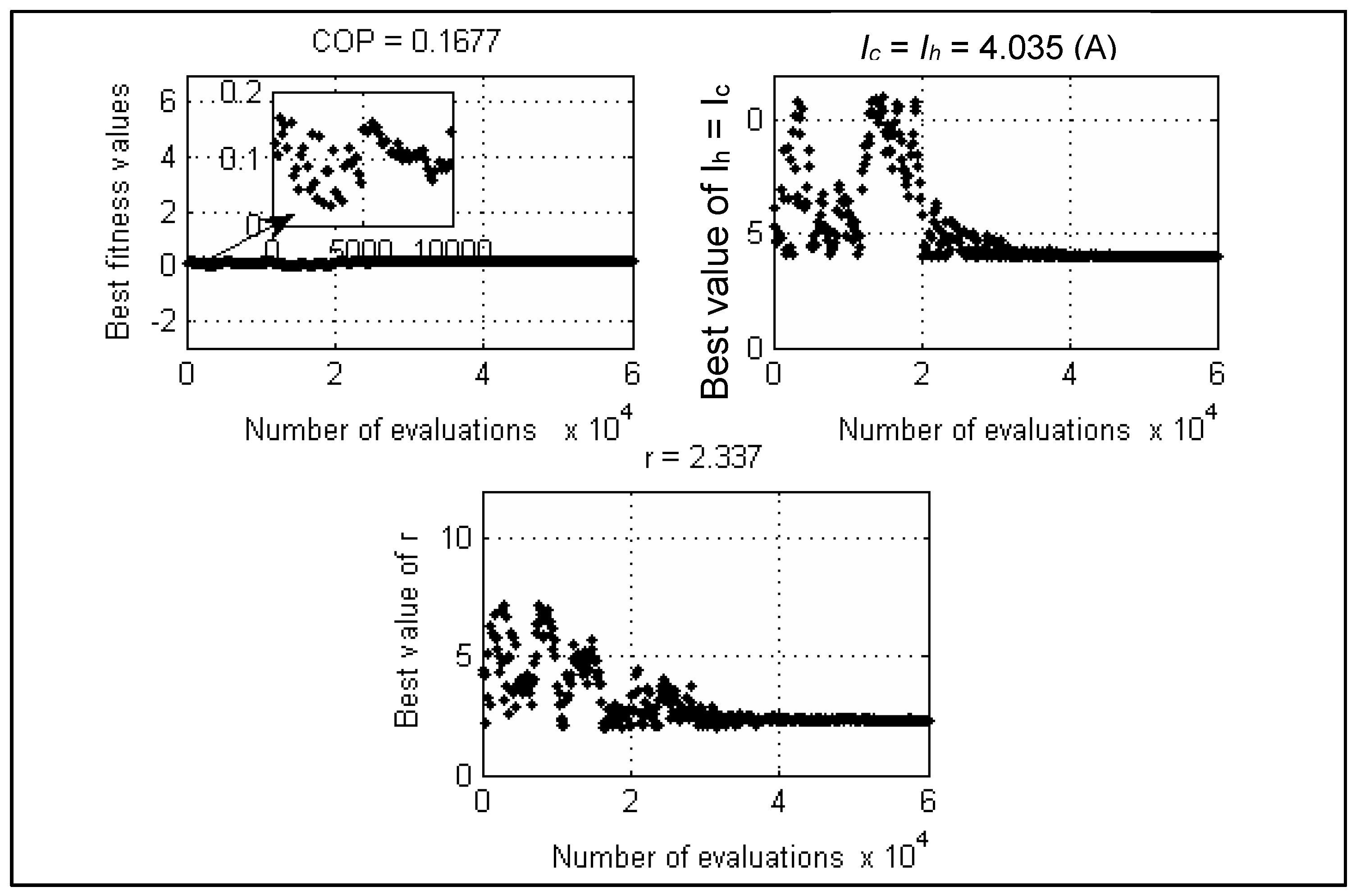
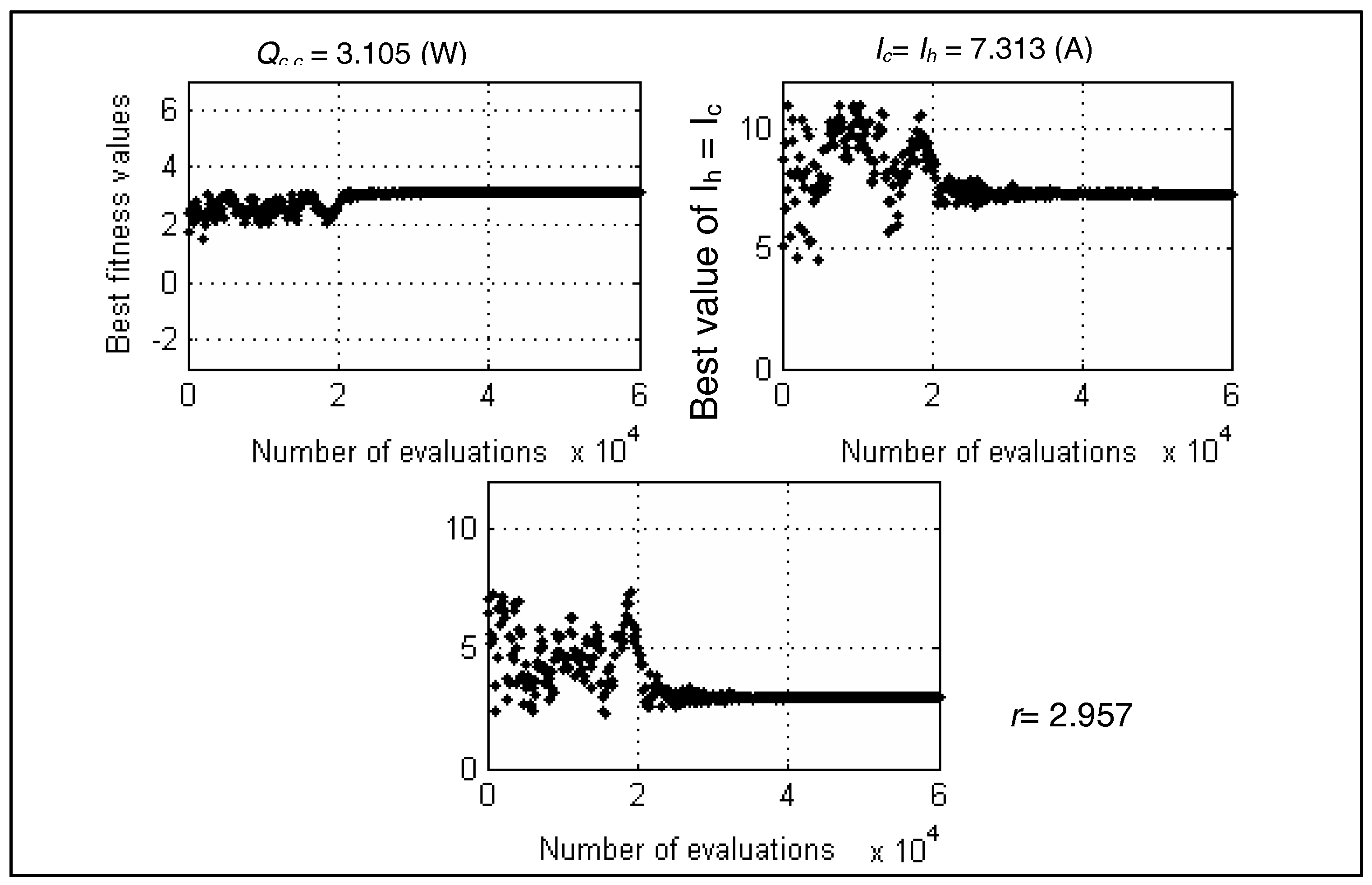
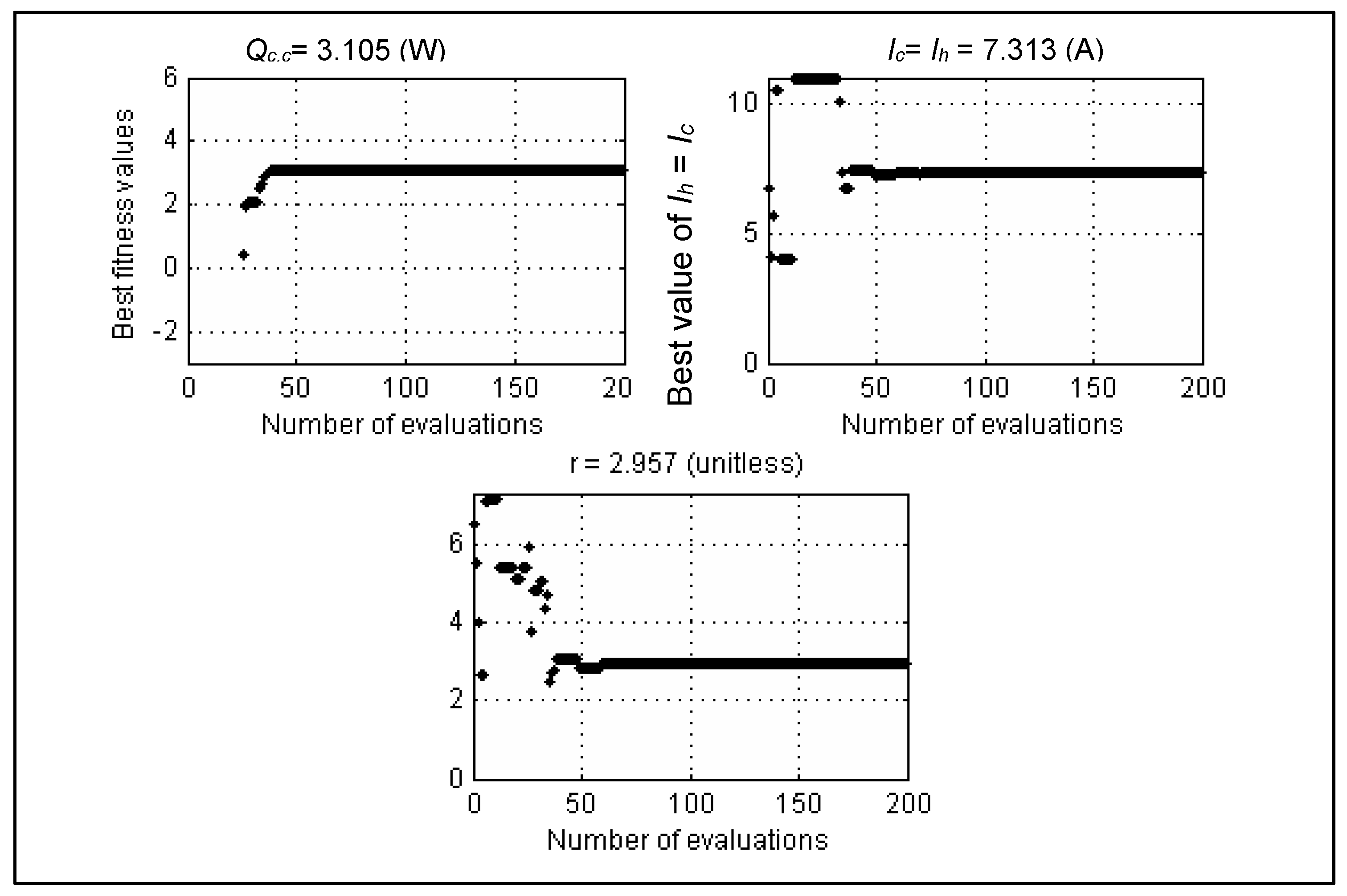
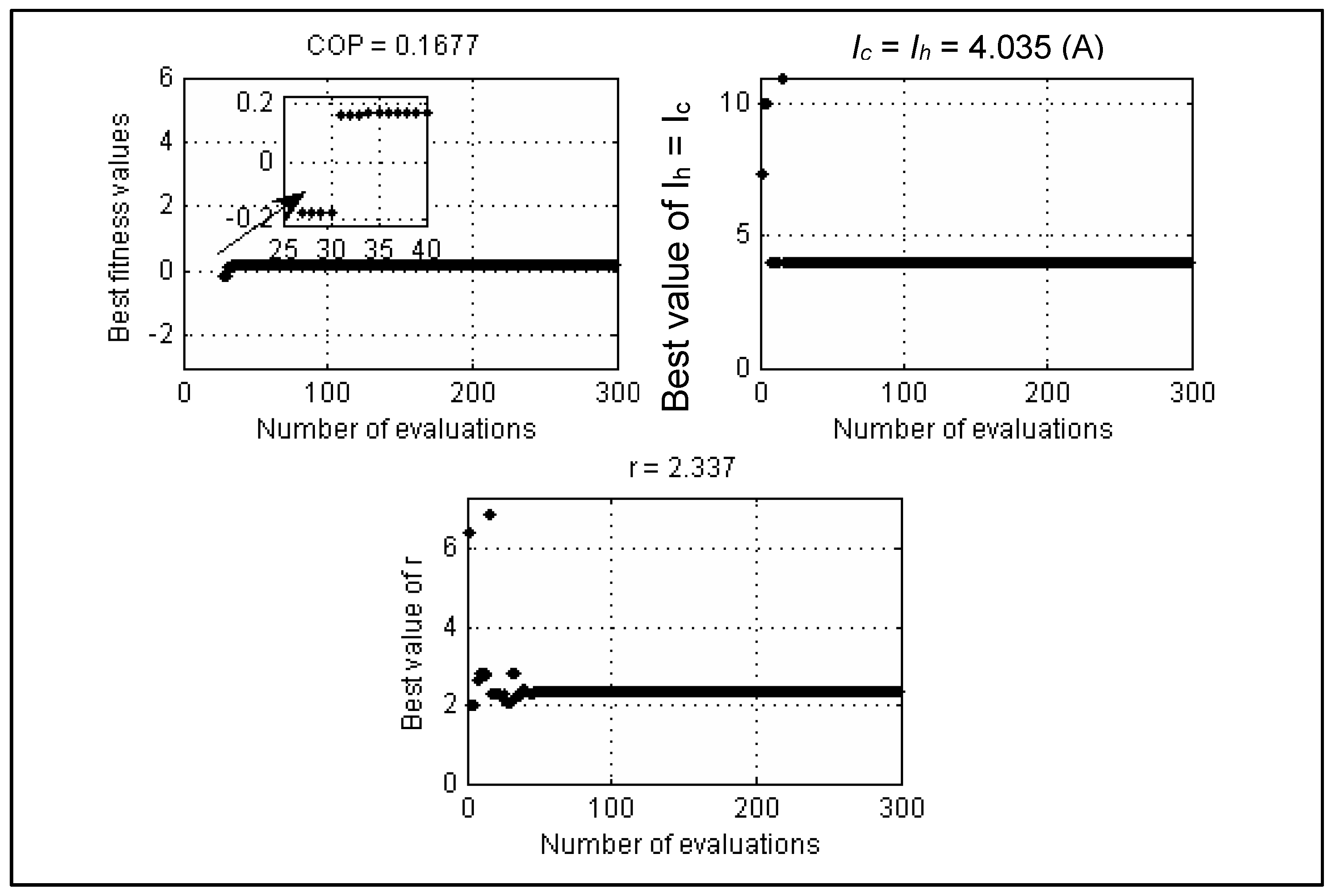
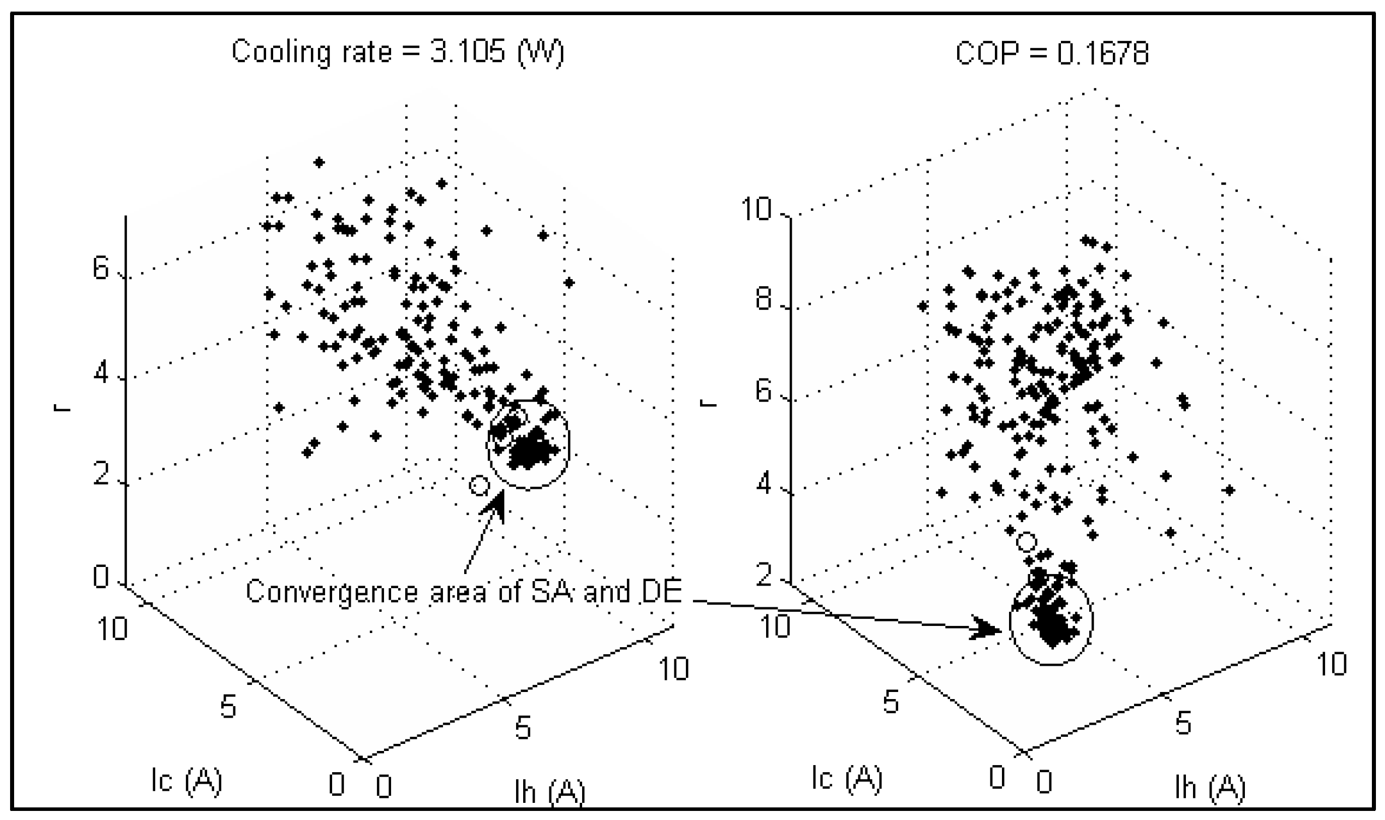
4.1.4. Test Case-4 and Test Case-5

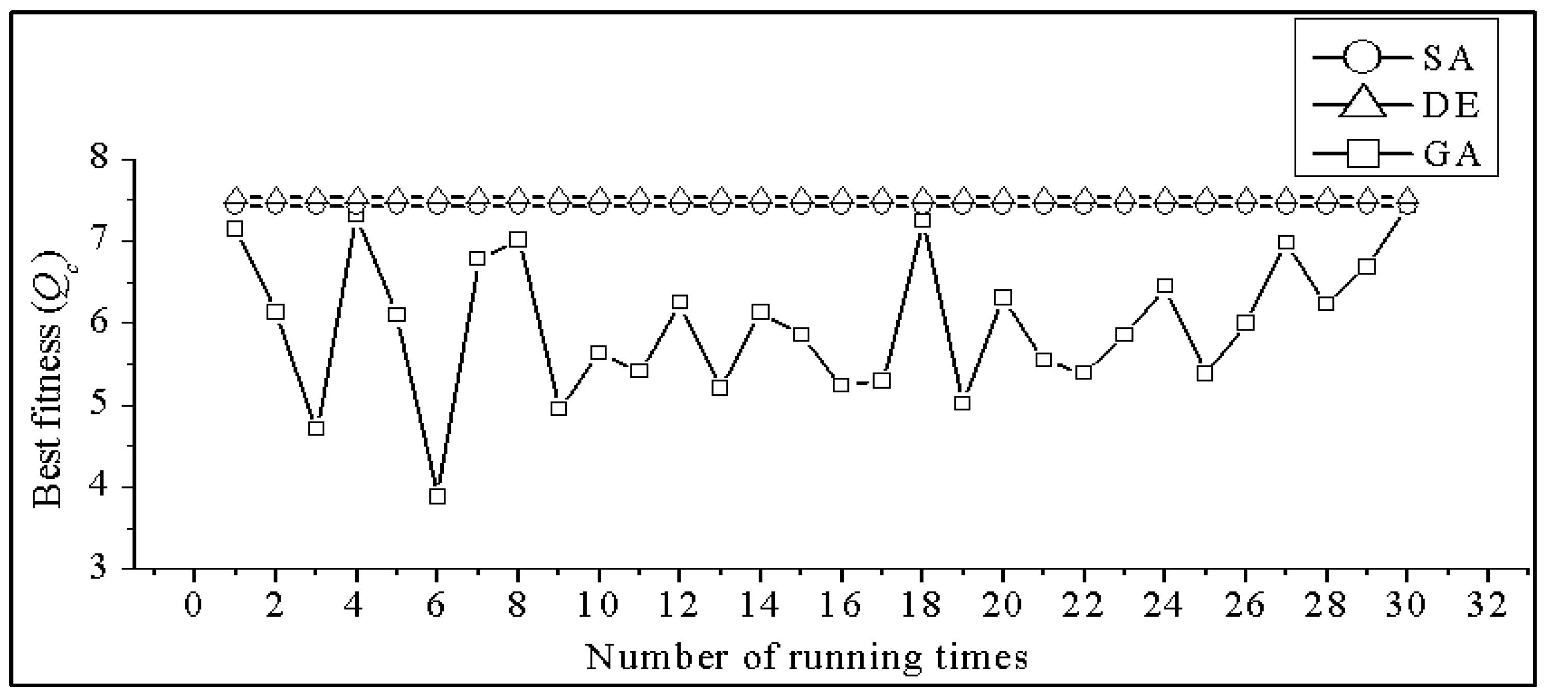
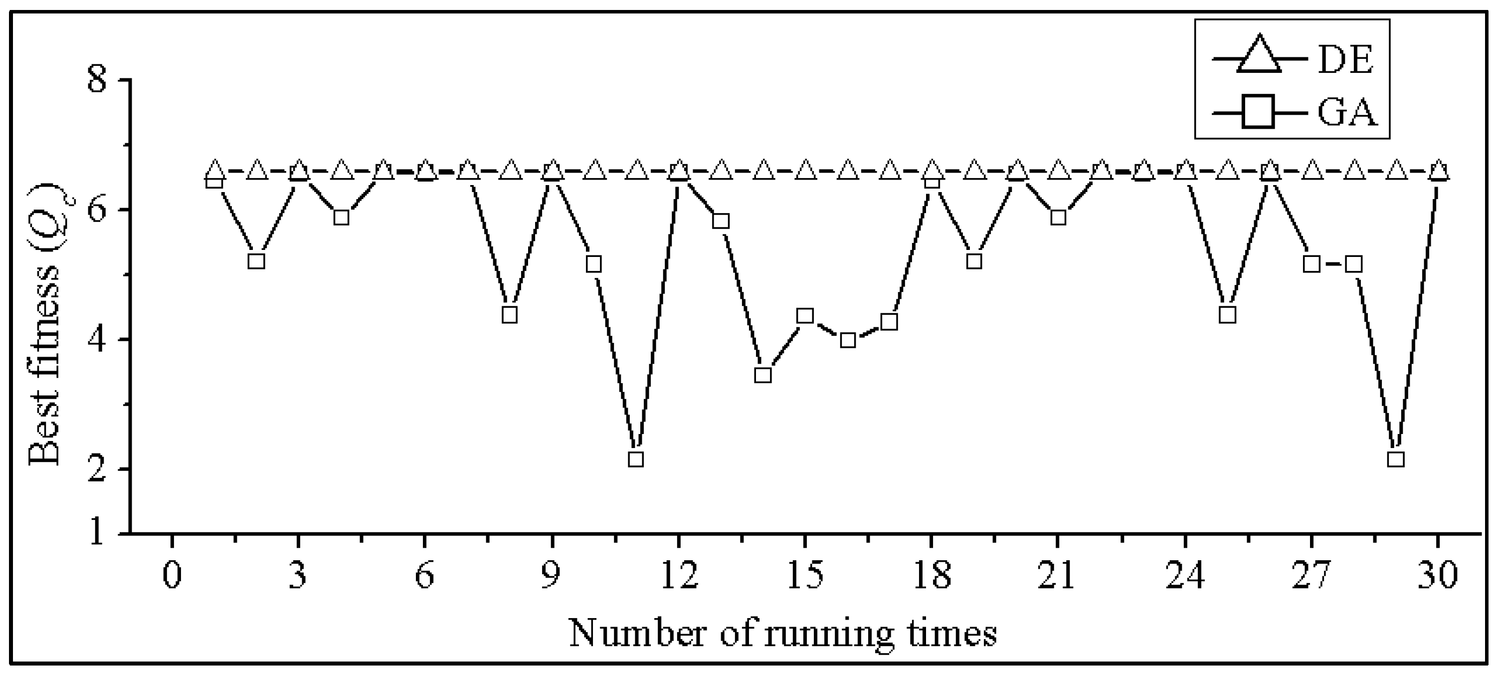
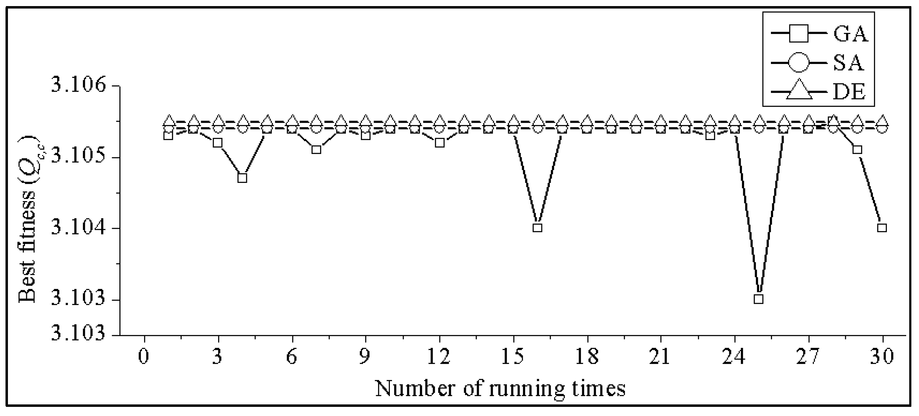
In this test case, SA and DE produce exactly same optimal findings. As shown from Figure 19, Figure 20, Figure 21 and Figure 22, optimal Q_c,c is 3.105 (W) with respect to optimal design parameters (I_h, I_c, r)₁ = (7.313 (A), 7.313 (A), 2.957). Optimal COP is 0.1677 (W) with respect to optimal design parameters (I_h, I_c, r)₂ = (4.035 (A), 4.035 (A), 2.337). Obtained findings of the two test cases satisfies the boundary constraint.

In both test cases, the SA algorithm converges after 42,000 numbers of evaluation over approximate 80,312 total number of evaluations. Computational time until it meets the stopping condition is 66 s. The DE algorithm converges after 100 iterationsof atotal number of 300. Computational time until it meets the stopping condition is 35 s. It’s obvious that the speed of finding the optimal solution using the DE approach is faster than the SA approach.

Figure 23 shows the 3D search of optimal points of design parameters (I_h, I_c, r), the points with “.” symbol re the accepted optimal solutions within the search process of SA, the points with “o” symbols are the accepted optimal solutions within the DE search process. The convergence area of design variables of the two algorithms in the two different test cases is pointed out. As it can be observed that for every test case which is maximizing cooling rate or maximizing COP, both algorithms produce the same optimal findings, hence, they converge at the same position on the 3D-figure. The search area of SA, which is inside the boundary is fairly wide and the search area of DE is narrower than the SA’s one. Compared with Xuan’s work [34] using an analytical method and Cheng’s work [30] using a GA method to find the optimal result of a TTEC, when optimizing the cooling rate, optimal (I_h, I_c, r)₃ = (7.425 (A), 7.425 (A), 2.846) with Q_c,c = 3.08 W. For optimizing COP, optimal (I_h, I_c, r)₄ = (4.054 (A), 4.054 (A), 2.125) with COP = 0.165. DE and SA both produce reliable searches.

4.2. Stability Test

Generally, a metaheuristic algorithm—technique may not converge to an exact solution in every random run performed, hence, it is not possible to accurately evaluate their performances considering only a single run. In contrast, many runs should be realized for every case study of a TEC system setting in order to get an accurate finding—idea regarding the stability of the algorithm. In order to achieve that, SA and DE are coded in theMATLAB 2013a platform and then we run 30 different runs on a computer system (equipped with the Windows 7 OS, an Intel^® Core™ i5-3470 @ 3.2 GHz CPU and 4GB DDR RAM). Case studies are designed for STEC and TTEC to conduct this test following the above test cases. COP is an equality constraint condition which is considered in Test case-3, hence, it is unnecessary to do the Test case-2. Moreover, Test cases 1, 3, 4 and 5 are used for partial results which produce the TEC design based on a literature review.

• Test case-1: Best fitness of STEC after 30 trial runs under two in equality constraints using GA, SA and DE.
• Test case-3: Best fitness of STEC after 30 trial runs under three constraints using GA and DE. SA can’t perform this test under equality constraints.
• Test case-4: Optimal Q_c,c of STEC after 30 trial runs using GA, SA and DE.
• Test case-5: Optimal COP of STEC after 30 trial runs using GA, SA and DE.

In order to evaluate—compare—the performances of SA and DE, GA is run on with the same condition settings in the four test cases. The lowest value, average value, best value, and standard deviation value of the objective function with respect to every technique are provided in

Table 8. Test case-1: Obtained data after 30 trial runs.

Technique Used	GA	SA	DE
Test case 1	Qc (W)	Qc (W)	Qc (W)
Standard deviation of best fitness	0.8616	0.0025	0
Average value of best fitness	5.982	7.417	7.421
Minimum value of best fitness	3.880	7.410	7.421
Maximum value of best fitness	7.417	7.420	7.421

,

Table 9. Test case-3: Obtained data after 30 trial runs.

Technique Used	GA	SA	DE
Test Case-3	Qc(W)	Qc(W)	Qc(W)
Standard deviation of best fitness	1.3251	SA can’t solve this test case	0
Average value of best fitness	5.487		6.596
Minimum value of best fitness	2.154		6.596
Maximum value of best fitness	6.595		6.596

and

Table 10. Obtained data after 30 trial runs.

Technique Used	GA		SA		DE
Test cases 4 and 5	Qc,c (W)	COP	Qc,c (W)	COP	Qc,c (W)	COP
Standard deviation	5.5 × 10−4	8.584 × 10−5	0	0	0	0
Ave. of best fitness	3.1052	0.1677	3.1055	0.1677	3.1055	0.1677
Min. of best fitness	3.1030	0.1673	3.1055	0.1677	3.1055	0.1677
Max. of best fitness	3.1055	0.1677	3.1055	0.1677	3.1055	0.1677
Ave. computational time	18 s	18 s	66 s	66 s	48 s	48 s

. Figure 24, Figure 25, Figure 26, Figure 27 and Figure 28 present the graphs illustrating the best fitness after 30 trials for Test cases 1, 3, 4 and 5.

In test case-1, as shown in Table 8 and Figure 24, the highest achievable best fitness is 7.421 W which is obtained by the DE approach, followed by SA and GA which produce similar values Q_c = 7.420 Wand Q_c = 7.417 W, respectively. The smallest achievable best fitness is Q_c = 5.982 W which is obtained by the GA approach, followed by SA and DE which produce different values 7.417 W and 7.421 W. The average best fitness values obtained by the GA, SA and DE approaches are 3.880 W, 7.410 W and 7.421 W, respectively. As it can be seen in the related figure, in every iteration, DE performs a bit better than SA in this test case after 30 trial runs, and SA and DE both have slightly better performance than GA.

In Test case-3, as seen from Table 9 and Figure 25, SA cannot solve this problem, and the highest achievable best fitness of this test case is Q_c = 6.596 W which is obtained by the DE approach, followed by GA which produces nearly the same value Q_c = 6.595 W. The smallest achievable of best fitness is Q_c = 5.487 W which is obtained by GA’s approach, worse than DE which produces Q_c = 6.596 W. The average value of best fitness obtained by the GA and DE approaches is Q_c = 2.154 W and Q_c = 6.596 W, respectively. DE obviously performs better quality than GA.

Through these test cases, GA seems less effective, producing a lower average cooling rate than the others. To analyze this in more depth, the standard deviation of the best fitness is calculated to measure the dispersion of the data from the mean value. The more spread apart the data, the higher the deviation. As shown in Table 10, in every trial run, for both Test cases 4 and 5, DE produces the same quality of cooling rate, hence, the standard deviation of the best fitness obtained using the DE approach is exactly equal to 0. The obtained findings after 30 trials by using GA’s approach are more oscillation because the achieved best fitness after every running time is quite distinct, with the average value of best fitness is lower than using DE’s approach, but higher standard deviation such as 0.8616 W in Test case-1, 1.3251 W in Test case-3. GA avowedly shows less stable than DE. When using SA, in Test case-1, the findings after 30 trials have a bit oscillate, not perfect as DE but much better than GA with standard deviation is 0.0025 W. In Test cases 4 and 5, SA make a good performance when yield the standard deviation values same with DE which is equal to 0. Using GA is hard to find good optimal findings, using SA can solve a limited issue with higher stability and the ability to find global optimum than GA. DE is an algorithm to find optimal findings of STEC with the highest stability and reliability.

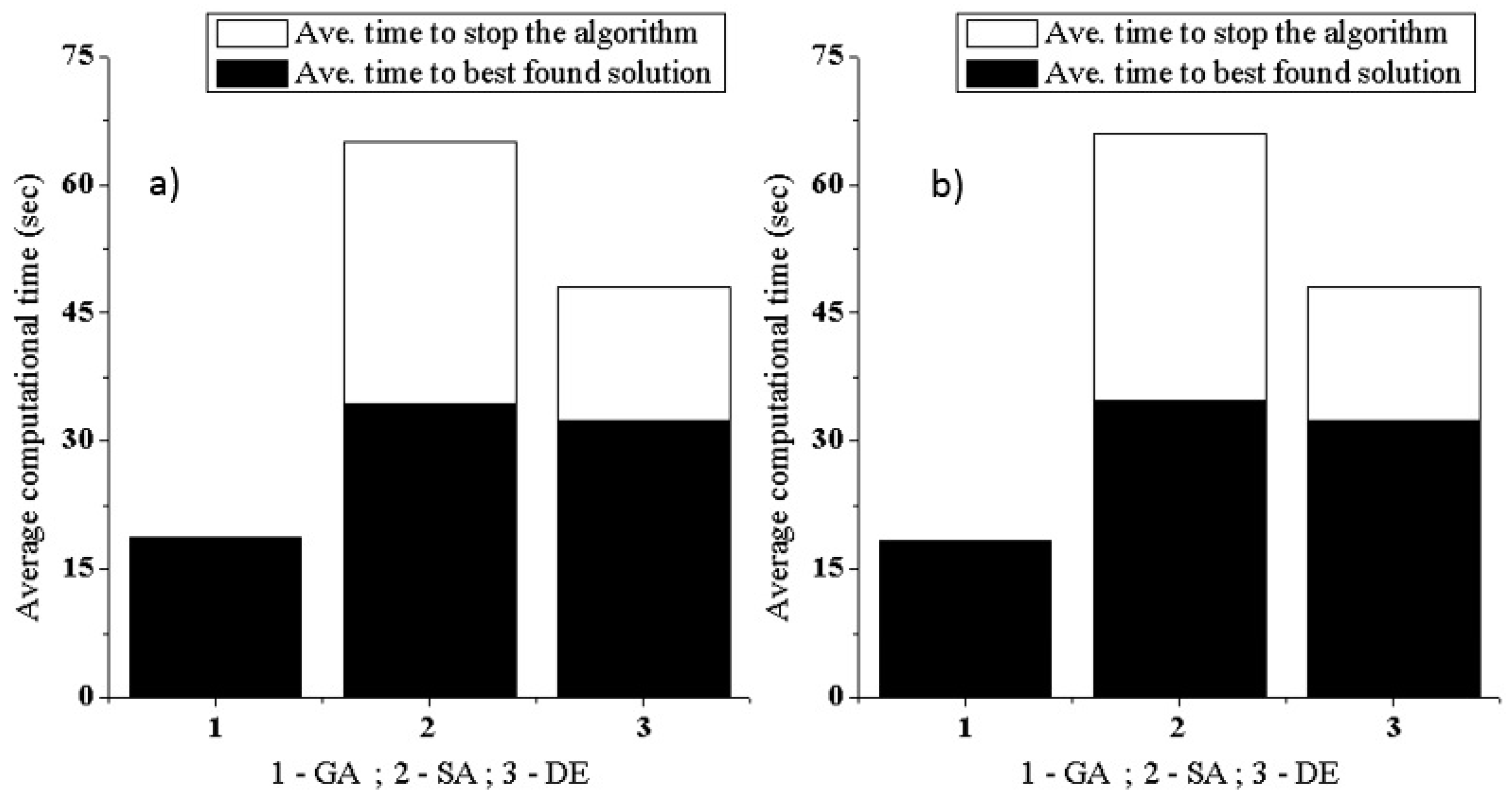
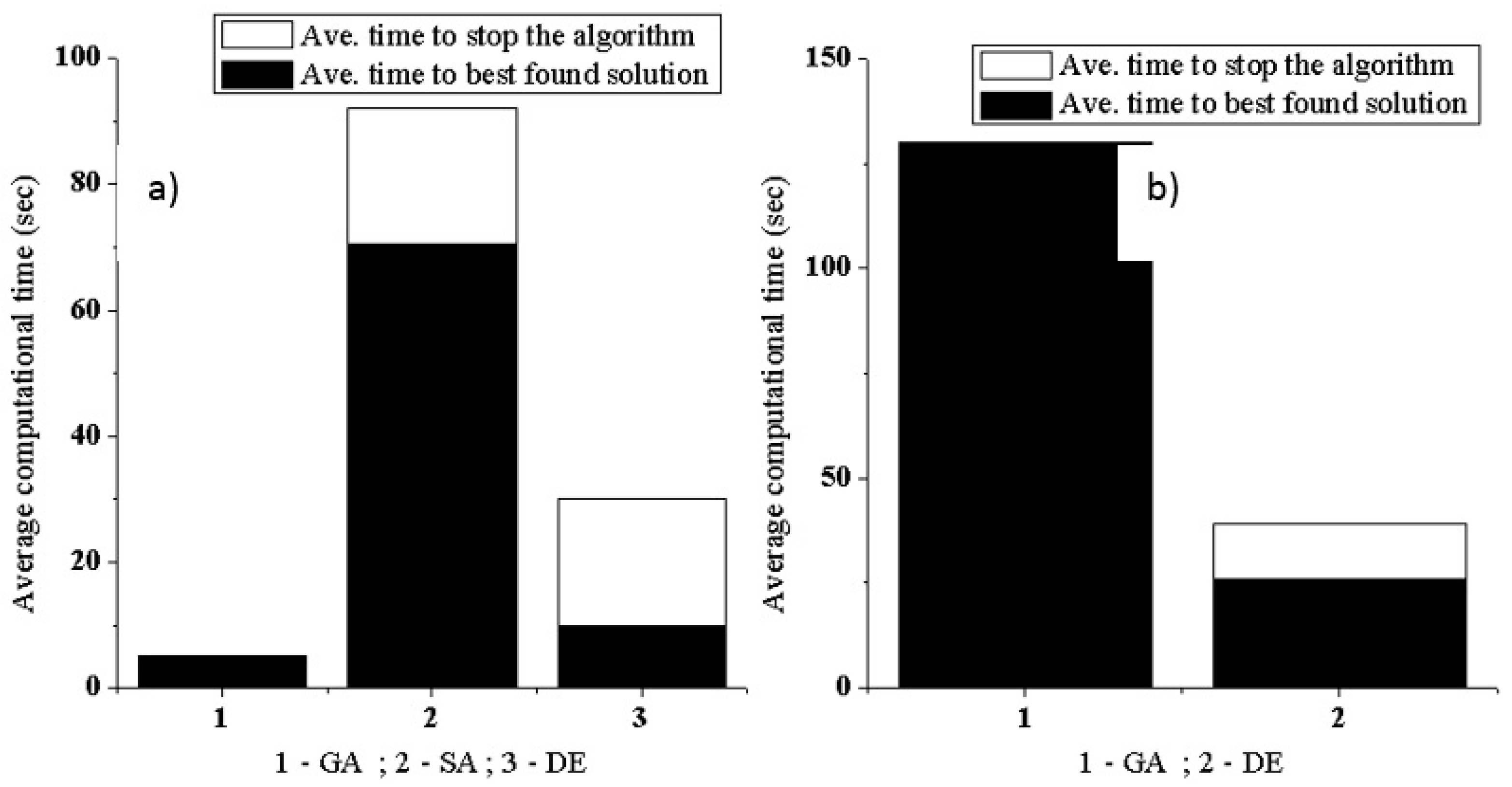
4.3. Computational Efficiency Test

Computational efficiency regarding the considered metaheuristic techniques is compared (evaluated) based on the real time calculation of the system running. Times for finding the best solution and the total running times which a complex heuristic is allowed to run just before the termination are reported.

In Test case-1, as shown in Figure 28a, the average total computational time of SA is 91.5 s. SA takes an average of 76 s for finding the best solution, or 83% of total time, and consumes 15.5 s to meet the stopping condition. For DE, the average total computational time of DE is 33 s, the average time to find the best solution is 11 s, or 3% of total time. In Test case-3, as can be seen in Figure 28b, DE achieves the same performance. The average total computational time of DE is 33 s. DE consumes 26 s, which is 78% of the average total time, is higher than Test case-1 to search the best solution because of taking more constraints than Test case-1. Performance of GA is weak, as the search takes few iterations, less than the average 5.03 s to meet the stopping condition for test case 1 and more than 130 s total computational time, but GA cannot achieve optimal findings like SA and DE.

In Test cases 4 and 5, as represented in Figure 29a,b, in both test cases the algorithms have the same average calculation time. SA consumes highest average total computational time, which is 66 s, DE takes 48 s to meet the stopping condition, but only 33 s which is approximately the same as SA for finding the best solution (50% of average total computational time). The computational time of the algorithms is controlled by a few key important parameters. For SA, it depends on how big the initial temperature T_o, the final stopping temperature T_min and the number of runs run_max with respect to every temperature’s value are. For DE, it depends on the total number of iterations i_max. The computational time also certainly depends on the configuration of the computer and the structure of the code. The computational time to find the best solution depends on how simple of the algorithm’s structure is and how good the parameter selections are. Therefore, choosing a good parameter setting is significantly important as it affects the time consumption and also the quality of the solutions.

4.4. Robustness Test

Robustness of a metaheuristic is evaluated (compared) by measuring the less sensitive capability against different types of applied system, and parameter tuning than other approaches [57]. A heuristic that can only get an excellent solution within only one instance of a problem or cannot perform well in reaching to the optimal finding when a small adjustment of a parameter setting is made is arguably not very interesting and also not robust. In Section 4.1, the SA and DE algorithms have been tested with five TEC model case studies, and the tests show that DE is more robust, performing well in all of the problems with one set of parameters and SA is less robust in terms of diverse instances of the problem. To give more justification of the robustness of the algorithms, eight sets of parameters of both algorithms are used based on small changes to the original set of parameters from Table 2 and Table 3. To test the robustness of the algorithms, Test cases 1, 2, 4 and 5 are used, the algorithms are run in 30 times and we collect the average value of best fitness, and also standard deviation.

Main parameters of DE which have the significant impact on its performance as well as its robustness are F, CR and P. The maximum number of iterations i_max does not affect the quality of the solution, and a large enough i_max can maintain the searching process for finding the optimal solution. For SA, the main parameters which impact its robustness are T_o, n_max, α, T_final. The original set of parameters for DE and SA are (F, CR, P) = (0.85, 0.95, 30) and (T_o, n_max, α, T_final) = (100, 300, 0.95, 10⁻¹⁰). The findings are shown in

Table 11. Obtained data after running TEC model with different sets of DE parameters.

No.	(F, CR, P)	Test Case-1	Test Case-3	Test Case-4	Test Case-5
		(Ave. Qc, Std Qc)	(Ave. Qc, Std Qc)	(Ave. Qc,c, Std Qc,c)	(Ave. COP, Std COP)
1	0.95, 0.95, 30	(7.421 W, 0)	(6.596 W, 0)	(3.105 W, 0)	(0.1677, 0)
2	1.0, 1.0, 35	(7.421 W, 0)	(6.596 W, 0)	(3.105 W, 0)	(0.1677, 0)
3	0.97, 0.97, 30	(7.421 W, 0)	(6.596 W, 0)	(3.105 W, 0)	(0.1677, 0)
4	0.93, 0.97, 27	(7.421 W, 0)	(6.596 W, 0)	(3.105 W, 0)	(0.1677, 0)
5	0.93, 0.93, 25	(7.421 W, 0)	(6.596 W, 0)	(3.105 W, 0)	(0.1677, 0)
6	0.91, 0.91, 23	(7.421 W, 0)	(6.596 W, 0)	(3.105 W, 0)	(0.1677, 0)
7	0.85, 0.9, 21	(7.421 W, 0)	(6.596 W, 0)	(2.720 W, 0.25)	(0.1377, 0.046)
8	0.80, 0.2, 19	(7.339 W, 0.10)	-	-	-
9	0.75, 0.18, 19	(6.981 W, 0.804)	-	-	-

and

Table 12. Obtained data after running TEC model with different set of SA parameters.

No.	(To, nmax, α, Tfinal)	Test Case 1	Test Case 4	Test Case 5
		(Ave. Qc, Std Qc)	(Ave. Qc, Std Qc)	(Ave. Qc, Std Qc)
1	(100, 300, 0.95, 10−10)	(7.417 W, 0.0025)	(3.105 W, 0)	(0.1677, 0)
2	(102, 310, 0.9, 10−10)	(6.918 W, 1.049)	(3.105 W, 0)	(0.1677, 0)
3	(98, 290, 0.9, 10−10)	(6.9015 W, 1.588)	(3.105 W, 0)	(0.1677, 0)
4	(96, 285, 0.85, 10−10)	(6.769 W, 1.465)	(3.105 W, 0)	(0.1677, 0)
5	(94, 280, 0.85, 10−9)	(6.68 W, 1.674)	(3.105 W, 0)	(0.1677, 0)
6	(92, 275, 0.8, 10−9)	(5.141 W, 2.342)	(3.105 W, 0)	(0.1677, 0)
7	(90, 270, 0.8, 10−8)	(6.277 W, 1.834)	(3.105 W, 0)	(0.1677, 0)
8	(88, 265, 0.75, 10−8)	(5.396 W, 2.451)	(3.105 W, 0)	(0.1677, 0)

.

As it can be seen in Table 11, DE achieves the same average value of best fitness with 0 value of standard deviation with the first five sets of parameters, meaning that for every test case, DE always obtains the optimal cooling rate or COP in every run. These findings show the strong robustness of DE. However, the robustness of DE is reduced in Test case-1 or even cannot find an optimal solution in Test cases 3, 4 and 5. That’s because the value of CR has been reduced a lot (from the range [0.9–1] to the range [0–0.2]), causing the slow convergence of the search process.

From Table 12, the stability of SA decreases in the second adjustment even keeping constant the final temperature T_final and the run_max. Reducing T_o and α or increasing T_final leads to a significant reduction of the number of iterations, and the algorithm meets the stopping condition before coming to convergence. Reducing run_max leads to a limitation of the number of random points generated with respect to every value of temperature. SA is less robust than DE considering the sensitivity to parameter adjustment.

4.5. Test on HSAGA and HSADE

As it can be seen within Sub-Section 4.1, SA was tested under non-linear constraint conditions in Test case-2, and cannot handle it. GA can solve constraint problems but has low performance in terms of stability. Hybridization of GA and SA can eliminate the defects of regarding both two methods, uncover their advantages, and eventually improve the efficiency of the solution process.

HSAGA is the combination of both algorithms, SA and GA. HSADE is the combination of SA and DE. The structure of these hybrid algorithms is heavier than that of the single ones and consumes more time to find the optimal solution. The parameter selection is also complicated and it will impact the robustness of the algorithm.

This test is used to evaluate the stability of the hybrid techniques. Test cases 1 and 3 are used to test the algorithm under non-linear inequality and non-linear equality constraint, respectively. Same conditions, i.e., running 30 trials, is used to measure the stability of the technique. All the necessary data are obtained and compared with the findings, which have been achieved of SA and DE from Table 8 and Table 9.

The findings of the hybrid techniques for Test case-1 and Test case-3 are shown in

Table 13. Obtained data after 30 trials running for Test cases 1 and 3 by using HSAGA.

Technique Used	HSAGA		HSADE
Test Case	(1) Qc (W)	(3) Qc (W)	(1) Qc (W)	(3) Qc (W)
Standard deviation	0.0269	0.5409	0	0
Average value of best fitness	7.38	5.916	7.421	6.596
Minimum value of best fitness	7.42	4.907	7.421	6.596
Maximum value of best fitness	7.33	6.95	7.421	6.596

. Obtained findings from HSAGA are slightly better than what are achieved from SA and GA. Standard deviation values measured by HSAGA approach are lower than SA and GA in Test cases 1 and 3, which means HSAGA are more stable and more effective to find optimal solution. However, these findings still not achieve as good findings as DE’s approach, hence, in finding part HSAGA is not used.

Obtained findings from HSADE are like those obtained by the DE method and definitely better than GA and SA. Standard deviation values measured by the HSADE approach are also 0 like with DE. The addition of DE to the hybrid of SA and DE empowers the performance of the hybrid technique, but cannot get better values of the objective function. This test proves that DE has the best performance among SA, hybrid HSAGA, HSADE in solving a diversity of test cases.

4.6. Optimization Results

Thanks to the process of evaluating (comparing) the performances of the metaheuristic algorithms: SA and DE, findings from optimizing the design of STEC and TTEC are obtained. Some case studies preferred from the works of [29,30] are presented as follows:

▪

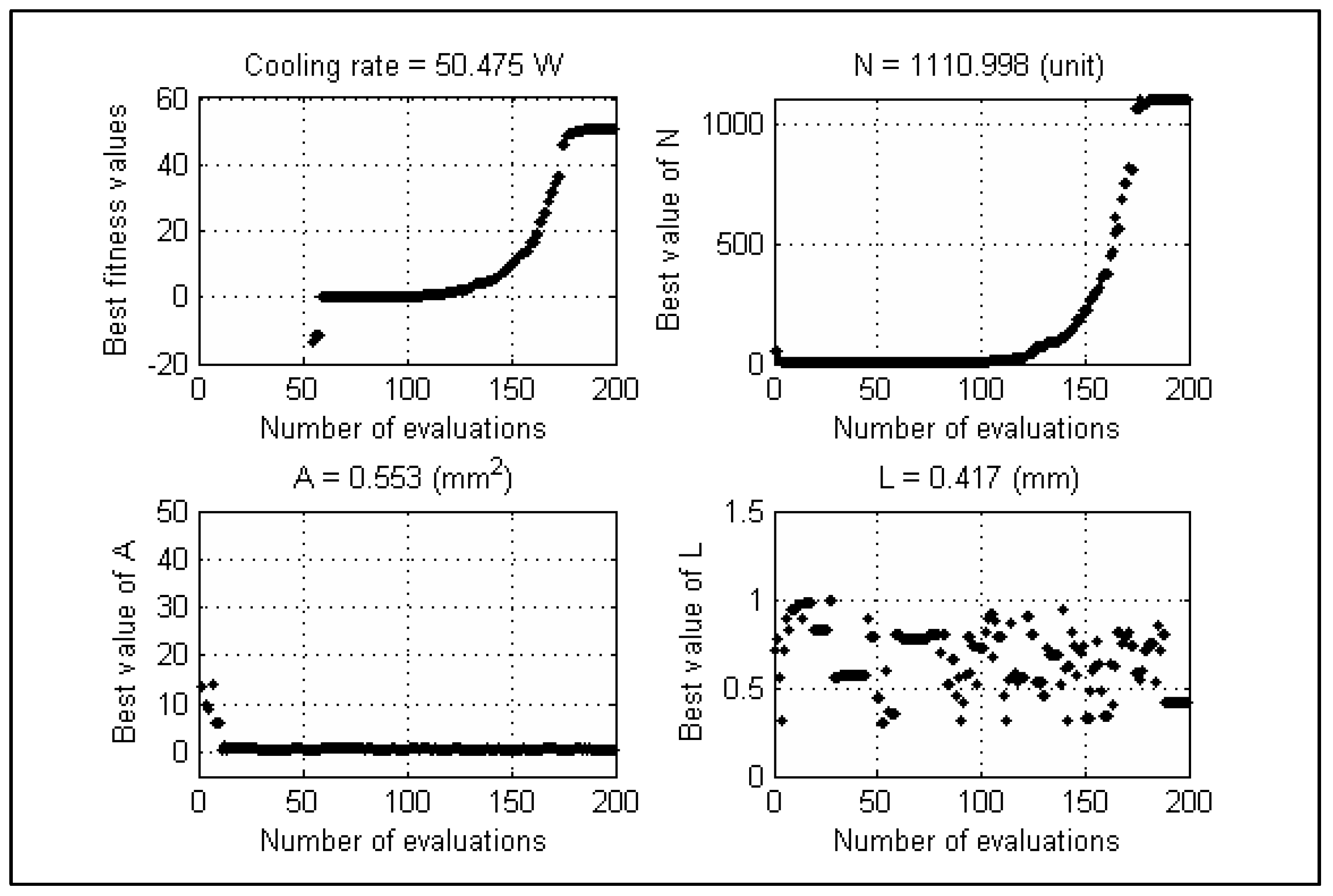
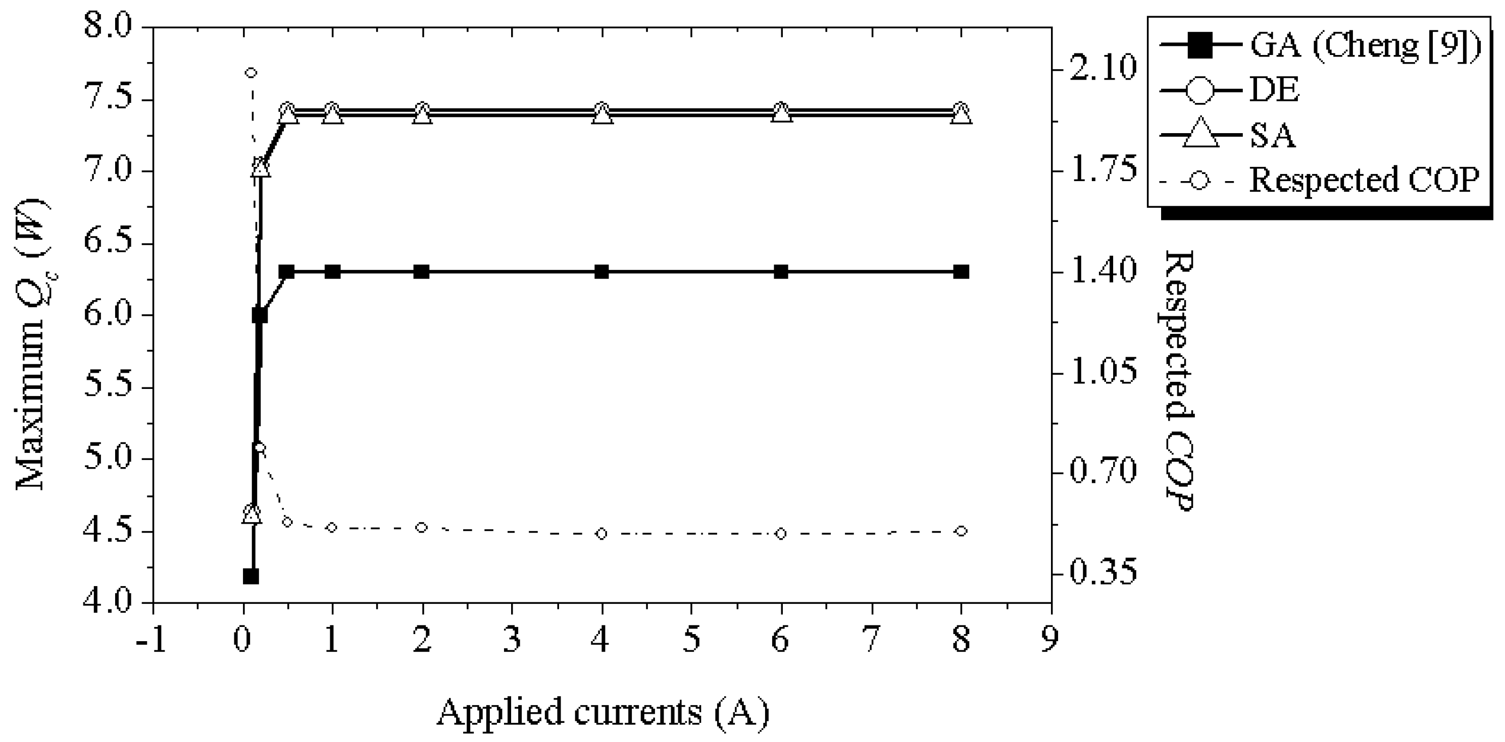
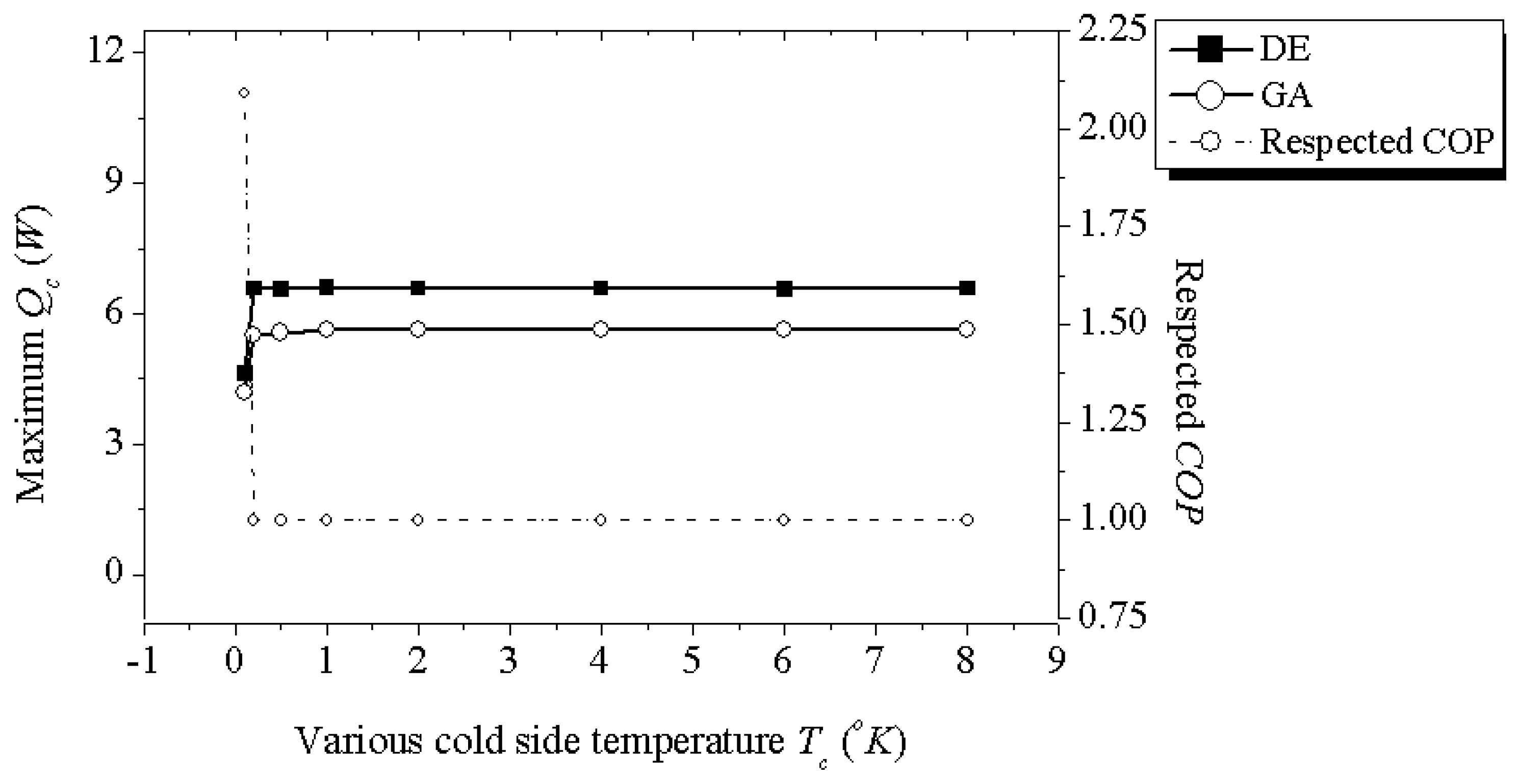
Case-1: The parameter settings of the STEC model follow Table 6 and SA and DE are applied to find an optimal STEC geometric design under the limitation of total area S = 100 mm² and the maximum cost for material is $385. However, the applied current is varied from 0.1 A to 8 A, hot side and cold side temperature are set as T_h = T_c = 323 °K, the requirement of COP is neglected. With ΔT = 0 °K, the maximum cooling rate for every specific value of applied DC current can be achieved. Because COP is not considered, SA can provide good performance and is run under the same conditions, and the results from the Cheng’s work employing GA are used for the comparison.

▪

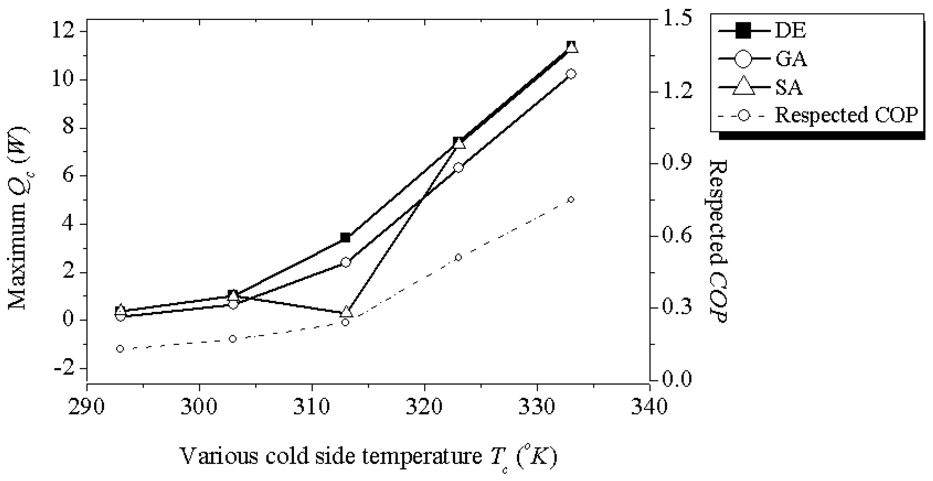
Case-2: Same condition settings as Case-1 but with the cold side temperature T_c is varied from 283 °K to 323 °K and hot side temperature T_h still remains in 323 °K and the applied current is kept in 1 A. The obtained results are useful for designers to choose a suitable STEC geometric design which yields enough cooling capacity and satisfies the required temperature difference ΔT with a defined input current.

▪

Case-3: Same condition settings as Case-1. In this case, COP is not considered as a requirement though it has an important role in STEC performance. Considering cooling rate as an objective function which is single-objective optimization, in this case, the requirement of COP is required as a constraint condition which has a value equal to 1.

▪

Case-4: In this study, the parameters settings of TTEC follows Table 7 but the total number of semiconductor elements N is changed to 200 to compare with the results of Cheng [29]. The first type of TTEC as connected electrically in series (I_h = I_c) and second type of TTEC is separated electrically in series (I_h ≠ I_c) are used, T_c,c is varied from 210 °K to 230 °K and T_c,h is kept in 240 °K.

▪

Case-5: In this case, the effect of contact and spreading resistance are taken into consideration. The parameter settings of two types of TTEC follow

Table 14. Parameter setting of TTEC considering the effect of total thermal resistance RS_t.

No.	Parameters	Description
1	Objective function	Case 5: Single-obj. opt.—Maximize Qc,c or maximize COP.
		Case 6: Multi-obj. opt.—Maximize Qc,c and COP
2	Variables	Ic—Input current to the cold stage TTEC (A)
		Ih—Input current to the hot stage TTEC (A)
		r—ratio number for TE modules between the hot stages and the cold stage (unitless)
3	Fixed variable	Nt = 100 (unit)
		G = 0.0018 (m)
		RSj = 0.02; 0.2; 2 (cm2K/W)
		Sh,s = 0.1 (cm)
		a = 0.02 (cm2)
		kh,s = 0.3 (W/cmK)
		Th,h = 300 (°K)
		Tc,c = 210 °K, 220 °K, 230 °K, 240 °K
4	Boundary constraint	4 (A) ≤ Ih ≤ 11 (A)
		4 (A) ≤ Ic ≤ 11 (A)
		2 ≤ r ≤ 7.33

and the calculations from Section 3.2.3, which are preferred from Rao [33] and Cheng’s work [30] with the consideration of contact and spreading thermal resistance. TTEC is used to produce temperature T_c,c = 210 °K at a temperature of T_h,h = 300 °K is needed to be optimized for maximizing Q_c,c and COP separately. The total number of semiconductor elements of TTEC is N_t = 100 units and the ratio of cross-sectional area to the semiconductor element is G = 0.0018. Thermal resistance is presented at the interface of TEC. Alumina with a thermal conductivity k_h,s equal to 30 W/m°K is a substrate for considering the spreading resistance. The thickness of the substrate S_h,s is equal to 0.1 cm. In order to consider the contact resistance, which is between the two stages, the joint resistance RS_j is varied from 0.02 to 2 cm²K/W.

▪

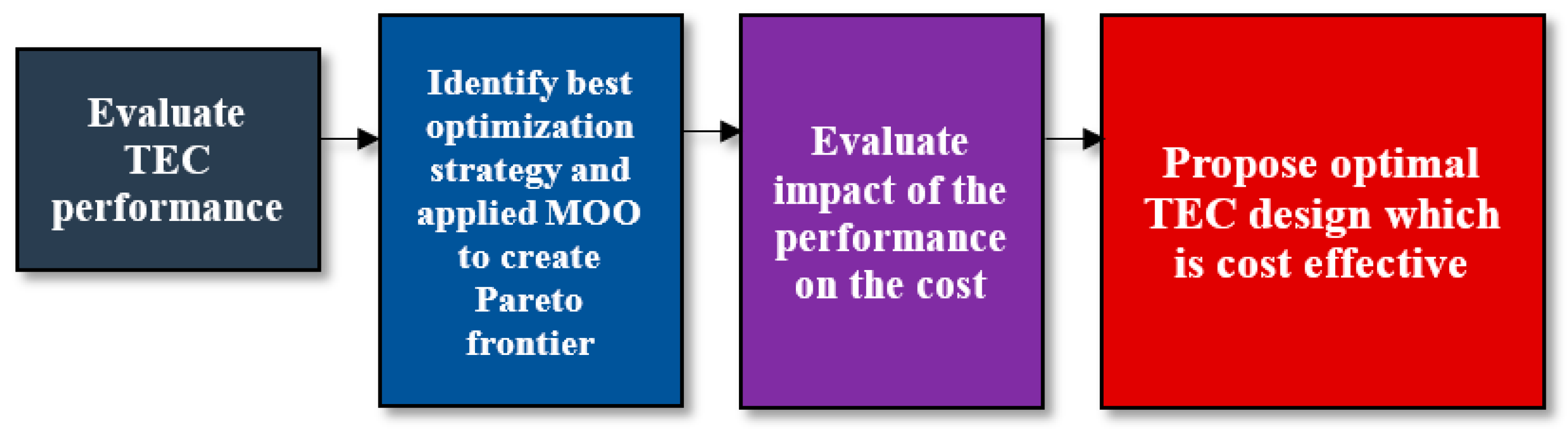
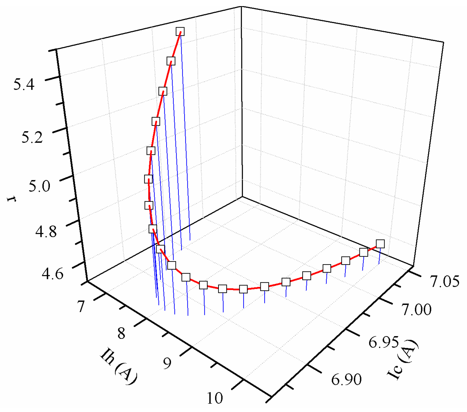
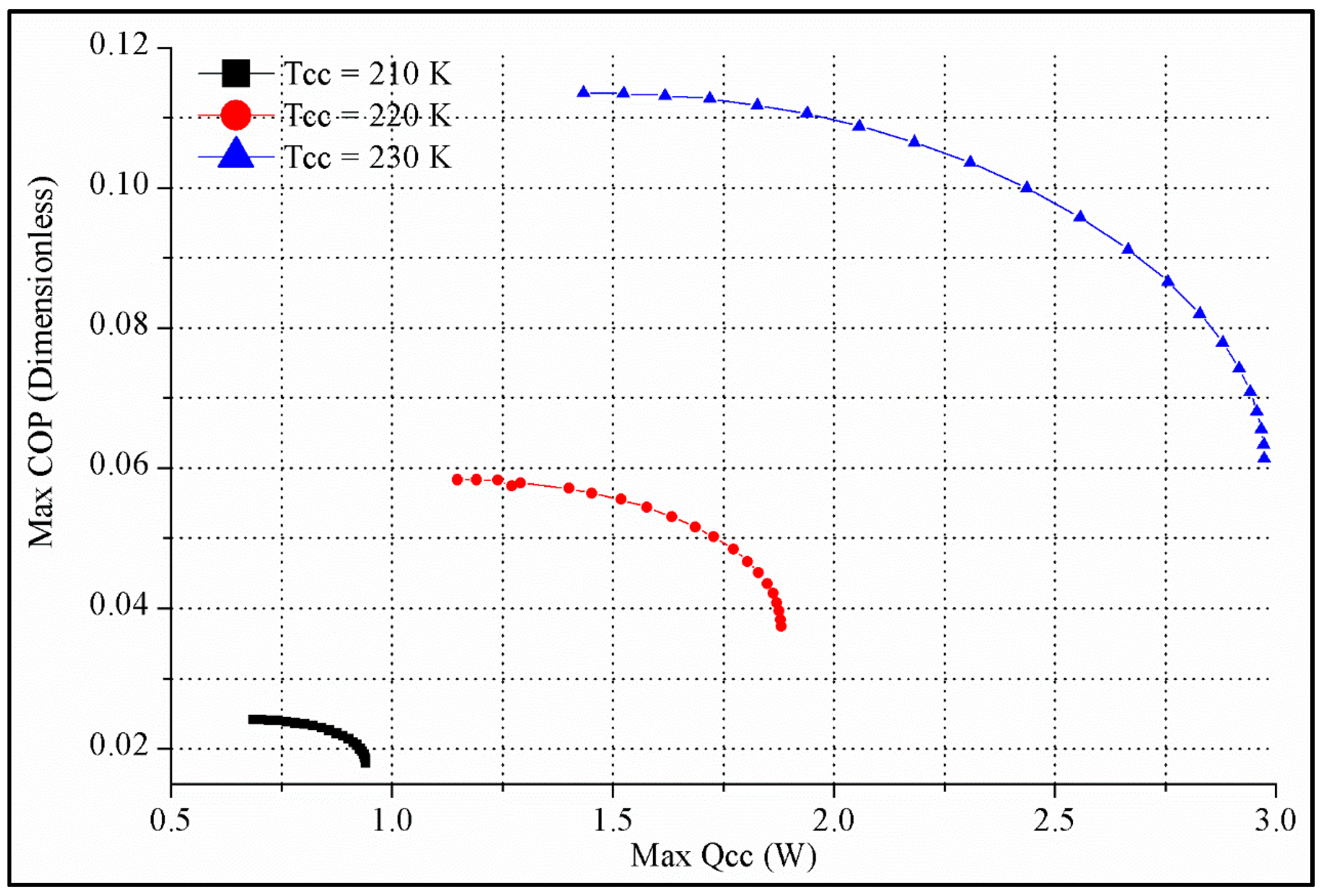
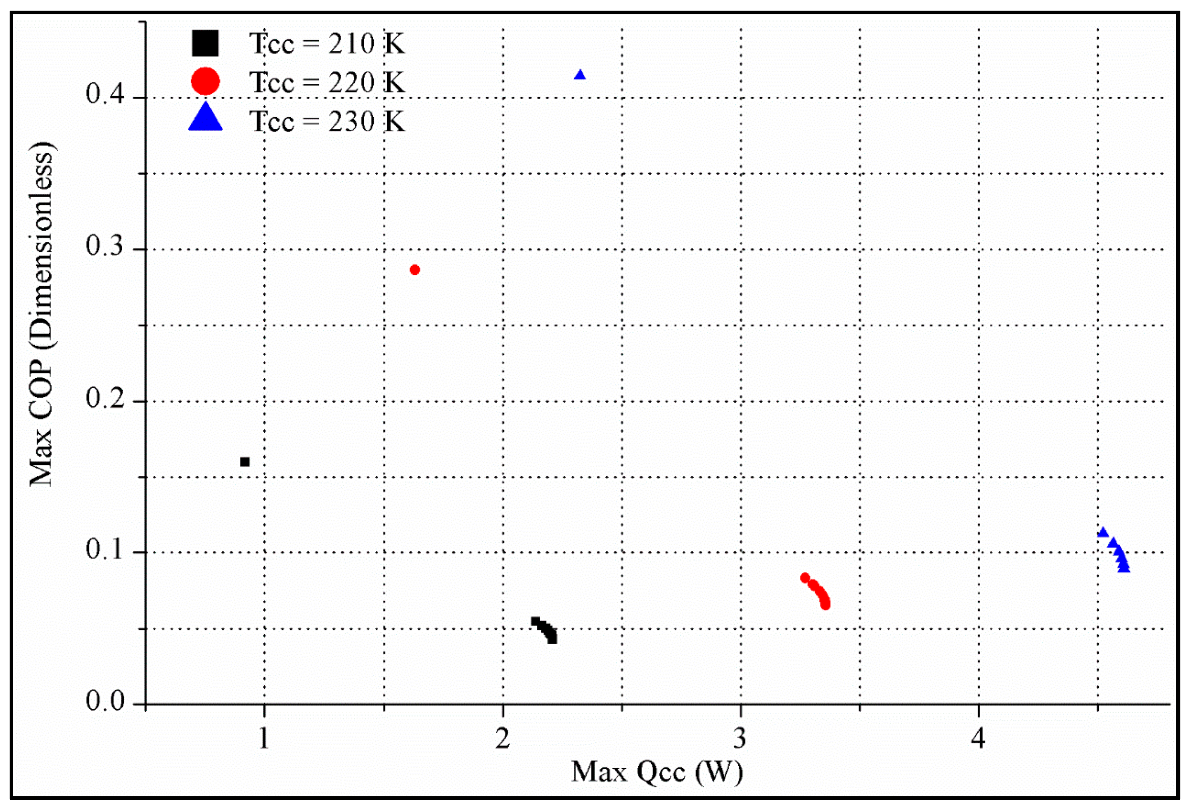
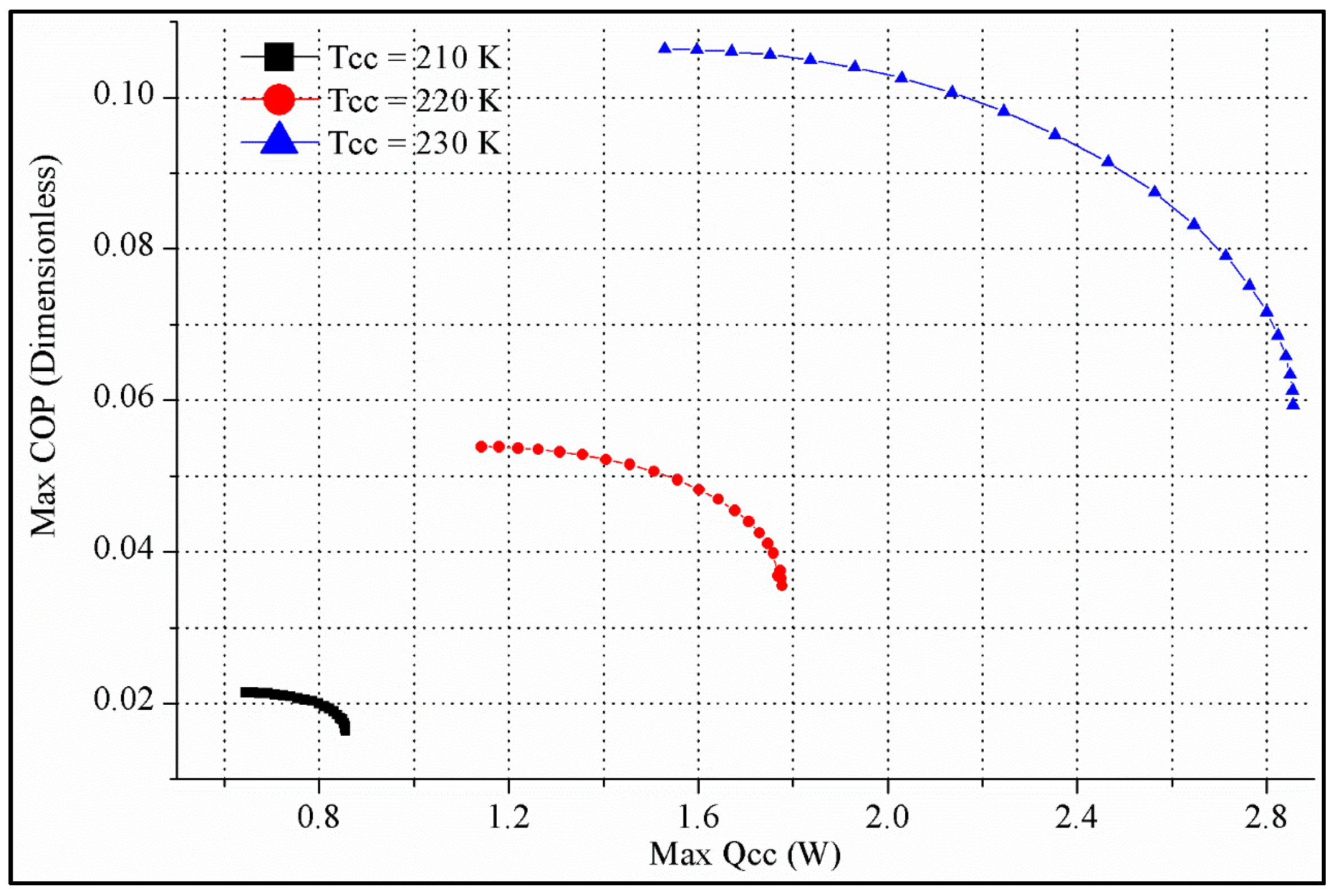
Case-6: In this case, multi-objective optimization maximizing Q_c,c and COP simultaneously to create the Pareto frontier. Following the parameter settings of Table 14, the TTEC type with better performance from Case-5 is chosen to form the Pareto front graph. TTEC designs with the balance of maximum Q_c,c and maximum COP are suggested.

4.6.1. Single-Objective Optimization Results

For the Case-1,

Table 15. Case-1: Obtained data after applying SA and DE for STEC model according to various input currents.

I (A)	DE				SA				COP
	Qc (W)	N (unit)	A (mm2)	L (mm)	Qc (W)	N (unit)	A (mm2)	L (mm)
0.1	4.63	842	0.09	0.3	4.63	841	0.09	0.3	2.09
0.2	7.04	842	0.09	0.3	7.04	841	0.09	0.3	0.79
0.5	7.42	437	0.17	0.3	7.42	437	0.17	0.3	0.5
1	7.42	217	0.35	0.3	7.42	221	0.34	0.3	0.51
2	7.42	108	0.7	0.3	7.42	108	0.7	0.3	0.51
4	7.42	55	1.39	0.3	7.42	55	1.39	0.3	0.49
6	7.42	36	2.09	0.3	7.41	36	2.08	0.3	0.49
8	7.42	27	2.82	0.3	7.42	27	2.82	0.3	0.5

represents the optimal parameters of design for STEC model over various applied currents from 0.1 A to 8 A obtained by applying DE and SA algorithms. The comparison with the work of Cheng using GA [29] is shown in Figure 30.

When the value of the optimal cooling rate is increased, the cross-sectional area regarding the semiconductor elements increases A and number of semiconductor elements N decreases, the length L doesn’t change during the search and reaches to the lower bound with the limit of 0.3 mm. As represented in Figure 30, when the input current is larger than 0.5 A, the maximum values regarding cooling rate obtained by SA and DE are approximately 7.42 W (which is seen as unchanged). The results demonstrate that STEC using SA and DE can reach its maximum capacity of cooling even in the context of various input currents. Moreover, these obtained results from DE and SA are about 17.8% higher than the obtained findings (results) in [29] by using GA with the same results obtained by SA. The figure points to better performance by SA and DE as compared to GA, which was used by Cheng [29]. With the same obtained design parameters from both the SA and DE algorithms, the respective COPs are calculated and they have the same value which is approximately 0.5. With various input currents and fixed temperature differences, Q_c increases while COP decreases and reaches a fixed value of 0.5. From there, the electrical power consumption of STEC for every optimal design parameters is also kept at a constant value of 14.84 W based on Equation (4) provided before.

Related to Case-2,

Table 16. Case-2: Obtained data after running SA and DE over various cold side temperature.

Tc (°K)	DE				SA				COP
	Qc (W)	N (unit)	A (mm2)	L (mm)	Qc (W)	N (unit)	A (mm2)	L (mm)
283	-	-	-	-	-	-	-	-	-
293	0.37	45	0.51	1	0.37	45	0.51	1	0.13
303	1.03	82	0.44	0.62	1.02	77	0.45	0.66	0.17
313	3.42	209	0.36	0.3	0.30	44	0.13	0.7	0.24
323	7.42	221	0.34	0.3	7.42	221	0.34	0.30	0.51
333	11.38	226	0.335	0.3	11.38	226	0.33	0.30	0.75

presents the optimal parameters of design for STEC model over various cold side temperature from 283 °K to 333 °K. As it can be seen from the table the optimal value of Q_c increases when the cold side temperature T_c is increased. The increase of Q_c is more obvious when T_c is above the hot side temperature T_h. Also, as T_c is increased, the optimal cross- sectional area of the semiconductor elements decreases as the number of semiconductor elements increases. Here, their length reaches a lower bound of 0.3 mm in order to achieve a the maximum Q_c.

Figure 31 presents the effects of optimal dimensions for maximizing Q_c, considering various T_c. As can be seen, the optimal Q_c increases together with T_c and if the value of T_c is increased more than 333 °K, the optimal Q_c also keeps increasing. At this point, the results obtained with DE are slightly better than the ones in the Cheng’s work [29], and not quite different from the ones obtained with SA. SA even performs worse than DE when T_c = 313 °K which yields a cooling rate 0.3 W, 11.4 times less than the DE approach. Because SA is less stable than DE, hence, in few running times, SA can find optimal cooling rate as good as using DE’s approach. Respective COP is calculated based on the obtained design parameters from DE approach. As it can be seen from Figure 32, with various cold side temperature, COP increases simultaneously with Q_c. This data show that when we want to design STEC, which yield a larger temperature difference ΔT with a fixed applied current and fixed volume, Q_c and the COP are decreased.

In the context of Case-3,

Table 17. Case-3: Obtained data after running DE in the context of various applied currents with the requirement of COP = 1.

I (A)	DE				COP
	Qc (W)	N (unit)	A (mm2)	L (mm)
0.1	4.63	842	0.09	0.3	2.09
0.2	6.59	723	0.1	0.3	1
0.5	6.59	288	0.26	0.3	1
1	6.59	145	0.52	0.3	1
2	6.59	72	1.04	0.3	1
4	6.59	36	2.09	0.3	1
6	6.59	24	3.15	0.3	1
8	6.59	19	4.18	0.3	1

presents the optimal design parameters for a STEC model in the context of various input currents along with the requirement of COP = 1. Briefly, SA cannot realize the system under the constraint of nonlinear equality. On the other hand, DE is able to show a good advantage, which is the ability to solve the problem with the constraint of nonlinear equality. Using DE, the achieved cooling rate reaches a value of 6.59 W, 17.3% higher than the results in Cheng’s work in which GA is employed. Moving to Figure 32, it can be verified that the DE is often better than GA. In the context of Table 17, the leg area should be increased for tolerating an input current which is higher.

For the Case-4,

Table 18. Case-4: Optima solutions of first type TTEC under various T_c,c.

First Type TTEC	Optimal Design Variables				DE and SA	GA— [29]
Tc,c (°K)	Nc	Nh	Ic (A)	Ih (A)	Max. Qc,c (W)	Max. Qc,c (W)
230	44	156	7.487	7.487	4.25	4.25
220	36	164	7.719	7.719	2.49	2.49
210	25	175	8.028	8.028	1.07	1.07
Tc,c (°K)	Nc	Nh	Ic (A)	Ih (A)	Max. COP	Max. COP
230	50	150	4.908	4.908	0.1	0.1
220	39	171	5.587	5.587	0.044	0.04
210	26	173	6.886	6.886	0.02	0.02

and

Table 19. Case-4: Optima solutions of second type TTEC under various T_c,c.

Second Type TTEC	Optimal Design Variables				DE and SA	GA— [29]
Tc,c (°K)	Nc	Nh	Ic (A)	Ih (A)	Max. Qc,c (W)	Max. Qc,c (W)
230	60	140	5.439	9.957	5.18	5.16
220	48	152	5.874	9.925	3.09	3.07
210	33	167	6.508	9.883	1.36	1.35
Tc,c (°K)	Nc	Nh	Ic (A)	Ih (A)	Max. COP	Max. COP
230	55	145	4.619	5.212	0.09	0.09
220	56	144	5.459	6.286	0.05	0.04
210	30	170	6.358	7.479	0.02	0.02

show the optimized parameters by using DE and SA for maximizing the cooling rate Q_c,c as well as maximizing COP when the first type TTEC and second type TTEC are considered and the comparison with the optimized parameters as provided in Cheng’s work [29] employing the GA approach. As it can be understood, when T_c,c is increased, it means that the temperature difference between the temperature of the cold side of the cold stage and the temperature of the hot side of the hot stage ΔT becomes smaller, and the optimal value of the maximum cooling rate and maximum COP increase. These results demonstrate that the second type of TTEC has better performance for the maximum cooling capacity than the first type TTEC. In some applications, in which cooling capacity is more important, a second type TTEC will produce better performance. When comparing the obtained results between the meta-heuristics, DE and SA obtained same output and they seem to perform better than GA in every value of T_c,c. With the first type TTEC, there is no difference between the optimal results. With the second type TTEC, when T_c,c is from 210 °K to 230 °K, the present approach using DE increases the cooling capacity by 0.74%, 0.65% and 0.39% when compared with the GA approach used by Cheng’s work [29]. Similarly, for the maximum COP, the present approach provides 25% higher COP when compared with the GA approach (as the T_c,c = 220 °K).

Related to Case-5, the optimized parameters for the first type TTEC and second type TTEC are shown in

Table 20. Case-5: Optima solutions of first type TTEC under different values of RS_j.

First Type TTEC	Optimal Design Variables				DE and SA	GA— [30]
RSj (cm2K/W)	Nc	Nh	Ic (A)	Ih (A)	Max. Qc,c (W)	Max. Qc,c (W)
0.02	14	86	8.266	8.266	0.723	0.73
0.2	14	86	8.395	8.395	0.816	0.818
2	19	81	9.883	9.883	2.185	2.123
RSj (cm2K/W)	Nc	Nh	Ic (A)	Ih (A)	Max. COP	Max. COP
0.02	15	85	6.920	6.920	0.021	0.019
0.2	16	84	6.934	6.934	0.024	0.020
2	21	79	7.086	7.086	0.064	0.048

and

Table 21. Case-5: Optima solutions of second type TTEC under different values of RS_j.

Second Type TTEC	Optimal Design Variables				DE and SA	GA— [30]
RSj (cm2K/W)	Nc	Nh	Ic (A)	Ih (A)	Max. Qc,c (W)	Max. Qc,c (W)
0.02	21	79	6.864	9.967	0.856	0.755
0.2	18	82	7.043	10.004	0.940	0.838
2	20	80	9.311	10.510	2.210	2.103
RSj (cm2K/W)	Nc	Nh	Ic (A)	Ih (A)	Max. COP	Max. COP
0.02	16	84	6.740	7.121	0.021	0.019
0.2	15	85	6.962	6.901	0.024	0.021
2	12	88	11	4	0.160	0.061

with the consideration of total thermal resistance RS_t, respectively. As can be seen, the maximum cooling capacity and maximum COP performance are improved and more obvious when the joint resistance is increased. When comparing the obtained results using DE with the GA approach of Cheng, in terms of maximum COP, DE and SA totally perform better than GA in terms of maximum Q_c,c. DE and SA can properly maintain and improve the performance. The improvement of the optimal results using the DE and SA approaches compared to the GA approach will become more significant when the total number of thermo-elements or cold temperature on the cold side are increased as in Case-1 when compared to the optimal results regarding Case-1 and Case-2. In the same condition which means T_c,c is equal to 210 °K and total number of thermal element is 100, can see that the optimal results of the two case studies are similar. This means that the optimization technique has the ability to neglect the effect of contact and thermal spreading resistances.

4.6.2. Multi-Objective Optimization Results

In the context of Case-6, second type TTEC with better performance was chosen to test the multi-objective optimization, RS_j was varied from 0.2 to 2 cm²K/W, and to give more diverse results, T_c,c was varied from 210 °K to 230 °K in every value of RS_j. After the Figure 33 showing 3D distribution of Pareto optima variables, Figure 34, Figure 35 and Figure 36 show the Pareto frontier of multi-objective optimization on cooling rate and COP when considering a second type TTEC. The Pareto-front briefly separates the space of objective function into two parts: the part below the curve includes non-optimal solutions and the part above includes in feasible solutions. Figure 33 shows the 3D graph of the optimal variables with respect to the Pareto front in Figure 34. As it is represented in Figure 34, the extreme values regarding cooling rate, and COP are (0.6457 W; 0.8555 W) and (0.0214; 0.0164) at RS_j = 0.02 cm²K/W and T_c,c = 210 °K are same as the ones within single-objective optimization problems considered earlier in Case 5. With a specific value of RS_j, when T_c,c is varied from 210 °K to 230 °K, the achieved Pareto frontier spreads higher than previously. That means the optimal values which are cooling rate and COP increase obviously when the temperature difference becomes smaller (T_c,c is increased). The ratio between the optimal values which respect to the increasing of T_c,c ranges from 1.52 to 2.43.

Table 22. Obtained optima solution of TTEC for multi-objective optimization.

Second Type TTEC	w1	Ih (A)	Ic (A)	r	Max. Qc,c	Max. COP
RSj = 0.02 cm2K/W Tc,c = 210 °K	0	7.1213	6.7396	5.3969	0.6457	0.0214
	0.5	8.5062	6.7056	4.7398	0.799	0.02
	1	9.9673	6.8638	4.6913	0.8555	0.0164
RSj = 0.02 cm2K/W Tc,c = 220 °K	0	5.8037	5.9636	3.8962	1.1424	0.0538
	0.5	7.8384	5.8902	3.0916	1.6011	0.0482
	1	10.011	6.2804	3.1262	1.7767	0.0355
RSj = 0.02 cm2K/W Tc,c = 230 °K	0	4.5574	5.296	3.3146	1.5295	0.1064
	0.5	7.1472	5.1585	2.294	2.4651	0.0915
	1	10.0444	5.8688	2.4079	2.8554	0.0594
RSj = 0.2 cm2K/W Tc,c = 210 °K	0	6.9015	6.9622	5.4852	0.6865	0.0241
	0.5	8.4447	6.8835	4.6794	0.8744	0.0222
	1	10.0038	7.0427	4.6041	0.94	0.018
RSj = 0.2 cm2K/W Tc,c = 220 °K	0	5.5202	6.2531	4.1809	1.148	0.0583
	0.5	7.7598	6.0721	3.1288	1.6855	0.0516
	1	10.0486	6.4637	3.1317	1.8805	0.0374
RSj = 0.2 cm2K/W Tc,c = 230 °K	0	4.1216	5.7414	3.9161	1.4334	0.1136
	0.5	7.0816	5.3424	2.3521	2.5569	0.0958
	1	10.0835	6.0516	2.434	2.973	0.0614
RSj = 2 cm2K/W Tc,c = 210 °K	0	4	11	7.33	0.9207	0.1596
	0.5	4	11	7.33	0.9207	0.1596
	1	10.5099	9.3109	3.9839	2.2097	0.0429
RSj = 2 cm2K/W Tc,c = 220 °K	0	4	11	7.33	1.6316	0.2866
	0.5	4	11	7.33	1.6316	0.2866
	1	10.5716	8.7926	3.1648	3.3572	0.0651
RSj = 2 cm2K/W Tc,c = 230 °K	0	4	11	7.33	2.3244	0.4142
	0.5	4	11	7.33	2.3244	0.4142
	1	10.6264	8.3924	2.6641	4.6084	0.0897

collects some outstanding data which have detailed information on optimal design variables, the optimal values of cooling rate and COP obtained from the multi-objective optimization process. The maximum cooling capacity observed at w₁ equal to 1 where the COP is minimized. The maximum COP occurs at w₁ equal to 0 as the cooling capacity has the minimum value at this point. When w₁ is equal to 0.5, the maximum of cooling capacity is considered as important as maximum COP. These data are more for designers to refer to and choose the suitable parameters of I_h, I_c and r flexibly so that they can satisfy the condition of both objectives based on the demand of practical applications.

5. Discussion

The optimization models of STEC and TTEC considering cooling rate and COP as two objective functions are presented. Our parameter selection of TEC models including STEC and TTEC follow the works of Cheng [29,30] and Rao [33], respectively, for more convenience in comparison between the obtained results. Testing experiments are done to evaluate the performance shown by the algorithms, considering some predefined criteria such as convergence speed, computational effort, stability and robustness test with some predefined test cases.

The 2D and 3D convergence curve of each algorithm is analyzed and discussed with respect to its computational time. The stability and computational efficiency are investigated by running the algorithm over 30 trials, then calculating the average value, standard deviation value and average time consumed of the best fitness for comparison purposes. With the capability of solving the diverse problems such as equality, inequality constraint handling and also the less sensitivity of algorithms to parameter setting changes, the robustness is then evaluated.

DE can yield the best optimal results with the least computation time among the optimization techniques during the first time the system is run, and retains the highest performance with 0 standard deviation during the remaining running time. It shows reliability, reliability and robustness combined with computational efficiency.

HSAGA was suggested to overcome the weaknesses of the SA and GA such as capability of handling non-linear equality constraints and the poor stability, respectively. HSAGA has shown better performance better than SA and GA but worse than DE despite having a heavier structure and consuming more time to find an optimum solution. HSADE obtained the same performance as DE and consumed more computational time to find the best fitness function.

Findings from optimizing STEC and TTEC were conducted by using SA and DE and applied in defining case studies. Single-objective optimization is applied for STEC with the cooling rate as an objective function and multi-objective optimization is applied for TTEC, considering the cooling rate and COP are to be optimized simultaneously by using a weighted method. With this simulation strategy, better design parameters of both types of TEC have been achieved. In case study 1, with the geometric design X₁ = (N, A, L)₁ = (437, 0.17, 0.3) and applied current 0.5 A is enough to produce maximum cooling rate 7.42 W with COP equal to 0.5 and temperature difference ΔT = 0 °K. In case studies 2, 4 and 5, depending on the desire temperature difference, a suitable set of design parameters for the TEC can be chosen to yield a large enough cooling rate with a corresponding high COP. In case study 3, with geometric design X₂ = (N, A, L)₂ = (723, 0.1, 0.3) and applied current 0.2 A is enough to produce a maximum cooling rate 6.59 W with a COP equal to 1 and temperature difference ΔT = 0 °K. In case study 6, with multi-objective optimization, the Pareto front has balanced the importance of maximum cooling rate and maximum COP and is significant for designers to choose a suitable design in practical applications.

In addition to the explanations above, some important remarks from the performed tests (applications) can be expressed briefly as follows in order to inform readers about what has been accomplished with this study and what can be done in similar future applications starting from the results presented here:

▪

Results provided here are some proofs of the success of SA and DE in solving single-objective and multi-objective optimization problems.

▪

Results of this study contribute to the previous findings in the literature (and also ideas in this study) regarding the better optimization performance of both SA and DE than GA.

▪

The study here provided a wide examination of the optimization problems of TECs by focusing on the stability, reliability, robustness and computational efficiency of the techniques used. These are important to have accurate ideas about also the success of SA and DE according to objective tests—problems and performance of the GA.

▪

According to the obtained findings (results), it is possible to indicate that the objectives of the study have been met. In detail, our investigation on using metaheuristic stand-alone techniques like SA and DE for STECs and TTECs has been successful. Following that, the research has proven that the development of hybrid techniques for STECs and TTECs has resulted in positive findings. Finally, validation of all the techniques used (stand-alone and hybrid ones) on STECs and TTECs has been done through the explained methodology—research process.

▪

Multi-objective optimization approaches discussed in this study are useful for the designer to find the suitable design parameters of TECs balancing the important role of cooling rate and COP.

▪

For the interested readers, the results reported here open doors to further investigations of STECs and TTECs using additional alternative metaheuristic and stand-alone techniques, and also alternative methods for them. Additionally, it is good to run alternative design optimizations by using the same SA and DE stand-alone techniques and also hybrid techniques developed with them.

▪

Optimization is a process occurring in life itself and especially hard problems require the use of effective and accurate techniques to obtain the desired optimal results. Currently, metaheuristic techniques are important ways to deal with such problems. There are many unsolved hard problems or problems requiring better solution methods waiting for researchers to perform the necessary investigations on them.

6. Conclusions and Future Work

In this study, Differential Evolution (DE) and Simulated Annealing (SA) and hybrid algorithms were used and applied successfully in two different types of TEC model which are single-stage TEC and two-stage TEC to find their optimal design parameters. In single-stage TECs, the design parameters are the geometric parameters of the semiconductor element, like the length and also the area of the semiconductor column, and the total number of semiconductor elements in the single-stage TEC. In a two stage TEC, the design parameters are the applied current within the hot stage and also the cold stage, and number of total semiconductor elements of two stage TEC. Cooling rate and COP are criteria which are remarkable for evaluating the performance shown by STECs. They are considered as objective functions and optimized separately or simultaneously by using a weighted method. For single-objective optimization, the cooling rate is more the focus than COP, the COP is neglected or also can be accepted as a satisfied condition (COP = 1) to obtain the optimal cooling rate value. Both DE and SA are tested in some defined test cases of STECs and TTECs with consideration of constraint conditions. Another technique, Genetic Algorithm (GA), is used for comparison to evaluate their performance. Parameter settings of the TEC model are referred from the research of Cheng for a single-stage TEC model and the research of Cheng and Rao for a two-stage TEC model. Parameter settings of the algorithms are referred from the literature review, which represents a combination of the authors’ experience when working with MATLAB.

According to the performed tests (applications), both considered algorithms show more stability and reliability than GA. SA can perform well with unconstrained and non-linear inequality constraints. For non-linear equality constraint conditions (COP = 1), SA cannot solve the problem. DE has the capability to handle all the test problems of TECs, including problems with non-linear inequality and equality constraint (COP = 1) and shows perfect stability with a standard deviation value equal to 0 and better performance than other algorithms in term of robustness.

The Hybrid Simulated Annealing Genetic Algorithm (HSAGA) Hybrid Simulated Annealing Differential Evolution (HSADE) are combinations of SA and GA, and SA and DE, respectively. HSAGA and HSADE can solve non-linear inequalities and also equality constraints. Furthermore, they are more robust compared to SA, and GA. However, their structure is heavier, and they consume more time to find optimal results but they are less robust than DE. Therefore, it was unnecessary to use HSAGA for solving the optimization issues of TECs in this research.

A single-stage TEC model is optimized under various applied and various cold side temperature currents by using the algorithm. These result tables should help designers choose a suitable TEC design which adapts well with the cooling purpose and balancing the roles of cooling rate and COP.

The study performed so far has also encouraged the authors to think about future research. Background and details of a planned future research project areas follows: in order to provide more justification for the results of our five case studies, a prototype needs to be created based on obtaining the design parameters to measure the output performance. The comparison between the practical experiments and simulation works would be necessary to analyze and justify the research claims. Making a TEC prototype is not an easy task which can be done by only a researcher, it’s a work requiring collaboration between a researcher and a TEC manufacturer. The researcher is responsible for providing the volume of the TEC device, TEC design parameters and material parameters as well. The manufacturer is responsible for clarifying all necessary information to put the device into production. Considering the explanations so far, that work will be the topic of future research works.

References

1. Cohen, J.; Rogers, D.J.; Malcore, E.; Estep, J. The Qwest for High Temperature MWD and LWD Tools; GasTIPS: Vancouver, BC, Canada, 2002. [Google Scholar]
2. Sinha, A.; Joshi, Y.K. Downhole Electronics Cooling Using a Thermoelectric Device and Heat Exchanger Arrangement. J. Electron. Packag. 2011, 133, 041005. [Google Scholar] [CrossRef]
3. Goldsmid, H.J. The Thermoelectric and Related Effects. In Introduction to Thermoelectricity; Springer: Berlin, Germany, 2009; pp. 1–6. [Google Scholar]
4. Karimi, G.; Culham, J.R.; Kazerouni, V. Performance analysis of multi-stage thermoelectric coolers. Int. J. Refrig. 2011, 34, 2129–2135. [Google Scholar] [CrossRef]
5. Deb, K. Multi-objective optimization. In Multi-Objective Optimization Using Evolutionary Algorithms; John Wiley & Sons: Hoboken, NJ, USA, 2001; pp. 13–46. [Google Scholar]
6. Davis, L. Handbook of Genetic Algorithms; Van Nostrand Reinhold: New York, NY, USA, 1991; Volume 115. [Google Scholar]
7. Deb, K.; Pratap, A.; Agarwal, S.; Meyarivan, T. A fast and elitist multiobjective genetic algorithm: NSGA-II. IEEE Trans. Evol. Comput. 2002, 6, 182–197. [Google Scholar] [CrossRef]
8. Zhang, W.; Hansen, K.M. An evaluation of the NSGA-II and MOCell genetic algorithms for self-management planning in a pervasive service middleware. In Proceedings of the 2009 14th IEEE International Conference on Engineering of Complex Computer Systems, Potsdam, Germany, 2–4 June 2009; pp. 192–201. [Google Scholar]
9. Van Laarhoven, P.J.; Aarts, E.H. Simulated Annealing; Springer: Berlin, Germany, 1987. [Google Scholar]
10. Rutenbar, R.A. Simulated annealing algorithms: An overview. IEEE Circuits Devices Mag. 1989, 5, 19–26. [Google Scholar] [CrossRef]
11. Wah, B.W.; Chen, Y.X. Optimal anytime constrained simulated annealing for constrained global optimization. In Principles and Practice of Constraint Programming–CP 2000; Springer: Berlin, Germany, 2000; pp. 425–440. [Google Scholar]
12. Storn, R.; Price, K. Differential Evolution—A Simple and Efficient Adaptive Scheme for Global Optimization over Continuous Spaces; International Computer Science Institute (ICSI): Berkeley, CA, USA, 1995. [Google Scholar]
13. Ali, M.; Pant, M.; Abraham, A. Simplex differential evolution. Acta Polytech. Hung. 2009, 6, 95–115. [Google Scholar]
14. Mezura-Montes, E.; Velázquez-Reyes, J.; Coello, C.A.C. A comparative study of differential evolution variants for global optimization. In Proceedings of the 8th Annual Conference on Genetic and Evolutionary Computation, Seattle, WA, USA, 8–12 July 2006; pp. 485–492. [Google Scholar]
15. Enescu, D.; Virjoghe, E.O. A review on thermoelectric cooling parameters and performance. Renew. Sustain. Energy Rev. 2014, 38, 903–916. [Google Scholar] [CrossRef]
16. Zhao, D.; Tan, G. A review of thermoelectric cooling: Materials, modeling and applications. Appl. Therm. Eng. 2014, 66, 15–24. [Google Scholar] [CrossRef]
17. Rowe, D. Thermoelectric Handbook; Chemical Rubber Company: Boca Raton, FL, USA, 1995; p. 407. [Google Scholar]
18. Boussaïd, I.; Lepagnot, J.; Siarry, P. A survey on optimization metaheuristics. Inf. Sci. 2013, 237, 82–117. [Google Scholar] [CrossRef]
19. Saka, M.P.; Geem, Z.W. Mathematical and metaheuristic applications in design optimization of steel frame structures: An extensive review. Math. Prob. Eng. 2013, 2013. [Google Scholar] [CrossRef]
20. Yang, X. Nature-Inspired Metaheuristic Algorithm; Luniver Press: Frome, UK, 2010. [Google Scholar]
21. Baghel, M.; Agrawal, S.; Silakari, S. Survey of Metaheuristic Algorithms for Combinatorial Optimization. Int. J. Comput. Appl. 2012, 58, 21–31. [Google Scholar] [CrossRef]
22. Burke, E.K.; Gendreau, M.; Hyde, M.; Kendall, G.; Ochoa, G.; Özcan, E.; Qu, R. Hyper-heuristics: A survey of the state of the art. J. Oper. Res. Soc. 2013, 64, 1695–1724. [Google Scholar] [CrossRef]
23. Bahrammirzaee, A. A comparative survey of artificial intelligence applications in finance: Artificial neural networks, expert system and hybrid intelligent systems. Neural Comput. Appl. 2010, 19, 1165–1195. [Google Scholar] [CrossRef]
24. Marques, A.; García, V.; Sanchez, J. A literature review on the application of evolutionary computing to credit scoring. J. Oper. Res. Soc. 2012, 64, 1384–1399. [Google Scholar] [CrossRef]
25. Lee, K.Y.; El-Sharkawi, M.A. Modern Heuristic Optimization Techniques: Theory and Applications to Power Systems; John Wiley & Sons: Hoboken, NJ, USA, 2008; Volume 39. [Google Scholar]
26. Yamashita, O.; Sugihara, S. High-performance bismuth-telluride compounds with highly stable thermoelectric figure of merit. J. Mater. Sci. 2005, 40, 6439–6444. [Google Scholar] [CrossRef]
27. Rodgers, P. Nanomaterials: Silicon goes thermoelectric. Nat. Nano 2008, 3, 76. [Google Scholar] [CrossRef] [PubMed]
28. Poudel, B.; Hao, Q.; Ma, Y.; Lan, Y.; Minnich, A.; Yu, B.; Yan, X.; Wang, D.; Muto, A.; Vashaee, D.; et al. High-thermoelectric performance of nanostructured bismuth antimony telluride bulk alloys. Science 2008, 320, 634–638. [Google Scholar] [CrossRef] [PubMed]
29. Cheng, Y.H.; Lin, W.K. Geometric optimization of thermoelectric coolers in a confined volume using genetic algorithms. Appl. Therm. Eng. 2005, 25, 2983–2997. [Google Scholar] [CrossRef]
30. Cheng, Y.H.; Shih, C. Maximizing the cooling capacity and COP of two-stage thermoelectric coolers through genetic algorithm. Appl. Therm. Eng. 2006, 26, 937–947. [Google Scholar] [CrossRef]
31. Huang, Y.X.; Wang, X.D.; Cheng, C.H.; Lin, D.T.W. Geometry optimization of thermoelectric coolers using simplified conjugate-gradient method. Energy 2013, 59, 689–697. [Google Scholar] [CrossRef]
32. Nain, P.; Sharma, S.; Giri, J. Non-dimensional multi-objective performance optimization of single stage thermoelectric cooler. In Simulated Evolution and Learning; Springer: Berlin, Germany, 2010; pp. 404–413. [Google Scholar]
33. Rao, R.V.; Patel, V. Multi-objective optimization of two stage thermoelectric cooler using a modified teaching–learning-based optimization algorithm. Eng. Appl. Artif. Intell. 2013, 26, 430–445. [Google Scholar]
34. Xuan, X.C.; Ng, K.C.; Yap, C.; Chua, H.T. Optimization of two-stage thermoelectric coolers with two design configurations. Energy Convers. Manag. 2002, 43, 2041–2052. [Google Scholar] [CrossRef]
35. Nain, P.K.S.; Giri, J.M.; Sharma, S.; Deb, K. Multi-objective Performance Optimization of Thermo-Electric Coolers Using Dimensional Structural Parameters. In Swarm, Evolutionary, and Memetic Computing; Panigrahi, B., Das, S., Suganthan, P., Dash, S., Eds.; Springer: Berlin Heidelberg, 2010; Volume 6466, pp. 607–614. [Google Scholar]
36. Blum, C.; Roli, A.; Sampels, M. Hybrid Metaheuristics: An Emerging Approach to Optimization; Springer Science & Business Media: Berlin, Germany, 2008; Volume 114. [Google Scholar]
37. Deb, K. Optimization for Engineering Design: Algorithms and Examples; PHI Learning Pvt. Ltd.: Delhi, India, 2012. [Google Scholar]
38. Sohrabi, B. A comparison between Genetic Algorithm and Simulated Annealing Performance in preventive part replacement. Management 2006, 72, 112–120. [Google Scholar]
39. Franconi, L.; Jennison, C. Comparison of a genetic algorithm and simulated annealing in an application to statistical image reconstruction. Stat. Comput. 1997, 7, 193–207. [Google Scholar] [CrossRef]
40. Liu, K.; Du, X.; Kang, L. Differential Evolution Algorithm Based on Simulated Annealing. In Advances in Computation and Intelligence; Kang, L., Liu, Y., Zeng, S., Eds.; Springer: Berlin/Heidelberg, Germany, 2007; Volume 4683, pp. 120–126. [Google Scholar]
41. Yan, J.Y.; Ling, Q.; Sun, D.M. A Differential Evolution with Simulated Annealing Updating Method. In Proceedings of the 2006 International Conference on Machine Learning and Cybernetics, Dalian, China, 13–16 August 2006; pp. 2103–2106. [Google Scholar]
42. Goldsmid, H.J. Introduction to Thermoelectricity; Springer Science & Business Media: Berlin, Germany, 2009; Volume 121. [Google Scholar]
43. Rowe, D.; Min, G. Design theory of thermoelectric modules for electrical power generation. IEE Proc.-Sci. Meas. Technol. 1996, 143, 351–356. [Google Scholar] [CrossRef]
44. Yamashita, O.; Tomiyoshi, S. Effect of annealing on thermoelectric properties of bismuth telluride compounds doped with various additives. J. Appl. Phys. 2004, 95, 161–169. [Google Scholar] [CrossRef]
45. Song, S.; Au, V.; Moran, K.P. Constriction/spreading resistance model for electronics packaging. In Proceedings of the 4th ASME/JSME Thermal Engineering Joint Conference, Lahaina, HI, USA, 19–24 March 1995; pp. 199–206. [Google Scholar]
46. Bryan, K.; Shibberu, Y. Penalty Functions and Constrained Optimization; Department of Mathematics, Rose-Hulman Institute of Technology: Terre Haute, IN, USA; Available online: http://www.rose-hulman.edu/~bryan/lottamath/penalty.pdf (accessed on 28 June 2017).
47. Kim, I.Y.; de Weck, O. Adaptive weighted sum method for multiobjective optimization: A new method for Pareto front generation. Struct. Multidiscip. Optim. 2006, 31, 105–116. [Google Scholar] [CrossRef]
48. Babu, B.; Angira, R. New strategies of differential evolution for optimization of extraction process. In Proceedings of the International Symposium & 56th Annual Session of IIChE (CHEMCON-2003), Bhubaneswar, India, 19–22 December 2003. [Google Scholar]
49. Deb, K. Multi-objective optimization. In Search Methodologies; Springer: Berlin, Germany, 2014; pp. 403–449. [Google Scholar]
50. Price, K.; Storn, R.M.; Lampinen, J.A. Differential Evolution: A Practical Approach to Global Optimization; Springer Science & Business Media: Berlin, Germany, 2006. [Google Scholar]
51. Guo, H.; Li, Y.; Li, J.; Sun, H.; Wang, D.; Chen, X. Differential evolution improved with self-adaptive control parameters based on simulated annealing. Swarm Evol. Comput. 2014, 19, 52–67. [Google Scholar] [CrossRef]
52. Blum, C.; Roli, A. Hybrid metaheuristics: An introduction. In Hybrid Metaheuristics; Springer: Berlin, Germany, 2008; pp. 1–30. [Google Scholar]
53. Vasant, P.; Barsoum, N. Hybrid Simulated Annealing and Genetic Algorithms for industrial production management problems. AIP Conf. Proc. 2009, 1159, 254–261. [Google Scholar]
54. Abbasi, B.; Niaki, S.T.A.; Khalife, M.A.; Faize, Y. A hybrid variable neighborhood search and simulated annealing algorithm to estimate the three parameters of the Weibull distribution. Expert Syst. Appl. 2011, 38, 700–708. [Google Scholar] [CrossRef]
55. Vasant, P. Hybrid LS–SA–PS methods for solving fuzzy non-linear programming problems. Math. Comput. Model. 2013, 57, 180–188. [Google Scholar] [CrossRef]
56. Chen, D.; Lee, C.Y.; Park, C.H. Hybrid genetic algorithm and simulated annealing (HGASA) in global function optimization. In Proceedings of the 17th IEEE International Conference on Tools with Artificial Intelligence, 2005 (ICTAI 05), Hong Kong, China, 14–16 November 2005; pp. 126–133. [Google Scholar]
57. Barr, R.; Golden, B.; Kelly, J.; Resende, M.C.; Stewart, W., Jr. Designing and reporting on computational experiments with heuristic methods. J. Heuristics 1995, 1, 9–32. [Google Scholar] [CrossRef]
58. Vasant, P. Meta-Heuristics Optimization Algorithms in Engineering, Business, Economics, and Finance; IGI Global: Hershey, PA, USA, 2012. [Google Scholar]
59. Purnomo, H.D.; Wee, H. Metaheuristics Methods for Configuration of Assembly Lines: A Survey. In Handbook of Research on Novel Soft Computing Intelligent Algorithms: Theory and Practical Applications; Vasant, P., Ed.; IGI Global: Hershey, PA, USA, 2014; pp. 165–199. [Google Scholar] [CrossRef]
60. Roeva, O.; Slavov, T.; Fidanova, S. Population-Based vs. Single Point Search Meta-Heuristics for a PID Controller Tuning. In Handbook of Research on Novel Soft Computing Intelligent Algorithms: Theory and Practical Applications; Vasant, P., Ed.; IGI Global: Hershey, PA, USA, 2014; pp. 200–233. [Google Scholar] [CrossRef]
61. Vasant, P.; Alparslan-Gok, S.Z.; Weber, G. Handbook of Research on Emergent Applications of Optimization Algorithms (2 Volumes); IGI Global: Hershey, PA, USA, 2017–2018. [Google Scholar] [CrossRef]
Figure 1. (High-Temperature) MWD Tool [1] (Reprint with permission [1]; 2002, US Department of Energy and Hart Energy Publishing).
Energies 10 01703 g001
Figure 2. Position of TEC device in a thermal management system [2] (Reprint with permission [2]; 2011, The American Society of Mechanical Engineers).
Energies 10 01703 g002
Figure 3. Thermo-electric coolers as in the type of (a) single-stage and (b) two-stage [3] (Reprint with permission [3]; 2009, Springer).
Energies 10 01703 g003
Figure 4. A typical categories of metaheuristic algorithms.
Energies 10 01703 g004
Figure 5. First phase: Platform development.
Energies 10 01703 g005
Figure 6. Second phase: Intelligent strategy testing workflow.
Energies 10 01703 g006
Figure 7. Third phase: Evaluation of performance, efficiency and cost workflow.
Energies 10 01703 g007
Figure 8. Flowchart of the DE algorithm with a TEC model.
Energies 10 01703 g008
Figure 9. Flowchart of SA algorithm with a TEC model.
Energies 10 01703 g009
Figure 10. Flowchart of the HSAGA.
Energies 10 01703 g010
Figure 11. Flowchart of the HSADE.
Energies 10 01703 g011
Figure 12. Test case 1—Optimal Qc of STEC under two nonlinear inequality constraints using SA.
Energies 10 01703 g012
Figure 13. Test case 1—Optimal Qc of STEC under two nonlinear inequality constraints using DE.
Energies 10 01703 g013
Figure 14. Test case 1—Optimal Qc of STEC under two nonlinear inequality constraints using SA and DE.
Energies 10 01703 g014
Figure 15. Test case 2—Optimal Qc of STEC under nonlinear equality constraint using SA.
Energies 10 01703 g015
Figure 16. Test case 2—Optimal cooling rate of STEC under nonlinear equality constraint using DE.
Energies 10 01703 g016
Figure 17. Test case 2—Optimal cooling rate of STEC under nonlinear equality constraint using SA and DE.
Energies 10 01703 g017
Figure 18. Test case 3—Optimal cooling rate of STEC under 3 constraints using DE.
Energies 10 01703 g018
Figure 19. Test case 4—Find optimal Qc,c of first type TTEC (Ic = Ih) using SA.
Energies 10 01703 g019
Figure 20. Test case 4—Find optimal Qc,c of first type TTEC (Ic = Ih) using DE.
Energies 10 01703 g020
Figure 21. Test case 5—Find optimal COP of first type TTEC (Ic = Ih) using SA.
Energies 10 01703 g021
Figure 22. Test case 5—Find optimal COP of first type TTEC (Ic = Ih) using SA and DE.
Energies 10 01703 g022
Figure 23. Test cases 4 and 5—Find optimal Qc,c and optimal COP separately of first type TTEC (Ic = Ih) using SA and DE.
Energies 10 01703 g023
Figure 24. Test case-1: Optimal Qc of STEC after 30 trial runs under two inequality constraints using DE, SA and GA.
Energies 10 01703 g024
Figure 25. Test case-3: Optimal Qc of STEC after 30 trial runs under three constraints using GA and DE.
Energies 10 01703 g025
Figure 26. Test case-4: Optimal Qc,c of TTEC after 30 trial runs using GA, SA and DE.
Energies 10 01703 g026
Figure 27. Test case-5: Optimal COP of TTEC after 30 trial runs using GA, SA and DE.
Energies 10 01703 g027
Figure 28. Computational efficiency for (a) Test case-1; and (b) Test case-3.
Energies 10 01703 g028
Figure 29. Computational efficiency for (a) Test case-4; and (b) Test case-5.
Energies 10 01703 g029
Figure 30. Case-1: Run STEC model under various applied DC currents.
Energies 10 01703 g030
Figure 31. Case-2: Run STEC model under various cold side temperature.
Energies 10 01703 g031
Figure 32. Case-3: Run STEC model under various cold side temperature.
Energies 10 01703 g032
Figure 33. Case 6—3D distribution of Pareto optima variables when considering second type TTEC with RSj = 0.02 cm2W/K for various Tc,c.
Energies 10 01703 g033
Figure 34. Distribution of Pareto optima solution when considering second type TTEC with RSj = 0.02 cm2W/K for various Tc,c.
Energies 10 01703 g034
Figure 35. Distribution of Pareto optima solution when considering second type TTEC with RSj = 0.2 cm2W/°K for various Tc,c.
Energies 10 01703 g035
Figure 36. Distribution of Pareto optima solution when considering second type TTEC with RSj = 2 cm2W/K for various Tc,c.
Energies 10 01703 g036