New Power Quality Indices for the Assessment of Waveform Distortions from 0 to 150 kHz in Power Systems with Renewable Generation and Modern Non-Linear Loads


Abstract
:1. Introduction
- low-frequency distortions are often slowly time-varying, while high-frequency distortions usually have both amplitudes and frequencies that are highly variable in time;
- low-frequency distortions tend to propagate toward the grid, while high-frequency distortions mainly circulate inside the installations;
- the low-frequency range is currently covered by adequate standardizations that indicate indices, limits and spectral analysis methods for a proper evaluation of such disturbances. Conversely, the high-frequency range is still not standardized, although many working groups have been instituted by international setting standard organizations with the aim of investigating this issue.
- novel and appropriate methods for the spectral analysis (such as time-frequency representations) should be utilized. They must be able to use different sliding time window lengths for the different ranges of frequencies. In particular, longer sliding windows for low-frequency components and shorter sliding windows for high-frequency components should be used;
- time and frequency resolutions of spectra should not be linked one each other in order to maximize the accuracy of results in both domains;
- methodologies for synchronizing information coming from the analysis of low-frequency and high-frequency ranges and their relative spectral components should be addressed.
- -
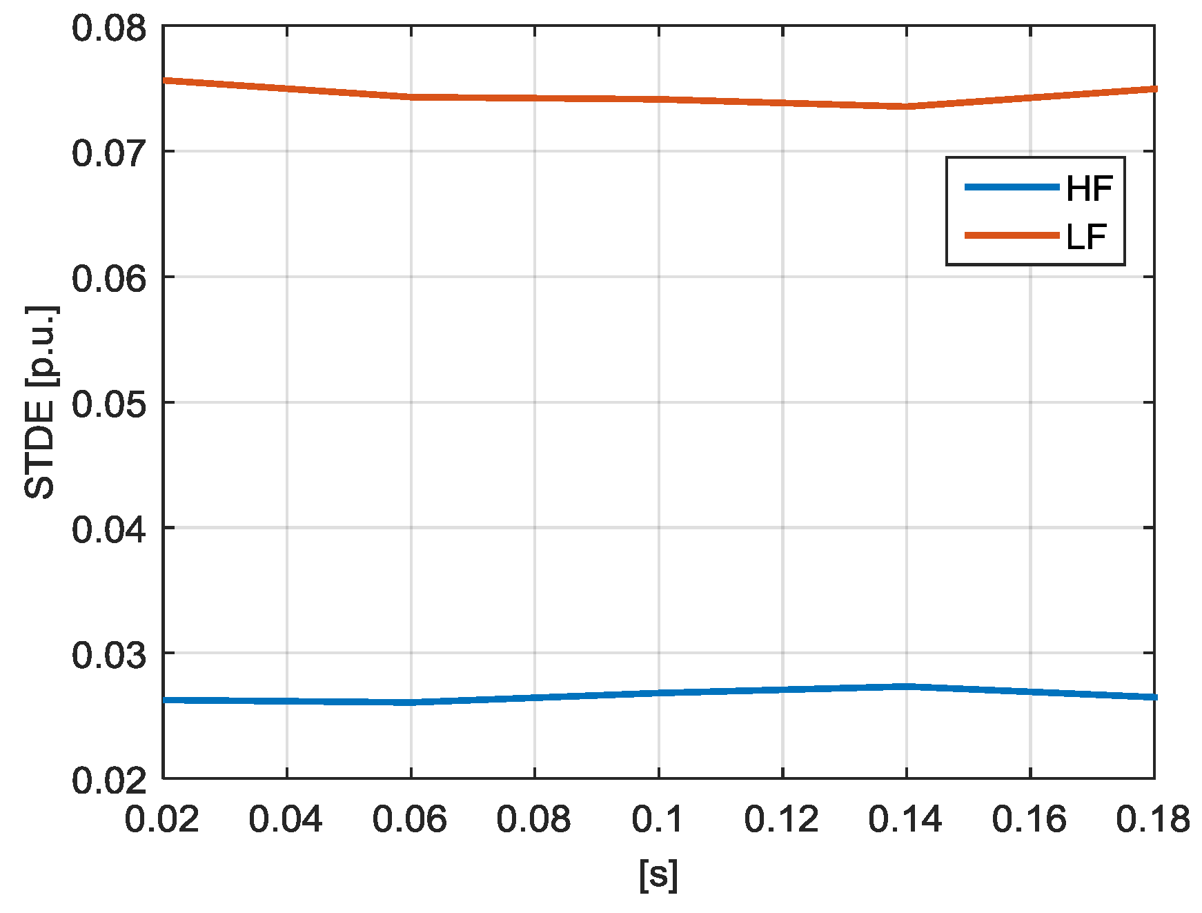
- the short time disturbance energy index for both the low- and high-frequency ( and , respectively);
- -
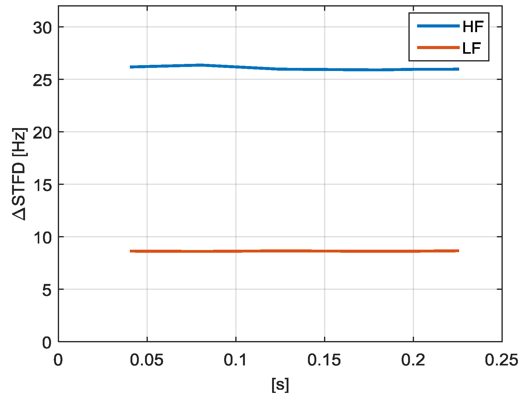
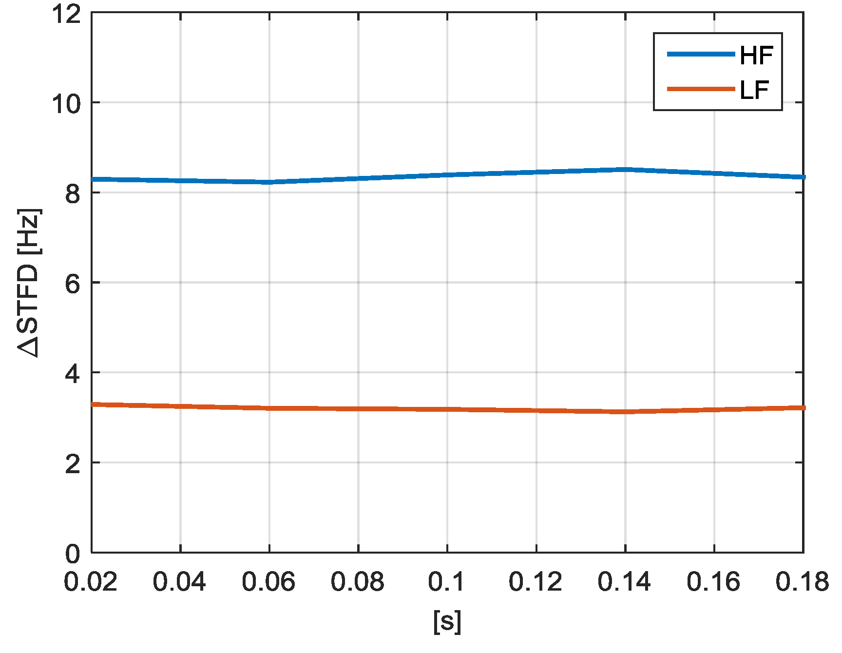
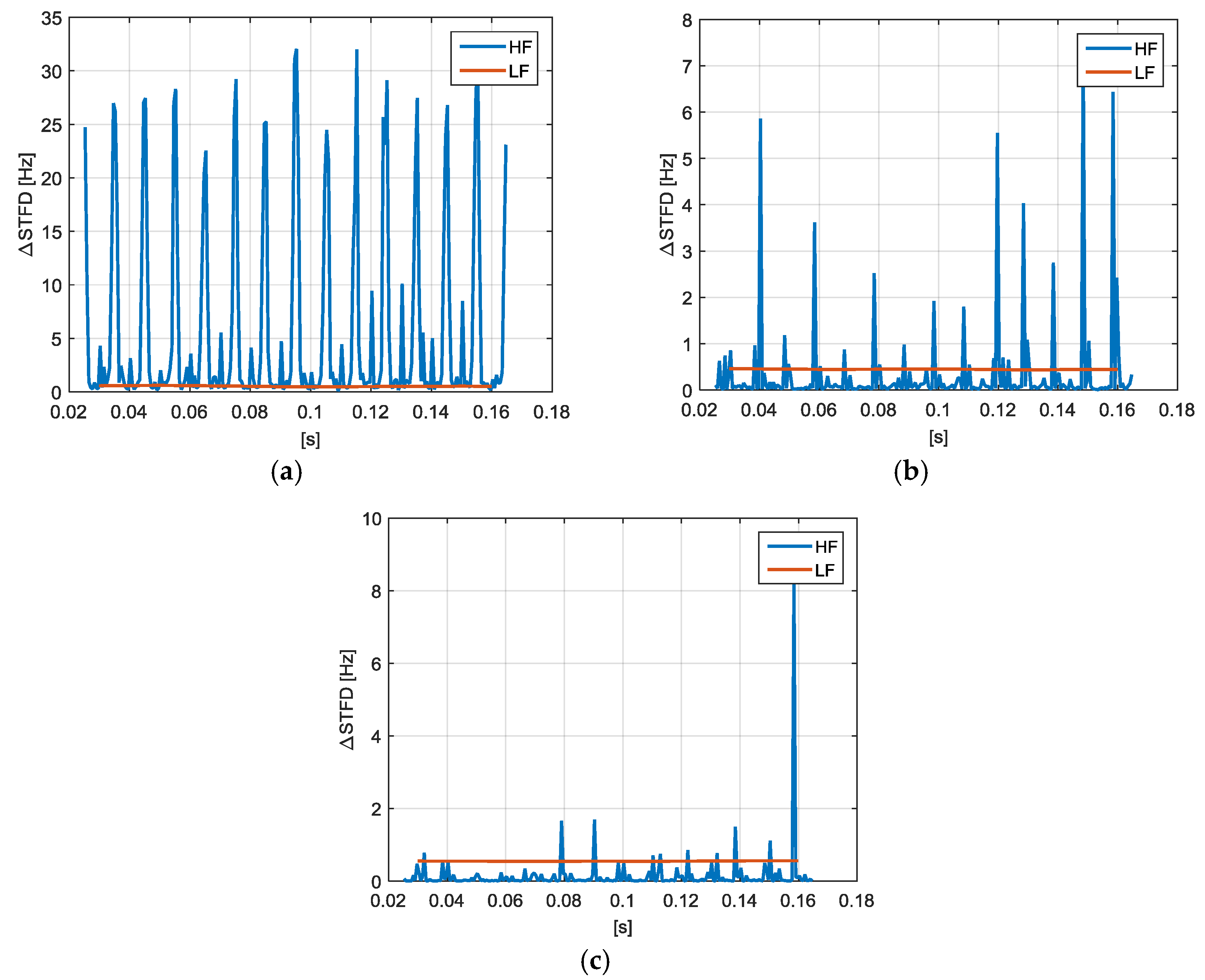
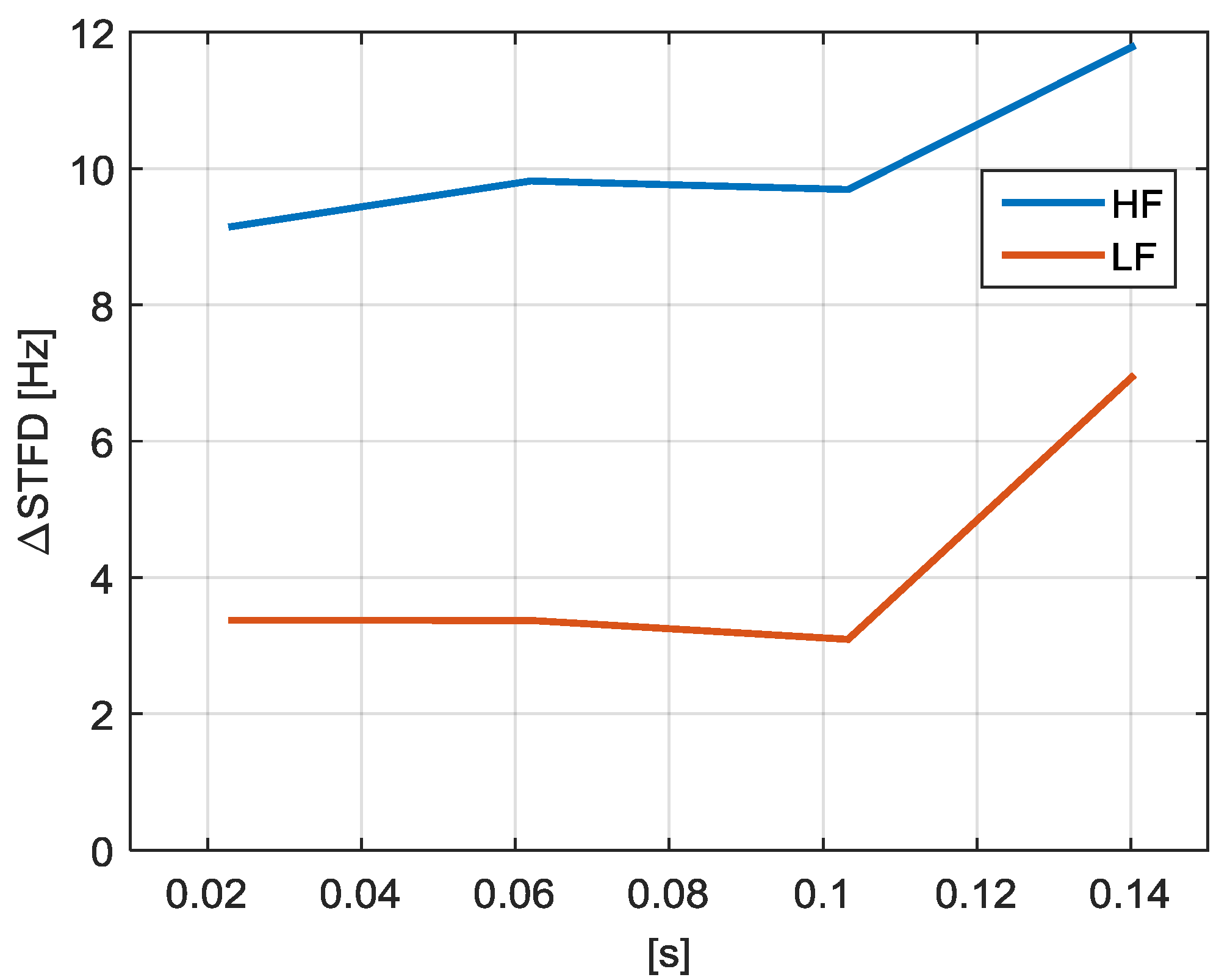
- the short time frequency deviation difference index for both the low- and high-frequency (, , respectively);
- -
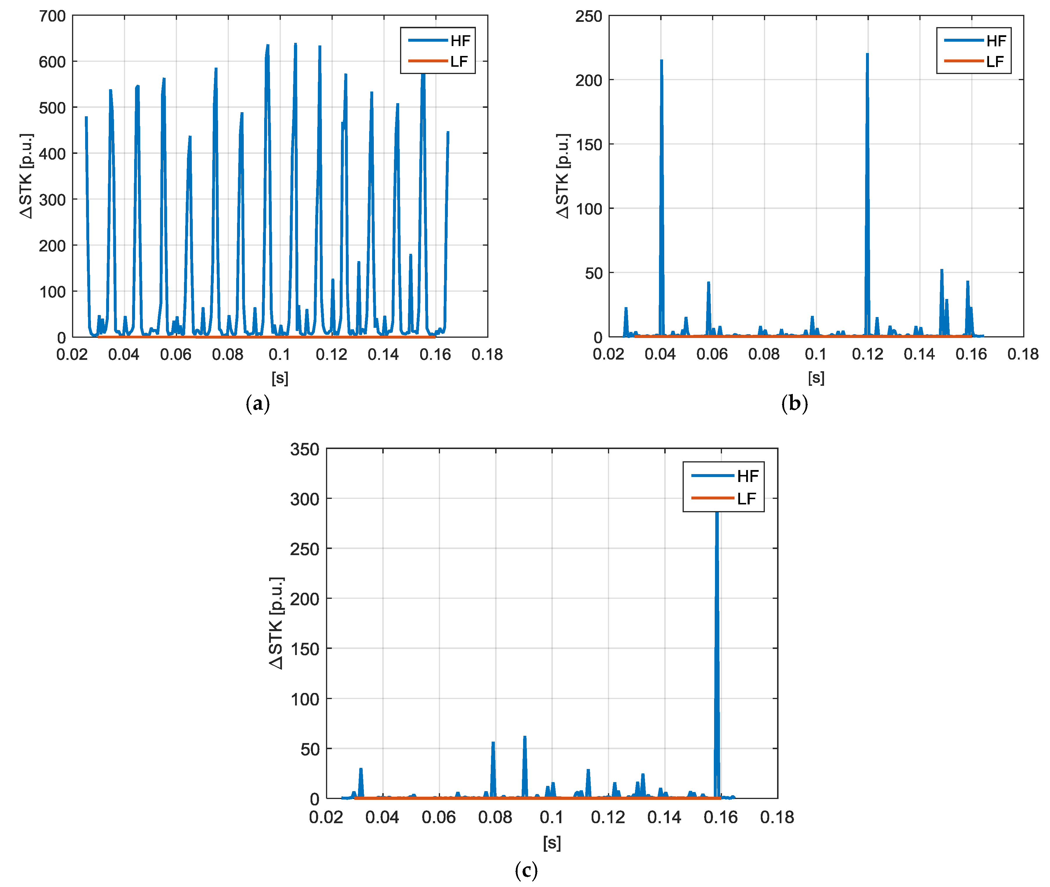
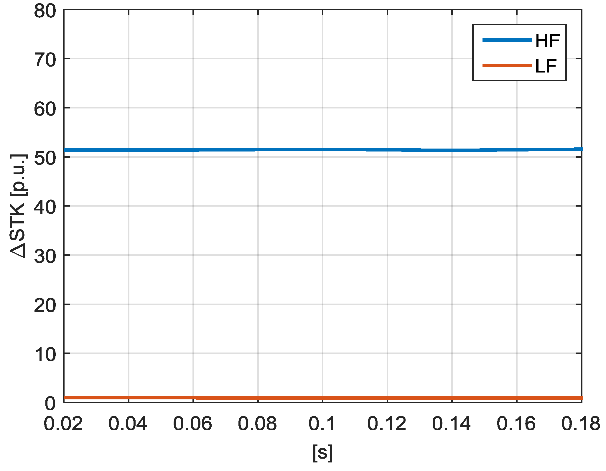
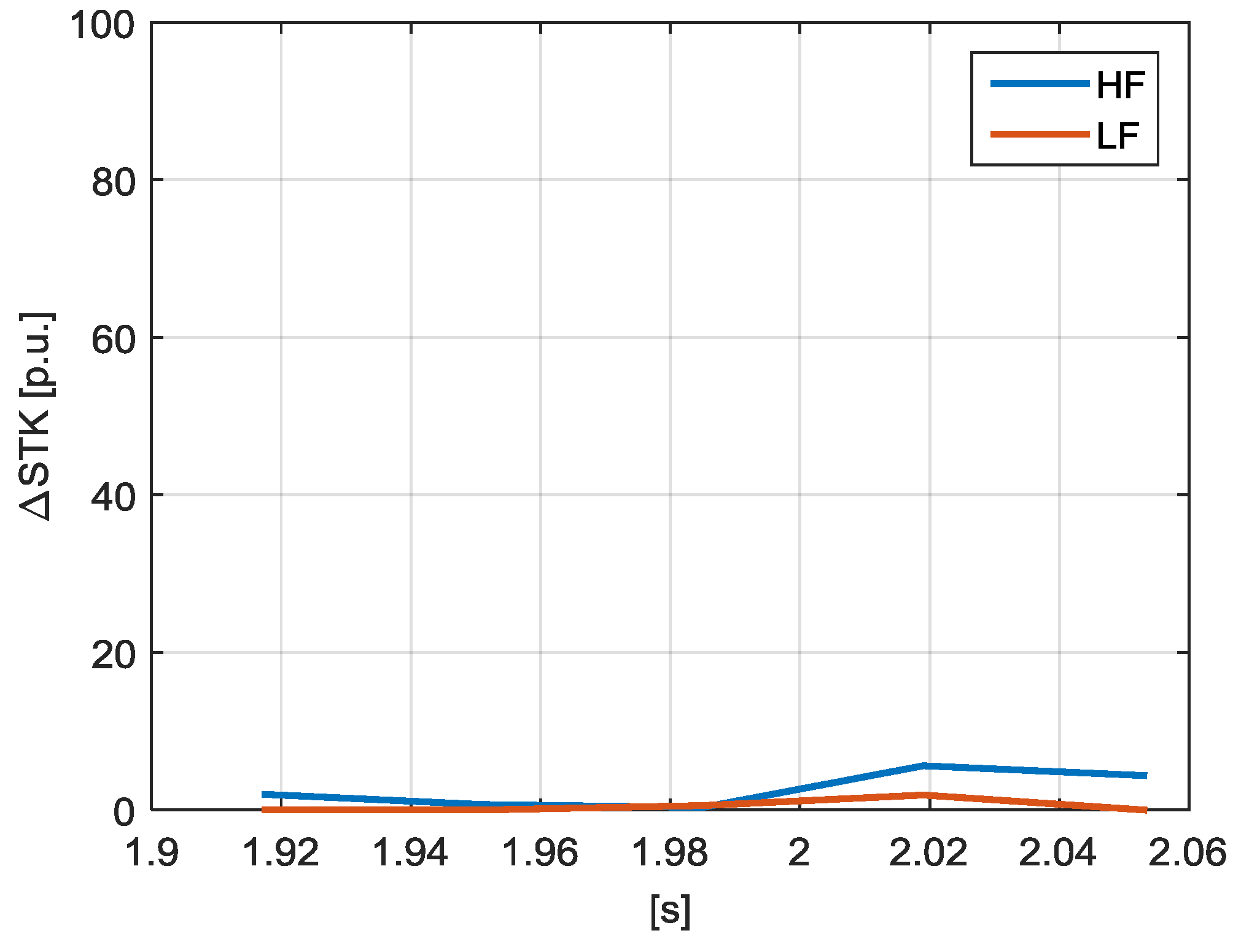
- the short time k-factor difference index for both the low- and high-frequency ( and , respectively).
- the above advantages from (i) to (v) are extended to wide-spectrum waveforms including high frequency distortions;
- low-frequency and high-frequency disturbances can be evaluated by using PQ indices which can be calculated using different sliding time window lengths leading to more adequate quantification of disturbances;
- SWWMEM may be applied to the whole wide-spectrum waveform, from which all the quantities needed for the calculation of the new PQ indices are provided;
- the analyzed waveform can be classified, since an assessment of the main disturbance allocation between low-frequency and high-frequency distortions is provided.
2. High-Frequency Distortions in Power Systems
3. Proposed PQ Indices
- -
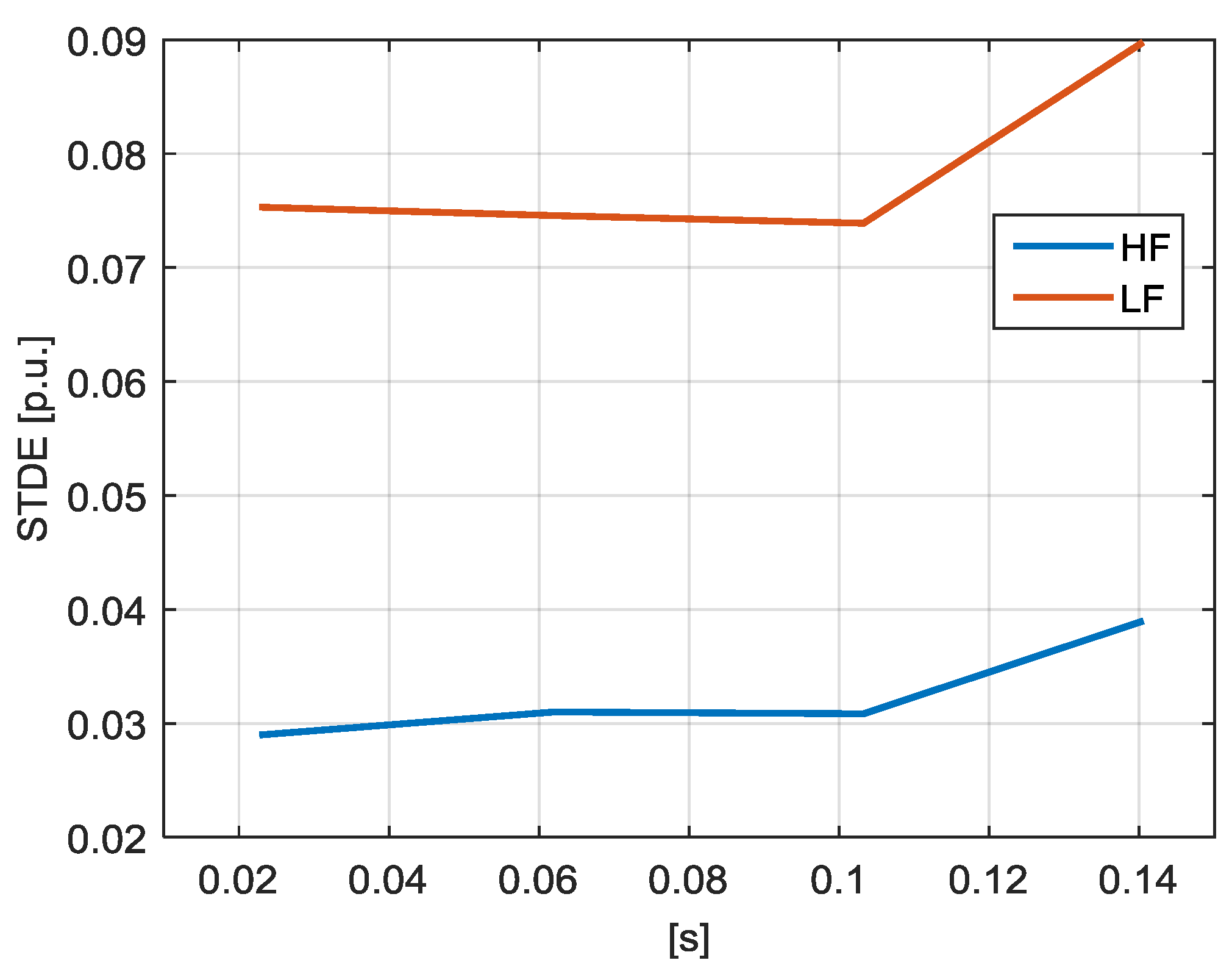
- the STDE is a short-time version of the THD, but, differently from the THD, it performs the distortion quantification by taking into account the energy related not only to the harmonics, but to the whole spectral content included in the waveform;
- -
- the STFD provides a measure of the severity of the highly varying disturbances, weighting each frequency included in the waveform spectrum with the energy content corresponding to that spectral component, in order to estimate the deviation of the instantaneous frequency of the waveform from the power system frequency;
- -
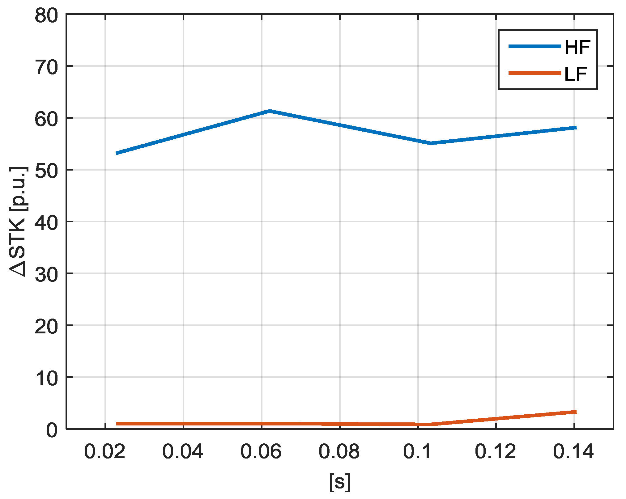
- the STK is the generalization of the k-factor to the whole spectral content included in a waveform, and it is commonly utilized for transformer rating. It is evaluated by weighting the energy density of each spectral component by the square of the normalized frequency.
4. Numerical Applications
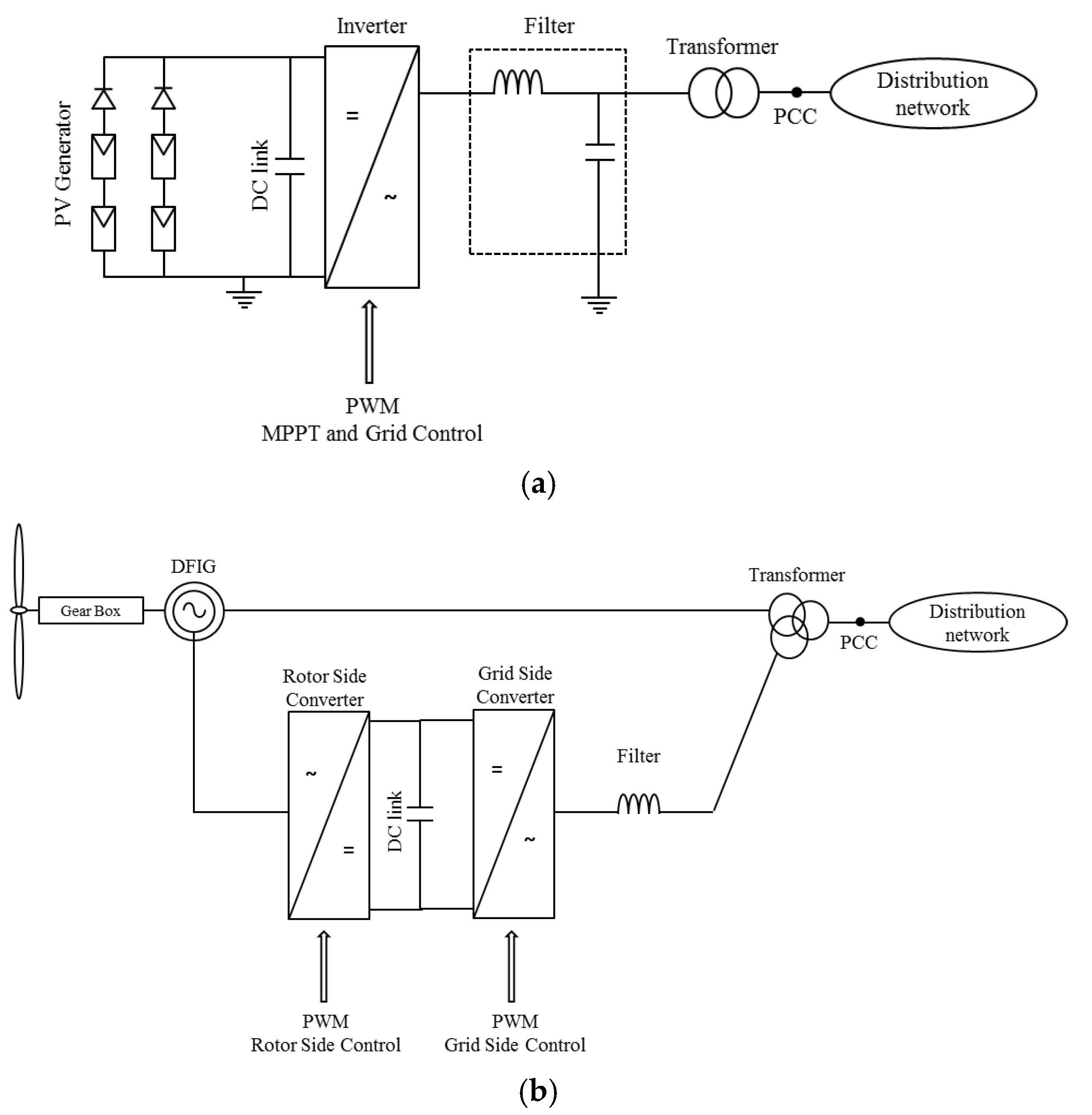
4.1. Renewable Generation
4.1.1. Case Study 1
4.1.2. Case Study 2
4.1.3. Case Study 3
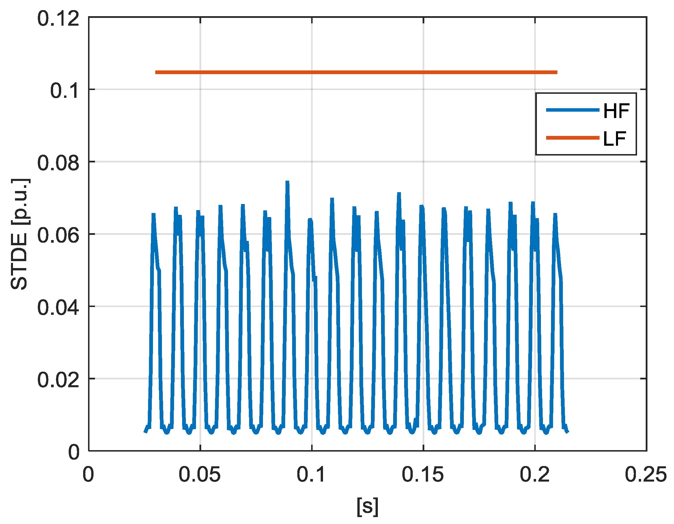
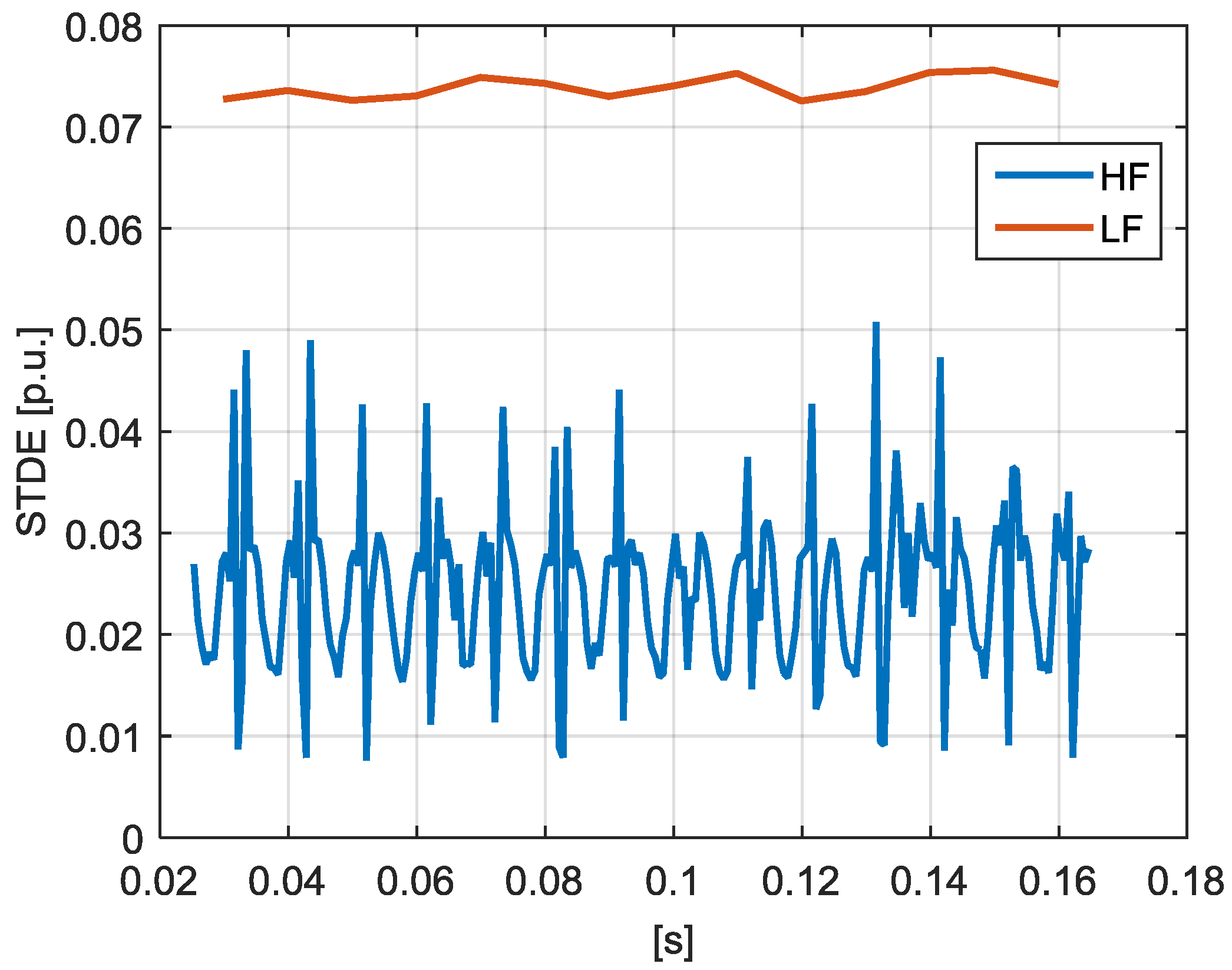
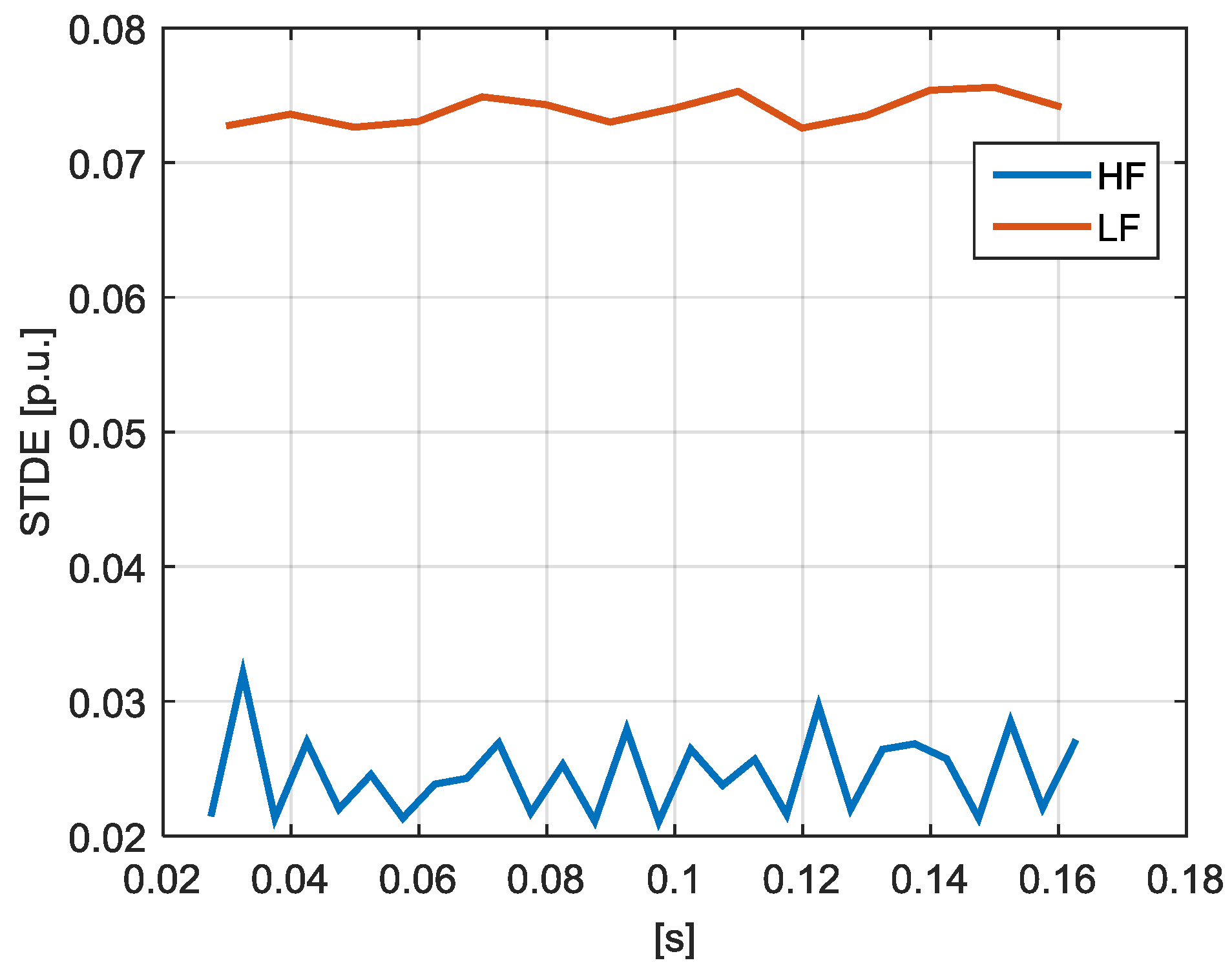
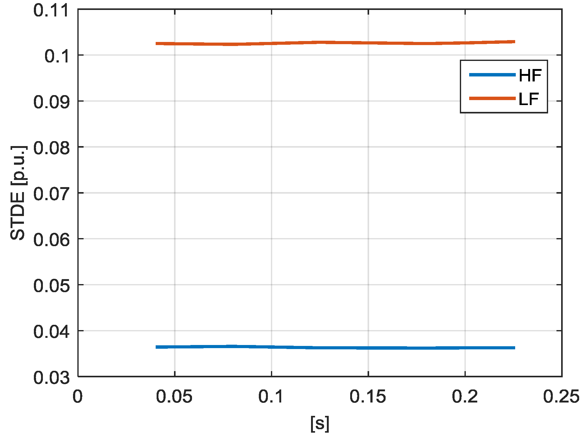
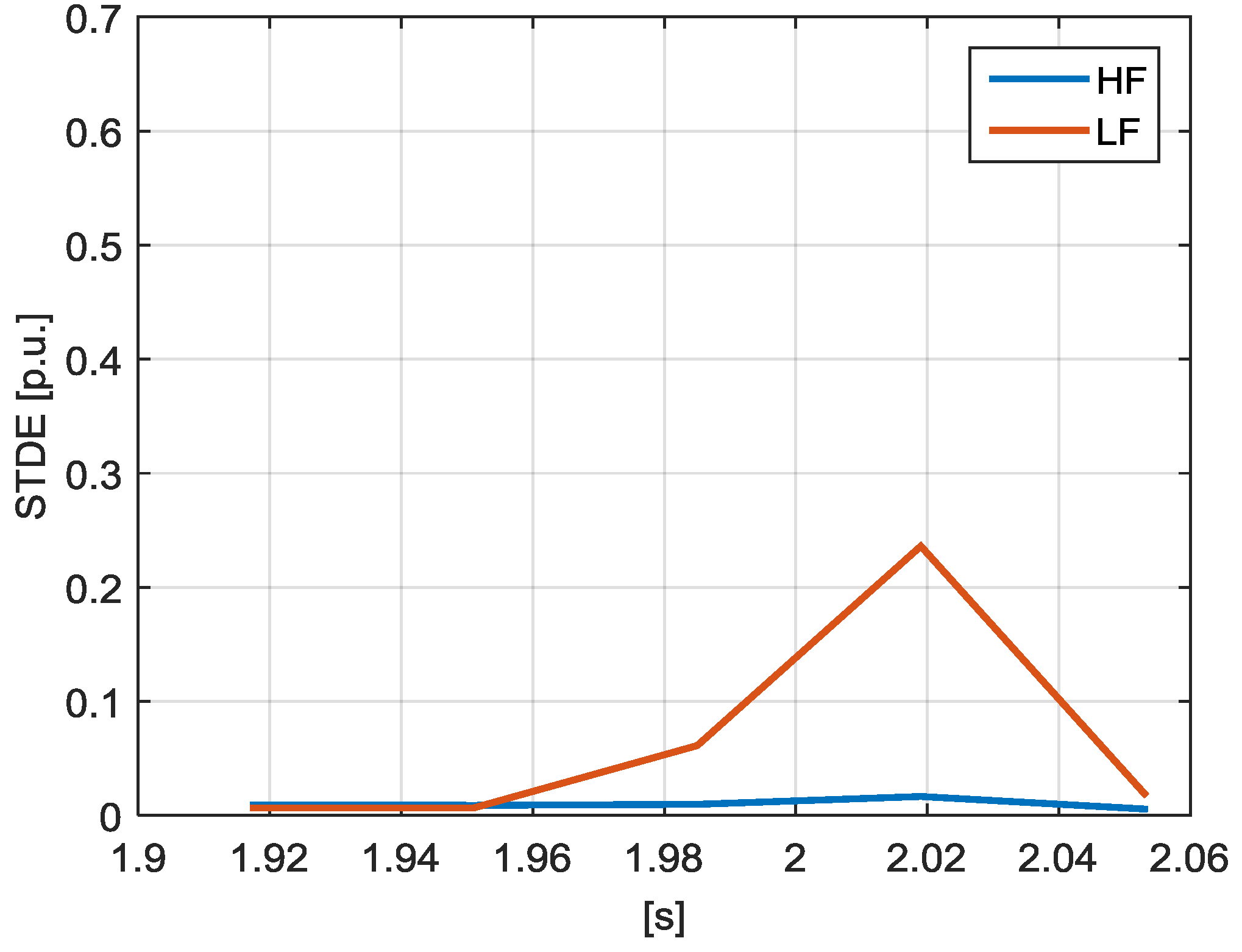
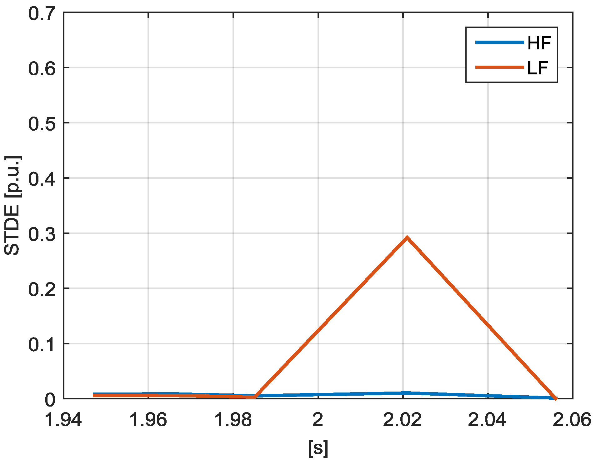
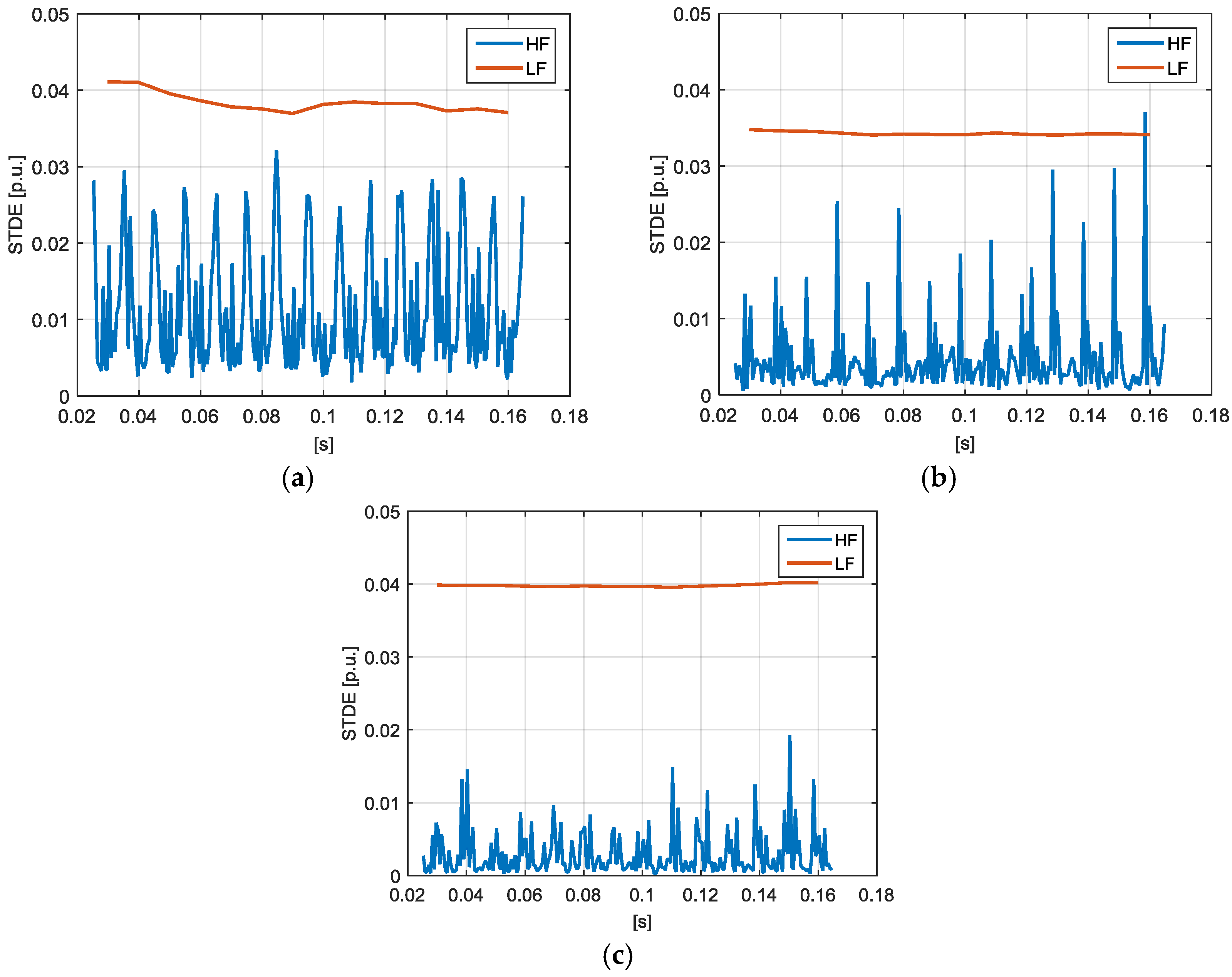
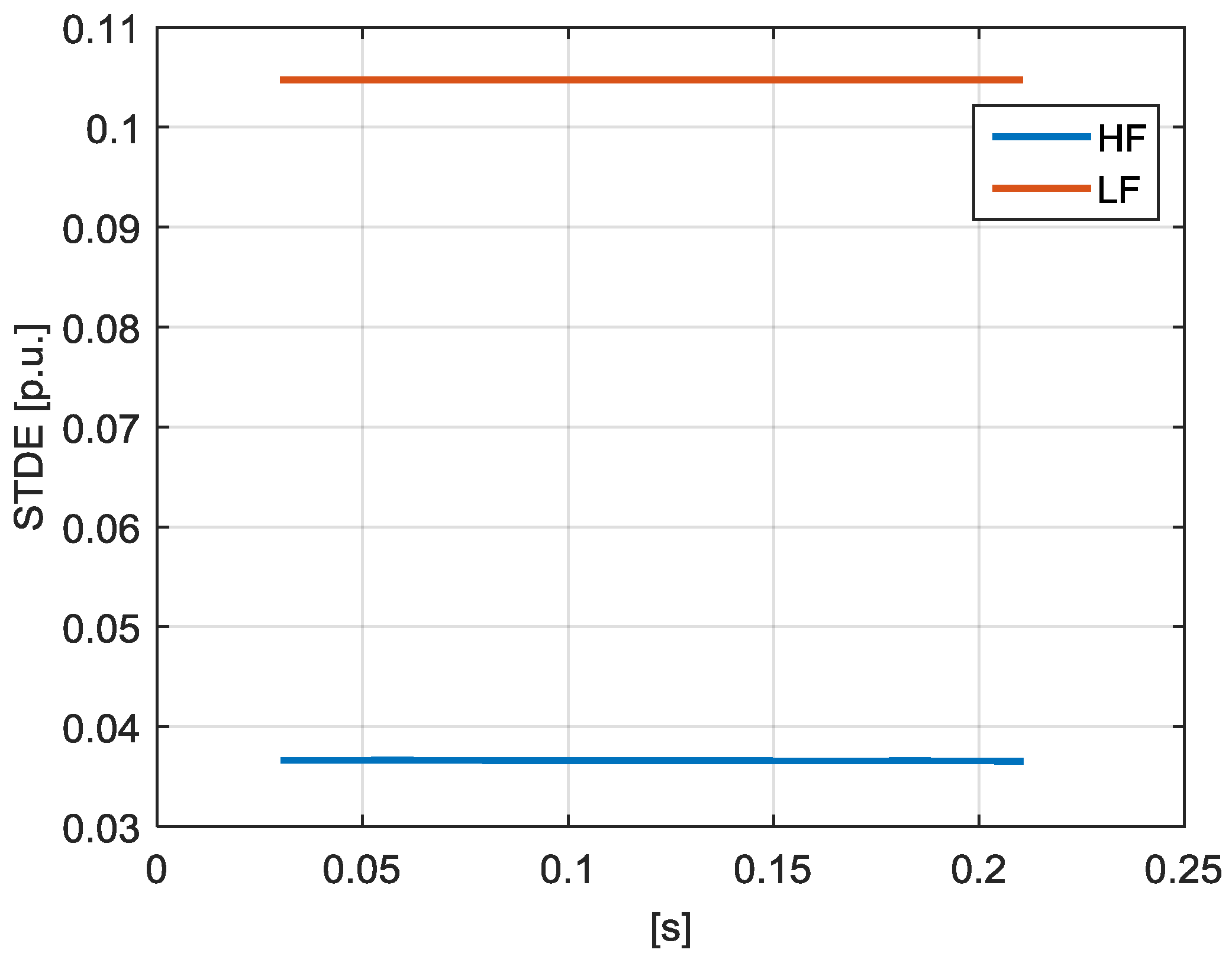
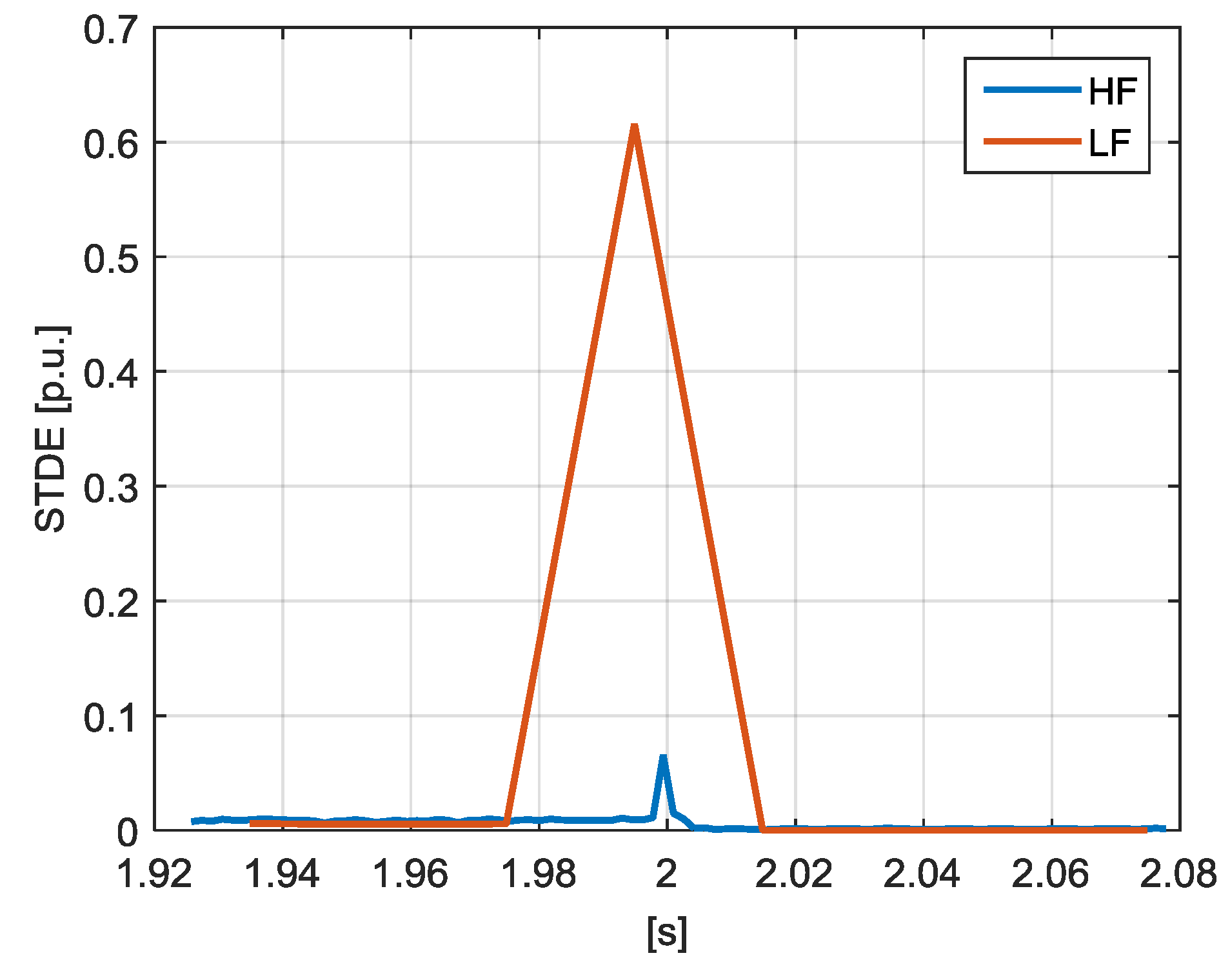
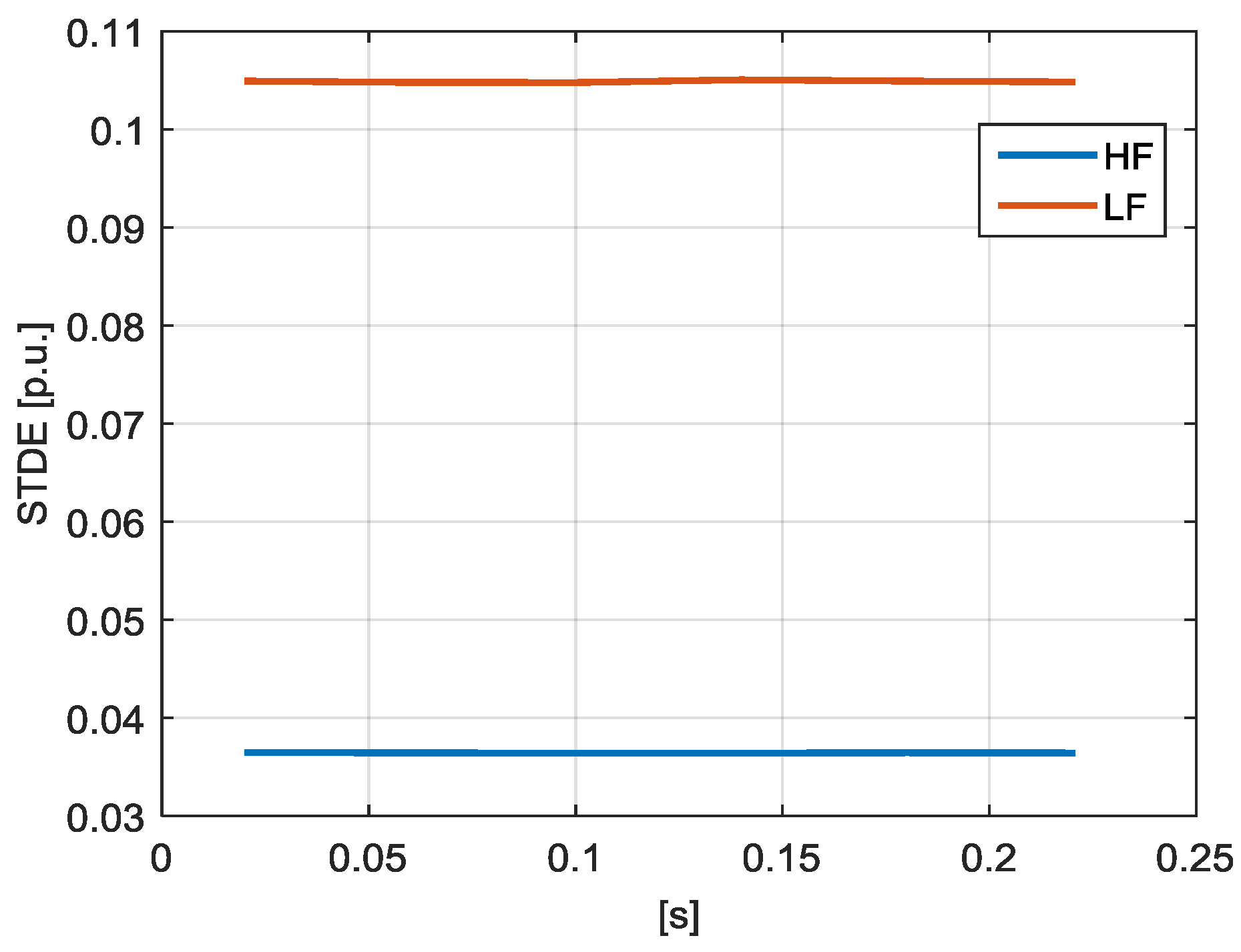
- Figure 19 shows for (red line) a peak value equal to 0.62 p.u. corresponding to the transient, while for (blue line) the peak value of the transient is equal to 0.065 p.u.;
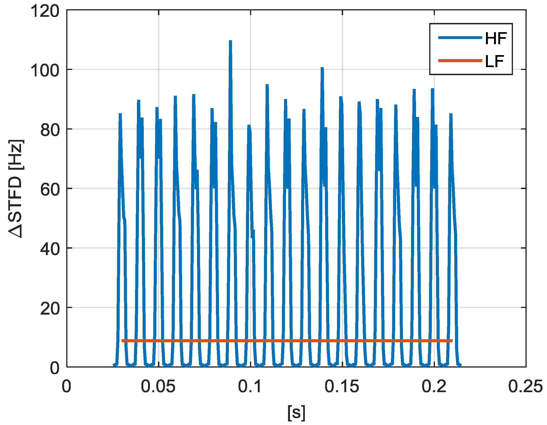
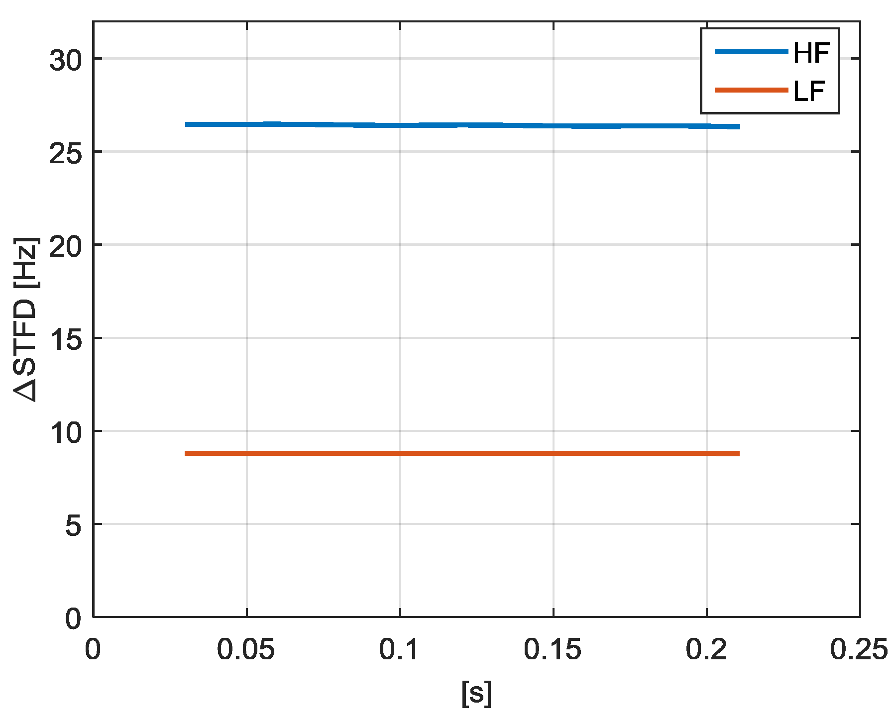
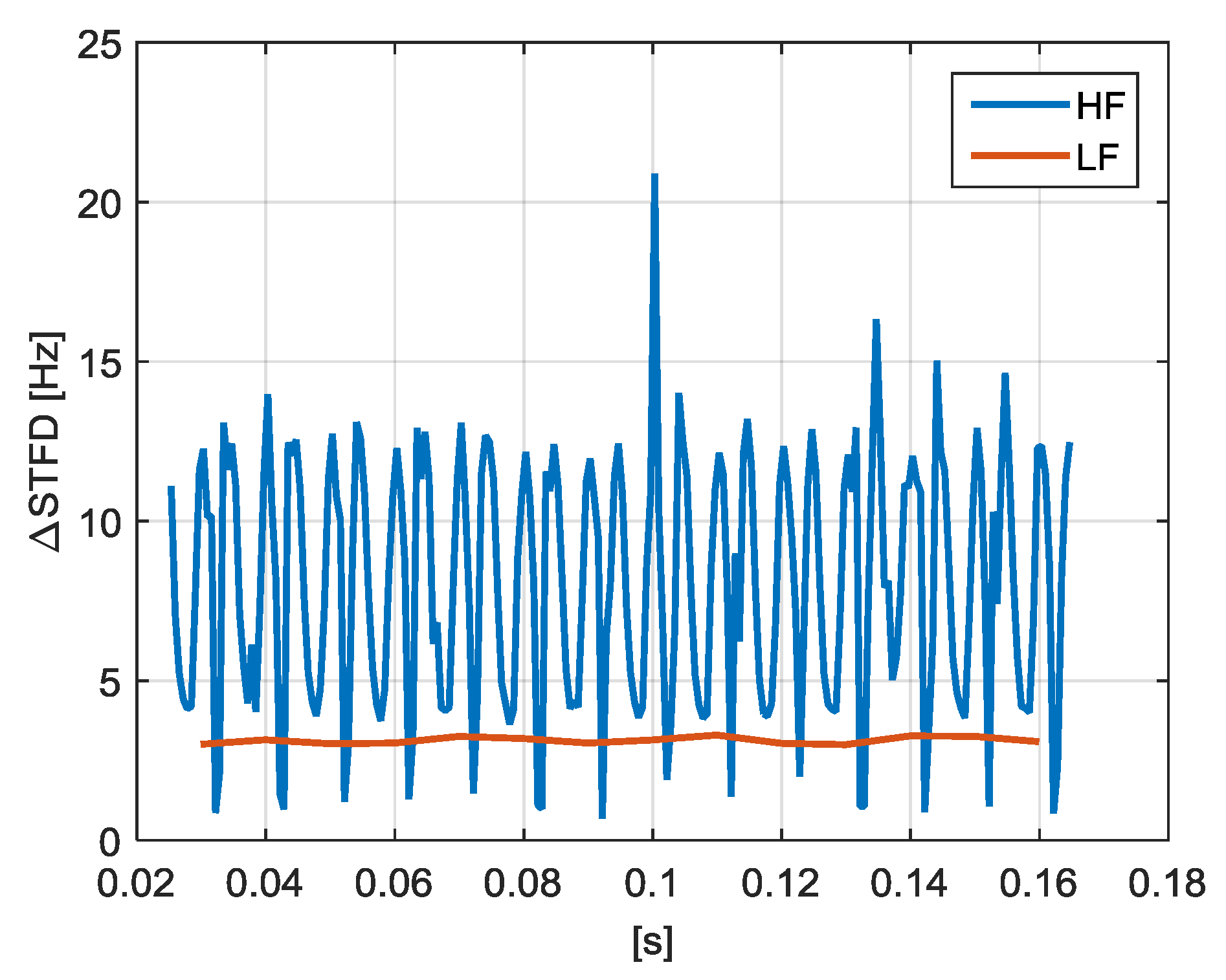
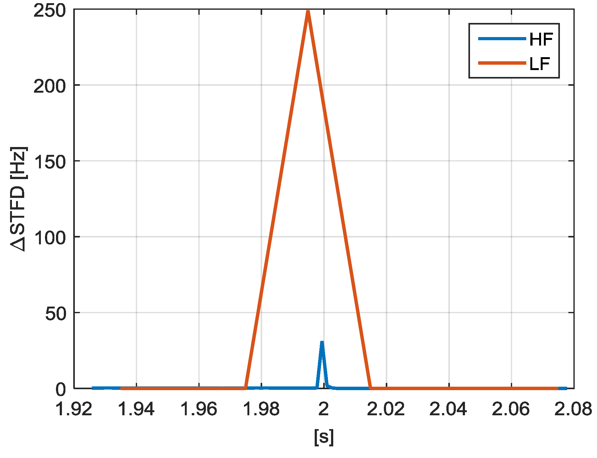
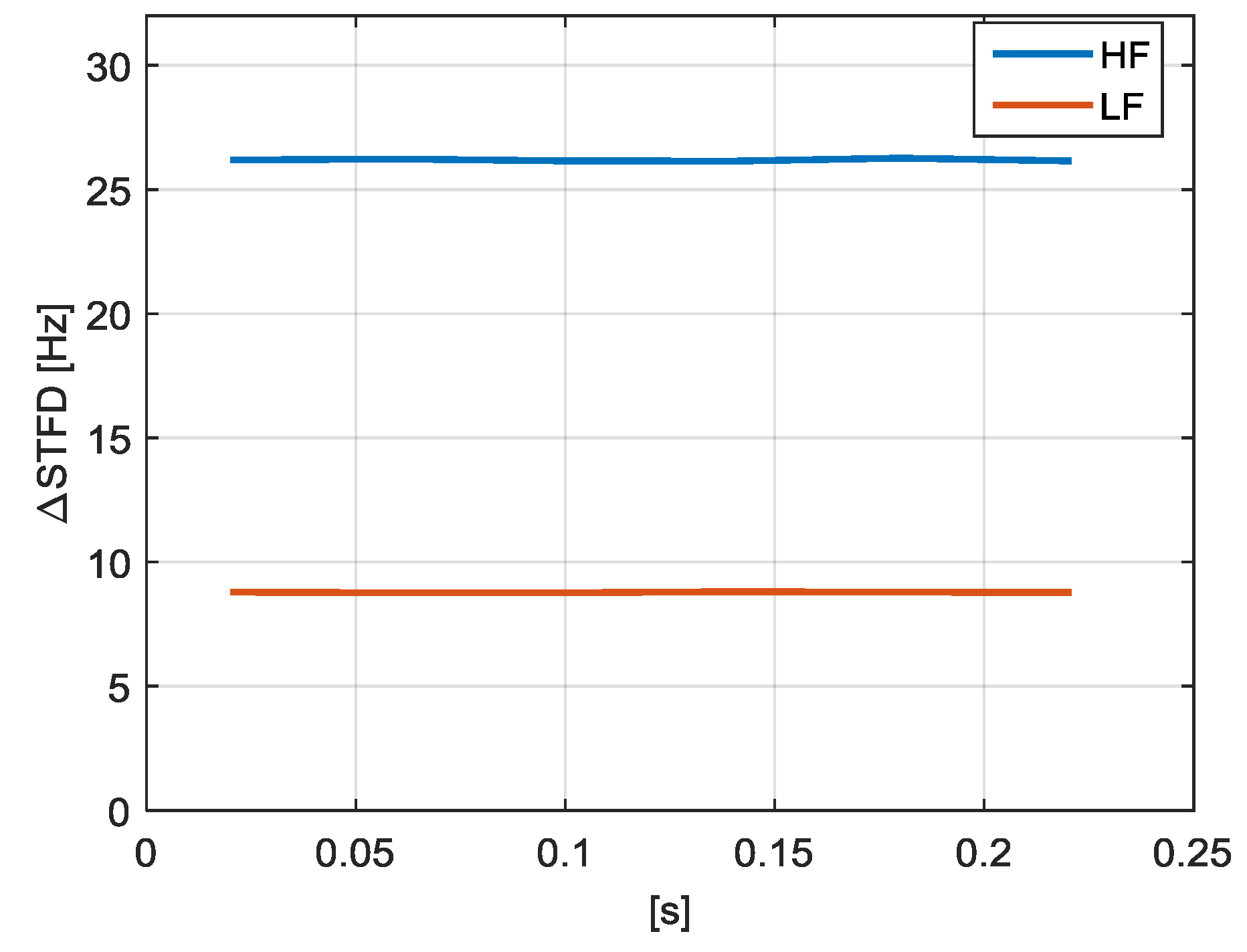
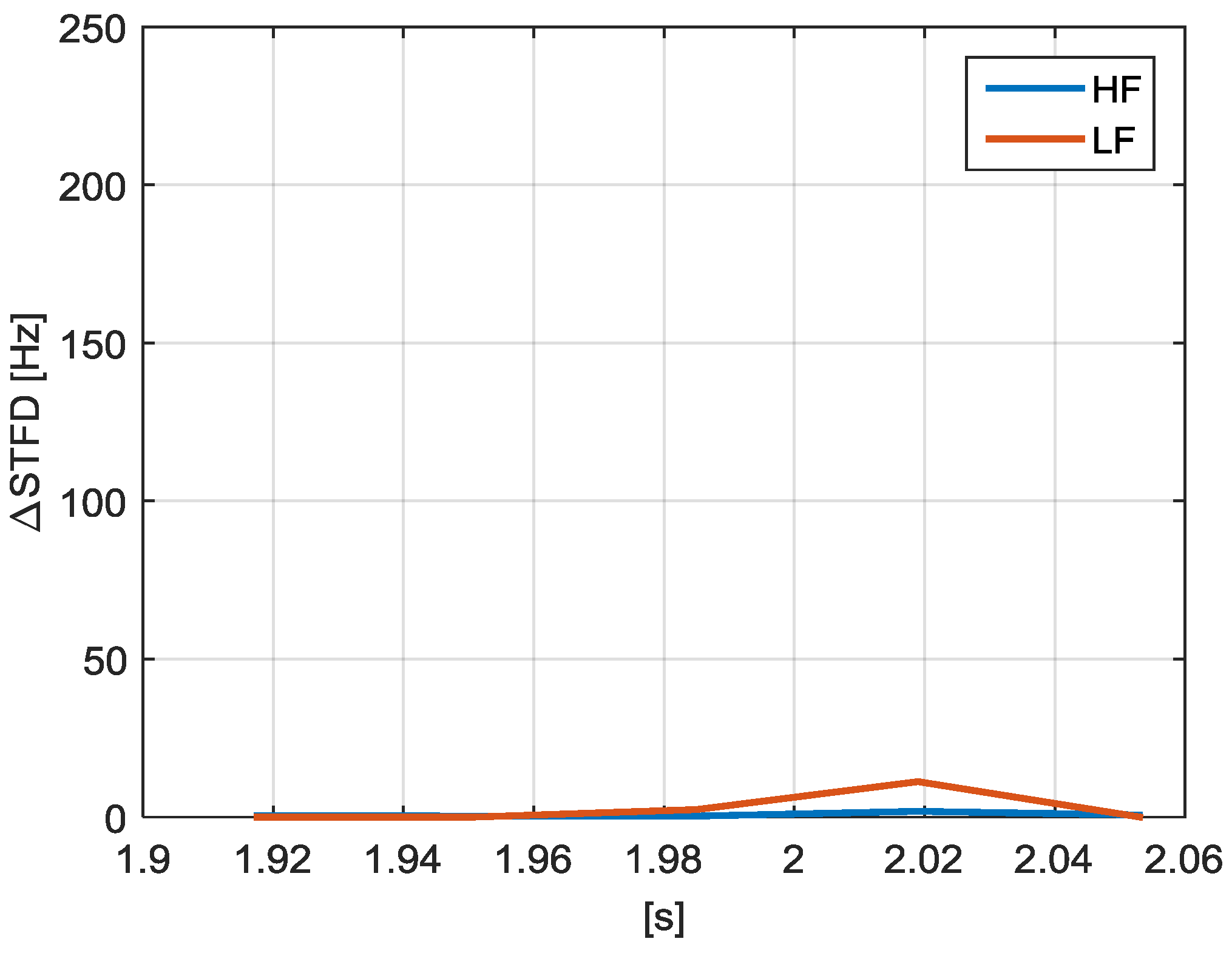
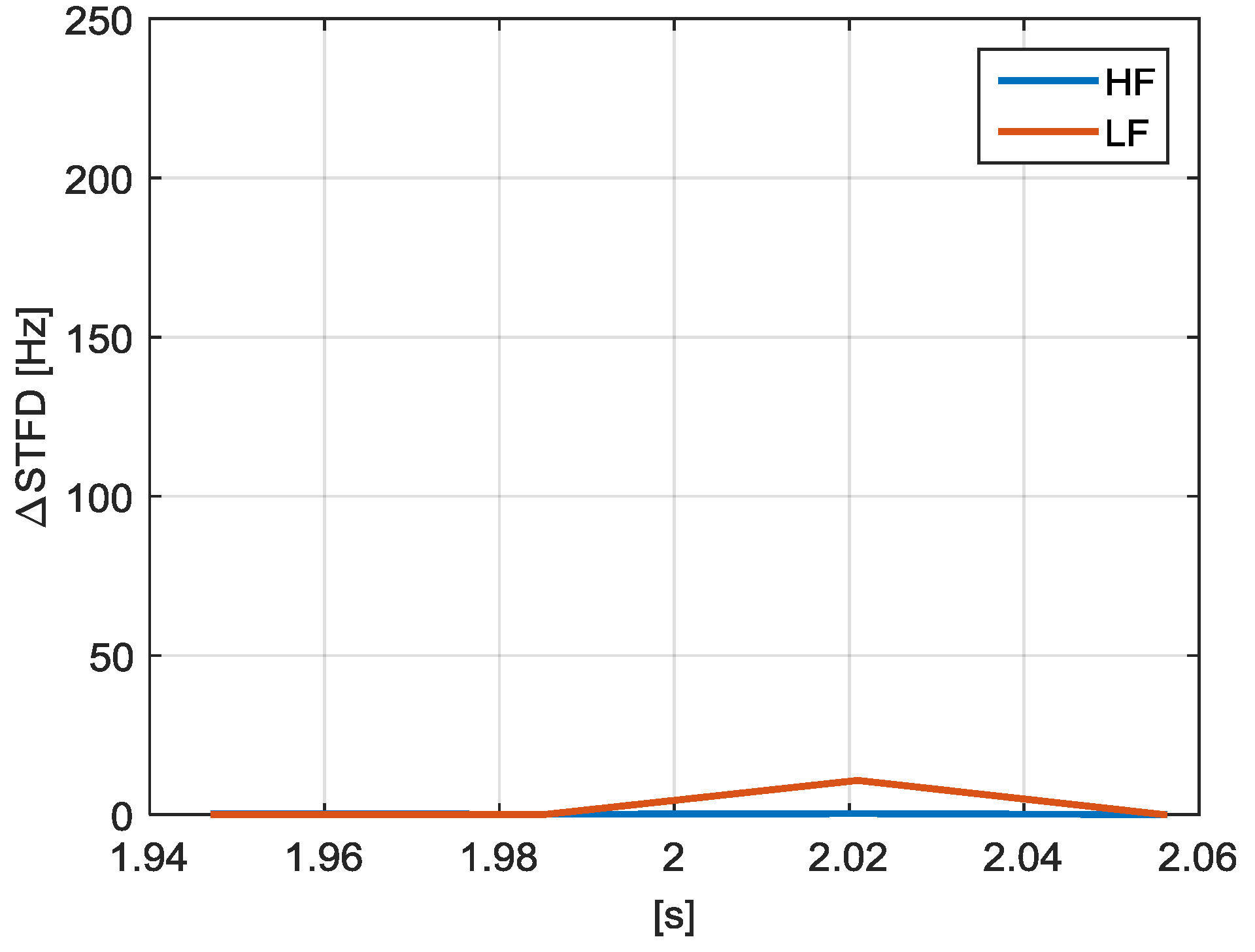
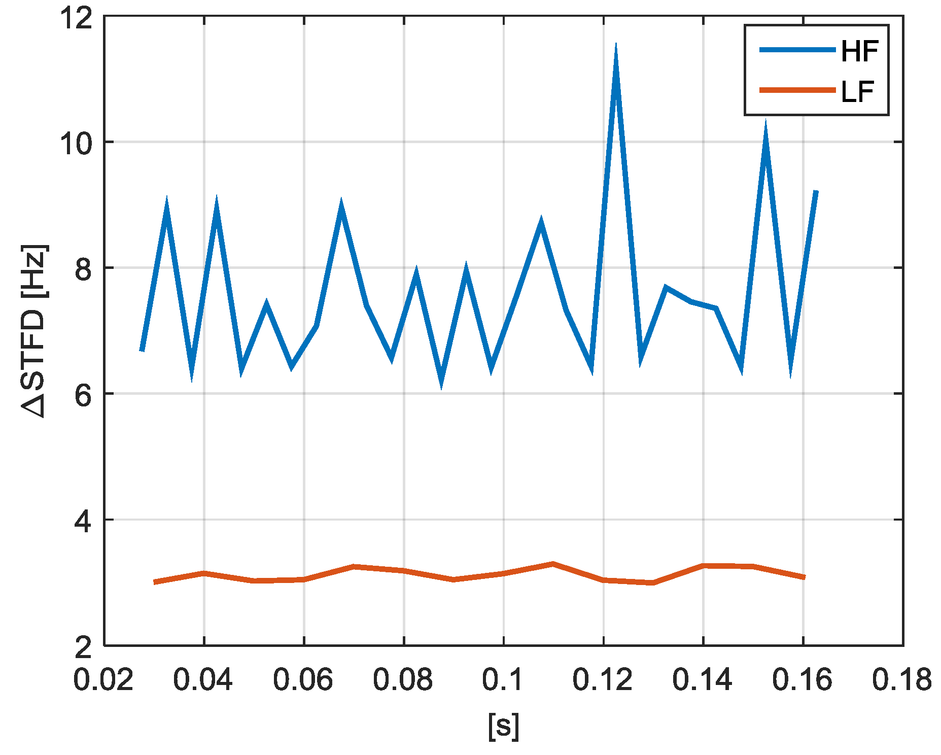
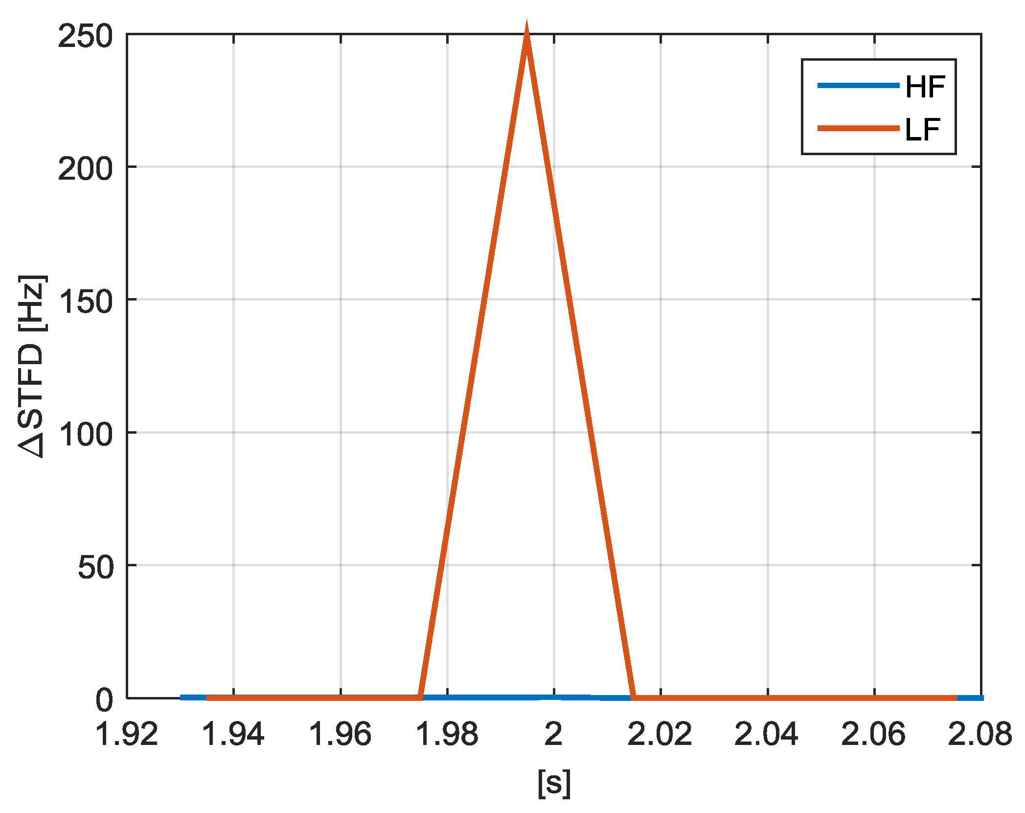
- Figure 20 shows for (red line) a peak value equal to 249.10 Hz corresponding to the transient, while for (blue line) the peak value of the transient is equal to 31.10 Hz;
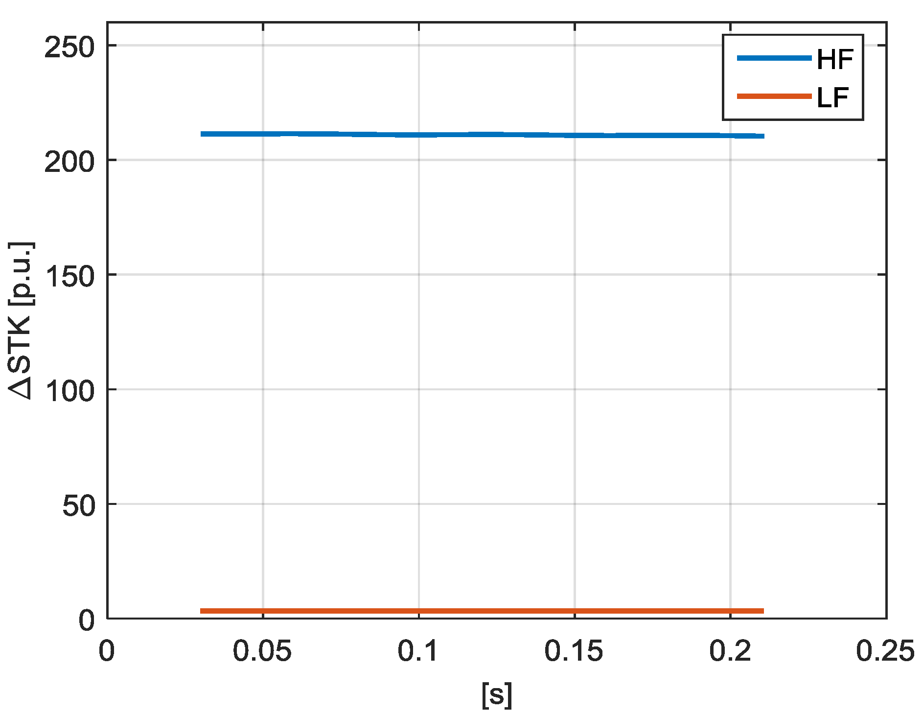
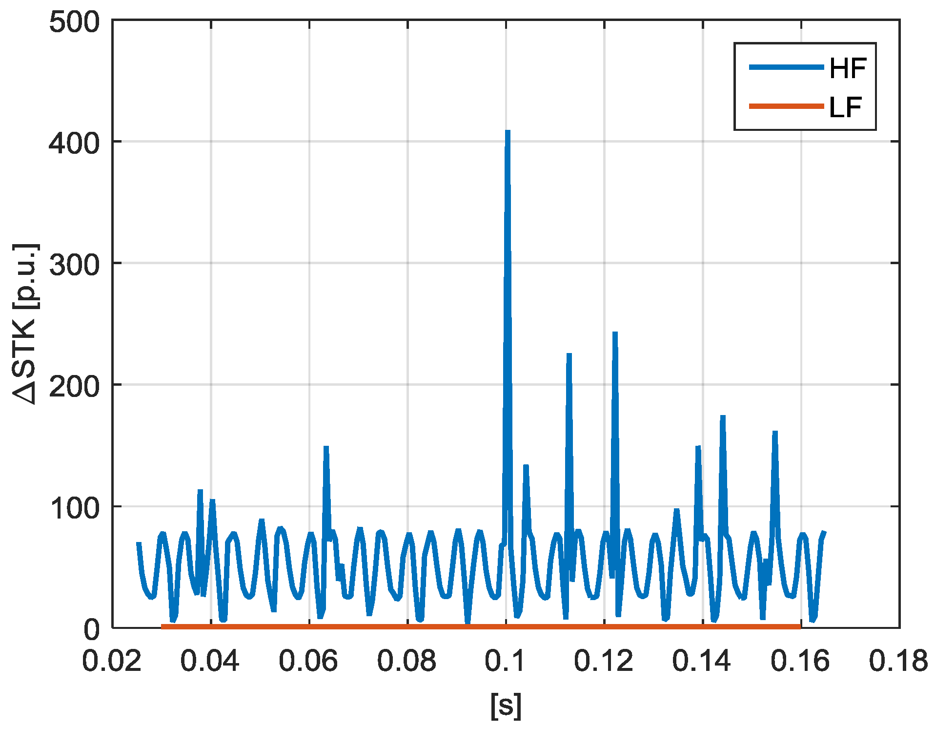
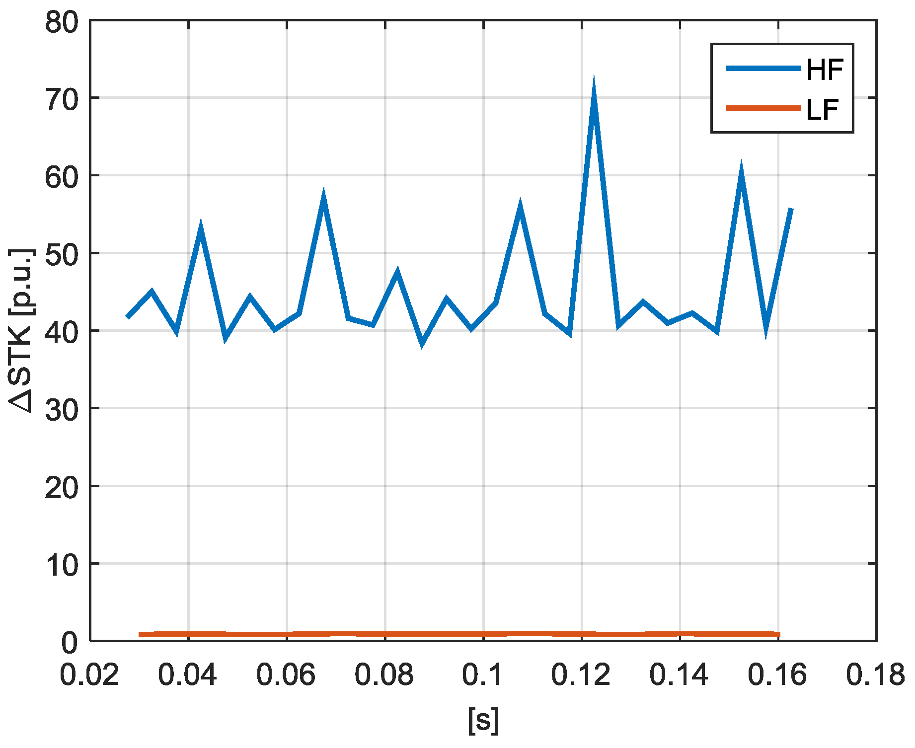
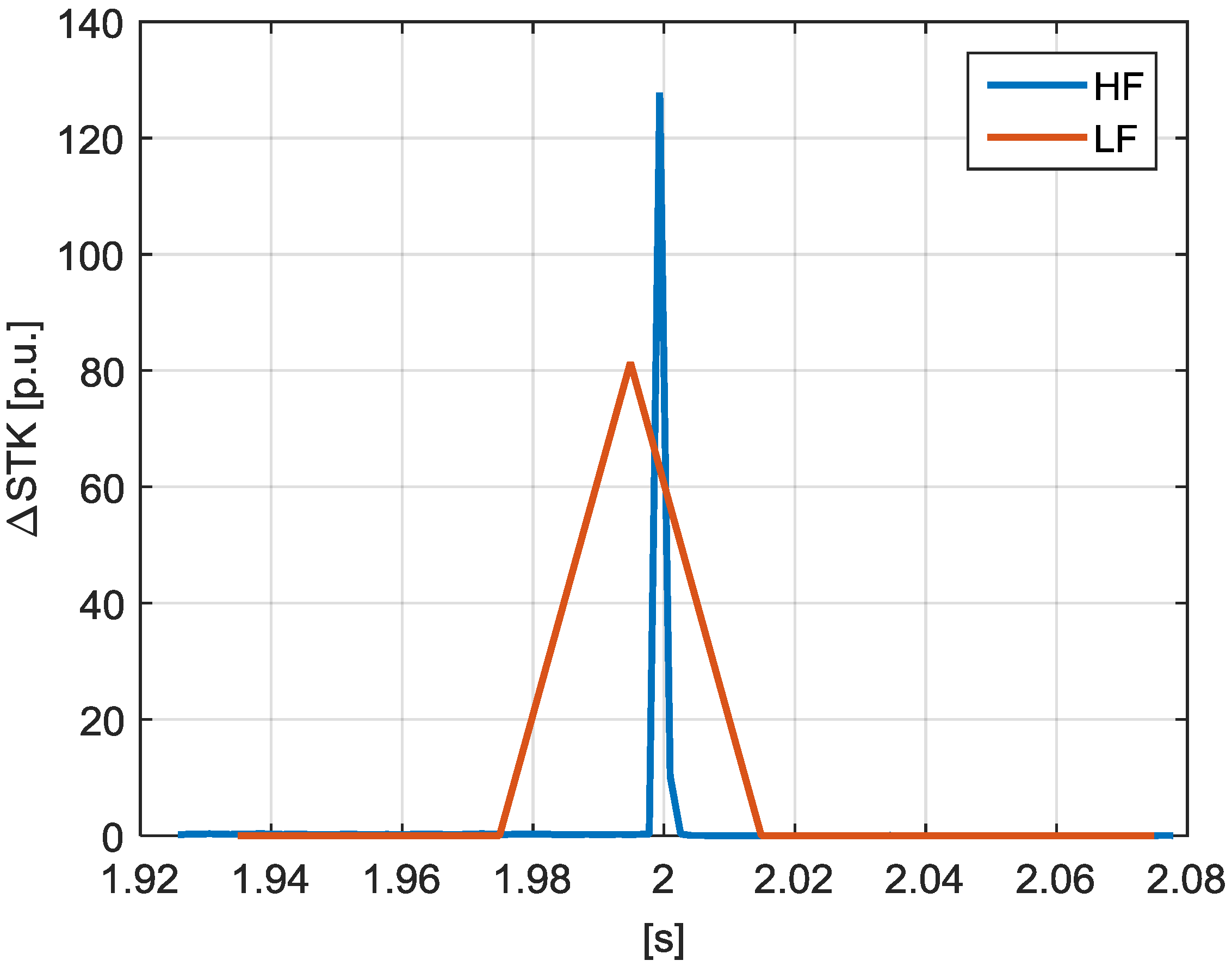
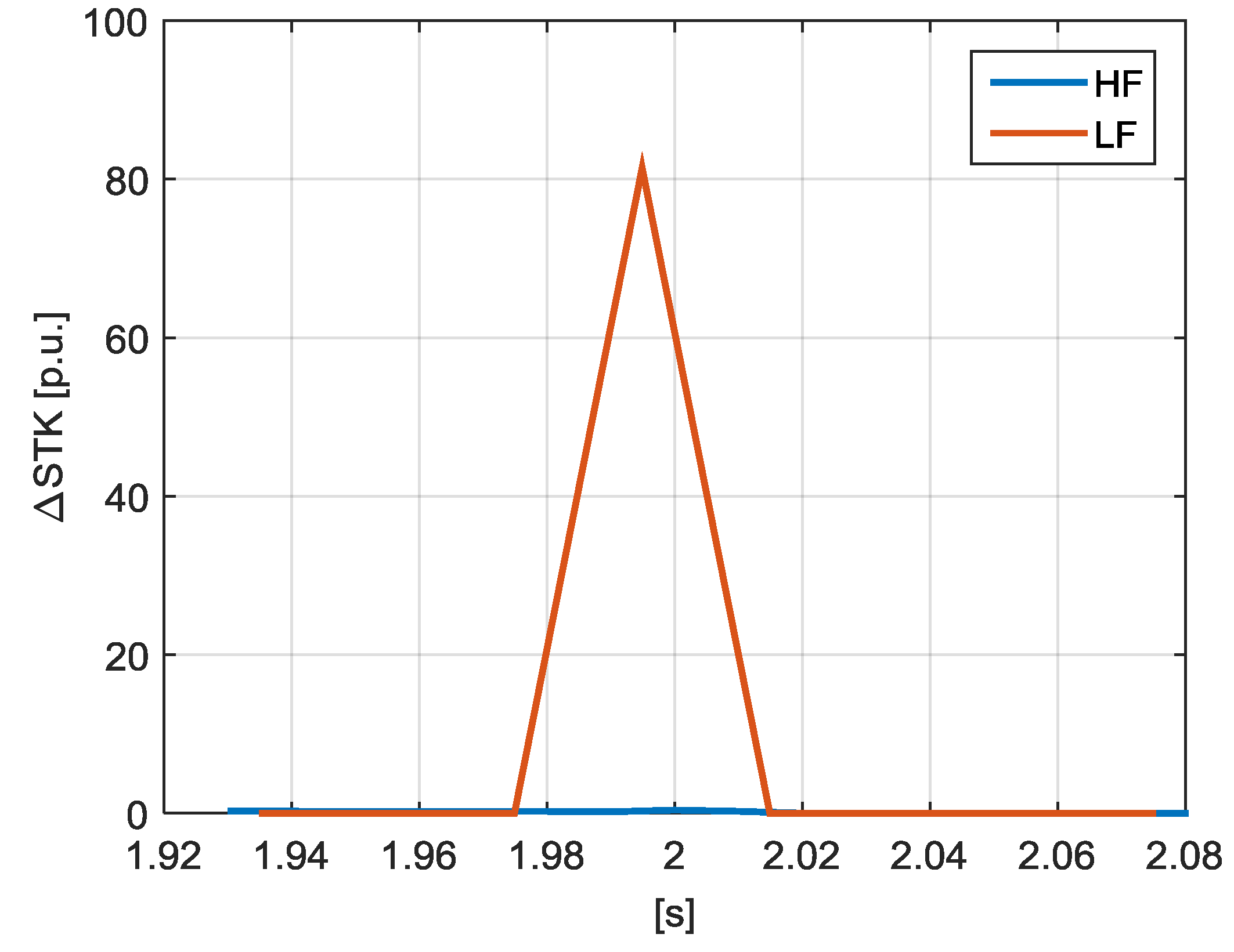
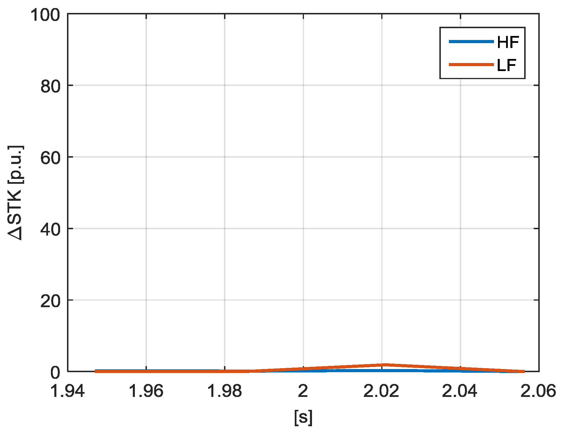
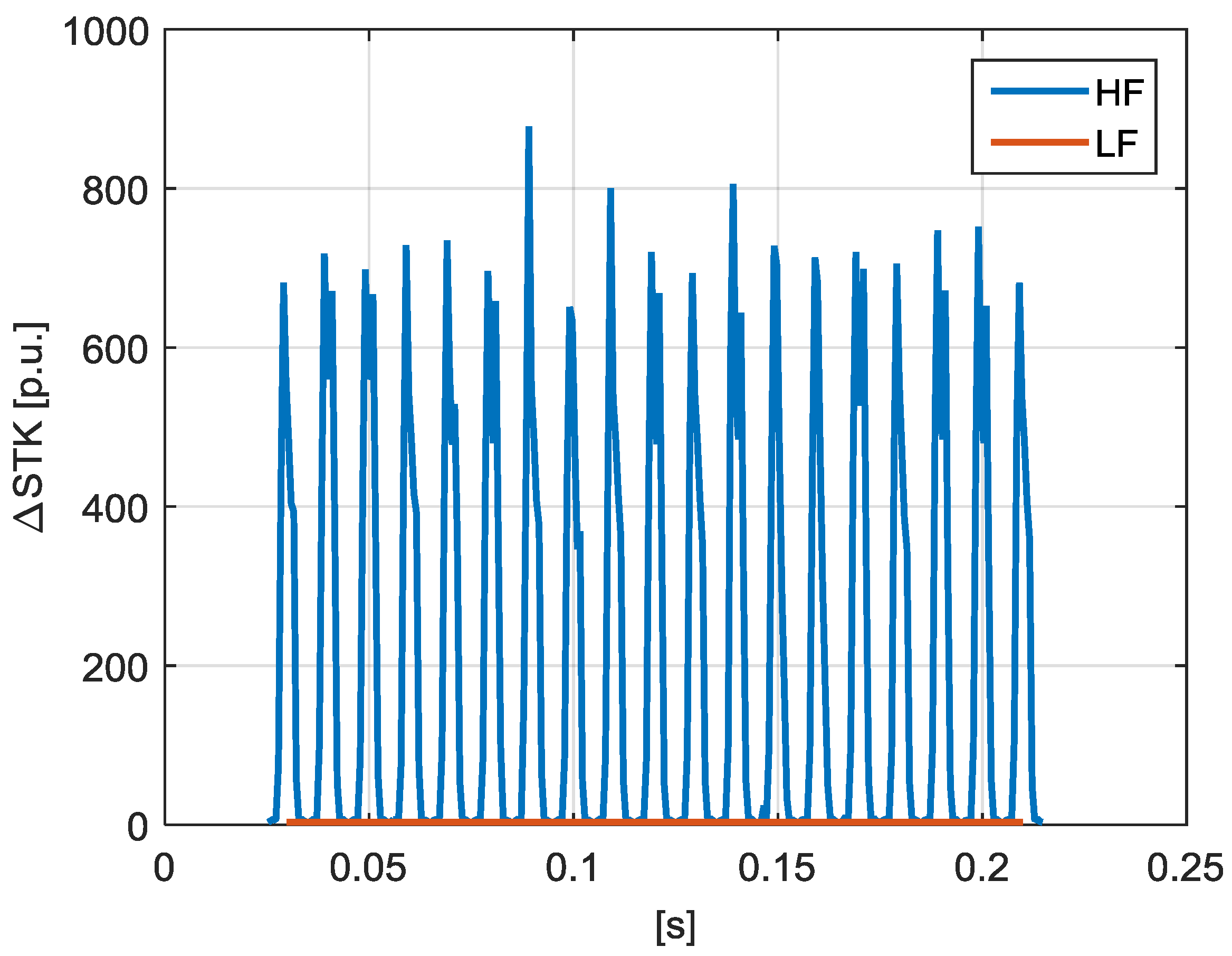
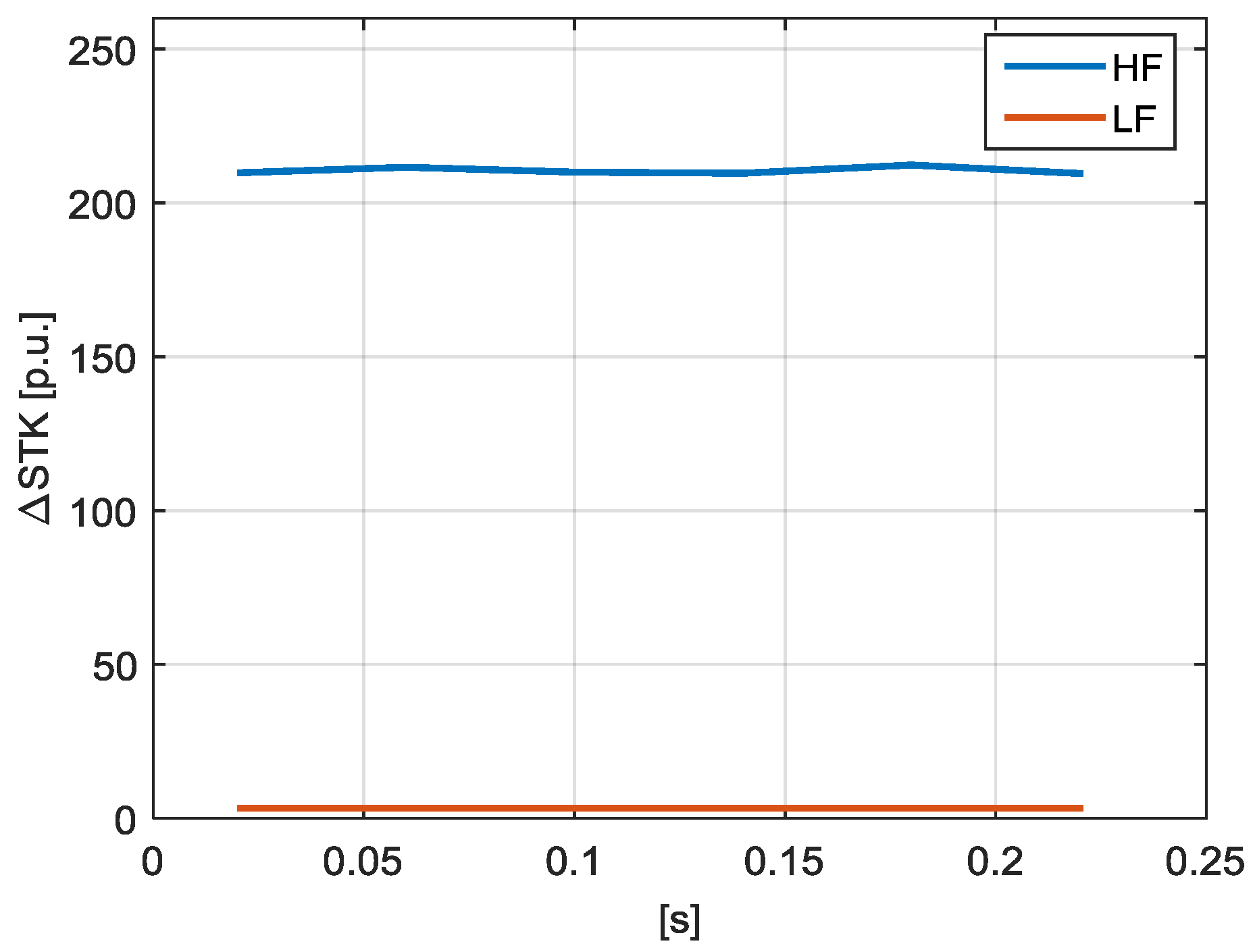
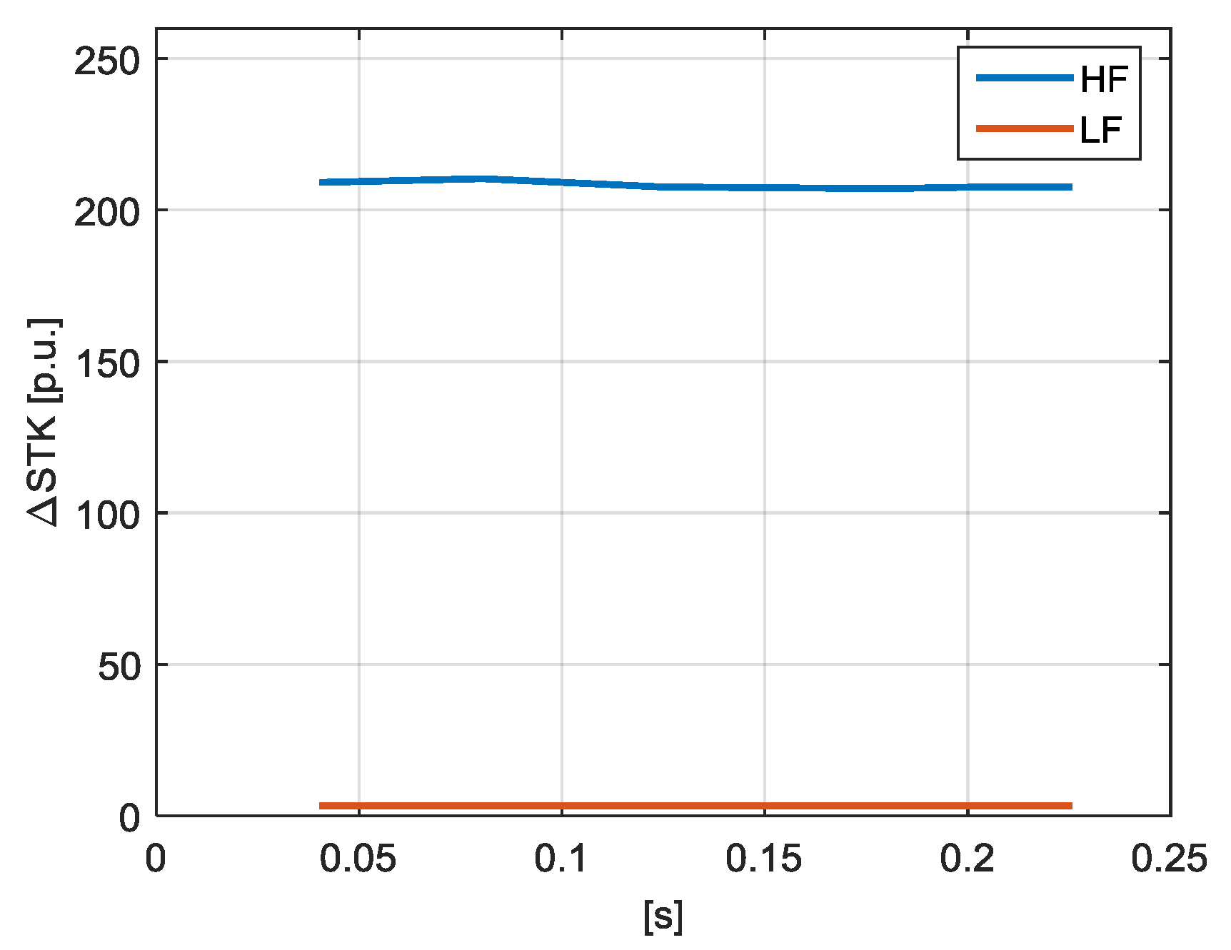
- Figure 21 shows for (red line) a peak value equal to 81.40 p.u. corresponding to the transient, while for (blue line) the peak value of the transient is equal to 127.80 p.u.
4.1.4. Proposed Indices Evaluated by Other Methods
4.1.5. Comparison with Other Power Quality Indices Available in Literature
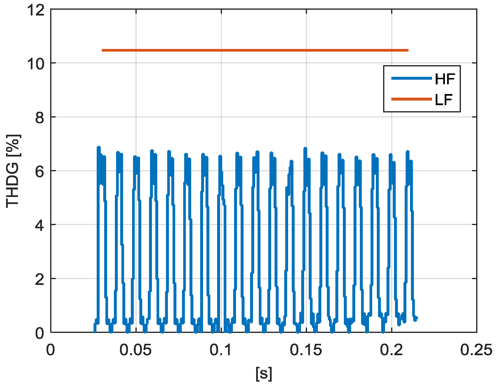
- and consider the energy of all of the spectral components in the spectrum, while and utilize the grouping of several harmonic orders, which do not include subharmonic and DC component information;
- the fundamental group at the denominators of and includes all of the spectral components from 25 Hz to 75 Hz, while and only consider the energy of the fundamental component;
- differently from and , there is not a total separation between the numerators of and , since, according to IEC standard [7], the last grouping of the low-frequency range and the first grouping of the high-frequency range have an overlap of 20 Hz.
4.2. Modern Non-Linear Loads
Case Study 4
4.3. Final Discussion on the Obtained Results
5. Conclusions
- (i)
- the short time disturbance energy index evaluated both for the low-frequency and high-frequency range ( and );
- (ii)
- the short time frequency deviation difference index evaluated both for the low-frequency and high-frequency distortions ( and );
- (iii)
- the short time k-factor difference index evaluated both for the low-frequency and high-frequency distortions ( and ).
Acknowledgments
Author Contributions
Conflicts of Interest
Appendix A
- (i)
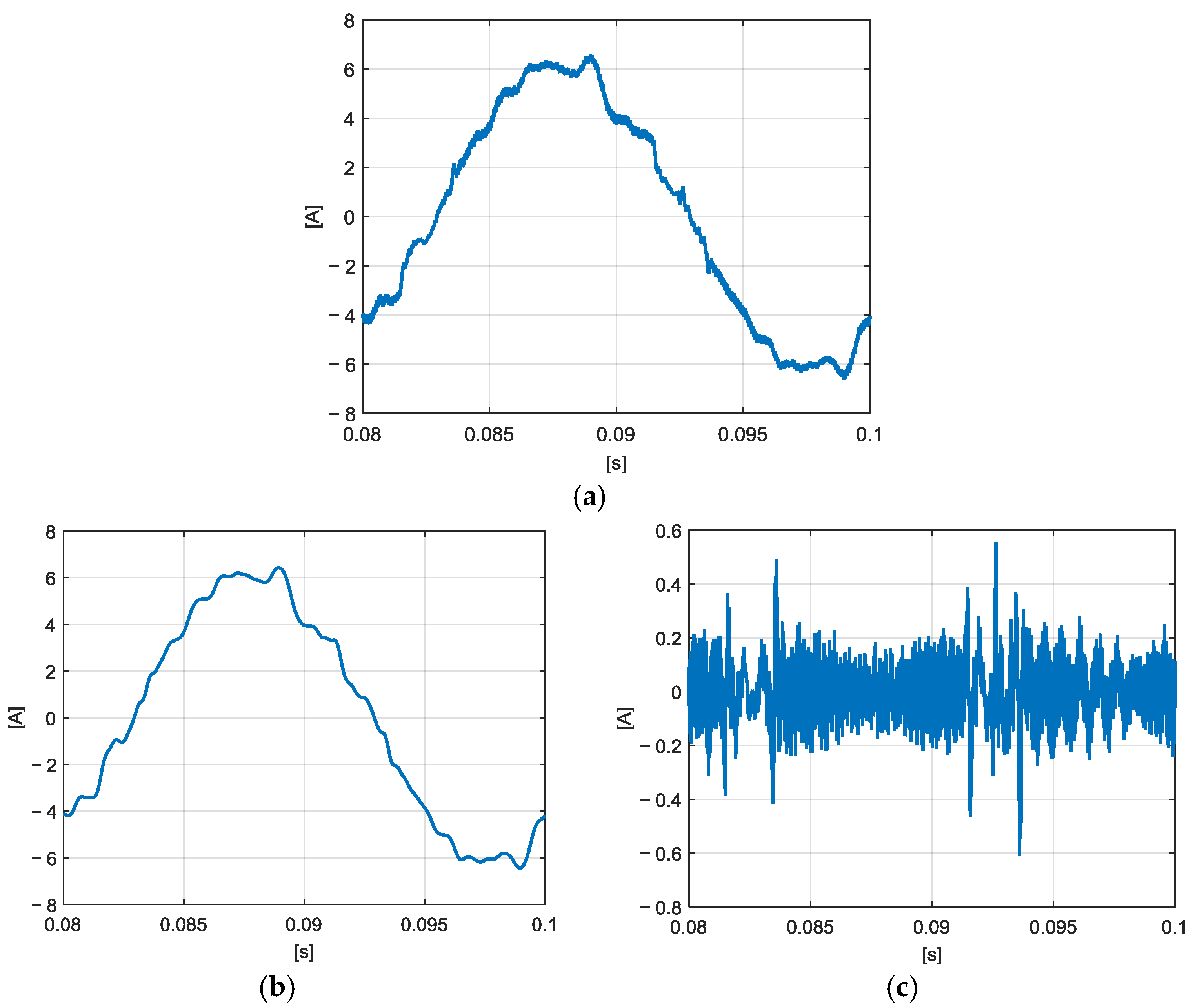
- in the first step, the original waveform to be analyzed is decomposed in a low-frequency waveform and in a high-frequency waveform by means of a discrete wavelet transform (DWT) [13];
- (ii)
- in the second step, the aforesaid two waveforms are properly resampled and analyzed separately by the sliding-window modified ESPRIT method (SW MEM) [27].
References
- Meyer, J.; Bollen, M.; Amaris, H.; Blanco, A.M.; Gil de Castro, A.; Desmet, J.; Klatt, M.; Kocewiak, Ł.; Rönnberg, S.; Yang, K. Future work on harmonics—Some expert opinions Part II—Supraharmonics standards and measurements. In Proceedings of the 16th IEEE International Conference on Harmonics and Quality of Power (ICHQP), Bucharest, Romania, 25–28 May 2014. [Google Scholar]
- International Council on Large Electrical Systems (CIGRE). Impact of Increasing Contribution of Dispersed Generation on the Power System; CIGRE WG 37–23; International Council on Large Electrical Systems (CIGRE): Paris, France, 1999. [Google Scholar]
- Ribeiro, P. Time-Varying Waveform Distortions in Power Systems; John Wiley & Sons: New York, NY, USA, 2009. [Google Scholar]
- Alfieri, L.; Bracale, A.; Carpinelli, G.; Larsson, A. A Wavelet-Modified ESPRIT Hybrid Method for Assessment of Spectral Components from 0 to 150 kHz. Energies 2017, 10, 97. [Google Scholar] [CrossRef]
- Moreno-Munoz, A.; Gil-de-Castro, A.; Romero-Cavadal, E.; Rönnberg, S.; Bollen, M. Supraharmonics (2 to 150 kHz) and multi-level converters. In Proceedings of the IEEE 5th International Conference on Power Engineering, Energy and Electrical Drives (POWERENG), Riga, Latvia, 11–13 May 2015; pp. 37–41. [Google Scholar]
- International Special Committee on Radio Interference. CISPR 15: Limits and Methods of Measurement of Radio Disturbance Characteristics of Electrical Lighting and Similar Equipment; International Special Committee on Radio Interference: Geneva, Switzerland, 2013. [Google Scholar]
- International Electrotechnical Commission (IEC). IEC Standard 61000–4-7: General Guide on Harmonics and Interharmonics Measurements, for Power Supply Systems and Equipment Connected Thereto; International Electrotechnical Commission (IEC): Geneva, Switzerland, 2010. [Google Scholar]
- International Electrotechnical Commission (IEC). IEC Standard 61000–4-30: Testing and Measurement Techniques—Power Quality Measurement Methods; International Electrotechnical Commission (IEC): Geneva, Switzerland, 2015. [Google Scholar]
- Larsson, E.O.A.; Bollen, M.H.J.; Wahlberg, M.G.; Lundmark, C.M.; Rönnberg, S.K. Measurements of high frequency (2–150 kHz) distortion in low-voltage networks. IEEE Trans. Power Deliv. 2010, 25, 1749–1757. [Google Scholar] [CrossRef]
- Bollen, M.; Olofsson, M.; Larsson, A.; Rönnberg, S.; Lundmark, M. Standards for supraharmonics (2 to 150 kHz). IEEE Electromagn. Compat. Mag. 2014, 3, 114–119. [Google Scholar] [CrossRef]
- Rönnberg, S.K.; Bollen, M.H.J.; Amaris, H.; Chang, G.W.; Gu, I.Y.H.; Kocewiak, Ł.H.; Meyer, J.; Olofsson, M.; Ribeiro, P.F.; Desmet, J. On waveform distortion in the frequency range of 2 kHz–150 kHz—Review and research challenges. Electr. Power Syst. Res. 2017, 150, 1–10. [Google Scholar] [CrossRef]
- Alfieri, L.; Bracale, A.; Carpinelli, G.; Larsson, A. Accurate Assessment of Waveform Distortions up to 150 kHz due to Fluorescent Lamps. In Proceedings of the 6th International Conference on Clean Electrical Power (ICCEP), Santa Margherita Ligure, Liguria, Italy, 27–29 June 2017. [Google Scholar]
- Caramia, P.; Carpinelli, G.; Verde, P. Power Quality Indices in Liberalized Markets; Wiley-IEEE Press: Chippenham, UK; Wiltshire, UK, 2009. [Google Scholar]
- Rönnberg, S.; Bollen, M. Power quality issues in the electric power system of the future. Electr. J. 2016, 29, 49–61. [Google Scholar] [CrossRef]
- Andreotti, A.; Bracale, A.; Caramia, P.; Carpinelli, G. Adaptive Prony Method for the Calculation of Power-Quality Indices in the Presence of Nonstationary Disturbance Waveforms. IEEE Trans. Power Deliv. 2009, 24, 874–883. [Google Scholar] [CrossRef]
- Shin, Y.; Powers, E.J.; Grady, M.; Arapostathis, A. Power quality indices for transient disturbances. IEEE Trans. Power Deliv. 2006, 21, 253–261. [Google Scholar] [CrossRef]
- Emanuel, A.; McEachern, A. Electric power definitions: A debate. In Proceedings of the IEEE Power & Energy Society (PES) General Meeting, Vancouver, BC, Canada, 21–25 July 2013. [Google Scholar]
- Larsson, E.O.A.; Bollen, M.H.J. Measurement result from 1 to 48 fluorescent lamps in the frequency range 2 to 150 kHz. In Proceedings of the 14th International Conference on Harmonics and Quality of Power (ICHQP), Bergamo, Italy, 26–29 September 2010; pp. 1–8. [Google Scholar]
- Yazdani, A.; Di Fazio, A.R.; Ghoddami, H.; Russo, M.; Kazerani, M.; Jatskevich, J.; Strunz, K.; Leva, S.; Marinez, J.A. Modeling guidelines and a benchmark for power system simulation studies of three-phase single-stage photovoltaic systems. IEEE Trans. Power Deliv. 2011, 26, 1247–1264. [Google Scholar] [CrossRef]
- Renner, H.; Heimbach, B.; Desmet, J. Power quality and electromagnetic compatibility: Special report session 2. In Proceedings of the 23rd International Conference and Exhibition on Electricity CIRED, Lyon, France, 15–18 June 2015. [Google Scholar]
- Li, H.; Chen, Z. Overview of different wind generator systems and their comparisons. IET Renew. Power Gener. 2008, 2, 123–138. [Google Scholar] [CrossRef]
- Blaabjerg, F.; Iov, F.; Chen, Z.; Ma, K. Power electronics and controls for wind turbine systems. In Proceedings of the 2010 IEEE International Energy Conference and Exhibition (EnergyCon), Manama, Bahrain, 18–22 December 2010. [Google Scholar]
- Alfieri, L. Some advanced parametric methods for assessing waveform distortion in a smart grid with renewable generation. EURASIP J. Adv. Signal Process. 2015, 2015, 1–16. [Google Scholar] [CrossRef]
- Bracale, A.; Caramia, P.; Carpinelli, G.; Di Fazio, A.R. Modeling the three-phase short-circuit contribution of photovoltaic systems in balanced power systems. Int. J. Electr. Power Energy Syst. 2017, 93, 204–215. [Google Scholar] [CrossRef]
- Bracale, A.; Caramia, P.; Carpinelli, G.; Rapuano, A. A New, Sliding-Window Prony and DFT Scheme for the Calculation of Power-Quality Indices in the Presence of Non-stationary Waveforms. Int. J. Emerg. Electr. Power Syst. 2012, 13, 112–120. [Google Scholar] [CrossRef]
- Gallo, D.; Landi, C.; Luiso, M. AC and DC power quality of photovoltaic systems. In Proceedings of the IEEE International Instrumentation and Measurement Technology Conference (I2MTC), Graz, Austria, 13–16 May 2012; pp. 576–581. [Google Scholar]
- Alfieri, L.; Carpinelli, G.; Bracale, A. New ESPRIT-based method for an efficient assessment of waveform distortions in power systems. Electr. Power Syst. Res. 2015, 122, 130–139. [Google Scholar] [CrossRef]


© 2017 by the authors. Licensee MDPI, Basel, Switzerland. This article is an open access article distributed under the terms and conditions of the Creative Commons Attribution (CC BY) license (http://creativecommons.org/licenses/by/4.0/).
Share and Cite
Alfieri, L.; Bracale, A.; Larsson, A. New Power Quality Indices for the Assessment of Waveform Distortions from 0 to 150 kHz in Power Systems with Renewable Generation and Modern Non-Linear Loads. Energies 2017, 10, 1633. https://doi.org/10.3390/en10101633
Alfieri L, Bracale A, Larsson A. New Power Quality Indices for the Assessment of Waveform Distortions from 0 to 150 kHz in Power Systems with Renewable Generation and Modern Non-Linear Loads. Energies. 2017; 10(10):1633. https://doi.org/10.3390/en10101633
Chicago/Turabian StyleAlfieri, Luisa, Antonio Bracale, and Anders Larsson. 2017. "New Power Quality Indices for the Assessment of Waveform Distortions from 0 to 150 kHz in Power Systems with Renewable Generation and Modern Non-Linear Loads" Energies 10, no. 10: 1633. https://doi.org/10.3390/en10101633
APA StyleAlfieri, L., Bracale, A., & Larsson, A. (2017). New Power Quality Indices for the Assessment of Waveform Distortions from 0 to 150 kHz in Power Systems with Renewable Generation and Modern Non-Linear Loads. Energies, 10(10), 1633. https://doi.org/10.3390/en10101633