1. Introduction
Solar forecasts are required to increase the penetration of solar power into electricity grids. Accurate forecasts are important for several tasks. They can be used to ensure the balance between supply and demand necessary for grid stability [
1]. At more localized scales, solar forecasts are used to optimize the operational management of grid-connected storage systems associated with intermittent solar resource [
2].
A proper assessment of uncertainty estimates enables a more informed decision-making processes, which in turn, increases the value of solar power generation. Thus, a point forecast plus a prediction interval provide more useful information than simply the point forecast and are essential to increase the penetration of solar energy into the electrical grids. Given the recognized value of accurate probabilistic solar forecast, this work proposes techniques to improve their quality and performance.
Some recent works dealt with intra-day or intra-hour solar probabilistic forecasting. Grantham et al. [
3] proposed a non-parametric approach based on a specific bootstrap method to build predictive global horizontal solar irradiance (GHI) distributions for a forecast horizon of 1 h. Chu and Coimbra [
4] developed models based on the k-nearest-neighbors (kNN) algorithm for generating very short-term (from 5 min–20 min) direct normal solar irradiance (DNI) probabilistic forecasts. Golestaneh et al. [
5] used an extreme machine learning method to produce very short-term PV power predictive densities for lead times between a few minutes to one hour ahead. David et al. [
6] used a parametric approach based on a combination of two linear time series model (ARMA-GARCH) to generate 10 min–6 h GHI probabilistic forecasts using only past ground data.
In a previous study, Lauret et al. [
7] demonstrated that intra-day point deterministic forecasts can be improved by considering both past ground measurements and day-ahead ECMWF forecasts in the set of predictors.
In this work, it is investigated if such a combination could also improve the quality of the probabilistic forecasts. In order to test this conjecture, we build three probabilistic models based on the linear quantile regression method. The first model uses the deterministic point prediction generated by a linear model as unique explanatory input variable. The second one only makes use of past solar ground measurements, while the third one combines past ground data with exogenous inputs. These consist, as mentioned, of forecasted data obtained from the Integrated Forecast System (IFS) Numerical Weather Prediction (NWP) model [
8].
Once the models are trained and applied to the testing set, we analyze the quality of the probabilistic forecasts using several qualitative and quantitative tools: reliability diagrams [
9], the rank histograms (or Talagrand histograms) [
10] and the continuous ranked probability score (CRPS) [
11]. We will also assess the sharpness of the predictive distributions by calculating the prediction intervals normalized average width (PINAW) [
12,
13].
The remainder of this paper is organized as follows:
Section 2 provides information about the locations studied, the data collection and data preprocessing.
Section 3 analyzes the solar irradiance variability observed at the two locations under study.
Section 4 describes the exogenous data collected from the ECMWF forecasts.
Section 5 presents the different probabilistic models based on the quantile regression method.
Section 6 details the different metrics used to evaluate the quality of the solar probabilistic forecasts, and
Section 7 presents the results based on the evaluation framework.
Section 8 discusses the impact of the sky conditions on the quality of the predictive distributions. Finally,
Section 9 gives some concluding remarks.
2. Data
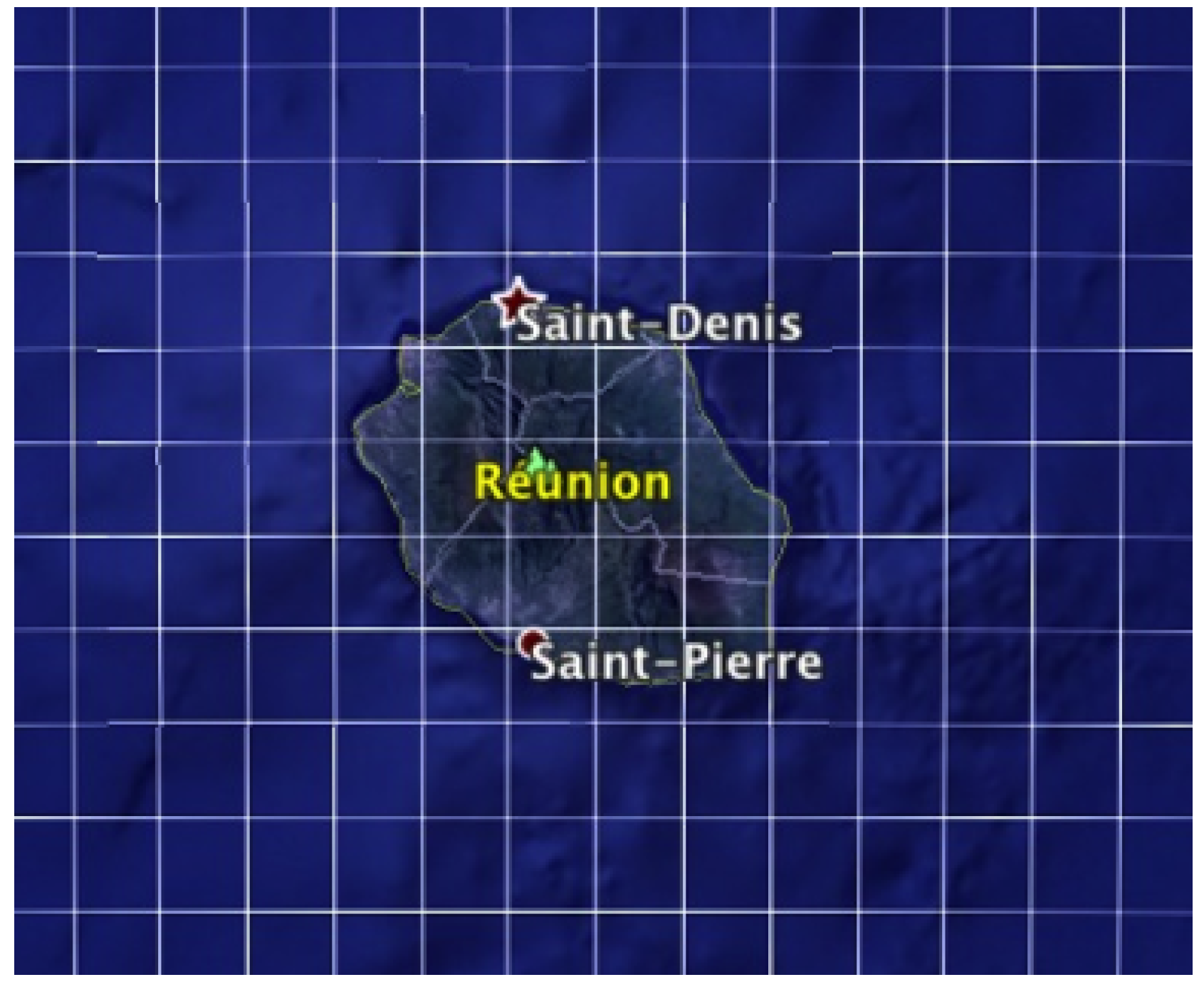
In this paper, we used two consecutive years of 1-min data collected at two sites that exhibit completely different sky conditions. The first site (Le Tampon) is located on La Réunion Island and experiences variable sky conditions, while the second one is situated in the continental U.S. and experiences an arid climate (Desert Rock).
Table 1 lists the characteristics of the two sites. For this study, we computed 1-h averages of global horizontal solar irradiance (GHI) directly from the raw 1 min-data. The first year (2012) constitutes the training dataset used to build the forecasting models. The second year (2013) was used to evaluate the probabilistic forecasts (testing or evaluation dataset).
Solar irradiance is characterized by deterministic diurnal and seasonal variations. Such a component can be removed from the analysis by working with the clear sky index (
) instead of the original GHI time series, where
is defined as:
This quantity corresponds to the ratio of the measured GHI
to the theoretical GHI observed under clear sky
. This preprocessing technique separates the geometric and the deterministic component of GHI from the stochastic component that is related to the cloud cover. The target variable for the forecasting model is then the stochastic component. Here, we used the clear sky data provided by the McClear model [
14] publicly available on the Solar radiation Data (SoDa) website [
15]. This model uses aerosol optical depth, water vapor and ozone data from the MACC (Monitoring Atmospheric Composition and Climate) project [
16].
Finally, data points corresponding to nighttime and low solar elevations (solar zenith angle greater than 85) were discarded from the dataset. This filtering removes less than 1% of the total annual sum of solar energy and discards measurements with large uncertainty (uncertainties associated with pyranometers are typically much higher than 3.0% for ).
Notice that, in addition to the filtering based on the zenith angle, a specific procedure was also used to preprocess the GHI data. This procedure is described at length in [
6].
3. Site Analysis
Figure 1 plots the clear sky index distribution of each location. As shown by
Figure 1, the continental station of Desert Rock experiences weather dominated by clear skies, evidenced by the high frequency of
near one. For the insular location Le Tampon, the occurrence of clear skies is much lower. In
Figure 1, one can notice a significant number of occurrences of the clear sky index above one. These events result from a phenomenon known as the cloud edge effect and can be observed anywhere in the world [
17,
18].
Table 1 (last row) lists the solar variability of each site. This quantity is calculated as the the standard deviation of step changes in the clear sky index
[
19]. This metric was computed for hourly
values (
= 1 h) for the whole dataset (two years). The application of this metric to other locations [
19] led to the conclusion that variability above 0.2 indicates very unstable GHI conditions. As the table indicates, variability for Le Tampon is above this threshold.
In [
7], it was demonstrated that point deterministic forecasts for insular sites like Le Tampon are prone to have worse forecasting performance than less variable (continental or insular) sites. This fact results from the higher solar variability resulting from local cloud formation and dissipation.
Section 8 below discusses the impact of the site variability on the forecasting performance of the different probabilistic models.
At this point, it must be stressed that the site of Desert Rock is only used to address the impact of the sky conditions on the quality of the probabilistic forecasts.
5. Probabilistic Models
In this study, we make no assumption about the shape of the predictive distributions. Consequently, the probabilistic forecasts are produced by non-parametric methods like quantile regression. In other words, the predictive distributions are defined by a number of quantile forecasts with nominal proportions spanning the unit interval [
21].
In this work, we chose to use the simple linear quantile regression (QR) method proposed by [
22] in order to build the probabilistic models. It must be stressed that possibly better results can be obtained with more sophisticated machine learning methods like quantile regression forest [
23], QR neural networks [
24] or gradient boosting techniques [
25]. However, our goal here is to focus on the combination of ground telemetry and ECMWF forecasts, as well as the impact on the sky conditions experienced by a site on the quality of the probabilistic forecasts.
5.1. The Linear Quantile Regression Method
This method estimates the quantiles of the cumulative distribution function of some variable
y (also called the predictand) by assuming a linear relationship between
y and a vector of explanatory variables (also called predictors)
:
where
is a vector of parameters to optimize and
represents a random error term.
In quantile regression, quantiles are estimated by applying asymmetric weights to the mean absolute error. Following [
22], the quantile loss function is:
with
representing the quantile probability level.
The quantity
is the
quantile estimated by the quantile regression method with the vector
obtained as the solution of the following minimization problem:
where
denotes a pair of vector of predictors and the corresponding observed predictand in the training set.
It must be noted that the quantile regression method estimates each quantile separately (i.e., the minimization of the quantile loss function is made for each
separately). As a consequence, one can obtain quantile regression curves that may intersect, i.e.,
when
. To avoid this issue during the model fitting, we used the rearrangement method described by [
26].
In the following, the predictand
y is the clear sky index
. Therefore, the output of the probabilistic model for each forecasting time horizon
h is the ensemble of nine quantiles defined by
for each forecasting time horizon
h = 1, ⋯, 6 h. This set of
quantiles can be transformed into GHI quantiles
by using Equation (
1). As mentioned above, this set of quantiles represents the predictive distribution of the target variable (here GHI) at lead time
. This set of quantiles may form also what the verification weather community [
27] calls an ensemble prediction system (EPS).
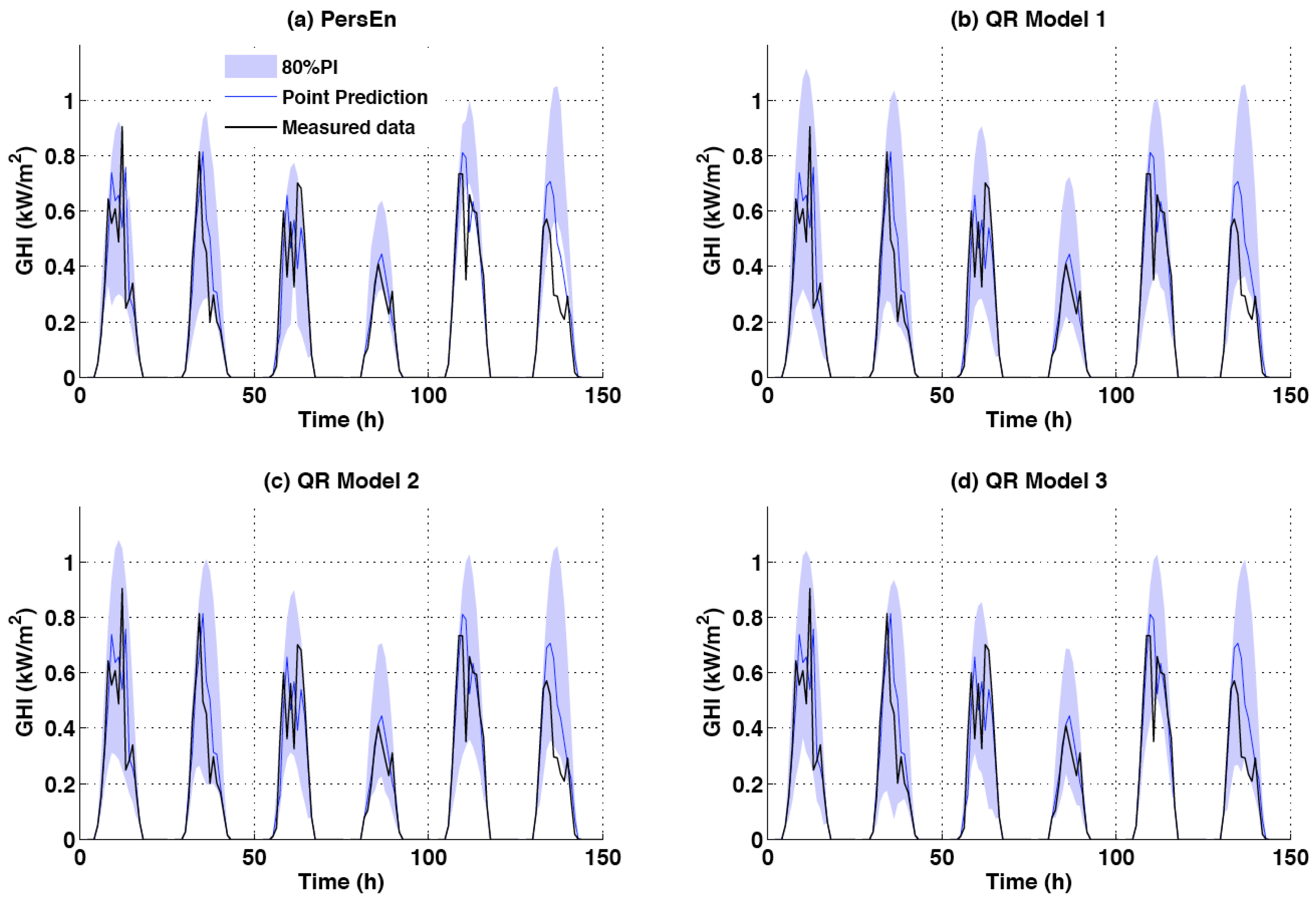
In addition, prediction intervals with different nominal coverage rates can be inferred from this set of quantiles. These intervals provide lower and upper bounds within which the true value of GHI is expected to lie with a probability equal to the prediction interval’s nominal coverage rate. In this work, the
central prediction interval is generated by taking the
quantile as the lower bound and the
quantile as the upper bound. More precisely, a prediction interval with a
nominal coverage rate produced at time
t for lead time
is defined by:
For instance, a is calculated from the two extremes quantiles of the forecasted irradiance distribution, i.e., and .
5.2. QR Model 1: Point Forecast as Unique Explanatory Variable
In this simple setup, the deterministic point forecast produced by a simple linear auto-regressive moving average (ARMA) model constitutes the unique explanatory variable of the QR model. Therefore, we have:
Indeed, in a study related to solar power forecasting, Bacher et al. [
28] showed that the level of uncertainty depends on the value of the point forecast. The detailed description of this ARMA model can be found at [
6].
5.3. QR Model 2: Past Ground Measurements Only
For this model, the vector of explanatory variables consists of the six past ground measurements, i.e.,
5.4. QR Model 3: Combination of Past Ground Measurements Plus ECMWF Forecast Data
The third QR model developed in this work considers as predictors the six past ground measurements plus exogenous data provided by the day-head ECMWF forecasts. As explained above in
Section 4, the exogenous data consists of the forecasted clear sky index
and the total cloud cover
predicted for time
. With these data, the vector of predictors is given by:
The selection of exogenous data follows a previous work [
7] regarding point deterministic forecasts. There, it was shown that forecasts with improved accuracy can be obtained if one adds total cloud cover (TCC) as an explanatory variable.
5.5. Persistence Ensemble Model
Finally, we define the simple baseline persistence ensemble model (PersEn). This model [
4,
6,
29] is commonly used to provide reference probabilistic forecasts. In this work, the PersEn considers the GHI lagged measurements in the 10 h that precede the forecasting issuing time. The selected measurements are ranked to define quantile values for the irradiance forecast.
6. Probabilistic Error Metrics
In [
21], the authors emphasize several aspects related to the quality of a probabilistic forecasting system namely reliability, sharpness and resolution. These required properties for skillful probabilistic forecasts possess different meanings according a meteorologist’s point of view or a statistician’s point of view. The interested reader is referred to [
30,
31] for a definition of these properties in the realm of meteorology. As an illustration of these different definitions, the meteorological literature [
30] defines the sharpness property as the ability of the forecasting system to produce forecasts that are able to deviate from the climatological value of the predictand while from a statistical point of view (as will be the case here), the sharpness property refers to the concentration of the predictive distributions [
12,
21].
The main requirement when studying the performance of probabilistic forecasts is reliability. As noted in [
21], the lack of reliability introduces systematic bias that affects negatively the subsequent decision-making process. A reliable EPS is said to be calibrated. More precisely, a probabilistic forecasting system is reliable if, statistically, the nominal proportions of the quantile forecasts are equal to the proportions of the observed value. In other words, over a testing set of significant size, the difference between observed and nominal probabilities should be as small as possible. This first requirement of reliability will be assessed with the help of reliability diagrams (see
Section 6.1.1) or by calculating the prediction interval coverage probability (PICP) [
13] (see
Section 6.1.2), which permits one to assess the reliability of the forecasts in terms of coverage rate. As a means to corroborate the analysis made with the reliability diagram, we will also provide rank histograms (see
Section 6.1.3) that allow judging the statistical consistency of the ensemble constituted by the nine quantiles’ members.
In this work, and similarly to [
12,
21], the assessment of sharpness derives from a more statistical point of view with focus on the shape of the predictive distributions. For that purpose, the prediction interval average width (PINAW) metric (see
Section 6.2) is used to evaluate the sharpness of the predictive distributions [
13].
Regarding the third property, namely resolution, it consists of evaluating the ability of the forecast system to issue different probabilistic forecasts (i.e., predictive distributions with prediction intervals that vary in size) depending on the forecast conditions [
21]. For instance, in the case of GHI, the level of uncertainty may vary according the Sun’s position in the sky (see for the instance the work of [
3]). In this paper, however, we will not provide such a conditional assessment and will only focus on the most important properties of a skillful prediction system, namely reliability and sharpness.
Finally, it must be noted that reliability can be corrected by statistical techniques also called calibration techniques [
32], whereas the same is not possible for sharpness. Finally, the continuous rank probability score (CRPS) [
11] provides an evaluation of the global skill of our probabilistic models.
6.1. Reliability Property
6.1.1. Reliability Diagram
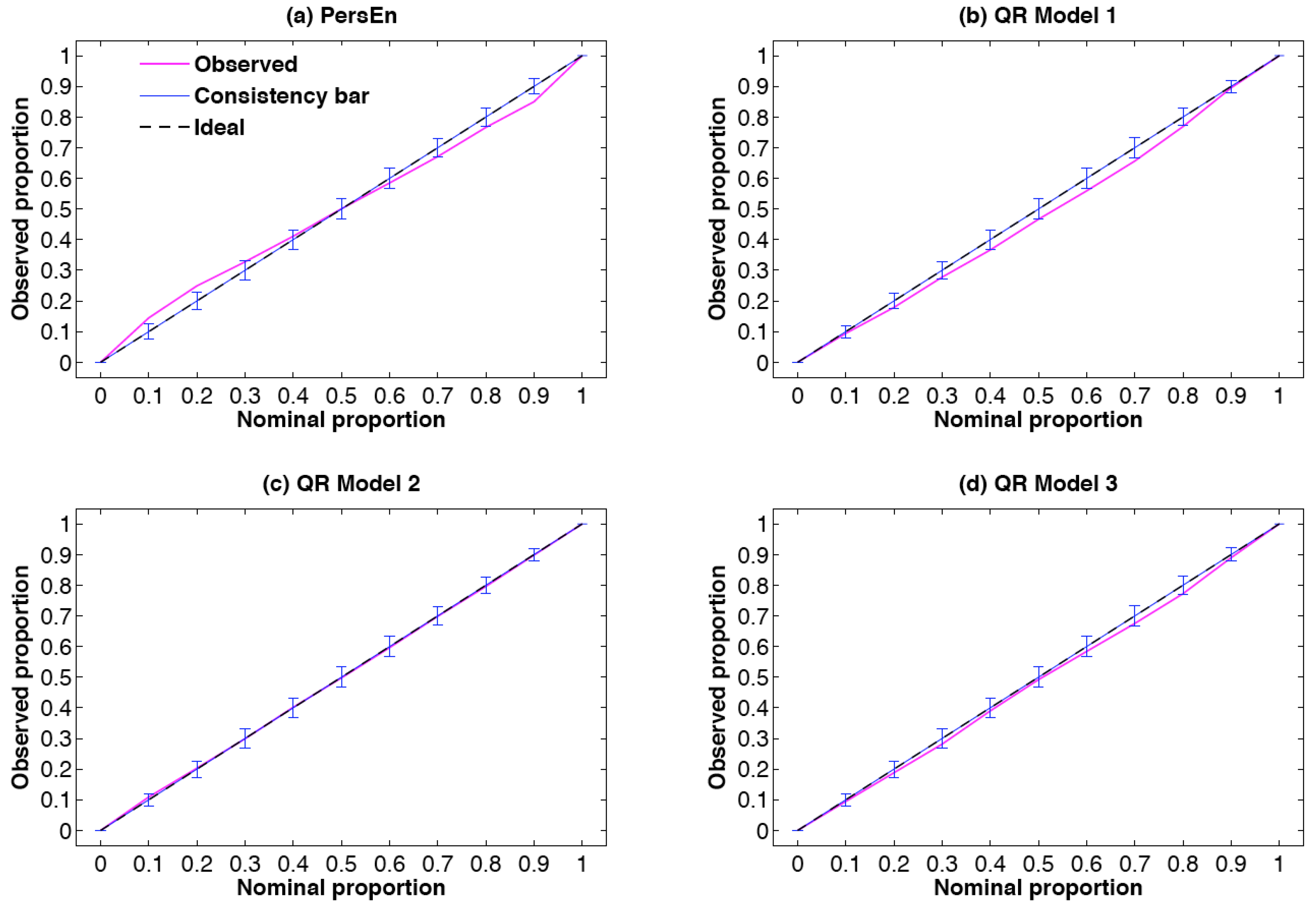
The reliability diagram is a graphical verification display used to verify the reliability component of a probabilistic forecast system. In this work, we use the methodology defined by [
9] that is especially designed for density forecasts of continuous variables.
This type of reliability diagram plots the observed probabilities against the nominal ones (i.e., the probability levels of the different quantiles). By doing so, deviations from perfect reliability (the diagonal) are immediately revealed in a visual manner [
9]. However, due to the finite number of pairs of observation/forecast and also due to possible serial correlation in the sequence of forecast-verification pairs, it is not expected that observed proportions lie exactly along the diagonal, even if the density forecasts are perfectly reliable [
9]. In this work, similarly to [
33], consistency bars are computed in order to take into account the limited number of observation/forecast pairs of the evaluation (testing) set.
6.1.2. PICP
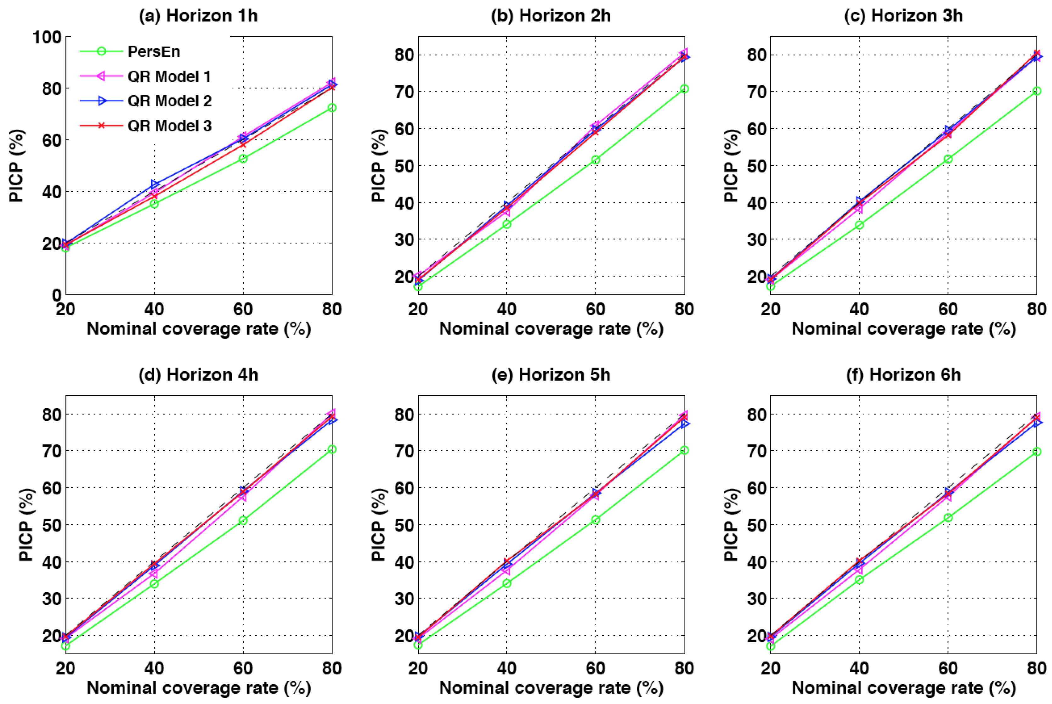
The prediction interval coverage probability (PICP) [
13] is a metric that permits one to assess the reliability of the EPS in terms of coverage rate. In addition, and contrary to what we did for reliability diagram, here we assess the PICP as a function of the forecast horizon. In this work, and as mentioned above, we propose to assess the empirical coverage probability of the central prediction intervals for a different nominal coverage rate
. Equation (
9) gives the definition of the PICP for a specific forecast horizon
h and a particular nominal coverage rate:
The indicator function has the value of one if its argument u is true and zero otherwise.
6.1.3. Rank Histogram
The rank histogram [
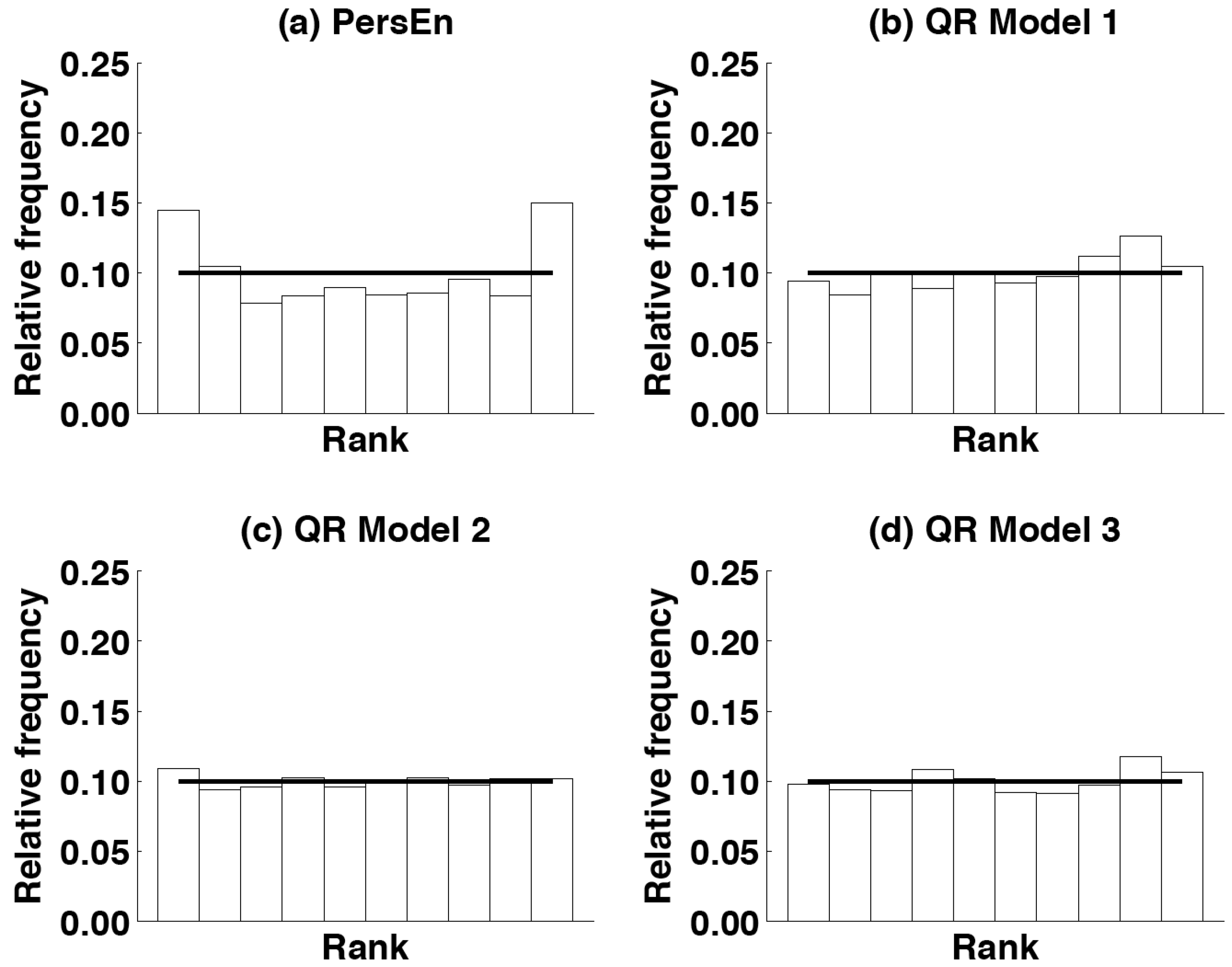
30] is another graphical tool for evaluating ensemble forecasts. Rank histograms are useful for determining the statistical consistency of the ensemble, that is if the observation being predicted looks statistically just like another member of the forecast ensemble [
30]. A necessary condition for ensemble consistency is an appropriate degree of ensemble dispersion leading to a flat rank histogram [
30]. If the ensemble dispersion is consistently too small (underdispersed ensemble), then the observation (also called the verification sample) will often be an outlier in the distribution of ensemble members. This will result in a rank histogram with a U-shape. Conversely, if the ensemble dispersion is consistently too large (overdispersed ensemble), then the observation may too often be in the middle of the ensemble distribution. This will give a rank histogram with a hump shape. In addition, asymmetric rank histograms may suggest that the ensemble may possess some biases. Ensemble bias can be detected from overpopulation of either the smallest ranks, or the largest ranks, in the rank histogram. An over-forecasting bias will correspond to an overpopulation of the smallest ranks, while an under-forecasting bias will overpopulate the highest ranks. As a consequence, rank histograms can also reveal deficiencies in ensemble calibration or reliability [
30]. Again, care must be taken when analyzing rank histograms when the number of verification samples is limited. In addition, as demonstrated by [
10], a perfect rank histogram does not mean that the corresponding EPS is reliable.
To obtain a verification rank histogram, one needs to find the rank of the observation when pooled within the ordered ensemble of quantile values and then plot the histogram of the ranks. For a number of members M, the number of ranks of the histogram of an ensemble is . If the consistency condition is met, this histogram of verification ranks will be uniform with a theoretical relative frequency of .
6.2. Sharpness
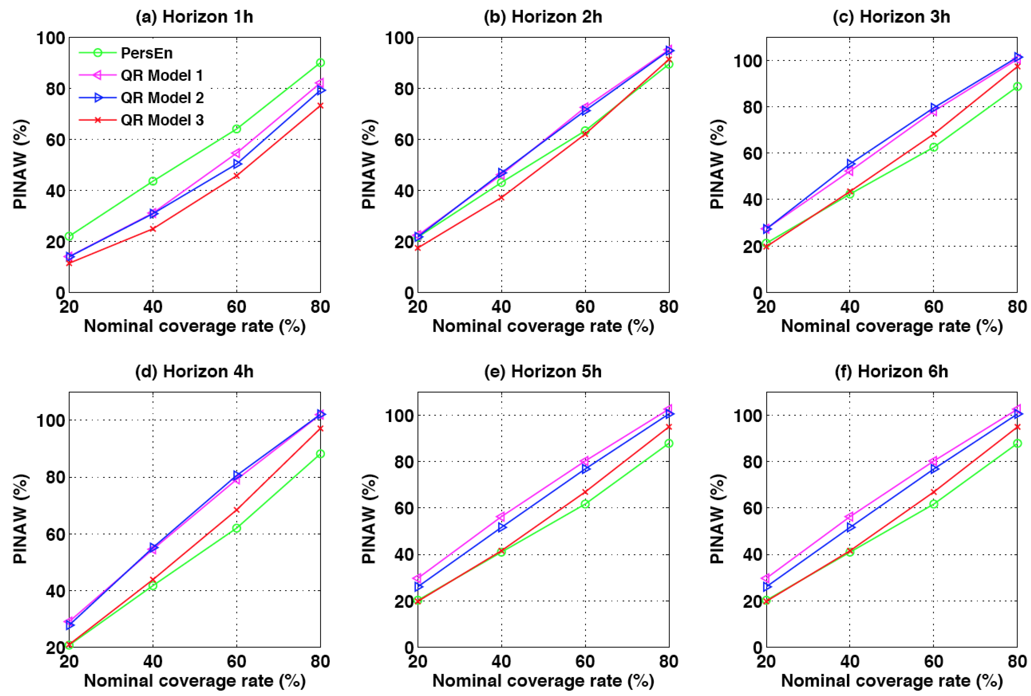
Sharp probabilistic forecasts must present prediction intervals that are shorter on average than the ones derived from naive methods, such as climatology or persistence. The prediction interval normalized averaged width (PINAW) is related to the informativeness of PIs or equivalently to the sharpness of the predictions. As for the PICP, we assess the sharpness of the forecasts by calculating the PINAW for different nominal coverage rates
. More precisely, this metric is the average width of the
prediction interval normalized by the mean of GHI for the testing set. Equation (
10) gives the definition of the PINAW metric for lead time
h and for a specific nominal coverage rate.
As mentioned in [
12], the objective of any probabilistic forecasting model is to maximize the sharpness of the predictive distributions (minimize PINAW) while maintaining a coverage rate (PICP) close to its nominal value.
6.3. CRPS
The CRPS quantifies deviations between the cumulative distributions functions (CDF) for the predicted and observed data. The formulation of the CRPS is:
where
is the predictive CDF of the variable of interest
x (here GHI) and
is a cumulative-probability step function that jumps from zero to one at the point where the forecast variable
x equals the observation
(i.e.,
). The squared difference between the two CDFs is averaged over the
N ensemble forecast/observation pairs. The CRPS has the same dimension as the forecasted variable. The CRPS is negatively oriented (smaller values are better), and it rewards the concentration of probability around the step function located at the observed value [
30]. Thus, the CRPS penalizes the lack of sharpness of the predictive distributions, as well as biased forecasts.
Similarly to the forecast skill score commonly used to assess the quality of point forecasts, we also include the CRPSS (for continuous rank probability skill score). The latter (in %) is given by:
where
is the CRPS for the persistence ensemble model and
is the CRPS for the model
m (here the QR models). Negative values of CRPSS indicate that the probabilistic method fails to outperform the persistence ensemble model, while positive values of CRPSS mean that the forecasting method improves on persistence ensemble. Further, the higher the CRPSS score, the better the improvement.
8. Impact of Data Variability on the Quality of the Probabilistic Forecasts
In this section, we study the impact of local sky conditions (as quantified by the site variability listed in
Table 1) on the forecast performance.
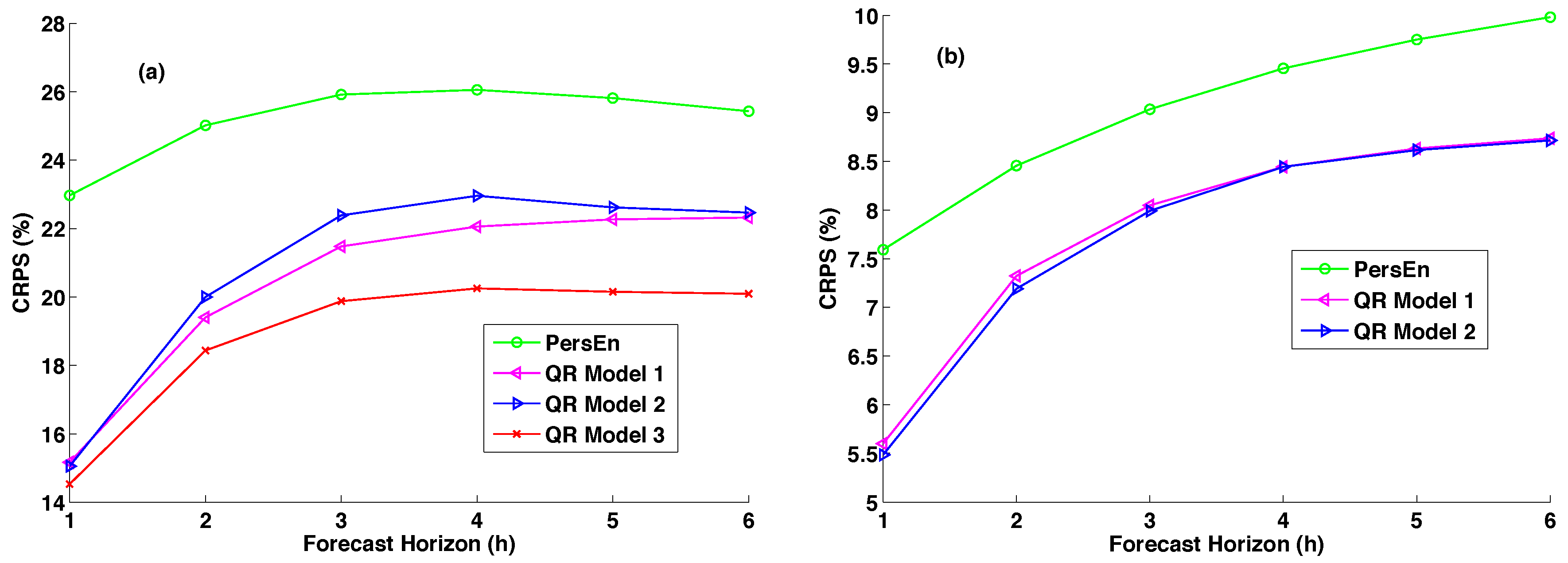
Table 3 gives the CRPS together with the CRPSS of the different models (except QR Model 3) for the site of Desert Rock. As we have seen, this location displays low annual variability and a high frequency of clear skies (
).
As shown by
Table 3, the performance of the models in terms of CRPS is obviously better for the site of Desert Rock than for the Le Tampon site. Indeed, for this site, the CRPS values for the QR models range from 30 W·m
to 48 W·m
, which translates into 5.5–8.7% for the relative counterparts (see also
Figure 8b). Again, the skill scores of the QR models demonstrate that these techniques outperform the reference PersEn model regardless of the site under study and the corresponding irradiance variability.
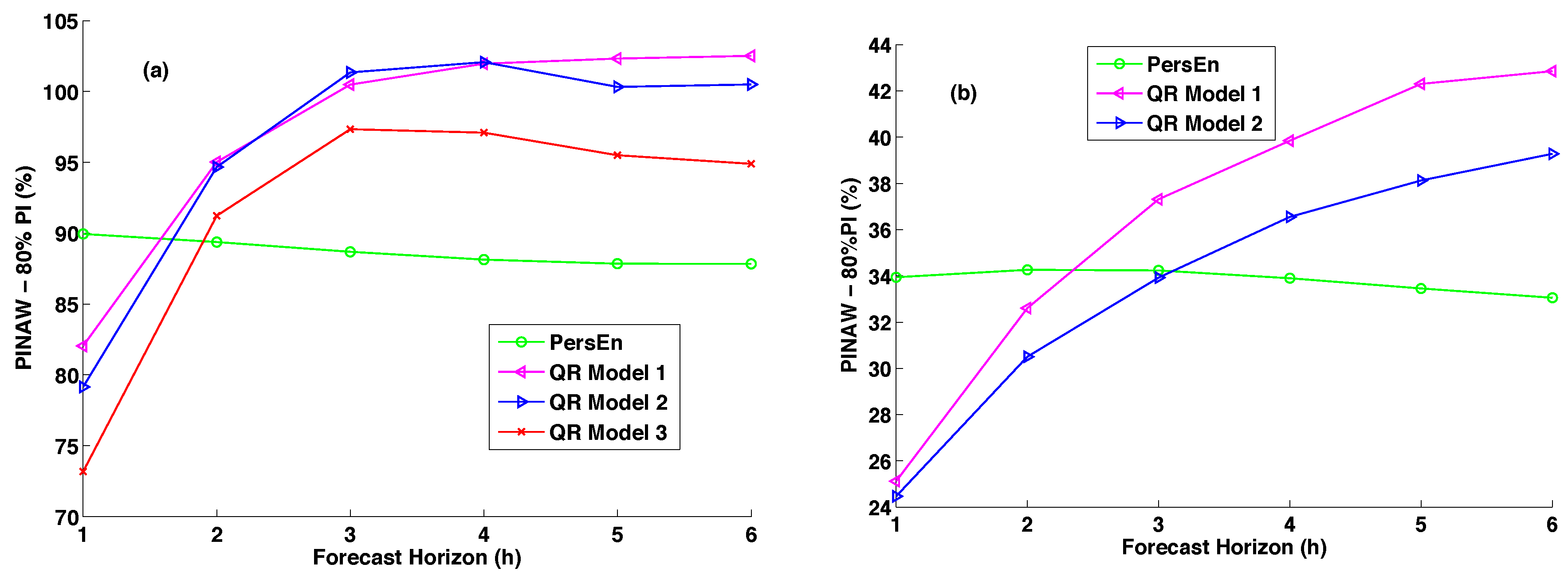
Figure 7b shows the PINAW values for the 80% nominal coverage rate obtained for the site of Desert Rock. Here, PINAWs for the two QR models lie between 24% and 42%, which correspond to prediction intervals’ width between 131 W·m
and 230 W·m
. Let us recall that for Le Tampon site, the corresponding values were 341 W·m
and 455 W·m
. This comparison confirms that the sky conditions have a clear impact on the forecasting quality of the probabilistic models.
Based on a previous study [
6], we can conjecture a link between the typology of the solar irradiance experienced by a site (i.e., distribution of the clear sky index and variability) and the performance of the probabilistic models. An in-depth study with more sites (>2) is needed to establish definitively a link between solar variability and the performance of the probabilistic models.


