1. Introduction
The connection of nonlinear loads to the ac grid becomes in non desirable effects such as grid harmonics. The main task of a shunt active power filter is to compensate such harmonics, and as a consequence to reduce, as much as possible, the total harmonic distortion (THD) of the currents injected to the grid [
1]. Different methods have been presented in the past in order to improve the grid power quality, such as passive filters or active power filters [
2,
3,
4]. Usually, the use of passive power filters to suppress the current harmonics has been considered in the past due to their low cost. Nevertheless, the sensitive to system parameters variation become in a resonance problem in these kind of filters. Conversely, shunt active power filters (SAPFs) can be used to overcome the aforementioned problems. In contrast to passive power filters, SAPFs are a flexible solution to compensate current harmonics generated by different types of non-linear loads. Nevertheless, the control of a SAPF is a challenging control problem since a high control bandwidth is required.
Several techniques addressed to control these kind of power converters have been presented in the literature, such as sliding mode control (SMC) [
3], optimal control [
5] and model predictive control (MPC) [
6,
7,
8]. Currently, and thanks to the potential of digital signal processors (DSPs), the MPC is a promising control method and has several benefits such as fast tracking response, a high control bandwidth and a very easiest way to include system nonlinearities and constraints [
9].
Two different control strategies regarding the MPC algorithms can be adopted: Continuous Control Set Model Predictive Control (CCS-MPC) and Finite Control Set Model Predictive Control (FCS-MPC). The former is based on the prediction of the sate variables according to a discrete model of the converter. These predictions are evaluated in a cost function over a prediction horizon in order to obtain a sequence of the future control actions. Then, only the first value of this sequence is considered and the algorithm is computed in each sampling period. This approach has several advantages such as an improvement of the THD, and the fixed switching frequency. However, a high amount of calculations are needed in order to solve the cost function which makes this option a more complex solution. In the latter, the optimization problem is reduced to a finite number of switching states. Here, the cost function is calculated for every switching state, each one related to a specific voltage vector. The switching state that minimizes the error between the current and its reference is then applied to the converter. In this way, the cost function is evaluated in a finite number of times for each sampling period.
FCS-MPC has been applied as a new method to control power converters [
10,
11,
12]. As a difference with other techniques such as PI or PR controllers, this control method is characterized by a direct drive of the inverter switches without the use of PWM-based techniques. To do this, the optimum voltage vector is selected according to an specific cost function minimization.
An interesting feature of this control strategy is the very fast transient response and a similar control bandwidth as the SMC technique. Another attractive performance is the possibility to include some restrictions due to the flexible nature of the cost function. In general terms, the number of voltage vectors can be larger than the number of switching states. Therefore, the main goal is to reduce the number of computations by eliminating some vectors according to some specific conditions. For instance in [
13] the SMC technique is used as a pre-selection task. In this case, the attractive conditions are used to decide which voltage vectors can be considered.
This paper proposes a combination of the vector operation technique with FCS-MPC in order to reduce the number of voltage vectors. The main advantage of combining both techniques is that for each region the number of possible voltage vectors to be considered can be reduced to a half, thus reducing the computational load employed by the control algorithm. Besides, in each region, only two phase-legs are switching at high frequency while the remaining phase-leg is maintained to a constant dc-voltage value during this interval. Accordingly, a reduction of the switching losses is obtained. Unlike the usual prediction techniques, a Kalman filter (KF) is used to predict the voltage and current of the SAPF. This solution provides high robustness against system parameters deviations and noise. The main advantage of this method is that the reference current is generated from the estimated voltages at the point of common coupling (PCC) in order to obtain the reference currents without any distortion, even in case of a highly distorted grid.
2. System Modeling
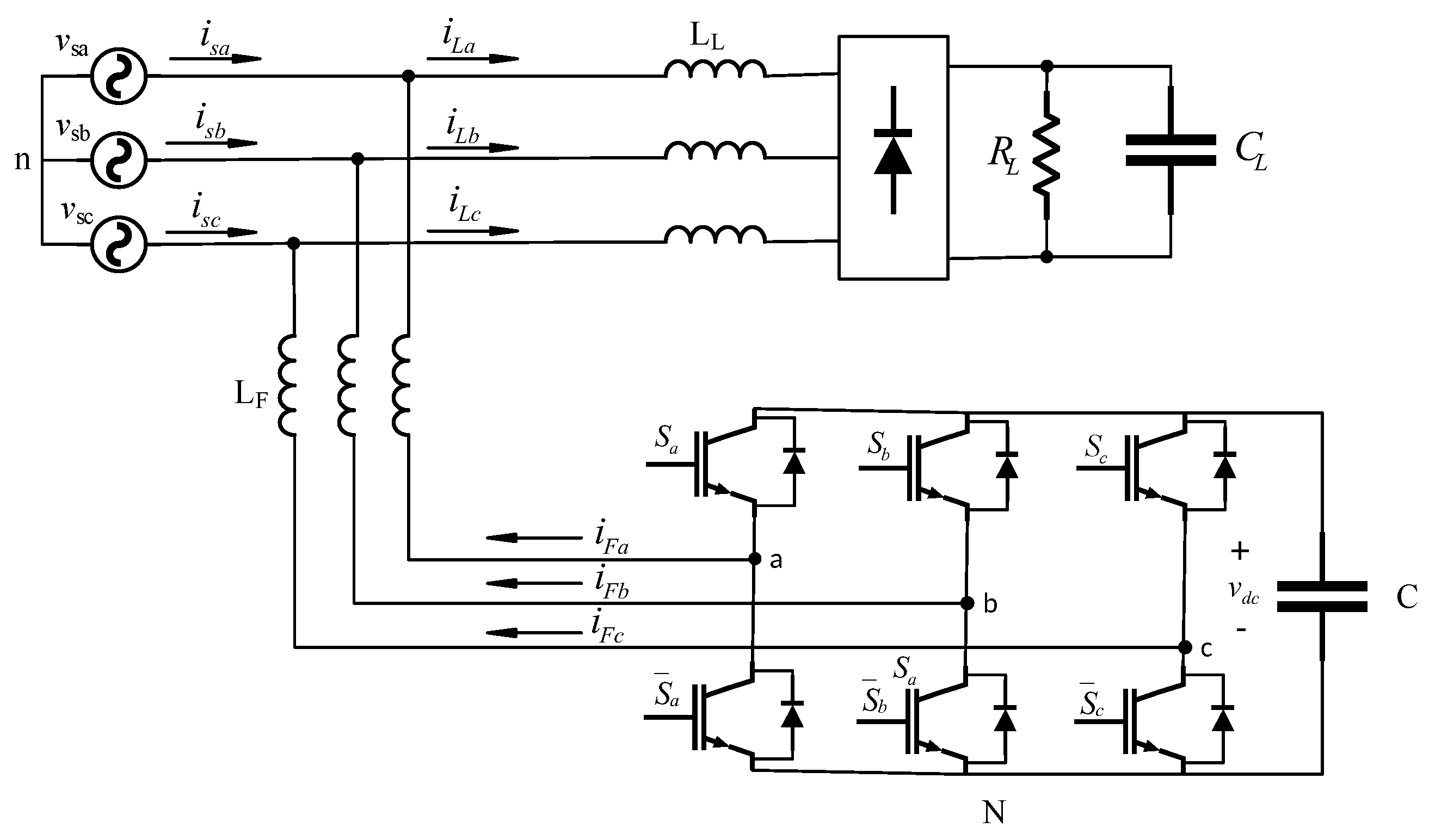
The three-phase SAPF circuit is shown in
Figure 1. From this circuit, the following equations for each phase-leg can be defined as follows:
These equations can be rewritten in terms of a space vector equation:
where
.
Now, by taking into account that
, the aforementioned equation can be rewritten as follows:
where
and
are the switching states such that
.
Equation (
5) can be separated into the real and imaginary parts corresponding to the
and
components:
Discrete-Time Model
In the FS-MPC a discrete converter model is required in order to predict the current n samples ahead. Usually, the predicted current is calculated from the discrete differential equation. Unlike other papers of the same topic, this paper uses a KF to estimate the current and the PCC voltages of the SAPF. The implementation of the observer will be presented in the next subsection.
The proposed continuous model in
frame is obtained by combining Equations (
9) and (
10) with:
From (
9)–(
12) the following space sate model is obtained:
where
and
the grid angular frequency. The space state model can be discretized according to the first order approximation. Then, by considering a sampling period
we obtain:
where
and
and
are the process and the measurement noise vectors respectively, which defines the following noise and process covariance matrices:
3. Proposed Control System
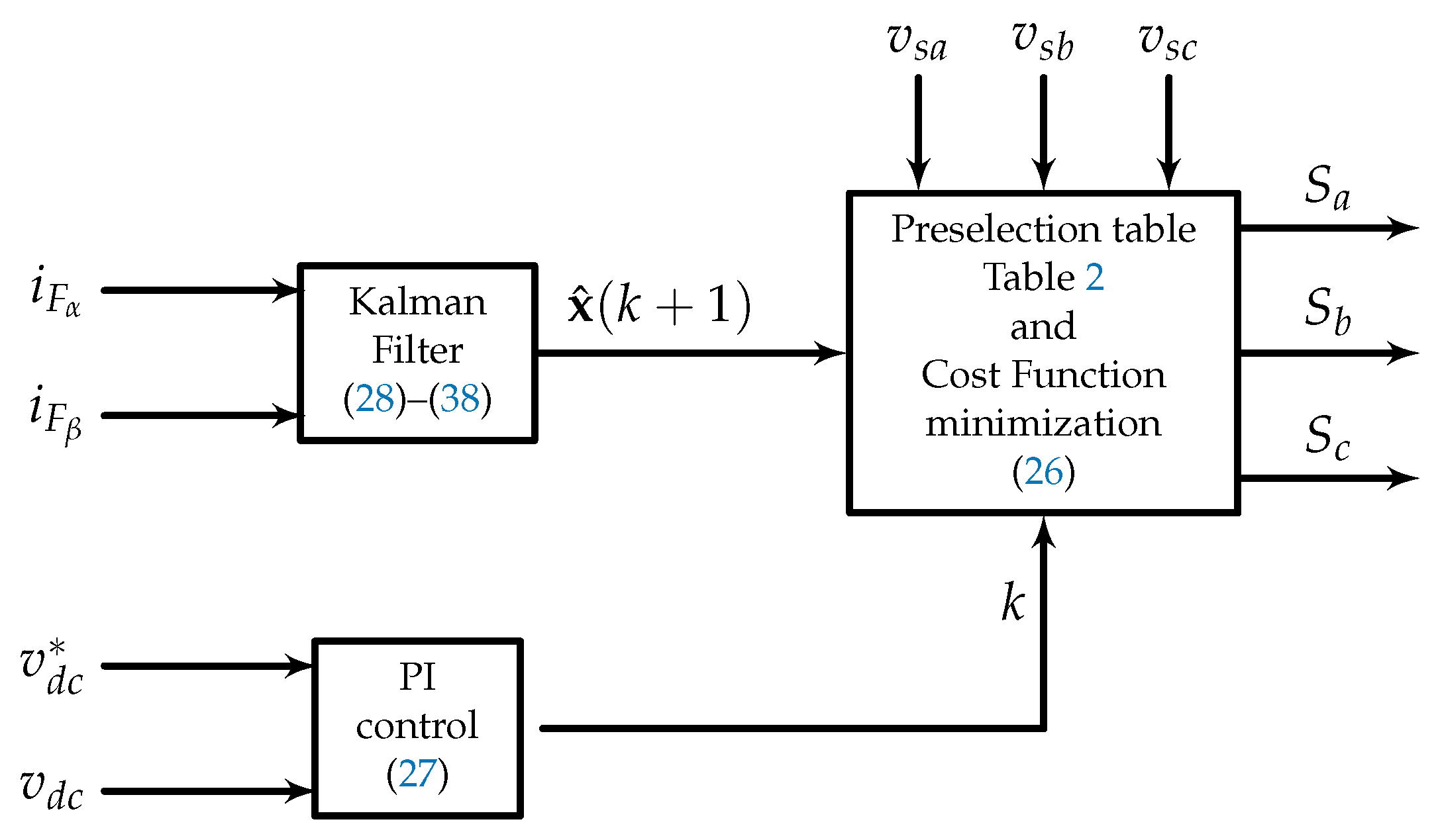
The proposed control diagram is depicted in
Figure 2. A KF is used in order to estimate the states variables one sample in advance. The PI controller regulates the filter output voltage and also is used to obtain the value of the gain
k in order to calculate the reference currents. This gain and the state estimation are the inputs of a cost function. First, a previous vector pre-selection task is done and only four possible vectors will be considered. Then, for each one of these selected vectors, the error between the predicted grid current and its reference is computed in order to find the optimum one which minimizes the error. Once the optimum is obtained, the switching state associated to this vector is applied to the converter. In the next sections, this control algorithm is explained in detail.
4. FCS-MPC with Reduced States
4.1. Principle
The FCS-MPC is based on the predictive control technique where the system under control has a finite number of switching states. The goal is to obtain the optimum switching state from a cost function which minimizes the error between a predicted state variable and its reference. According to the power converter shown in
Figure 1, eight switching states should be considered. However, if the grid voltage is dived in six 60° regions, the number of possible switching states can be reduced to four, as it will be shown latter. As a consequence, the computational load of the control algorithm will be clearly reduced.
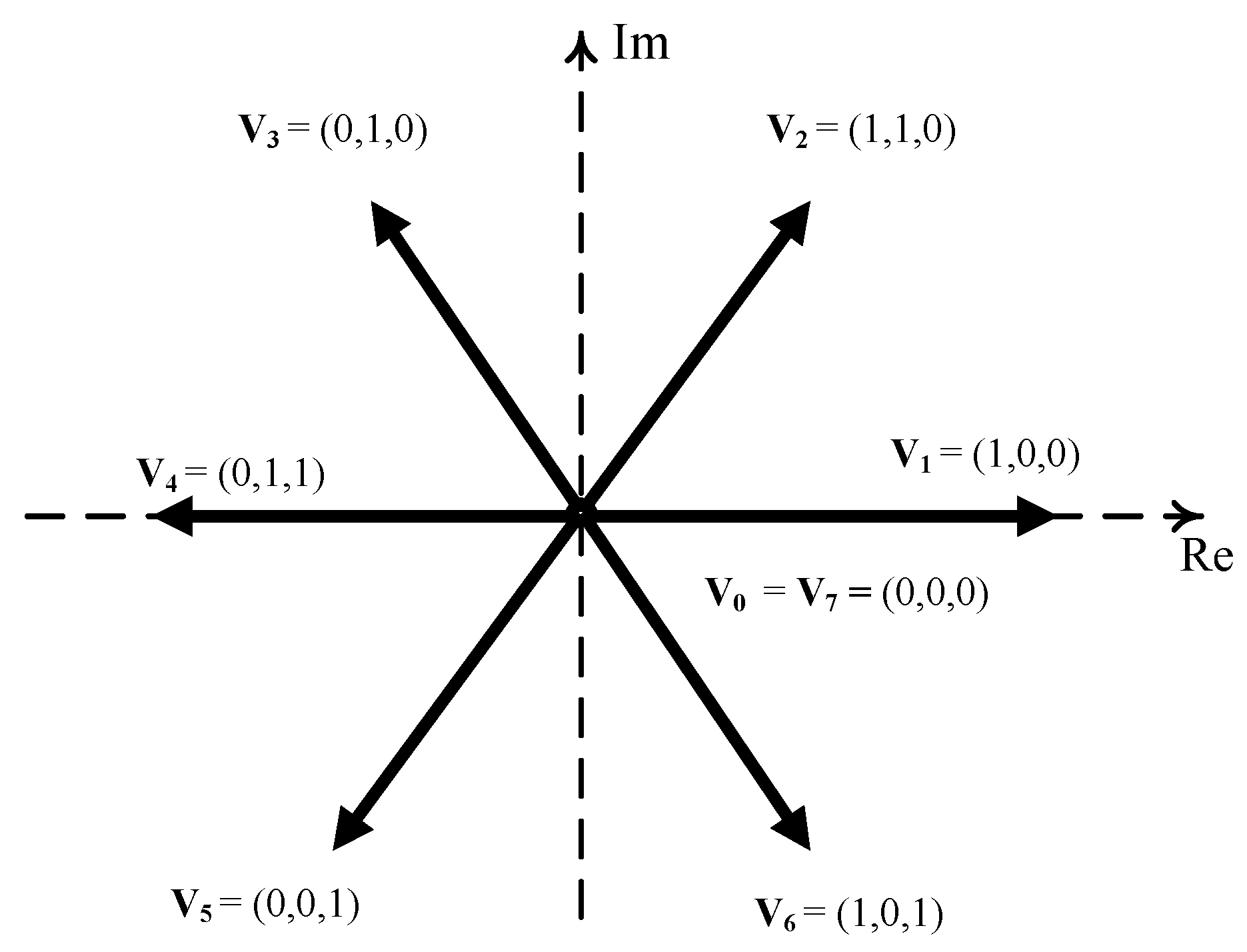
4.2. Vector Selection Based on Vector Operation
Equation (8) shows that different control switching states result in eight different voltage vectors which are represented in
Figure 3. Accordingly, the voltage vector
can take eight different values for each switching state. In
Table 1, the SAPF voltage,
, is represented according to each switching state:
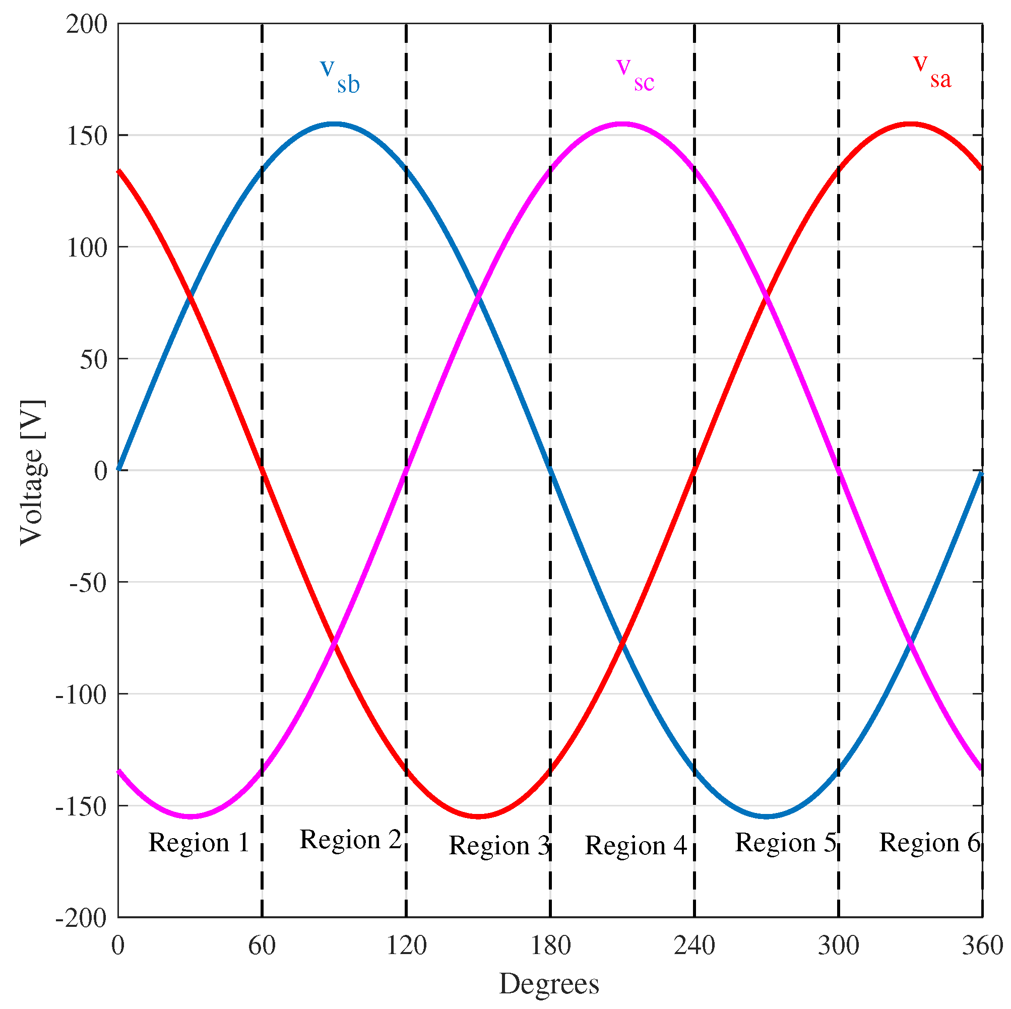
According to the sign of the grid voltages, the grid period can be divided into six 60° regions.
Figure 4 shows one period of the three-phase grid voltages. As it can be seen, only two grid voltages have the same sign (positive or negative) in each region, and their corresponding phase-legs are selected as high frequency legs. Note that, the remaining phase-leg is maintained to a constant dc voltage,
or
which is determined according to the vector operation technique [
14], as follows:
when the sign of two grid voltages is positive, the top switch of the remaining phase-leg is set in OFF state while the bottom switch is in ON state during this interval.
when the sign of two grid voltages is negative, the top switch of the remaining phase-leg is set in ON state while the bottom switch is in OFF state during this interval.
With this solution the eight possible vectors are reduced to four, in each 60° region (
Figure 4). Therefore, only four vectors will be considered in the computation of the optimum voltage vector to be applied to the power converter.
Looking at
Figure 4 and according to
Table 1, the algorithm can be summarized as shown
Table 2 where 1 is related to
and 0 to
.
Where symbols + and − are related to the positive or negative signs of the grid voltage and the symbol × is related to the high frequency phase-legs. As it can be seen, the combination of the FS-MPC with the vector operation techniques leads to a reduction to a half of the number of voltage vectors to be considered in each region, and as a consequence, a reduction of the computational time.
4.3. Cost Function Minimization Procedure
As mentioned before, a cost function is used to select the adequate converter voltage vector which satisfies the minimum error between the grid current and its reference. Then, the switching state which provides the optimal voltage vector is applied to control the SAPF. Let us define the following cost function in
frame:
where
and
are the reference currents obtained from the estimated PCC voltages, and
and
are the estimated grid currents, being
and
the load currents, and
k a gain obtained from a Proportional-Integral (PI) controller, and expressed as:
with
and
the proportional and integral gains respectively.
4.4. Kalman Filter
In order to reduce the noise of the close loop system, a Kalman filter is considered in this paper as an alternative to other prediction methods [
8]. A prediction of the filter currents and the PCC voltages are obtained in order to be used in a cost function presented in the next section. A modification in the KF algorithm is adopted in order to compensate the delay between the control process and the sampling instant [
15]. The main idea consist on substituting the measurement
for
in Equation (21). For a better understanding, a brief explanation of the KF algorithm is presented below. However, in [
15], a block diagram of the modified KF algorithm is presented in order to understand clearly the its implementation.
The KF can be considered as an optimum state observer in presence of noise. Then, the main idea consist of obtaining the best estimation of the states but eliminating the effect of the noise. For this purpose the Kalman gain is computed according to the noise covariance matrix in order to minimize the mean square error between the measured values of the states and the predicted ones. The Kalman gain expression is as follows:
where
is the a priori error covariance and
is given by (
24). The implementation of the traditional KF algorithm has two parts: (1) measurement update and (2) time update. The recursive steps are defined as follows:
First, in the measurement update step, the measurements and the error covariance matrix is computed as follows:
where
is the identity matrix and
is the Kalman gain defined in (
28).
In the next step, the time update step, a new prediction of the states and the error covariance matrix is done, that is:
Note that in this procedure, the algorithm is estimating the states at time
k, since the measurement,
, is obtained also at time
k. Therefore, in order to overcome the system delay between the sampling time and the control precoces, a modification in the traditional KF is adopted. As mentioned before, the modified KF algorithm substitutes the value of
for
in order to estimate one step in advance, thus compensating any delay in the system. Then, the modified algorithm is obtained by substituting (
29) in (
31) but using
instead of
obtaining:
Since the value of the sample
is unknown, this term must be removed from the observer equation. For this purpose an auxiliary variable
is used:
then
or at the sampling instant
:
Now, using (
33) in (
36) the term
is cancelled in the expression of
:
and replacing (
34) in (
37) we obtain the final recursive expression for
:
Equation (
38) is computed recursively in order to obtain
. Then,
is used in (
34) in order to obtain the estimated states one sample in advance. The final step is to update this estimation using Equation (29).
5. Experimental Results
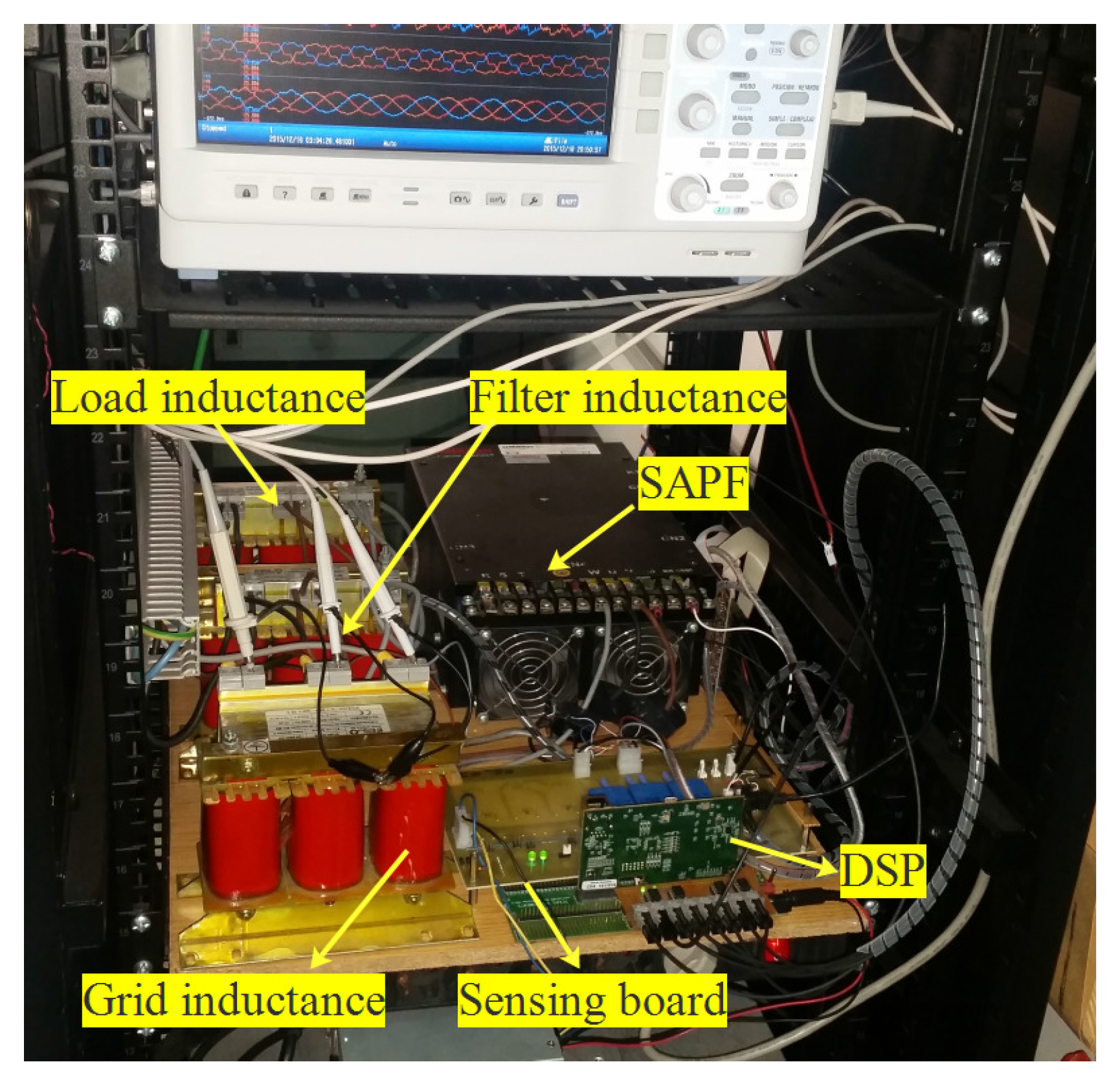
The prototype of the SAPF is shown if
Figure 5. The prototype has been built using a 4.5-kVA SEMICRON full-bridge as the power converter and a TMS320F28M36 floating point DSP as the control platform. The grid is generated using a PACIFIC 360-AMX source. The system parameters are listed in
Table 3.
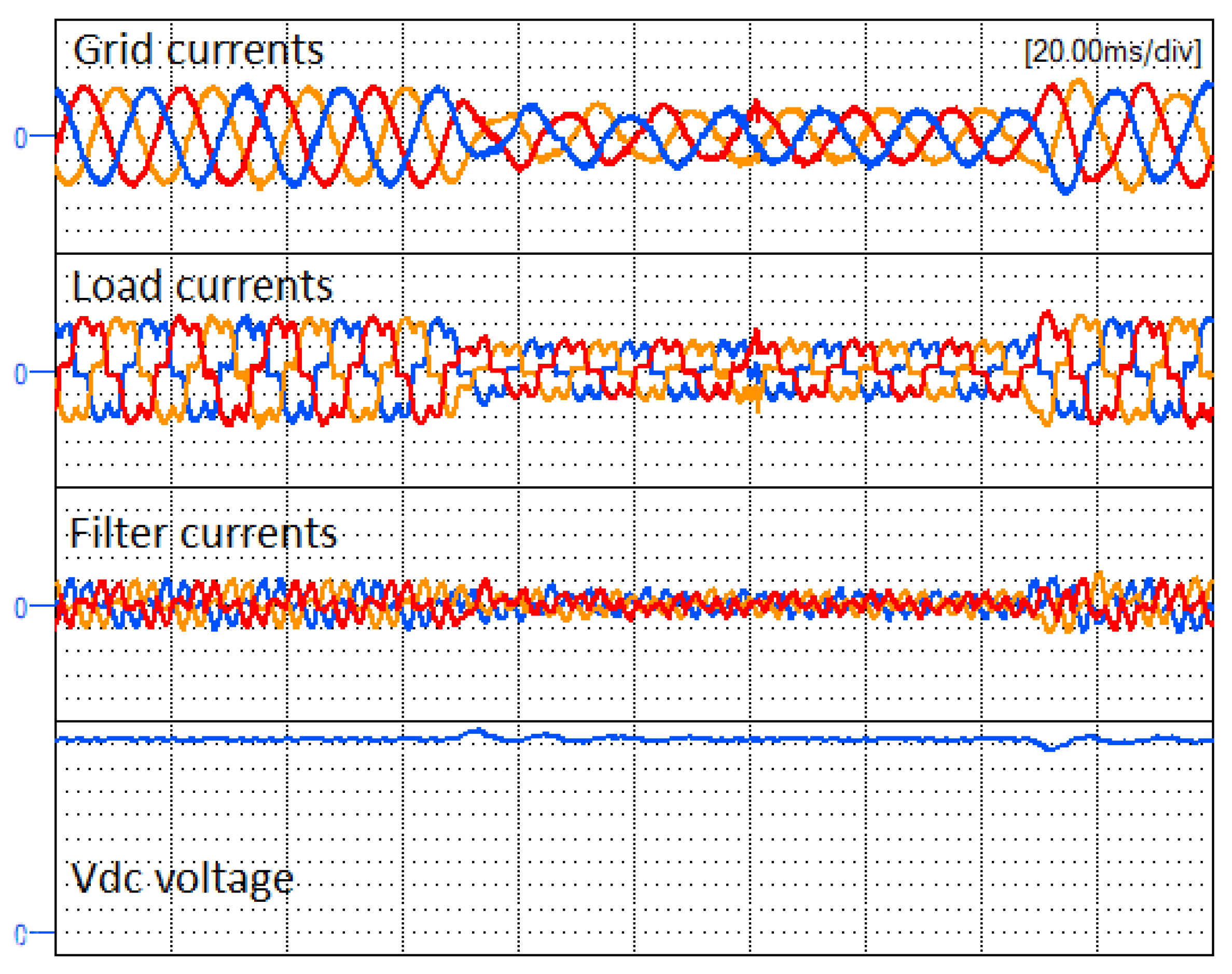
5.1. Response of the SAPF to Load Variations
Figure 6 show the main waveforms of the SAPF in case of a sudden load step change. The changes in the load are from full-load to half-load and half-load to full-load. The figure shows from top to bottom the grid currents, the non-linear load currents, the filter currents and the output voltage. It can be observed from the figure that the distortion caused by the load is perfectly compensated by the filter, providing sinusoidal grid currents. In order to validate the performances of the SAPF, the harmonic spectrum of the grid current for phase-leg
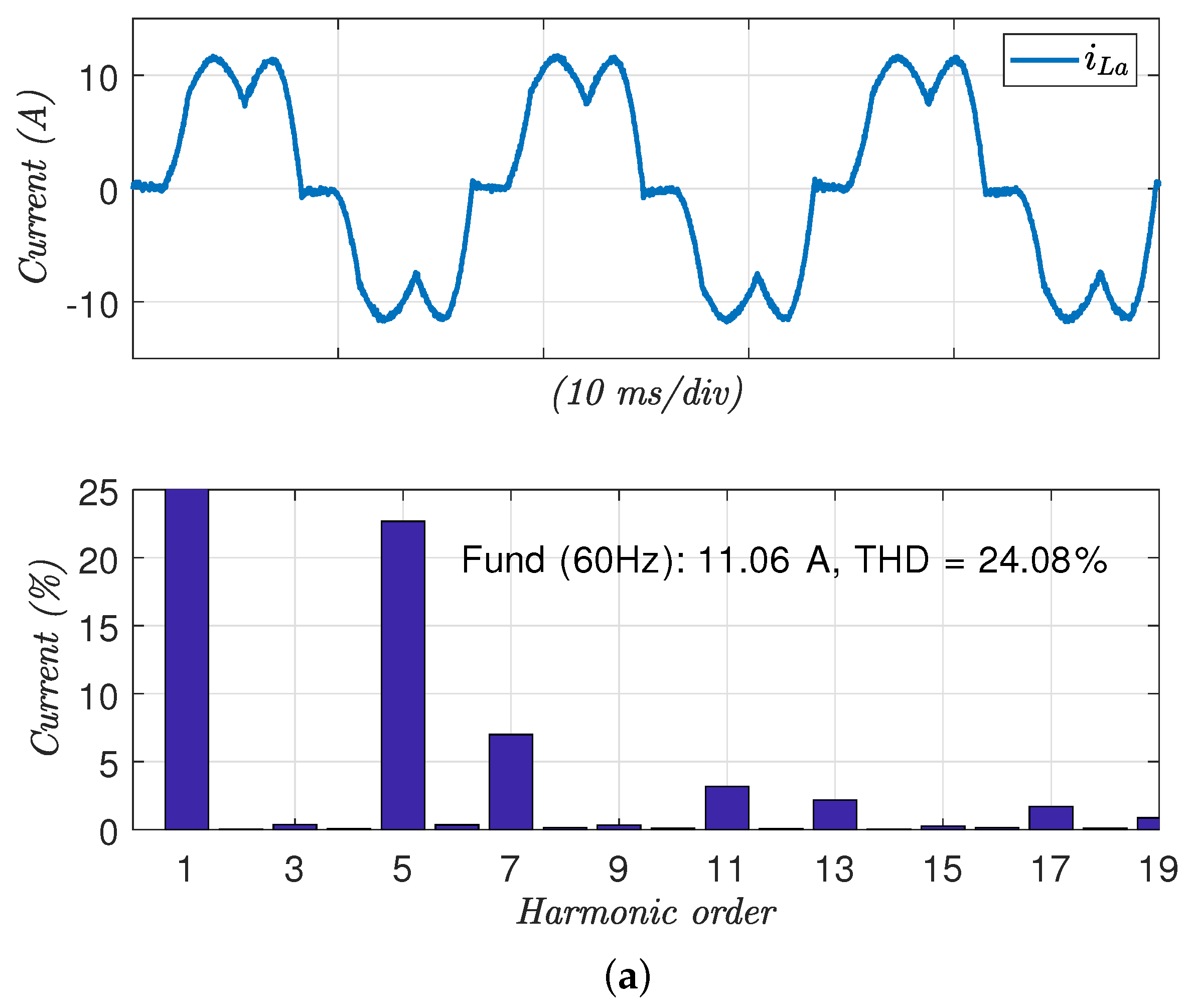
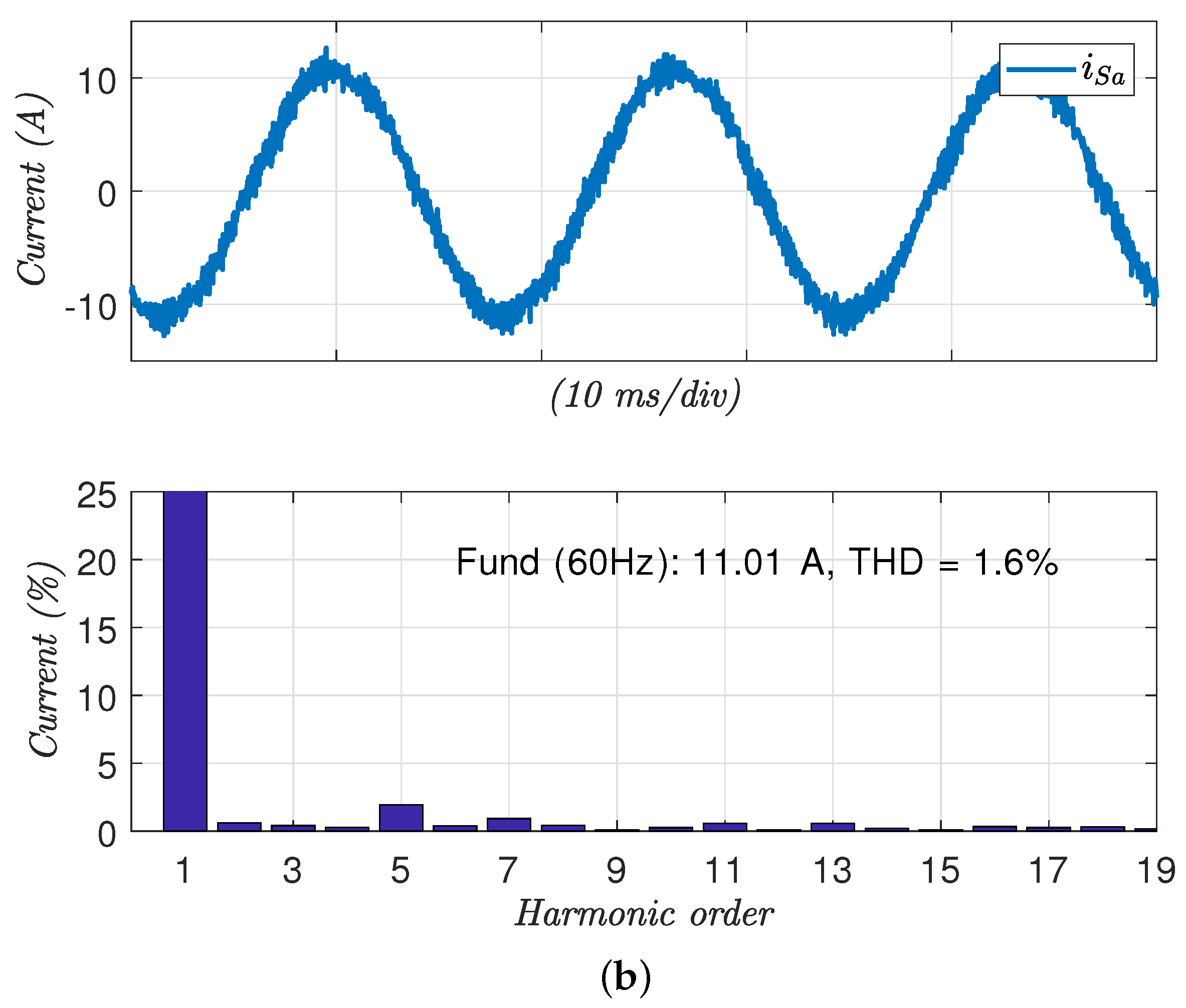
a is shown.
Figure 7 compares the THD after and before the compensation.
Figure 7a shows the spectrum before compensation, which THD is 24.08% while
Figure 7b shows the spectrum of the grid currents after the filter compensation which THD is 2.04%. An important reduction of the THD is achieved showing the good performances of the control algorithm.
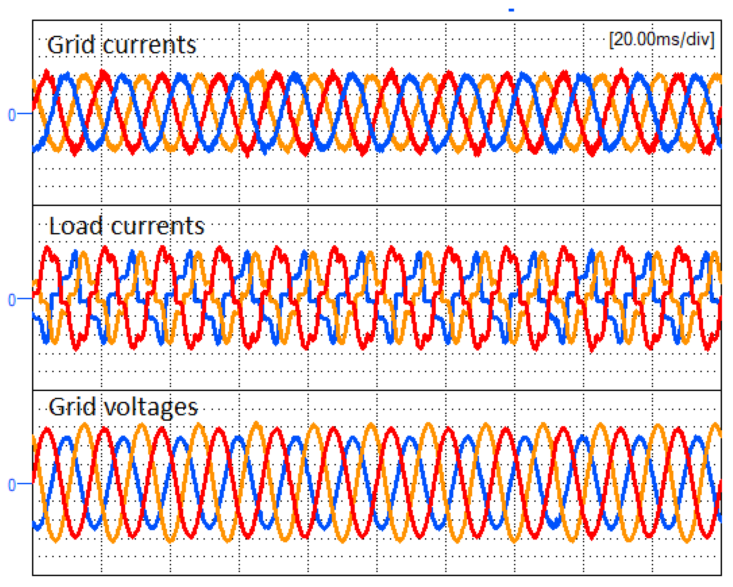
5.2. SAPF Performances under a Distorted Grid
In
Figure 8 the performances of the proposed controller in the case of a distorted grid is presented. This figure illustrates from top to bottom: the grid currents, the load currents and the distorted grid voltages which THD is around 14%. Even in case of grid harmonics, the grid currents are practically sinusoidal thanks to the good estimation of the grid voltages which allows to generate the reference current only with the fundamental component of the grid voltage. This is an interesting property of the proposed method since any synchronization system as for instance a phase-locked loop (PLL) is not needed. Note that by augmenting the number of harmonics in system matrix (15), an estimation of the
n-harmonics can be performed.
5.3. SAPF Performances under Grid Voltage Sags
In
Figure 9 the VSI performances when a grid voltage sag is done. The sag is characterized by a positive and negative sequences of
= 0.8 p.u. and
= 0.4 p.u. respectively. The phase angle between sequences is around
. The reference currents can be obtained using only the positive sequence of the PCC voltages according to
. In order to obtain the positive sequences, the expressions presented in [
16] can be used. Since the grid current tracks only the positive sequence of the PCC voltage, the current amplitude is maintained constant during the voltage sag.
6. Comparative Analysis
In this section a comparison between the proposed control algorithm with the conventional FCS-MPC is performed.
Table 4, gives a comparison based on the execution time
of the controller, computational load and memory usage in bytes is performed. The computational load can be computed according to:
As shown
Table 4, the execution time for the complete control algorithm is around 15
s (this is the case of considering only four vectors). In case of considering eight vectors (traditional FCS-MPC), the execution time is increased up to 23
s, as expected. The KF is designed according to [
3], where only the Kalman gain for one phase leg is computed, and considered equal for the remaining phases. This is because the system noise is similar in the three-phase legs. With this assumption, the time employed by the KF in the traditional FCS-MPC (eight vectors) is around 18
s, while in case of the proposed method (four vectors) is reduced to 10
s. Note that, this reduction is not exactly proportional to the number of voltage vectors. The remaining time to complete the values presented in
Table 4, is due to the remaining parts of the control algorithm.
In order to obtain the execution time, one timer of the DSP is used to measure the time of the controller task. In the conventional FCS-MPC the prediction of the grid voltages and currents is done eight times, one time for each vector, while with the proposed control algorithm this computation is reduced to only four vectors in each sampling period. As it can be seen, the total time employed by the algorithm is noticeably smaller. Thanks to this, the sampling frequency can be increased from 40 kHz in the conventional FCS-MPC up to 60 kHz for the proposed control algorithm. In the same way as in SMC happens, the relation between sampling frequency and switching frequency should be around ten. Then, the increment of the switching frequency yields to an improvement of the THD of the grid currents. One advantage of the proposed controller is that the algorithm can be implemented in the traditional signal processor without the necessity of using faster processor such as Field Programmable Gate Arrays (FPGAs).
7. Conclusions
In this paper, a combination between the FCS-MPC and the vector operation technique has been presented. The main advantage of combining both techniques is that for each region the number of possible voltage vectors to be considered is reduced to a half, thus reducing the computational load of the control algorithm. Besides, in each region, only two phase-legs are switching at high frequency while the remaining phase-leg is maintained to a constant voltage value during this interval. Accordingly, a reduction of the switching losses is obtained. As a difference with other MPC proposals, the proposed control algorithm make use of a KF in order to predict one sample ahead the three-phase currents and PCC voltages. Selected experimental results have been reported to prove the validity of the proposed controller.
Acknowledgments
This work has been supported by the European Union Project ELAC2014/ESE0034 and its linked to Spanish National Project PCIN-2015-001 and also supported by the Ministry of Economy and Competitiveness of Spain under project ENE2015-64087-C2-1-R.
Author Contributions
All authors have contributed to this work. R.G. is the main author of this manuscript and has conceived the theoretical analysis, modeling, simulation together with L.G.d.V., M.C., J.M. and A.C. helped to obtain the experiments and to make some corrections in the manuscript.
Conflicts of Interest
The authors declare no conflict of interest.
References
- Nguyen, T.N.; Luo, A.; Shuai, Z.; Chau, M.T.; Li, M.; Zhou, L. Generalised design method for improving control quality of hybrid active power filter with injection circuit. IET Power Electron. 2014, 7, 1204–1215. [Google Scholar] [CrossRef]
- Beres, R.N.; Wang, X.; Liserre, M.; Blaabjerg, F.; Bak, C.L. A Review of Passive Power Filters for Three-Phase Grid-Connected Voltage-Source Converters. IEEE J. Emerg. Sel. Top. Power Electron. 2016, 4, 54–69. [Google Scholar] [CrossRef]
- Guzman, R.; de Vicuna, L.G.; Morales, J.; Castilla, M.; Miret, J. Model-Based Control for a Three-Phase Shunt Active Power Filter. IEEE Trans. Ind. Electron. 2016, 63, 3998–4007. [Google Scholar] [CrossRef] [Green Version]
- Musa, S.; Amran, M.; Hizam, H.; Izzri, N.; Hoon, Y.; Ammirrul, M. Modified Synchronous Reference Frame Based Shunt Active Power Filter with Fuzzy Logic Control Pulse Width Modulation Inverter. Energies 2017, 10, 758. [Google Scholar] [CrossRef]
- Kanjiya, P.; Khadkikar, V.; Zeineldin, H.H. Optimal Control of Shunt Active Power Filter to Meet IEEE Std. 519 Current Harmonic Constraints Under Nonideal Supply Condition. IEEE Trans. Ind. Electron. 2015, 62, 724–734. [Google Scholar] [CrossRef]
- Tarisciotti, L.; Formentini, A.; Gaeta, A.; Degano, M.; Zanchetta, P.; Rabbeni, R.; Pucci, M. Model Predictive Control for Shunt Active Filters with Fixed Switching Frequency. IEEE Trans. Ind. Appl. 2017, 53, 296–304. [Google Scholar] [CrossRef]
- Nguyen, T.H.; Kim, K.H. Finite Control Set–Model Predictive Control with Modulation to Mitigate Harmonic Component in Output Current for a Grid-Connected Inverter under Distorted Grid Conditions. Energies 2017, 10, 907. [Google Scholar] [CrossRef]
- Hu, J.; Cheng, K.W.E. Predictive Control of Power Electronics Converters in Renewable Energy Systems. Energies 2017, 10, 515. [Google Scholar] [CrossRef]
- Kouro, S.; Cortes, P.; Vargas, R.; Ammann, U.; Rodriguez, J. Model Predictive Control A Simple and Powerful Method to Control Power Converters. IEEE Trans. Ind. Electron. 2009, 56, 1826–1838. [Google Scholar] [CrossRef]
- Trabelsi, M.; Bayhan, S.; Ghazi, K.A.; Abu-Rub, H.; Ben-Brahim, L. Finite-Control-Set Model Predictive Control for Grid-Connected Packed-U-Cells Multilevel Inverter. IEEE Trans. Ind. Electron. 2016, 63, 7286–7295. [Google Scholar] [CrossRef]
- Kou, P.; Liang, D.; Li, J.; Gao, L.; Ze, Q. Finite-Control-Set Model Predictive Control for DFIG Wind Turbines. IEEE Trans. Autom. Sci. Eng. 2017. [Google Scholar] [CrossRef]
- Qi, C.; Chen, X.; Tu, P.; Wang, P. Cell-by-Cell-Based Finite-Control-Set Model Predictive Control for a Single-Phase Cascaded H-Bridge Rectifier. IEEE Trans. Power Electron. 2017. [Google Scholar] [CrossRef]
- Hassine, I.M.B.; Naouar, M.W.; Mrabet-Bellaaj, N. Model Predictive-Sliding Mode Control for Three-Phase Grid-Connected Converters. IEEE Trans. Ind. Electron. 2017, 64, 1341–1349. [Google Scholar] [CrossRef]
- Morales, J.; de Vicuña, L.G.; Guzman, R.; Castilla, M.; Miret, J.; Torres-Martínez, J. Sliding mode control for three-phase unity power factor rectifier with vector operation. In Proceedings of the IECON 2015—41st Annual Conference of the IEEE Industrial Electronics Society, Yokohama, Japan, 9–12 November 2015. [Google Scholar]
- Ahmed, K.; Massoud, A.; Finney, S.; Williams, B. Sensorless Current Control of Three-Phase Inverter-Based Distributed Generation. IEEE Trans. Power Deliv. 2009, 24, 919–929. [Google Scholar] [CrossRef]
- Guzman, R.; de Vicuna, L.G.; Morales, J.; Castilla, M.; Miret, J. Model-based Active Damping Control for Three-Phase Voltage Source Inverters with LCL Filter. IEEE Trans. Power Electron. 2017, 32, 5637–5650. [Google Scholar] [CrossRef] [Green Version]
© 2017 by the authors. Licensee MDPI, Basel, Switzerland. This article is an open access article distributed under the terms and conditions of the Creative Commons Attribution (CC BY) license (http://creativecommons.org/licenses/by/4.0/).

 ,
, 


