Combining a Genetic Algorithm and Support Vector Machine to Study the Factors Influencing CO2 Emissions in Beijing with Scenario Analysis

Department of Economics and Management, North China Electric Power University, Baoding 071003, China
*
Author to whom correspondence should be addressed.
Energies 2017, 10(10), 1520; https://doi.org/10.3390/en10101520
Submission received: 21 August 2017
/
Revised: 15 September 2017
/
Accepted: 25 September 2017
/
Published: 2 October 2017
Abstract
:In recent years, Beijing has been facing serious environmental problems. As an important cause of environmental problems, a further study of the factors influencing CO2 emissions in Beijing has important significance for the social and economic development of Beijing. In this paper, Cointegration and Granger causality test were proposed to select influencing factors of CO2 emissions prediction in Beijing, the influencing factors with different leading lengths were checked as well, and the genetic algorithm (GA) was used to optimize the initial weight and threshold values of a support vector machine (SVM) and the new SVM optimized by GA (GA-SVM) was established to predict the CO2 emissions of Beijing from 2016–2020 with scenario analysis. Through the comparison of 36 kinds of development scenarios, we found that economic growth, resident population growth and energy intensity enhancement were the major growth factors of carbon emissions, of which the contributions exceed 0.5% in all kinds of development scenarios. Finally, this paper put forward some reasonable policy recommendations for the control of CO2 emissions.
1. Introduction
In 2014, the IPCC’s Fifth Assessment Report (AR5) showed that the cumulative CO2 emissions largely determined the global mean surface warming in the late 21st century and later, and even if carbon dioxide emissions were stopped, many aspects of climate change would continue for centuries. The report also pointed out that human activity was the main reason for climate change since the 1950s and unless the greenhouse gas emissions were controlled, global warming would reach a dangerous level in the future [1,2]. Global carbon project website statistics show that in 2015 the global total CO2 emissions reached 36.2 billion tons, of which China accounted for 28.77%, more than the sum of the United States and the European Union [3]. In recent years, China has taken active measures to combat climate change and China pledged that the CO2 emissions per unit of GDP would decrease by 60–65% in 2030 compared with 2005 at the Paris International Climate Conference in 2015 [4]. Furthermore, China’s government issued the “13th Five-Year Plan for the Control of Greenhouse Gas Emissions”, of which the main objective was to reduce CO2 emissions per unit of GDP by 18% in 2020 based on 2015 and the total amount of CO2 emissions had been effectively controlled [5]. Beijing, as one of the most developed cities in China and a core city in global competition, can further improve its comprehensive strength by reducing its CO2 emissions and carbon intensity and developing a low-carbon economy. Thus, there is a great need to introduce a scientific forecast model based on profound analysis of the influencing factors to predict CO2 emissions and then take practical and effective actions to achieve the goal of transforming Beijing into a low-carbon city.
Various approaches have been used to forecast CO2 emissions in recent years. Ahmed [6] introduced cointegration incorporated with an Auto Regressive Distributed Lag bounds testing approach to investigate the relationship between CO2 emissions and the main influencing factors in Pakistan with time series data from 1971 to 2008 based on the assumption of an environmental Kuznets curve. Similarly, Chinese scholars (e.g., Shao [7], Tong [8], Yin et al. [9] and Lin et al. [10]) also carried out research on the environmental Kuznets curve for China’s carbon emissions and analyzed the main factors that affected carbon emissions based on data from certain provinces or cities. Holden [11] constructed a benchmarking methodology for UK greenhouse gas emissions estimation in road freight transport, integrating weight utilization, capacity utilization, driving distance and associated greenhouse gas emissions with a data envelopment analysis (DEA) method and then tested it in a group of simulated fleets. Sheinbaum et al. [12] studied the energy and CO2 emissions trends of Mexico’s iron and steel industry from 1970–2006 using international comparisons and log mean divisia index. This paper held the opinion that energy efficiency improvement and share compression of fuel had a significant influence on CO2 emissions reduction. Based on a least squares support vector machine, Sun et al. [13] analyzed CO2 emission change trends of residential consumption and three major industries as well as proposed cointegration and Granger causality test to select influence factors of three major industries and residential consumption CO2 emissions. Through the above studies, the main factors that influence carbon emissions include economic progress, population indices, energy intensity, industrial structure and technical level, etc.
Because of the objective and quantifiable advantages of qualitative analysis, the studies of carbon emissions are always based on models with mathematical functions. However, the situation in the real world is complicated and a single model cannot cover all possibilities. Therefore, combined with scenario analysis, a model can predict CO2 emissions in different scenarios effectively and provide better assistance for energy forecasting, optimizing and planning [14]. Azam et al. [15] adopted a long-range energy alternatives planning (LEAP) model to estimate the energy consumption and CO2 emissions of road transportation in Malaysia from 2012 to 2040 under a business-as-usual scenario and three other alternative fuel policy scenarios: biodiesel vehicles (BIO), natural gas vehicles (NGV) and hybrid electric vehicles (HEV). The finding implied that the road transportation energy consumption and carbon emissions reduction of Malaysia were most effective under a natural gas vehicle (NGV) scenario. Kumar [16] employed a LEAP model to construct different energy scenarios and estimated CO2 emissions with the least cost method and then discussed the application of renewable energy in India’s future power supply system. The finding showed that under the Accelerated Renewable Energy Technology (ARET) scenario, renewable energy could probably account for 23% of the electricity generation and the carbon emissions could decrease 74% by 2050. Combined with scenario analysis, Liu [17] set three scenarios in the different applications of economic development mode and different traffic development mode using the LEAP model to forecast the main carbon emissions of the Jiangxi transportation industry in 2010–2030. The results showed that increasing the scope of using the new energy and renewable energy would help achieve the sustainable development of energy and the environment.
The abovementioned studies mostly selected a country, province or industry as the research object, which could effectively reflect the general characteristics of CO2 emissions in the macro field. However, the specific carbon emissions characteristics of a city could not be reflected. Feng et al. [18] analyzed the development trend of energy demand, energy structure and CO2 emissions of Beijing under three different scenarios of business-as-usual, basic-policy and low-carbon from 2007–2030. Their findings showed that the building and transport sectors were identified as promising fields for achieving low-carbon growth in Beijing over the next decades. By constructing a LEAP-Shanghai model, Chang [19] designed three comprehensive scenarios, i.e., the baseline scenario, the emissions reduction scenario and the enhanced emissions reduction scenario. This study proved that the key to long-term energy-savings and carbon emissions reduction was to exercise a reasonable control over the growth rate of economic development. In order to find suitable scenarios for the Beijing-Tianjin-Hebei rejoin, Wen [20] chose some potential driving factors of carbon emissions to build extended stochastic impacts by regression on stochastic impacts by regression on a population, affluence and technology (STIRPAT) model. The results showed that improvement of technological level, adjustment of industry and energy consumption structures were critical factors for the control of carbon emissions. Li [21] introduced the back propagation (BP) neural network optimized by improved particle swarm optimization algorithm (IPSO) to calculate the carbon emissions and carbon intensity reduction potential under various scenarios for 2016 and 2020 in Beijing. The results indicated that energy structure adjustment, industrial structure adjustment and technical progress could drive the decline in carbon intensity. However, the LEAP model relies mainly on the judgment of experts, which has strong subjectivity. Multiple collinearity problems can easily arise between different influencing factors in the STIRPAT model and the BP neural network algorithm is likely to lead to low model accuracy, premature or overfitting problems [22]. Therefore, looking for a more appropriate method in forecasting of carbon emissions is imperative.
Support vector machine (SVM) shows excellent performance in solving small samples, nonlinear and high dimensional estimation problems [23], suggesting it has a great potential in forecasting carbon emissions. However, the standard SVM approach also has some limitations, and the parameter setting of the SVM is crucial to improve its performance. In this paper, we introduce a novel carbon emissions prediction approach combining a genetic algorithm and support vector machine (GA-SVM) to enhance the prediction precision, in which GA is employed to optimize the parameters of SVM. Meanwhile, in order to solve the overfitting problem caused by outliers in the data, slack variable is introduced to support vector machine (SVM) and in this way the outliers can exist as a common point, so that neither the support vector machine nor hyperplane can be affected by it. In particular, cointegration and Granger causality test are proposed to select the influencing factors of CO2 emissions prediction in Beijing as well as check the influence factors with different leading lengths [13]. Then, the CO2 emissions prediction can be obtained under different scenarios using the selected factors, and we can find the major influencing factors of CO2 emissions among the comparisons of 36 kinds of scenarios.
The rest of this paper is organized as follows: in Section 2, a genetic algorithm (GA) is used to optimize the initial weight and threshold values of a support vector machine (SVM) and the new SVM optimized by GA (GA-SVM) is proposed, then we use cointegration and Granger causality test to select the influencing factors of CO2 emissions prediction and present the analysis of the data. Section 3 sets the scenario parameters and presents a brief description of different scenarios; Section 4 forecasts the CO2 emissions in Beijing from 2016–2020 and compares the prediction results under different scenarios; According to the comparison results, some recommendations for improvement are put forward in Section 5.
2. Method and Data
In this work, a GA-SVM model has been employed to forecast carbon emissions, because SVM has a superior forecasting performance and GA can be used to select suitable parameters for SVM. In accordance with the purpose of this paper, the following procedures were formulated: optimizing the parameters of SVM model with GA and then training GA-SVM model; calculating the CO2 emissions with the conversion formula in Beijing from 1990 to 2015; selecting the factors influencing CO2 emissions with cointegration and Granger causality test. Before these procedures were carried out, we briefly introduce the genetic algorithm and support vector machine and described how the genetic algorithm optimized support vector machine in detail. In addition, the raw data of CO2 emissions in Beijing from 1990 to 2015 is obtained through the conversion of fossil fuel combustion depending on the China Energy Statistical Yearbook and Beijing Statistical Yearbook.
2.1. Genetic Algorithms
Genetic algorithm (GA) is a global optimization search algorithm, proposed by the University of Michigan’s John Holland [24]. It is based on natural selection and genetic theory to simulate biological selection, crossover and mutation and finally get the optimal solution. Because genetic algorithms are robust, random, global, and suitable for parallel processing, they are always used to solve various complex optimization problems. In the optimization process, GA generates multiple starting points randomly in the solution space and starts the search at the same time. The fitness function is used to guide the search direction. Therefore, group search strategy and genetic operators are two main characteristics of genetic algorithm. Genetic algorithms belong to category of evolutionary algorithms, which use techniques inspired by natural evolution, such as inheritance, mutation, selection and crossover, to solve optimization problems. However, the performance of GA will be greatly affected by the determinations of genetic operators so that the selection of parameters needs further study to overcome this weakness. The basic steps of the genetic algorithm are as follows:
- (1)
- Encoding the parameters and obtaining the population chromosomes;
- (2)
- Calculating the fitness value of each individual in the population based on the fitness function;
- (3)
- Obtaining the new population after selection, crossover, and mutation operations;
- (4)
- Repeating step 2 and step 3 until the default conditions are met.
2.2. Support Vector Machine
Support Vector Machine (SVM) originated from the Statistical Learning Theory proposed by Vapnik [25] in 1995. It constructs the optimal separating hyperplane on the principle of structural risk minimization seeking to minimize the classification error of unknown samples, which makes it have a good generalization performance in the case of small sample. The basic concept of SVM is to map nonlinearly original data into a higher dimensional feature space to solve the linear problem. Thus, considering the set of data , where is the input vector, is the corresponding output value, i = 1, 2,…, n. the SVM regression function takes the form:
where is the non-linear mapping function from the input space x, which denotes the high dimensional feature space. w is the weight vector and b is the bias term. w and b are estimated by minimizing the regularized risk function:
where 1/2 is the regularization term, C is the punishment parameter, which represents the ability of prediction for regression and is considered to specify the trade-off between the empirical risk and the model flatness. is the -insensitive loss function, which is defined as the following form:
In Equation (3), if the error of forecasting vale is equal or greater than , the loss equals , otherwise the loss equals zero.
To estimate w and b, Equation (2) is transformed into Equation (4) by introducing two positive slack variables and :
Minimize:
subject to:
where two slack variables and measure the error of the up and down sides, respectively.
The above formulation leads to maximization optimization problem [26], which is solved employing the following Lagrangian form:
Maximize:
subject to:
where , is Lagrangian multipliers, − corresponding data points are support vector.
An optimal weight vector of the regression hyperplane is obtained by calculating and :
Hence, the regression function is:
in Equation (7), known as the kernel function, where the value of kernel function equals the inner product of two vector and in the feature space and , that is K( = , where i, j = 1, 2,, m.
In SVM, the popular kernel functions are:
- Sigmoid function: =.
- Polynomial basis function: =.
- Radial basis function (RBF): = exp ().
Compared with two other kernel functions, fewer free parameters need to be determined using the radial basis function, thus, optimizing parameters will become easy. Moreover, SVMs constructed by radial basis function perform much better than polynomial basis function and sigmoid function ones. Thus, RBF is employed in SVM in this paper and the selection of C, and plays an important role in the forecasting performance of the SVM [27].
2.3. GA-SVM Model
As described previously, the forecasting performance of SVM is highly dependent on its parameters. In the proposed work, genetic algorithm (GA) is used to optimize the initial weight and threshold values of SVM and the new SVM optimized by GA can get a better training effect and improve the prediction accuracy. Figure 1 illustrates the proposed GA-SVM approach.
The detailed description is as follows:
- (1)
- Encoding and giving the initial species: in this study, the three parameters, C, and are encoded to generate chromosomes in a binary format. Thus, according to the calculation precision required, an initial population of chromosomes which represent the values of three parameters can be generated randomly.
- (2)
- Calculating the fitness function: a cross validation method is used in calculating the fitness function to prevent over-fitting or under-fitting phenomenon in GA-SVM model [28]. In M-fold cross validation, the training set is divided into M equal subsets. One of the subsets is taken as testing set in turn and (M-1) subsets are taken as training set in the SVM regression model, then the above procedure is repeated so that each subset is validated once [29]. We used five-fold cross validation in this paper. In addition, mean absolute percentage error (MAPE) is selected as the fitness function, which is as follows:where m represents the number of training samples; and are the actual and predicted values respectively. The chromosome with a smaller value of MAPE has a better chance of surviving in the next generation.
- (3)
- Genetic algorithm operators—selection, crossover and mutation operations—are carried out to generate the progeny. The chromosomes with better fitness values are more likely to be selected into the next generation using means of the roulette wheel. Genes between two chromosomes are exchanged randomly to find better solutions with a crossover probability of 0.7. Mutation is performed to alter binary code form 0 to 1 with a probability of 0.7. The evolutionary process is repeated from step 2 to step 3 until stop conditions are satisfied.
This paper introduces the Libsvm3.22 toolboxes in Matlab R2013b and trains the SVM with radial basis function kernel. According to the setting of parameters in the training function in the Libsvm3.22 toolboxes, the three parameters to be optimized in SVM can be obtained i.e., “−c” represents C, “−g” represents , “−p” represents . Since this paper trains SVM with the radial basis function kernel in the Libsvm3.22 toolboxes which has only one parameter . Therefore, the parameter “-g” can be used to set its value.
To enhance the reliability of the training results, 22 samples are picked as training samples at random, which are selected from data during 1990–2015 and the remaining four samples are used as the test group. The running result shows that the average test error of our GA-SVM model is 1.62%, which demonstrates conformance to the requirements to forecast the future carbon emissions in Beijing. In this paper, we use s cross validation approach in the GA-SVM model and the cross validation results are further optimized by the GA algorithm so that the uncertainty is reduced [30]. In this way, the presence of uncertainty will not have much impact on the prediction accuracy of the GA-SVM model and the fitting result and prediction precision are satisfactory. In summary, the forecasting accuracy of GA-SVM model maintains a level around 98%, indicating that the uncertainty does not reduce predicative capability for the model.
Table 1 gives the initial parameters of genetic algorithms used in the proposed GA-SVM model. The values of these parameters based on numerous experiments can provide the smallest MAPE on the training set.
2.4. Data Source and Conversion
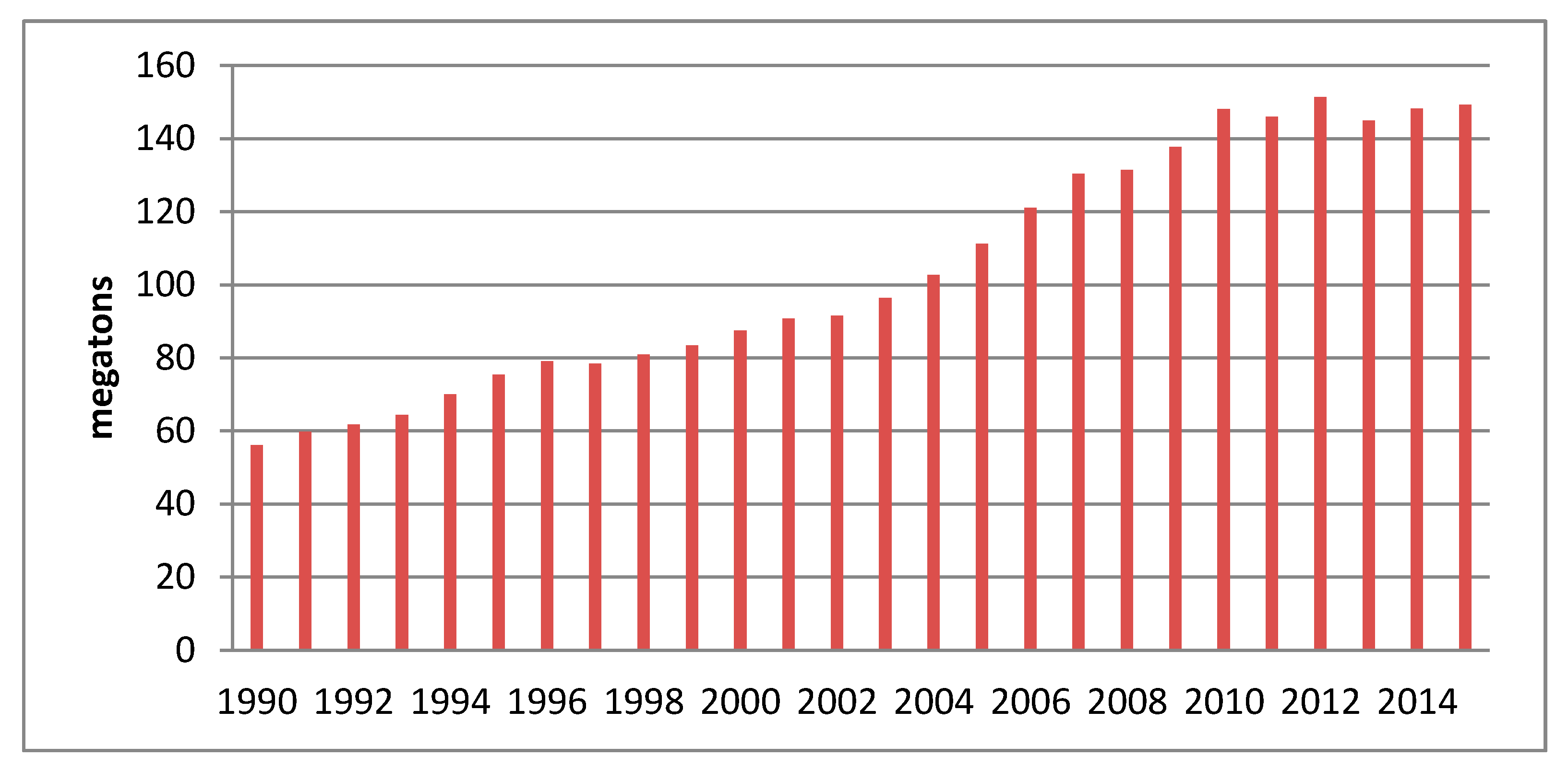
This paper chooses the energy consumption and other relevant data of Beijing from 1990 to 2015 and the CO2 emissions are calculated by the conversion formula. First of all, the annual energy consumption of different kinds of energy, including coal, coke, crude oil, gasoline, kerosene, diesel oil, fuel, natural gas and power are obtained from China Energy Statistical Yearbook and Beijing Statistical Yearbook. Secondly, the annual consumption data of the relevant fossil fuels are converted into standard coal according to the general calculation principle of comprehensive energy consumption. Table S1 shows the relevant conversion coefficients. Finally, according to the 2006 IPCC Guidelines for National Greenhouse Gas Inventories [31], the standard coal data can be converted into CO2 emissions by the conversion coefficients of different fossil fuels, which are shown in Table S2. In order to eliminate the impact of price factor, we calculate the value of per capita GDP and energy intensity based on the constant price of 1978, which is the base year. Thus, CO2 emissions from 1990–2015 in Beijing can be calculated as follows:
where C represents the total CO2 emissions, i is energy types, refers to CO2 emissions of energy i. represents the consumption of energy i, is the standard coal conversion coefficients of energy i, and refers to the CO2 emissions coefficients of energy i. The amount of CO2 emissions in Beijing from 1990 to 2015 according to Equation (9), is shown in Figure 2.
2.5. Cointegration and Granger Causality Test
In the macroeconomic econometric analysis, Engle and Granger [32] proposed the cointegration method that has become one of the most important tools to analyze the long-term equilibrium relationship between non-stationary economic variables. This paper employs Johansen test [33] for cointegratioin analysis between variables under the environment of EViews (Econometrics Views) 7.0.
Table 2 shows that there do exist cointegration relationships between CO2 emissions and per capita GDP, resident population, transportation possession quantity, technological level as well as energy intensity, whereas for economic structure and urbanization level, the Granger causality test may result in spurious regression for the variables have no cointegration relationship with CO2 emissions.
The cointegration test results show the existence of long-term stable correlation between CO2 emissions and the pre-selection factors but do not indicate the causality of them. Thus, the Granger causality test between these variables is required. Meanwhile, the Akaike information criterion (AIC) is used to select lags and the results are shown in Table 3.
As shown in Table 3, the suppositions that “Per capita GDP does not cause CO2 emissions”, “Resident population does not cause CO2 emissions”, “Transportation possession quantity does not cause CO2 emissions”, “Technological level does not cause CO2 emissions”, “Energy intensity does not cause CO2 emissions” are rejected on the significance level of 0.1, indicating that per capita GDP, resident population, transportation possession quantity, technological level and energy intensity will affect CO2 emissions under certain lag phases. Therefore, this paper chooses per capita GDP 2 years ahead (Lag2), resident population 3 years ahead (Lag3), transportation possession quantity 3 years ahead (Lag3), technological level 2 years ahead (Lag2) and energy intensity 2 years ahead (Lag2) as variables for SVM input when forecasting CO2 emissions.
3. Description of Scenarios
According to the results of cointegration test and Granger causality test, a total of 32 scenarios are set to forecast the CO2 emissions in Beijing from 2016–2020 based on different economic growth rates, resident population growth rates, transportation possession quantity growth rates, technical progress rates and energy intensity enhancement rates. The details are as follows.
3.1. Economic Growth Rates
Per capita GDP is an important indicator of China’s economic development, so economic growth rates are represented by per capita GDP growth rates in this paper. According to the 13th Five-Year Plan of Beijing’s National Economy and Social Development, the economic growth rates maintain medium-to-high during 2016 to 2020 and per capita income of urban and rural residents doubled by 2020 over 2010 [34]. However, with the fact that China’s economy steps into the “new normal” phase, a downward trend appears in economic growth of Beijing and it is expected to continue in the future [35]. In order to achieve the above targets, the per capita GDP growth rates cannot be less 6.5% in the 13th Five-Year Plan period [36]. Taking into account the domestic adjustment of economy structure and global economic downturn, economic growth rates of Beijing are set to medium and low categories form 2016 to 2020 (Table 4).
3.2. Resident Population Growth Rates
In view of the statistical yearbook of Beijing, the annual resident population growth rates in the 11th Five-Year Plan period and 12th Five-Year Plan period were 5% and 2.1%, respectively. In addition, population control was included in the government work report of Beijing for the first time in 2015, and a well-defined population control objective was proposed in the 13th Five-Year Plan for the removal of non-essential functions in Beijing [37]. Thus, the number of resident population in Beijing is probably expected to drop during the 13th Five-Year Plan. Therefore, the resident population growth rates in Beijing are set to medium and low categories form 2016 to 2020 (Table 5).
3.3. Transportation Possession Quantity Growth Rates
In the past two years, the transportation possession quantity growth had slowed down, but the amount was still on the rise [38], and the total demand for traffic will continue to grow with the economic and soc-ial development. At the same time, there is still a big gap in the traffic supply, and the contradiction between supply and demand of traffic is still the major contradiction for Beijing’s transportation in the future. It is expected that by 2020, the transportation possession quantity of Beijing will reach 6.3 million, which means that the annual growth rate will reach 3% [38]. However, the development of public transport and the promotion of green travel have become a major direction of the future transportation development in Beijing and this leads to the growth rate of transportation possession quantity slow down year by year [39]. Therefore, the transportation possession quantity growth rates in Beijing are set to medium and low categories from 2016 to 2020 (Table 6).
3.4. Technical Progress Rates
Due to the serious air pollution problems, Beijing requires a significant reduction in the proportion of coal used in primary energy consumption and an increase in natural gas consumption. By 2020, the annual consumption of natural gas in Beijing is planned to reach 20 billion cubic meters and the proportion of natural gas in energy consumption reaches 33% in the Development Plan of Gas Development in Beijing during the 13th Five-Year Plan period [40]. This means that Beijing will use natural gas as a major alternative energy after cutting coal consumption. According to the natural gas consumption data by province in National Bureau of Statistics of China, the natural gas consumption in Beijing was 14.688 billion cubic meters [41]. If the average annual growth rate reaches 4% over the next five years, the amount of natural gas consumption in Beijing will reach 20 billion cubic meters by 2020. However, the growth of natural gas consumption in Beijing maybe affected by the high price of natural gas. Also, because of the transformation of economic structure at present, there has been a slowdown in the growth of industrial used gas and gas for power generation in Beijing, which plays important roles in promoting the growth of natural gas consumption in Beijing [42]. Therefore, the technical progress rates of Beijing are set to medium and low categories from 2016 to 2020 (Table 7).
3.5. Energy Intensity Enhancement Rates
Energy consumption per ten thousand Yuan GDP of Beijing fell by 25.08% from 2011–2015, which is the only province in China that has completed the annual energy-saving target and is one year ahead of schedule to achieve the target that energy consumption per ten thousand Yuan GDP be reduced by 17% during the 12th Five-Year Plan period. In addition, the government announced that by 2020, energy consumption per ten thousand Yuan GDP of Beijing will decrease by 17% compared to 2015 [43]. Energy consumption divided by GDP is energy intensity so that we can obtain the energy intensity of Beijing in 2015 which was 1.928 tons of standard coal based on the constant price of 1978, and in order to achieve the target of 17%, the average annual enhancement rate of energy intensity will reaches −4% over the next five years. However, with the influence of global economic downturn, economic growth of Beijing is expected to slow down in the future. Therefore, the energy intensity enhancement rates of Beijing are set to medium and low categories from 2016 to 2020 (Table 8).
As shown in Table 9, in accordance with different energy intensity enhancement rates, this paper sets two main scenarios for Beijing form 2016 to 2020 i.e., the base development scenario and low carbon development scenario, each of which is composed of 16 kinds of series based on random combination of the five indexes.
4. Results and Discussion
The parameters of different development scenarios were used as predictive inputs of the GA-SVM model to predict carbon emissions in Beijing from 2016 to 2020, and then the growth rates of carbon emissions in 2020 based on 2016 in 32 kinds of scenarios were calculated. The prediction results in different scenarios were as follows.
4.1. Prediction Results of Carbon Emissions in the Base Development Scenario
The base development scenarios conclude 16 kinds of series, of which the energy intensity is set at low rate. The prediction values of carbon emissions of Beijing in 2016, 2018 and 2020 are shown in Figure 3.
Figure 3 shows the prediction results of carbon emissions of Beijing for the base development scenarios from 2016 to 2020, wherein carbon emissions in 2020 show an increase of about 2% to 5% compared with 2016 in all series. Through the comparison of the growth rate of carbon emissions in 2020 based on 2016, 16 kinds of scenarios can be divided into two categories: low growth rate (2−3%) of carbon emissions from scenario BD1 to BD8; high growth rate (3−5%) of carbon emissions from scenario BD9 to BD16, while carbon emissions in the former are higher than that in the latter. As we can know from Figure 3, carbon emissions will reach a peak in scenario BD3, in which the economic growth rate, resident population growth rate and transportation possession quantity growth rate are set at the medium level, and the energy intensity enhancement rate and technical progress rate are at the low level. In addition, carbon emissions will reach minimum in BD14, in which the economic growth rate, resident population growth rate, transportation possession quantity growth rate and energy intensity enhancement rate are at the low level, the technical progress rate is at the medium level.
It is obvious that the lower economic growth rate and transportation possession quantity growth rate are conducive to a decrease of CO2 emissions. In contrast, the higher technical progress rate contributes to reduce CO2 emissions. Through the comparison of BD1 and BD9 (BD2 and BD10, BD3 and BD11, BD4 and BD12, BD5 and BD13, BD6 and BD14, BD7 and BD15, BD8 and BD16), the contribution of economic growth rate on carbon emissions is 1.88%. Similarly, the contribution of resident population growth rate, transportation possession quantity growth rate and technical progress rate on carbon emissions are obtained, which are 0.57%, 0.28% and 0.18%. It means that if the economic growth rate increases by 1%, the carbon emissions will correspondingly increase by 1.88% in 2020 and if the resident population growth rate, transportation possession quantity growth rate and technical progress rate increase by 1%, the carbon emissions will increase by 0.57%, 0.28% and 0.18%, respectively, in 2020.
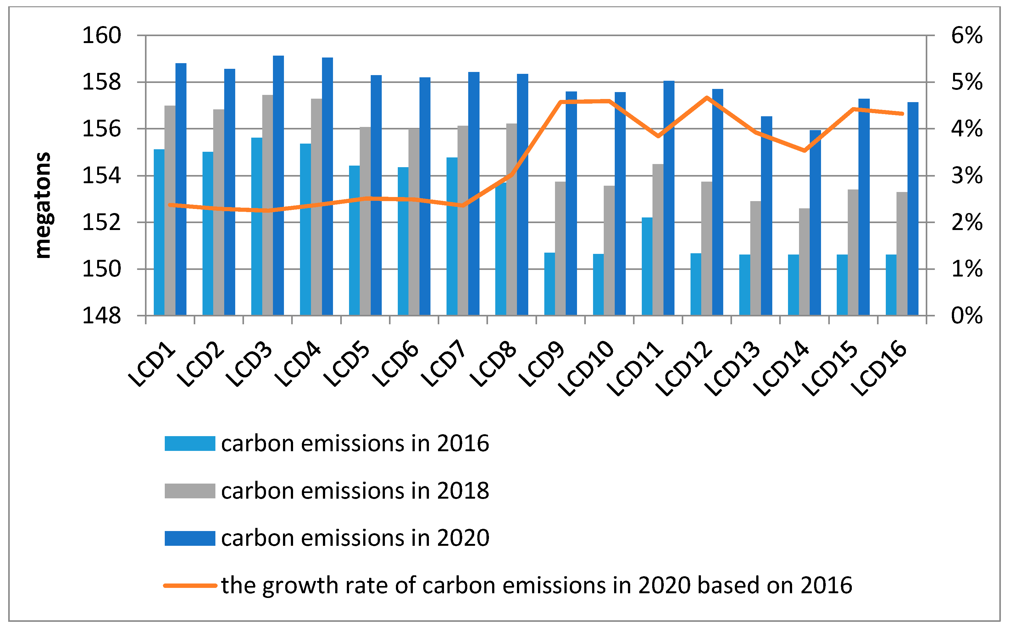
4.2. Prediction Results of Carbon Emissions in the Low Carbon Development Scenario
The low carbon development scenarios comprise 16 kinds of series, of which the energy intensity is set at medium rate. The prediction values of carbon emissions of Beijing in 2016, 2018 and 2020 are shown in Figure 4.
As shown in Figure 4, the prediction results for low carbon development scenarios indicate that carbon emissions from scenario LCD1 to LCD8 in 2020 are higher than ones from scenario LCD9 to LCD16, while the growth rate of carbon emissions in 2020 compared with 2016 in the former are higher than that in the latter, which within the range of 2−5%.In light of Figure 4 , carbon emissions will peak in scenario LCD3, in which the economic growth rate, resident population growth rate , transportation possession quantity growth rate and energy intensity enhancement rate are at the medium level, the technical progress rate is at the low level. Besides, carbon emissions will reach the lowest value in scenario14, in which the energy intensity enhancement rate and technical progress rate are at the medium level, the economic growth rate, resident population growth rate and transportation possession quantity growth rate are at the low level.
Through the comparison of LCD1 and LCD9 (LCD2 and LCD10, LCD3 and LCD11, LCD4 and LCD12, LCD5 and LCD13, LCD6 and LCD14, LCD7 and LCD15, LCD8 and LCD16), the contribution of economic growth rate on carbon emissions is 1.85%. Similarly, the contributions of resident population growth rate, transportation possession quantity growth rate and technical progress rate on carbon emissions are obtained, which are 0.54%, 0.36% and 0.21%. It means that if the economic growth rate increases by 1%, the carbon emissions will increase by 1.85% in 2020 correspondingly and if the resident population growth rate, transportation possession quantity growth rate and technical progress rate increase by 1%, the carbon emissions will increase by 0.54%, 0.36% and 0.21% respectively in 2020. Additionally, the contribution of energy intensity enhancement rate is 0.54% through the comparison of BD1 and LCD1 (BD2 and LCD2, BD3 and LCD3,…, BD15 and LCD15, BD16 and LCD16), which mean that if the energy intensity enhancement rate increases by 1%, the carbon emissions will increase by 0.54% in 2020.
4.3. Comparison between the Base Development Scenario and Low Carbon Development Scenario
Compared with the base development scenario, the prediction values of carbon emissions of Beijing for a low carbon development scenario in 2020 are lower under each corresponding scenario, such as BD1 and LCD1. The growth rates of carbon emissions in 2020 based on 2016 in the two main scenarios are similar, which start low and then ascend and fluctuate around 4% in the sequence of scenarios. The comparison of two main scenarios demonstrates that economic growth, resident population growth and energy intensity enhancement are the major growth factors of carbon emissions for Beijing during 2016 to 2020, of which the contributions exceed 0.5% in two main scenarios. However, transportation possession quantity growth and technical progress have no significant influence on the growth of carbon emissions, of which the contributions are less than 0.4% in two main scenarios. In conclusion, the comparison results prove that economic growth, resident population growth and energy intensity enhancement are the leading contributors to carbon emissions growth for Beijing. The comparison results for two main development scenarios are shown in Table 10.
5. Conclusions and Suggestions
After selecting influence factors with cointegration test and Granger causality test, this paper introduces GA-SVM model to forecast carbon emissions of Beijing from 2016 to 2020 under different scenarios. Through the comparison within the two main development scenarios, we can draw the conclusions that: (a) the average contribution of economic growth rate for carbon emissions is 1.865%, which is the biggest growth factor of carbon emissions; (b) the average contribution of resident population growth rate for carbon emissions is 0.555%, which is the second biggest growth factor of carbon emissions. Through comparing the base development scenario and low carbon development scenario, we can draw a conclusion that: (c) the average contribution of energy intensity enhancement rate for carbon emissions is 0.54%, which is also an important growth factor of carbon emissions. According to the analysis of CO2 emissions in two main scenarios, we find three key growth factors of CO2 emissions for Beijing, which are economic growth, resident population growth and energy intensity enhancement. Based on the conclusions mentioned above, policy recommendations are put forward to Beijing as follows:
- (a)
- Since CO2 emissions are closely related to the economic growth, it is essential to continue to transform the economic growth mode, adjust the industrial structure and optimize energy consumption for Beijing [44]. Considering that the per capita GDP of Beijing exceeded 110,000 yuan in 2016, which had reached the level of moderately developed countries, Beijing can achieve structural carbon emissions reduction through the industrial structure adjustment and optimal allocation of resources. This means that the dual objective of optimizing the economic structure and reducing carbon emissions can be achieved by optimizing the allocation of limited resources to the field that per unit output value for carbon emissions is lower. Although the proportion of tertiary industry has reached 77.9% in 2014, Beijing still needs to accelerate the development of producer services, such as finance, information, technology, commerce and circulation.
- (b)
- For the purpose of reducing CO2 emissions, limiting the increasing speed of resident population growth rate in Beijing is an important target and the resident population growth rate has dropped form 2.9% to 0.9% during 2011 to 2015. Furthermore, with a well-defined population control objective was proposed for the removal of non-essential functions in Beijing, even the negative growth of resident population will appear in the 13th Five-Year Plan period. The government should continue to implement such resident population control policies so that the CO2 emissions in Beijing will not grow further and reach peak as early as possible. Moreover, China has announced the establishment of the Xiong’an New Area (XNA) in Hebei Province, which is part of the measures to advance the coordinated development of the Beijing-Tianjin-Hebei region. It will help phase out excessive population, some economic management and service functions from Beijing, thereby reducing the carbon emissions.
- (c)
- Compared with foreign low carbon cities, such as Copenhagen, London and Stockholm, there still exists huge space to further reduce CO2 emissions by relying on reducing energy intensity. Beijing ought to reduce the energy intensity in key areas such as transportation and construction, as well as the services and tourism industry by administrative means and market mechanisms [45]. In addition, updating equipment, adopting advanced technology, strengthening energy management and conservation are imperative for Beijing to develop its low-carbon economy and build a global low-carbon city [46]. Besides, government should take full advantage of its Higher Educational Resources and provide financial subsidies to promote the development of renewable energy and increase the consumption ratio of clean energy, such as nuclear, wind and solar energy.
Supplementary Materials
The following are available online at www.mdpi.com/1996-1073/10/10/1520/s1, Table S1: Standard coal conversion coefficients of different kinds of energy, Table S2: CO2 emissions conversion coefficient for different kinds of energy.
Acknowledgments
This work has been supported by “Ministry of Education, Humanities and Social Science Fund, Nos. 15YJC630058”, “the Fundamental Research Funds for the Central Universities, Nos. 2017MS083”.
Author Contributions
Jinying Li designed this paper and provided overall guidance; Binghua Zhang wrote the paper; and Jianfeng Shi wrote and debugged the program. All authors read and agreed to the final article.
Conflicts of Interest
The authors declare no conflict of interest.
References
- Stocker, T.F.; Qin, D.; Plattner, G.K.; Tignor, M.; Allen, S.K.; Boschung, J.; Nauels, A.; Xia, Y.; Bex, V.; Midgley, P.M. Climate Change 2013: The physical science basis. contribution of working group I to the fifth assessment report of IPCC the intergovernmental panel on climate change. Comput. Geom. 2014, 18, 95–123. [Google Scholar]
- Zhang, X.H.; Gao, Y.; Qi, Y.; Fu, S. Implications of the findings from the working group I contribution to the IPCC fifth assessment report on the UNFCCC process. Adv. Clim. Chang. Res. 2014, 10, 14–19. [Google Scholar]
- Global Carbon Atlas. 2016. Available online: http://www.globalcarbonatlas.org/cn/CO2-emissions (accessed on 25 July 2017).
- Xinhua Net. “China Voice” at the Paris Climate Conference. 2015. Available online: http://news.xinhuanet.com/comments/2015–12/02/c_1117324305.htm (accessed on 25 July 2017).
- The State Council. The 13th Five-Year Plan for the Control of Greenhouse Gas Emissions. 2016. Available online: http://www.gov.cn/zhengce/content/2016–11/04/content_5128619.htm (accessed on 25 July 2017).
- Ahmed, K. Environmental kuznets curve and Pakistan: An empirical analysis. Procedia Econ. Financ. 2012, 1, 4–13. [Google Scholar] [CrossRef]
- Shao, F.; Qu, X.; Xi, Y. Carbon emissions and the environmental kuznets curve factors in Shaanxi province—An empirical analysis based on 1978–2008. J. Arid Land Resour. Environ. 2012, 26, 37–43. [Google Scholar]
- Lancet, T. The carbon emissions environmental kuznets curve and the impact factors—Empirical study on 103 cities in China. J. Basic Sci. Eng. 2012, 20, 119–125. [Google Scholar]
- Yin, J.; Zheng, M.; Chen, J. The effects of environmental regulation and technical progress on CO2 kuznets curve: An evidence from China. Energy Policy 2015, 77, 97–108. [Google Scholar] [CrossRef]
- Lin, B.Q.; Jiang, Z.J. Forecast of China’s environmental kuznets curve for CO2 emission and factors affecting China’s CO2 emission. Manag. World. 2009, 4, 27–36. [Google Scholar]
- Holden, R.; Xu, B.; Greening, P.; Piecyk, M.; Dadhicha, P. Towards a common measure of greenhouse gas related logistics activity using data envelopment analysis. Transp. Res. Part A 2016, 91, 105–119. [Google Scholar] [CrossRef]
- Sheinbaum, C.O.L.; Castillo, D. Using logarithmic mean Divisia index to analyze changes in energy use and carbon dioxide emissions in Mexico’s iron and steel industry. Energy Econ. 2010, 32, 1337–1344. [Google Scholar] [CrossRef]
- Sun, W.; Liu, M. Prediction and analysis of the three major industries and residential consumption CO2 emissions based on least squares support vector machine in China. J. Clean. Prod. 2016, 122, 144–153. [Google Scholar] [CrossRef]
- Li, B. Beijing Integrated Assessment Model for Low-Carbon Energy and 2030 Energy Strategy; Beijing University of Technology: Beijing, China, 2014. [Google Scholar]
- Azam, M.; Othman, J.; Begum, R.A.; Abdullah, S.M.S.; Nor, N.G.M. Energy consumption and emission projection for the road transport sector in Malaysia: An application of the LEAP model. Environ. Dev. Sustain. 2016, 18, 1027–1047. [Google Scholar]
- Kumar, S.; Madlener, R. CO2 emission reduction potential assessment using renewable energy in India. Energy 2016, 97, 273–282. [Google Scholar] [CrossRef]
- Liu, Y.Y.; Wang, Y.F.; Yang, J.Q.; Zhou, Y. Scenario analysis of carbon emissions in Jiangxi transportation industry based on LEAP model. Appl. Mech. Mater. 2011, 66–68, 637–642. [Google Scholar] [CrossRef]
- Feng, Y.Y.; Zhang, L.X. Scenario analysis of urban energy saving and carbon abatement policies: A case study of Beijing city, China. Procedia Environ. Sci. 2012, 13, 632–644. [Google Scholar] [CrossRef]
- Chang, Z.; Pan, K.X.; Fudan University. An analysis of Shanghai’s long-term energy consumption and carbon emission based on LEAP model. Contemp. Financ. Econ. 2014, 1079–1080, 502–505. [Google Scholar]
- Liu, Y.; Lei, W. The peak value of carbon emissions in the Beijing-Tianjin-Hebei region based on the STIRPAT model and scenario design. Pol. J. Environ. Stud. 2016, 25. [Google Scholar] [CrossRef]
- Li, J.; Shi, J.; Li, J. Exploring reduction potential of carbon intensity based on back propagation neural network and scenario analysis: A case of Beijing, China. Energies 2016, 9, 615. [Google Scholar] [CrossRef]
- Liu, H.-B.; Jiao, Y.-B. Application of genetic algorithm-support vector machine (GA-SVM) for damage identification of bridge. Int. J. Comput. Intell. Appl. 2011, 10, 383–397. [Google Scholar] [CrossRef]
- Shin, H.J.; Cho, S. Response modeling with support vector machines. Expert Syst. Appl. 2006, 30, 746–760. [Google Scholar] [CrossRef]
- Holland, J.H. Adaptation in Natural and Artificial Systems: An Introductory Analysis with Applications to Biology, Control, and Artificial Intelligence; University of Michigan Press: Ann Arbor, MI, USA, 1975. [Google Scholar]
- Vapnik, V.; Cortes, C. Support vector networks. Mach. Learn. 1995, 20, 273–297. [Google Scholar]
- Drucker, H.; Burges, C.J.C.; Kaufman, L.; Smola, A.J.; Vapnik, V. Support vector regression machines. Adv. Neural Inf. Process. Syst. 1996, 28, 779–784. [Google Scholar]
- Huang, C.L.; Wang, C.J. A GA-based feature selection and parameters optimizationfor support vector machines. Expert Syst. Appl. 2006, 31, 231–240. [Google Scholar] [CrossRef]
- Bishop, C.M. Pattern Recognition and Machine Learning (Information Science and Statistics); Springer-Verlag: New York, NY, USA, 2006. [Google Scholar]
- Sajan, K.S.; Kumar, V.; Tyagi, B. Genetic algorithm based support vector machine for on-line voltage stability monitoring. Int. J. Electr. Power Energy Syst. 2015, 73, 200–208. [Google Scholar] [CrossRef]
- Liu, S. Q.; Zhuang, Q.L.; He, Y.J.; Gu, L.H. Evaluating atmospheric CO2 effects on gross primary productivity and net ecosystem exchanges of terrestrial ecosystems in the conterminous United States using the AmeriFlux data and an artificial neural network approach. Agric. For. Meteorol. 2016, 220, 38–49. [Google Scholar] [CrossRef]
- Blobel, D.; Nils, M.-O.; Carmen, S.-A.; Penny, S. 2006 United Nations Framework Convention on Climate Change Handbook; Climate Change Secretariat (UNFCCC): Rio de Janeiro, Brazil, 2006. [Google Scholar]
- Granger, C.W.J. Investigating causal relations by econometric models and cross-spectral methods. Econometrica 1969, 37, 424–438. [Google Scholar] [CrossRef]
- Johansen, S. The statistical analysis of cointegration vectors. J. Econ. Dyn. Control 1988, 12, 231–254. [Google Scholar] [CrossRef]
- Beijing Municipal Committee of the CPC. The 13th Five-Year Plan of Beijing’s National Economy and Social Development. 2016. Available online: http://zhengwu.beijing.gov. cn/ghxx/sswgh/t1429796.htm (accessed on 25 July 2017).
- Xiao, H.W. The prediction of total energy consumption and structure change trend in Beijing city in 13th Five-Year period. China Energy 2015, 37, 38–42. [Google Scholar]
- Qianlong News. Target of Beijing in 13th Five-Year Plan: Average Annual Growth Rate of GDP Reaches 6.5%. 2016. Available online: http://beijing.qianlong.com/2016/0122/302433.shtml (accessed on 19 August 2017).
- China National Radio Network. Control the Population of Beijing Less than 23 Million During the 13th Five-Year Plan. 2016. Available online: http://news.cnr.cn/native/gd/20160122/t20160122_521203091.shtml (accessed on 19 August 2017).
- China National Radio Network. The Number of Motor Vehicles in Beijing Will Reach 6.3 Million in 2020. 2016. Available online: http://auto.cnr.cn/gdbkxw/20161026/t20161026_523221981.shtml (accessed on 19 August 2017).
- China News. The Total Mileage of Urban Railway in Beijing Will Reach 900 km During the 13th Five-Year Plan. 2016. Available online: http://www.chinanews.com/sh/2016/09–04/7993705.shtml (accessed on 19 August 2017).
- Beijing Municipal Commission of City Management. The Development Plan of Gas Development in Beijing during the 13th Five-Year Plan. 2017. Available online: http://www.bjmac.gov.cn/zwxx/zwtzgg/201703/t20170329_38911.html (accessed on 19 August 2017).
- National Bureau of Statistics of China. The Natural Gas Consumption Data by Province. 2017. Available online: http://data.stats.gov.cn/easyquery.htm?cn=E0103 (accessed on 19 August 2017).
- Zhao, R.; Wang, Y. Analysis of natural gas growth in Beijing. Chengshi Ranqi 2016, 6, 33–36. [Google Scholar]
- Beijing Municipal People’s Government. Beijing Has Exceeded Annual Energy Saving Target for Ten Consecutive Years. 2016. Available online: http://zhengwu.beijing.gov.cn/gzdt/bmdt/t1433446.htm (accessed on 19 August 2017).
- Fan, F.; Lei, Y. Factor analysis of energy-related carbon emissions: A case study of Beijing. J. Clean. Prod. 2015. [Google Scholar] [CrossRef]
- Wu, C. Low-Carbon Policy and action in the Chinese mainland: An overview of current development. Chin. Stud. 2014, 3, 157–164. [Google Scholar]
- Liu, W.; Qin, B. Low-carbon city initiatives in China: A review from the policy paradigm perspective. Cities 2016, 51, 131–138. [Google Scholar] [CrossRef]
Figure 1.
Flowchart for GA-SVM model.
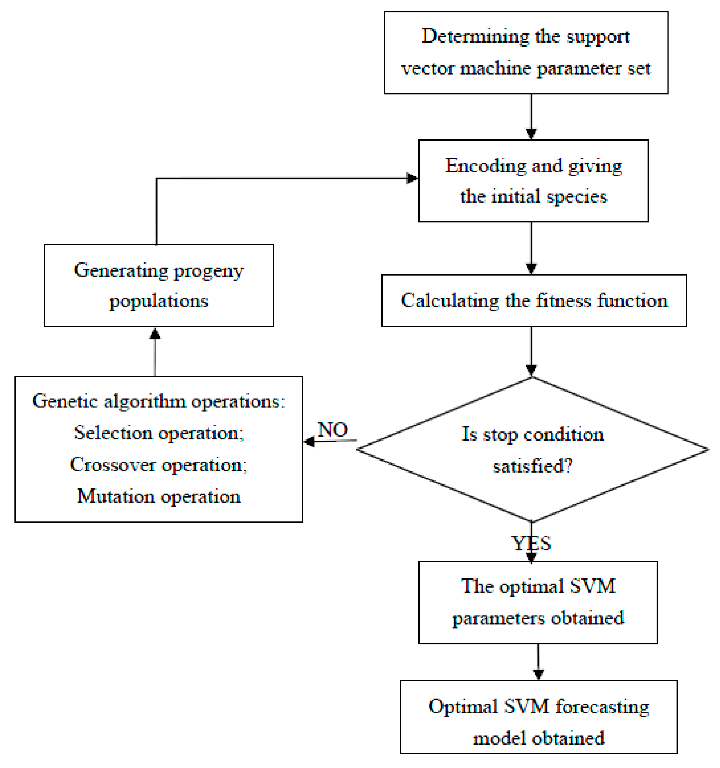
Figure 2.
CO2 emissions in Beijing from 1990 to 2015.

Figure 3.
The prediction values of carbon emissions of Beijing for the base development scenarios in 2016, 2018 and 2020.
Figure 3.
The prediction values of carbon emissions of Beijing for the base development scenarios in 2016, 2018 and 2020.
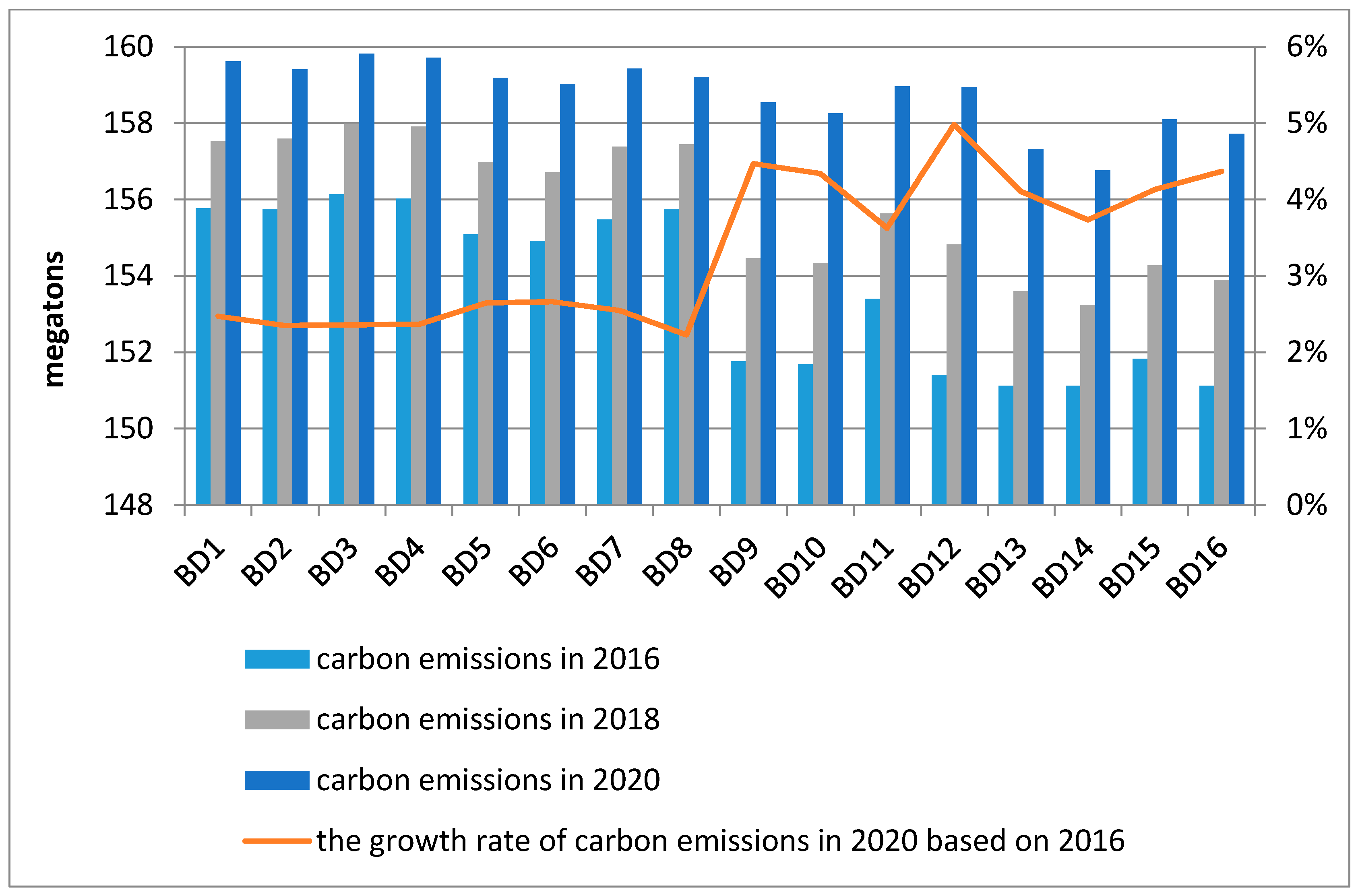
Figure 4.
The prediction values of carbon emissions of Beijing for low carbon development scenarios in 2016, 2018 and 2020.
Figure 4.
The prediction values of carbon emissions of Beijing for low carbon development scenarios in 2016, 2018 and 2020.


Table 1.
Parameters setting of genetic algorithms.
| Parameters | Settings |
|---|---|
| −c | 0–300 |
| −g | 0–300 |
| −p | 0.01 |
| Generations | 200 |
| Population size | 20 |
| Selection type | Standard roulette wheel |
| Crossover type | Simulated binary |
| Mutation type | Polynomial method |
| Crossover probability | 0.7 |
| Mutation probability | 0.7 |
Table 2.
Cointegration test results for CO2 emissions and pre-selection factors.
| Test Variables | Hypothesized No. of CE(s) | Eigenvalue | Trace Statistic | 0.05 Critical Value | Prob. 2 |
|---|---|---|---|---|---|
| CO2 emissions & Per capita GDP | None 1 | 0.518836 | 21.15532 | 20.26184 | 0.0376 |
| At most 1 | 0.139226 | 3.598173 | 9.164546 | 0.4752 | |
| CO2 emissions & Economic structure | None | 0.470941 | 18.02423 | 20.26184 | 0.6295 |
| At most 1 1 | 0.108058 | 2.744491 | 9.164546 | 0.0087 | |
| CO2 emissions & Resident population | None 1 | 0.596550 | 26.57363 | 20.26184 | 0.0059 |
| At most 1 | 0.180886 | 4.788759 | 9.164546 | 0.3074 | |
| CO2 emissions & Transportation possession quantity | None 1 | 0.490648 | 21.07830 | 20.26184 | 0.0385 |
| At most 1 | 0.184249 | 4.887497 | 9.164546 | 0.2960 | |
| CO2 emissions & Urbanization level | None | 0.365863 | 13.93259 | 18.39771 | 0.1568 |
| At most 1 1 | 0.117533 | 3.000809 | 3.841466 | 0.0266 | |
| CO2 emissions & Technological level | None 1 | 0.476593 | 20.81233 | 20.26184 | 0.0420 |
| At most 1 | 0.197307 | 5.274802 | 9.164546 | 0.2546 | |
| CO2 emissions & Energy intensity | None 1 | 0.667915 | 29.28885 | 15.49471 | 0.0002 |
| At most 1 | 0.111308 | 2.832115 | 3.841466 | 0.0924 |
1 denotes rejection of the hypothesis at the 0.05 level; 2 Mackinnon-Haug-Michelis (1999) p-values.
Table 3.
Granger causality test results for CO2 emissions and pre-selection factors.
| F-Statistic | Prob. | Lag | Conclusion | |
|---|---|---|---|---|
| Per capita GDP → CO2 emissions | 5.44933 | 0.0141 | 2 | Exist a Granger causality |
| Resident population → CO2 emissions | 3.14847 | 0.0272 | 3 | Exist a Granger causality |
| Transportation possession quantity → CO2 emissions | 2.53252 | 0.0162 | 3 | Exist a Granger causality |
| Technological level → CO2 emissions | 1.15594 | 0.0371 | 2 | Exist a Granger causality |
| Energy intensity → CO2 emissions | 2.78170 | 0.0000 | 2 | Exist a Granger causality |
Table 4.
Economic growth rates of Beijing form 2016 to 2020 (%).
| Year | Medium Growth Rate | Low Growth Rate |
|---|---|---|
| 2016–2020 | 6.7 | 5.5 |
Table 5.
Resident population growth rates of Beijing form 2016 to 2020 (%).
| Year | Medium Growth Rate | Low Growth Rate |
|---|---|---|
| 2016–2020 | 0.9 | −0.5 |
Table 6.
Transportation possession quantity growth of Beijing form 2016 to 2020 (%).
| Year | Medium Growth Rate | Low Growth Rate |
|---|---|---|
| 2016–2020 | 4 | 2.5 |
Table 7.
Technical progress rates of Beijing form 2016 to 2020 (%).
| Year | Medium Optimization Rate | Low Optimization Rate |
|---|---|---|
| 2016–2020 | 4 | 2.5 |
Table 8.
Energy intensity enhancement rates of Beijing form 2016 to 2020 (%).
| Year | Medium Optimization Rate | Low Optimization Rate |
|---|---|---|
| 2016–2020 | −4 | −3 |
Table 9.
Parameters setting of different development scenarios.
| Combination of Index Change Rate | |||||||||||
|---|---|---|---|---|---|---|---|---|---|---|---|
| Base Development Scenario | Low Carbon Development Scenario | ||||||||||
| SS | EG | PG | TG | EI | TP | SS | EG | PG | TG | EI | TP |
| BD1 | Medium | Medium | Low | Low | Low | LCD1 | Medium | Medium | Low | Medium | Low |
| BD2 | Medium | Medium | Low | Low | Medium | LCD2 | Medium | Medium | Low | Medium | Medium |
| BD3 | Medium | Medium | Medium | Low | Low | LCD3 | Medium | Medium | Medium | Medium | Low |
| BD4 | Medium | Medium | Medium | Low | Medium | LCD4 | Medium | Medium | Medium | Medium | Medium |
| BD5 | Medium | Low | Low | Low | Low | LCD5 | Medium | Low | Low | Medium | Low |
| BD6 | Medium | Low | Low | Low | Medium | LCD6 | Medium | Low | Low | Medium | Medium |
| BD7 | Medium | Low | Medium | Low | Low | LCD7 | Medium | Low | Medium | Medium | Low |
| BD8 | Medium | Low | Medium | Low | Medium | LCD8 | Medium | Low | Medium | Medium | Medium |
| BD9 | Low | Medium | Low | Low | Low | LCD9 | Low | Medium | Low | Medium | Low |
| BD10 | Low | Medium | Low | Low | Medium | LCD10 | Low | Medium | Low | Medium | Medium |
| BD11 | Low | Medium | Medium | Low | Low | LCD11 | Low | Medium | Medium | Medium | Low |
| BD12 | Low | Medium | Medium | Low | Medium | LCD12 | Low | Medium | Medium | Medium | Medium |
| BD13 | Low | Low | Low | Low | Low | LCD13 | Low | Low | Low | Medium | Low |
| BD14 | Low | Low | Low | Low | Medium | LCD14 | Low | Low | Low | Medium | Medium |
| BD15 | Low | Low | Medium | Low | Low | LCD15 | Low | Low | Medium | Medium | Low |
| BD16 | Low | Low | Medium | Low | Medium | LCD16 | Low | Low | Medium | Medium | Medium |
Note: SS represents scenario sequence, EG represents economic growth rate, PG represents resident population growth rate, TG represents transportation possession quantity growth rate, EI represents energy intensity enhancement rate, TP represents technical progress rate.
Table 10.
Comparison results for two main development scenarios.
| Base Development Scenario | Low Carbon Development Scenario | |
|---|---|---|
| Prediction values of carbon emissions | higher | lower |
| Movement trend of growth rates of carbon emissions in 2020 based on 2016 | Start between 2–3% and then fluctuate around 4% | Start between 2–3% and then fluctuate around 4% |
| the contribution of economic growth rate | 1.88% | 1.85% |
| the contribution of resident population growth rate | 0.57% | 0.54% |
| the contribution of energy intensity enhancement rate | 0.54% | 0.54% |
| the contribution of transportation possession quantity growth rate | 0.28% | 0.36% |
| the contribution of technical progress rate | 0.18% | 0.21% |
© 2017 by the authors. Licensee MDPI, Basel, Switzerland. This article is an open access article distributed under the terms and conditions of the Creative Commons Attribution (CC BY) license (http://creativecommons.org/licenses/by/4.0/).
Share and Cite
MDPI and ACS Style
Li, J.; Zhang, B.; Shi, J. Combining a Genetic Algorithm and Support Vector Machine to Study the Factors Influencing CO2 Emissions in Beijing with Scenario Analysis. Energies 2017, 10, 1520. https://doi.org/10.3390/en10101520
AMA Style
Li J, Zhang B, Shi J. Combining a Genetic Algorithm and Support Vector Machine to Study the Factors Influencing CO2 Emissions in Beijing with Scenario Analysis. Energies. 2017; 10(10):1520. https://doi.org/10.3390/en10101520
Chicago/Turabian StyleLi, Jinying, Binghua Zhang, and Jianfeng Shi. 2017. "Combining a Genetic Algorithm and Support Vector Machine to Study the Factors Influencing CO2 Emissions in Beijing with Scenario Analysis" Energies 10, no. 10: 1520. https://doi.org/10.3390/en10101520
Note that from the first issue of 2016, this journal uses article numbers instead of page numbers. See further details here.