Ensemble Prediction Model with Expert Selection for Electricity Price Forecasting

Abstract

Forecasting of electricity prices is important in deregulated electricity markets for all of the stakeholders: energy wholesalers, traders, retailers and consumers. Electricity price forecasting is an inherently difficult problem due to its special characteristic of dynamicity and non-stationarity. In this paper, we present a robust price forecasting mechanism that shows resilience towards the aggregate demand response effect and provides highly accurate forecasted electricity prices to the stakeholders in a dynamic environment. We employ an ensemble prediction model in which a group of different algorithms participates in forecasting 1-h ahead the price for each hour of a day. We propose two different strategies, namely, the Fixed Weight Method (FWM) and the Varying Weight Method (VWM), for selecting each hour’s expert algorithm from the set of participating algorithms. In addition, we utilize a carefully engineered set of features selected from a pool of features extracted from the past electricity price data, weather data and calendar data. The proposed ensemble model offers better results than the Autoregressive Integrated Moving Average (ARIMA) method, the Pattern Sequence-based Forecasting (PSF) method and our previous work using Artificial Neural Networks (ANN) alone on the datasets for New York, Australian and Spanish electricity markets.

1. Introduction

Deregulated electricity markets are becoming increasingly common, in line with the evolution of a range of smart grid initiatives. In a traditional fixed-priced electricity market, consumption of electricity follows a distinct and more-or-less regular peak demand curve. This peak demand forces the supplier to use resources to meet the peak demand, and those resources are redundant for rest of the time. To overcome this inefficiency, the concept of demand management is put forward as a part of the smart grid initiative [1]. A smart grid utilizes the information about the behaviors of supplier and consumers of electricity and tries to optimize the production and the distribution of electricity.

The smart grid enables two-way peer-to-peer communications between the energy supplier (e.g., a retailer) and the consumers. This distributed information flow, which takes an Internet-like form, will enable the supplier to price the energy based on the consumption feedback from the consumer. On the other hand, the consumers can also schedule their consumption behavior to achieve optimal utilization at the lowest possible cost. In addition, nowadays, a substantial portion of energy is generated from renewable resources, like wind and solar, which are naturally less predictable than the traditional resources, like fossil fuel. All of these factors create a dynamism in the electricity market, under which the main concern for the supplier is to manage a healthy ratio between demand and supply. The general idea of demand management is to design a pricing mechanism that decides the hourly prices that can persuade the consumers to change their usage patterns in order to lower the peak demand, with the expectation that the consumers will respond to it. Another objective of this mechanism is to eliminate fluctuations in the demand beyond a defined threshold.

Under a dynamic pricing scheme, users of electricity will depend on the price per unit at a particular time of the day. A consumer has access to a retail electricity market, and he/she can make a decision on the time to buy the desired amount of electricity from the market. Thus, a cost-conscious consumer will be interested in the possible electricity prices in the coming hours, days or even weeks and will try to optimize his/her utilization and minimize the total bill through smart usage of electricity. With dynamic pricing systems where the consumers would pay based on their time of consumption and the amount of load they consume, it is essential for the consumers to have some price prediction mechanism to assist in scheduling their energy consumption strategy in advance.

In addition to the end consumers, price forecasting is equally important for other stakeholders in the deregulated electricity markets, like the wholesalers, traders and retailers. The ability to accurately forecast the future wholesale prices will allow them to perform effective planning and efficient operations, leading to ultimate financial profits for them.

The problem of electricity price forecasting is related, yet distinct from that of electricity load (demand) forecasting [2,3,4,5]. Although the load and the price are correlated, the relationship is non-linear. The load is influenced by various factors, such as the non-storability of electricity, consumers’ usage patterns, weather conditions, social factors (like holidays) and general seasonality of demand. On the other hand, the price is affected by all of those aforementioned factors plus additional macro- and micro-economic factors, like the government’s regulations, competitors’ pricing, market dynamism, etc. As a consequence, the electricity price is much more volatile than the load, thus leading to occasional price spikes. A number of research works has been performed on electricity price forecasting [6,7,8,9]. However, to the best of our knowledge, none of them is able to provide adequately accurate results consistently for all of the cases for the respective experimental data of their target market. Thus, a more accurate price forecasting system is necessary to facilitate all of the stakeholders, where the consumers’ consumption patterns will depend on the future electricity prices and so are the businesses of the wholesalers, the traders and the retailers.

A good price forecasting system should consider different factors associated with the dynamic pricing scheme in the smart grid and should be able to tackle it in an efficient manner. One of the main challenges in price forecasting under a dynamic pricing scheme is to overcome the aggregate demand response effect from the consumers, which causes sharp rises in peak demand, triggering sharp changes in prices. Different consumers have different priorities regarding the utilization of electricity under a dynamic pricing scheme; thus, their responses to a certain price value might vary substantially. This unpredictable behavior of the consumer might cause high fluctuations in the demand curve, which in turn causes higher fluctuations in electricity prices in a circular manner.

Our Contributions

In order to address the above challenges in electricity price forecasting, we propose an ensemble forecasting solution with the following contributions:

• It carefully engineers a set of features from information, such as past electricity price data (various price data from multiple viewpoints), weather data (temperature) and calendar data (days of the week and holidays). However, all holidays are treated equally, and special days, like Christmas, are not treated differently.
• It presents a wrapper method for feature selection that trains and automatically updates the algorithms to select the set of features best suited for the particular algorithm.
• It offers two different ensemble models, namely the Fixed Weight Method (FWM) and the Varying Weight Method (VWM), that iteratively evaluate the weights of the selected learning algorithms (denoted as an “expert”), and the final predictions are based on the assigned weights.
• It presents the fallback mechanism to tackle the fluctuation and aggregate demand response effect and ensures that the prediction accuracy lies within a desirable range.
• It performs an extensive evaluation of the proposed model with different datasets and experimental configurations.
• The experimental results show that the proposed ensemble model automatically selects the set of features and experts that are tailored to the particular market and best captures the trends, seasonality and patterns in the energy prices.

The performance of the proposed model is evaluated and compared with the results of the standard statistical time-series forecasting method called the Autoregressive Integrated Moving average (ARIMA) [10], the state-of-the-art symbolic forecasting method called Pattern Sequence-based Forecasting (PSF) [11] and our own previous work [12] on the same three datasets—New York (NYISO, New York Independent System Operator) [13], Australian (ANEM, Australian Energy Market Operator) [14] and Spanish (OMEL, Operador del Mercado Ibérico de Energía, Polo Español, S.A.) [15] markets. It is observed that our proposed ensemble learning model uses engineered features and expert selection to provide superior results. Previously, ensemble models for price prediction have been proposed in different fields, e.g., crude oil price [16] and carbon price [17]. However, to our best knowledge, our proposed model is the first to utilize ensemble learning involving different participating algorithms for the purpose of electricity price forecasting.

The remainder of the paper is organized as follows. Section 2 present the related works in energy price and demand forecasting. Section 3 presents our proposed forecast model with ensemble learning. Section 4 discuss the experimental setup, dataset and evaluation metrics. Section 5 and Section 6 present the experimental results, discussion and analysis. Finally, Section 7 concludes the paper and provides directions for future research.

2. Related Work

Electricity price forecasting has become one of the most significant aspects in deregulated electricity markets for planning, production and trading. The positive economic consequences have attracted many stakeholders to invest time and money for the development of new methods for precise price prediction. This financial aspect has drawn immense interest to many researchers and has produced many significant research works and contributions in electricity price forecasting. This research thrust gains more momentum with the introduction of smart grid. The papers [6,7,8,9] provide good surveys on various methods of electricity price forecasting. We will discuss some of the existing electricity price forecasting methods below.

In [18], the authors proposed an Autoregressive Integrated Moving Average (ARIMA)-based statistical model of electricity price forecasting. The model was based on wavelet transformation where final forecasted results were obtained by applying inverse wavelet transformation. In [19], the proposed method was an augmented ARIMA model, which was an enhancement of the Box and Jenkins [20] model. Tan et al. [21] performed electricity price forecasting using wavelet transform combined with ARIMA and another statistical model, namely Generalized Autoregressive Conditional Heteroskedasticity (GARCH). The work in [22] applied a mixture of wavelet transform, linear ARIMA and nonlinear neural network models to predict normal prices and price spikes separately.

In [23,24,25], the authors proposed different prediction models using the Artificial Neural Network (ANN). Each proposed model utilized different sets of features created using historical market clearing price, system load and fuel price. The range of model varies from a simple three-layer architecture to combination models, including the Probability Neural Network (PNN) and Orthogonal Experimental Design (OED). In [25], the author implemented PNN as a classifier, which showed the advantage of a fast learning process, as it requires a single-pass network training stage for adjusting weights. OED was used to find the optimal smoothing parameter, which helps to increase prediction accuracy.

In [26,27], the authors proposed price prediction models using Support Vector Regression (SVR). The work in [26] used projected Assessment of System Adequacy (PASA) data as one of the inputs for the model, and that in [27] implemented the Artificial Fish Swarm Algorithm (AFSA) for choosing the parameter of SVM models.

Several ensemble-based forecasting models can be found in the literature [28,29,30,31,32,33]. For most of the previously proposed models, the final forecast is made as a simple or weighted average of the output of the participating algorithms, i.e., perform a collaborative or voted decision. However, this paper proposes a method where the final forecast is the output from a single expert system, i.e., the one with the highest weight, where the weights are periodically updated based on the models’ accuracy. The main idea behind this approach is to find an expert that can reliably capture the current trends in prices rather than making decisions based on the group of amateurs.

Other diverse approaches for electricity price and load forecasting include Self-Organizing Map (SOM) [34], hybrid Principal Component Analysis (PCA) [35], Data Association Mining (DAM) [36], the Bayesian Method [37], Fuzzy Inference [38], Multiple Regression [36], Kernel Machine [39], Neural Networks [32,40], Particle Swarm Optimization (PSO) [41], etc.

Martínez-Álvarez et al. [11] presented the Pattern Sequence-based Forecasting (PSF) algorithm to produce one step-ahead forecasts of the electricity prices based on pattern sequence similarity. K-means clustering was first applied before the sequence similarity research. Experiments were conducted on three different electricity markets, namely New York (NYISO) [13], Australia (ANEM) [14] and Spain (OMEL) [15], for the years 2004–2005, while testing is carried out using data from 2006. Experimental results showed that PSF provided better accuracy than other methods (like ARIMA, naive Bayes, ANN, WNN, etc.) did. As this work is relatively recent and the three datasets used are publicly available, we use the results described in this research as benchmarks in order to evaluate those obtained by our proposed ensemble-based method.

We also compared the proposed model with our previous work [12], where we have implemented the Artificial Neural Network (ANN) model for price forecasting for the same publicly available 2004–2006 datasets from the three electricity markets as in PSF [11], as well as the more recent 2008–2012 datasets from the same markets. The ANN-based model showed promising results and was able to obtain higher forecasting accuracy compared to PSF. The results of our newly proposed ensemble-based model are also compared with those obtained from this ANN-only approach.

3. Proposed Prediction Model

Our objective is to develop a robust model that can sustain its good performance irrespective of various uncertainty factors. For that, we propose an ensemble prediction model that provides flexibility in choosing the type of algorithm for price prediction. This flexibility enables the user to choose the algorithm based on available resources, time constraints and computational complexity.

We believe that incorporating the modified ensemble learning [42] scenario into the well-known prediction methods will help to improve the performance of the prediction model. With the current research on price prediction, machine learning algorithms, like Artificial Neural Network (ANN) [43], Support Vector Regression (SVR) [44] and Random Forest (RF) [45] showed promising results. Hence, this paper proposes an ensemble learning strategy with ANN, SVR and RF as the members of the expert algorithm that learn from the environment and update their parameters based on the information they have collected.

3.1. Model Formulation

Consider a wholesale electricity market where a retailer proposes an hour-ahead bidding price based only on information that is available at the present moment. Once the actual price is known, the retailer is able to evaluate the validity of the predictions and will seek to minimize the difference between the actual and predicted market prices.

Now, let us consider an ensemble forecasting model involving a number of forecasting algorithms. Let $A=\{a_1,a_2,a_3,\dots ,a_n\}$ denote a set of participating forecasting algorithms, where n is the number of participating algorithms and $a_i(1\le i\le n)$ is an individual participating algorithm.

Each hour of the day is treated separately, such that, in total, 24 separate ensemble forecasting models are constructed, one for each hour $h\in \{1,\dots ,24\}$. For the sake of simplicity, we omit this hour parameter in our description of the proposed model below. Therefore, unless stated otherwise, all variables used below belong to an individual hour h of the day.

The prediction error of an algorithm $x\in A$ is defined as follows:

$$predictionerror:E_x=|P_x^{\prime }-P|$$

(1)

where P is the actual price and $P_x^{\prime }$ is the price predicted by algorithm x. Let $W_i$ ($1\le i\le n$) be the past performance “weight” of algorithm $a_i$ (the performance weights are calculated using one of two algorithms, the Fixed Weight Method (FWM) or the Varying Weight Method (VWM), which will be explained in detail later).

The algorithm whose past performance weight $W_i$ is the highest on a given day is selected as the “expert” algorithm for that day and is denoted as $\widehat{a}$.

$$expertalgorithm:\widehat{a}=\underset{a_i\in A}{arg\; max}(W_i)$$

(2)

In most cases, we will use the forecasts produced by the expert algorithm as our final prediction result. This is due to our expectation that the algorithm with the highest performance weight (i.e., the one that has performed the best recently) will also give us the best prediction result for today. However, this expectation might not always be realistic. For example, if the best performing algorithm is rotating among all of the participating algorithms, the recent best performer may not be today’s best performer, and consequently, the expert algorithm we have selected for today may not be actually optimal for today. Thus, in order to alleviate this effect and to make sure that the our prediction result of our ensemble algorithm on average is at least as good as that of the best individual algorithm, we include the following fallback mechanism.

Suppose we make the observations of our forecasting process for m number of days. Then, we have a list $\widehat{A}$ of containing m expert algorithms.

$$listofexperts:\widehat{A}=[{\widehat{a}}^{(1)},{\widehat{a}}^{(2)},\dots ,{\widehat{a}}^{(m)}]$$

(3)

Our expectation is that over m days, the overall performance of the list $\widehat{A}$’s expert algorithms on their corresponding days should be superior to that of any individual participating algorithm acting alone. In order words, the cumulative prediction error incurred by our selected expert algorithms should be less than that of any individual algorithm. Formally, we should have:

$$\sum _{j=1}^m{E}_{{\widehat{a}}^{(j)}}\le \sum _{j=1}^m{E}_{x^{(j)}},\forall x\in A$$

(4)

Therefore, in the proposed algorithms, the constraint in Equation (4) above is checked at every round. If the past cumulative prediction error of the selected expert algorithms over m days exceeds that of any of the individual algorithms, the forecasts produced by the best individual algorithm are then used as the final prediction result. In addition, all participating algorithms are constantly re-trained using all available data to date to address the problem of concept drift [46], which often occurs in time-series data like electricity prices.

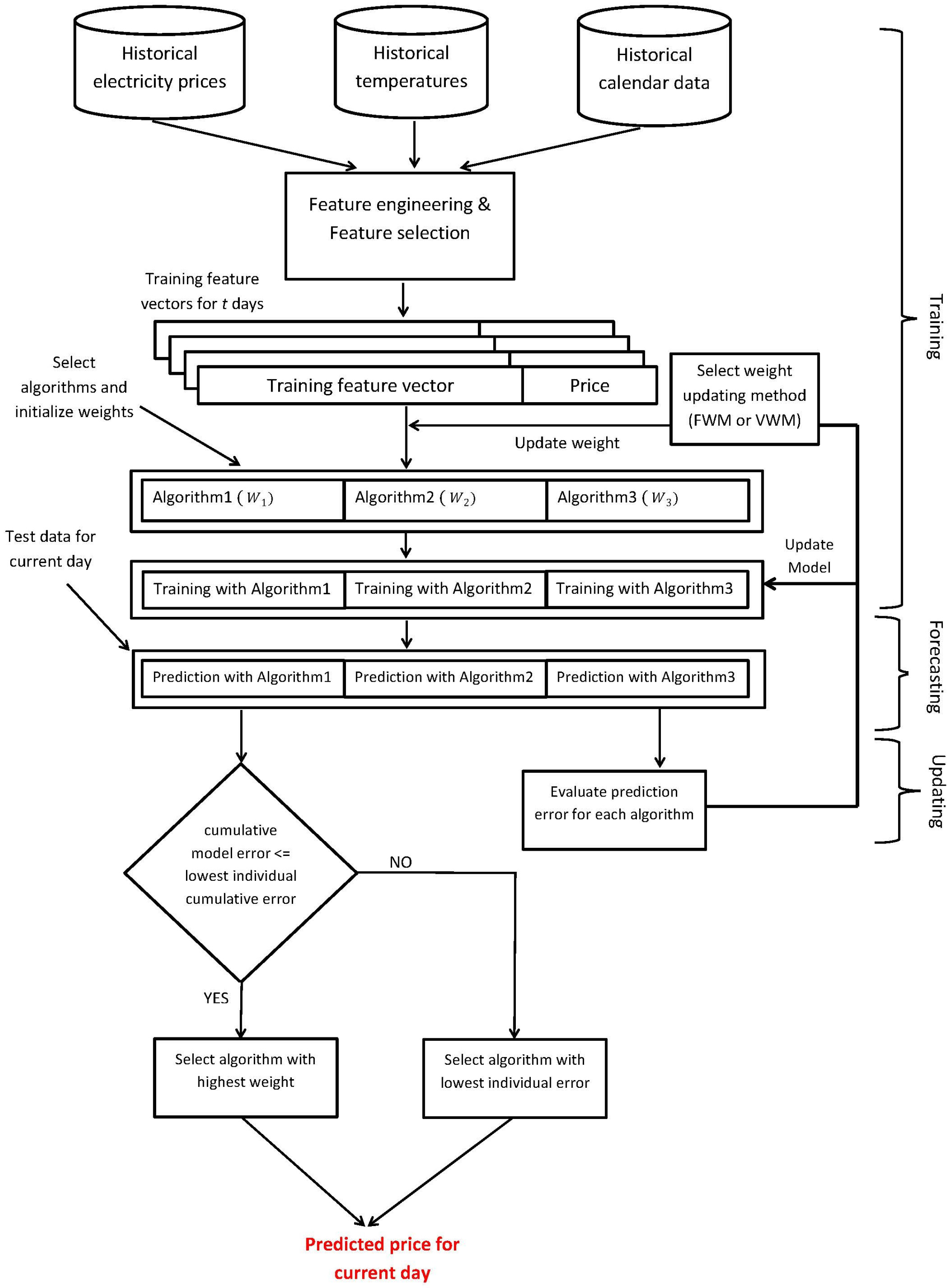
3.2. Model Architecture

The proposed model for electricity price prediction is presented in Figure 1. We have to recruit prediction algorithms that exhibit promising results when utilized separately to participate in our ensemble model. Here, we show three participating algorithms for demonstration purposes (in theory, any number of different algorithms can be used under this model depending on the processing power and time available). The proposed model performs feature engineering on the price data along with the corresponding temperature and calendar data collected from a de-regulated electricity market, which is followed by feature selection, learning, predicting and model updating steps.

All of the participating algorithms will generate predictions, but the actual decision will be made by the algorithm whose performance was best recently in the previous days. On the first day of the model deployment, the expert algorithm will be chosen randomly. From the second day onward, for each hour of the day, the performance of each algorithm will be evaluated, and the best algorithm will be chosen based on the past prediction accuracy. The best predictor will be the expert predictor, whose predicted value for the next day will be the decisive value. At the end of each day when the actual price becomes available, every algorithm will analyze its own performance for that day. If the performance is within the range of the threshold, the models are maintained. Otherwise, the models are updated by re-training them with all of the available data up to date. The proposed ensemble models, using fixed weights and varying weights respectively, are described in Algorithms 1 and 2.

It should be noted that both algorithms are designed for each individual hour of the day. Therefore, for each algorithm, we need to run 24 separate instances of it to forecast the electricity prices for 24 h.

3.2.1. Algorithm 1: Fixed Weight Method

The Fixed Weight Method (FWM) is described in Algorithm 1. Briefly, FWM is initialized by assigning a weight of zero to all participating algorithms, except for one randomly-chosen expert algorithm, whose weight is set to one. Models for each participating algorithm are then built using the training dataset and are used to predict the target electricity prices for the unseen test data. Once we obtain the prediction from each model, the constraint in Equation (4) is checked as a fallback procedure, and the final predicted value is decided. Then, the weight of each participating algorithm is updated based on the respective prediction accuracy. The weight for the model with the highest prediction accuracy is set to one, and zero is assigned to the weights of the rest of the models. The model with weight equal to one will be the expert model for the next day. If the performance of the expert model is below that of an individual model acting alone, a re-train signal is sent to the system, which will initiate the retraining of all of the individual models. Newly built models will replace the old models, but will maintain the weights of the previous models.

Algorithm 1 Fixed weight method ($TrainSet[1..t]$, $TestSet[1..m]$)

1: choose the set A of n participating algorithms: $A=\{a_1,a_2,a_3,\dots ,a_n\}$ 2: $\widehat{A}\leftarrow []$;    /* initialize list of experts */ 3: $e\leftarrow random(1..n)$; $W_e\leftarrow 1$;    /* randomly select an algorithm as expert and assign its weight as 1 */ 4: for $i\leftarrow 1$ to n do 5:   if $i\ne e$ then 6:       $W_i\leftarrow 0$;    /* initialize weights of all algorithms except expert’s as 0 */ 7:   end if 8:   $m{o}_i\leftarrow Train(a_i,TrainSet[1..t])$;    /* build prediction model $m{o}_i$ by training algorithm $a_i$ using data in the training set for days $1..t$ */ 9:   $CumuError[i]\leftarrow 0$;    /* initialize cumulative prediction error of all algorithms as 0 */ 10: end for 11: $ExpertCumuError\leftarrow 0$;    /* initialize cumulative prediction error of list of experts as 0 */ 12: $retrain\leftarrow$ FALSE; 13:   14: for $j\leftarrow 1$ to m do 15:   /* for all m number of days in $TestSet$, do the following three steps */ 16:   17:   /* Step 1: carrying out prediction */ 18:   for $i\leftarrow 1$ to n do 19:       /* apply prediction model $m{o}_i$ of algorithm $a_i$ using data in the training set plus those in the testing set up until previous day */ 20:       $P_{a_i}^{\prime }\leftarrow GetPrediction(m{o}_i,a_i,TrainSet\cup TestSet[1..j-1])$; 21:       if $W_i=1$ then 22:             $\widehat{a}\leftarrow a_i$;    /* if weight is 1, then it is the current expert */ 23:             add $\widehat{a}$ to list $\widehat{A}$;    /* insert the current expert into list of experts */ 24:             $PredictedPrice\leftarrow P_{\widehat{a}}^{\prime }$;    /* tentatively, predicted price will be output of the current expert */ 25:       end if 26:   end for 27:    28:   /* Step 2: fallback procedure and reporting */ 29:   $l\leftarrow {arg\; min}_{i=1..n}CumuError[i]$;    /* l is index of algorithm with lowest cumulative error */ 30:   if $CumuError[l]<ExpertCumuError$ then 31:       $PredictedPrice\leftarrow P_{a_l}^{\prime }$;    /* take algorithm l’s output instead of expert algorithm’s */ 32:       $retrain\leftarrow$ TRUE;    /* all models must be updated later */ 33:   end if 34:   report $PredictedPrice$;    /* report predicted price for j-th day as our output */ 35:    36:   /* Step 3: prediction error calculation and updating — after actual price P of day j is known */ 37:   $E_{\widehat{a}}\leftarrow |P_{\widehat{a}}^{\prime }-P|$;    /* calculate expert algorithm’s prediction error */ 38:   $ExpertCumuError\leftarrow ExpertCumuError+E_{\widehat{a}}$; 39:   for $i\leftarrow 1$ to n do 40:       $E_{a_i}\leftarrow |P_{a_i}^{\prime }-P|$;    /* calculate all algorithms’ prediction errors */ 41:       $CumuError[i]\leftarrow CumuError[i]+E_{a_i}$; 42:   end for 43:   $W_e\leftarrow 0$;    /* reset weight of old expert to 0 */ 44:   $e\leftarrow {arg\; min}_{i=1..n}{P}_{a_i}^{\prime }$;    /* select algorithm with lowest error for j-th day as new expert for $(j+1)$-th day */ 45:   $W_e\leftarrow 1$;    /* set weight of new expert as 1 */ 46:   /* re-train models if required */ 47:   if $retrain=$ TRUE then 48:       for $i\leftarrow 1$ to n do 49:             $m{o}_i\leftarrow Train(a_i,TrainSet\cup TestSet[1..j])$;    /*update all models using the latest available data till now */ 50:       end for 51:       $retrain=$ FALSE;    /* reset $retrain$ flag */ 52:   end if 53: end for

3.2.2. Algorithm 2: Varying Weight Method

Algorithm 2 describes the steps for the Varying Weight Method (VWM). VWM follows a similar approach as proposed in FWM, with few changes in updating the weight of participating algorithm. In this model, the weight of each participating algorithm varies based on the prediction accuracy achieved by the respective algorithm in all of the previous predictions made by it, whereas in FWM, the weight of the algorithm is either zero or one based on its previous day performance. At the beginning, the weight for all participating algorithms is set to one, and randomly, one algorithm is chosen to be the expert algorithm for the first day. These models are used to predict the electricity prices for the unseen test data. Once we obtain the prediction value from each model and come to know the actual price, we evaluate the performance of each model and update the weight based on the function of their prediction accuracy and learning rate λ. The algorithm with the highest accuracy (lowest prediction error) will have its weight increased, and the other algorithms with lower accuracy will have their weight decreased based on the prediction accuracy achieved by them. The main benefit of this model is that it considers the individual prediction error value when updating the weight. Therefore, the weight of any algorithm is dependent on the cumulative error and number of times it has been the best predictor.

3.3. Data Preprocessing

As presented in Figure 1, we need to perform feature engineering and feature selection prior to carrying out model building and prediction themselves.

3.3.1. Feature Engineering

The electricity market data follow a time series pattern and provide the information about the daily electricity prices over a period of time. The information in its raw form does not contain any specific features (attributes) that can be used in electricity price prediction. Therefore, from the time series data, we need to generate relevant features to be used in prediction models as an input. Previous research works have shown that prediction models are often affected by higher variance in time series data. Thus, feature generation, also known as feature engineering, is one of the important aspects in building the prediction model, where the features are carefully created to reduce over-fitting of the model and accurately capture the target value. In our previous work, we have shown that generating relevance features from single or a few sources improves the prediction accuracy of the model by a significant margin [12]. In this research, we have engineered 47 different features to capture various hidden trends in the electricity market.

In order to predict the hour h’s electricity price, we extract the hourly price data for the past 24 h ($h-1$–$h-24$) window, yielding 24 different features. The features that can best represent the short-term trend in the electricity market are the previous 24 h data, as observed in [47]. These data provide us a good insight for short-term trends, but fail to capture seasonal and long-term trends. In order to build a robust prediction model, both short and long term and the seasonal effect should be captured efficiently. A sudden high fluctuation in electricity price might occur due to the seasonal behavior and other factors. In order to capture these uncertain behaviors in electricity price, we created putatively relevant features based on a historical time series electricity price dataset. Therefore, 20 additional features, like last year same day same hour price, last year same day same hour price fluctuation, last week same day same hour price, last week same day price fluctuation, etc., were created.

In order to achieve an even better forecasting accuracy, we also introduce various features that are not directly associated with price data. We explore various other factors that can affect the electricity load and the price of the market. We have found that according to [7], the temperature, the day of the week and the occurrence of holidays can all affect the electricity load and price. Therefore, we also incorporate these three non-price features into our generated feature set. For the temperature features, we use historical and forecasted temperature data provided by Weather Underground [48]. For the holiday data, we use predefined holiday information in the geographical area of the target electricity market.

Algorithm 2 Varying weight method ($TrainSet[1..t]$, $TestSet[1..m]$, λ)

1: choose the set A of n participating algorithms: $A=\{a_1,a_2,a_3,\dots ,a_n\}$ 2: $\widehat{A}\leftarrow []$;    /* initialize list of experts */ 3: $e\leftarrow random(1..n)$;    /* randomly select an algorithm as expert */ 4: for $i\leftarrow 1$ to n do 5:   $W_i\leftarrow 1$;    /* initialize weights of all algorithms as 1 */ 6:   $m{o}_i\leftarrow Train(a_i,TrainSet[1..t])$;    /* build prediction model $m{o}_i$ by training algorithm $a_i$ using data in the training set for days $1..t$ */ 7:   $CumuError[i]\leftarrow 0$;    /* initialize cumulative prediction error of all algorithms as 0 */ 8: end for 9: $ExpertCumuError\leftarrow 0$;    /* initialize cumulative prediction error of list of experts as 0 */ 10: $retrain\leftarrow$ FALSE; 11:   12: for $j\leftarrow 1$ to m do 13:   /* for all m number of days in $TestSet$, do the following three steps */ 14:    15:   /* Step 1: carrying out prediction */ 16:   for $i\leftarrow 1$ to n do 17:       /* apply prediction model $m{o}_i$ of algorithm $a_i$ using data in the training set plus those in the testing set up until previous day */ 18:       $P_{a_i}^{\prime }\leftarrow GetPrediction(m{o}_i,a_i,TrainSet\cup TestSet[1..j-1])$; 19:   end for 20:   if $j\ne 1$ then 21:       $e\leftarrow {arg\; max}_{i=1..n}{W}_i$    /* if weight is the highest, then it is the current expert */ 22:   end if 23:   $\widehat{a}\leftarrow a_e$; add $\widehat{a}$ to list $\widehat{A}$;    /* insert the current expert into list of experts */ 24:    25:   $PredictedPrice\leftarrow P_{\widehat{a}}^{\prime }$;    /* tentatively, predicted price will be output of the current expert */ 26:    27:   /* Step 2: fallback procedure and reporting */ 28:   $l\leftarrow {arg\; min}_{i=1..n}CumuError[i]$;    /* l is index of algorithm with lowest cumulative error */ 29:   if $CumuError[l]<ExpertCumuError$ then 30:       $PredictedPrice\leftarrow P_{a_l}^{\prime }$;    /* take algorithm l’s output instead of expert algorithm’s */ 31:       $retrain\leftarrow$ TRUE;    /* all models must be updated later */ 32:   end if 33:   report $PredictedPrice$;    /* report predicted price for j-th day as our output */ 34:    35:   /* Step 3: prediction error calculation and updating — after actual price P of day j is known */ 36:   $E_{\widehat{a}}\leftarrow |P_{\widehat{a}}^{\prime }-P|$;    /* calculate expert algorithm’s prediction error */ 37:   $ExpertCumuError\leftarrow ExpertCumuError+E_{\widehat{a}}$; 38:   for $i\leftarrow 1$ to n do 39:       $E_{a_i}\leftarrow |P_{a_i}^{\prime }-P|$;    /* calculate all algorithms’ prediction errors */ 40:       $CumuError[i]\leftarrow CumuError[i]+E_{a_i}$; 41:   end for 42:   $s\leftarrow {arg\; min}_{i=1..n}{E}_{a_i}$    /* s is index of algorithm with smallest prediction error for current day j*/ 43:   /* update weights */ 44:   for $i\leftarrow 1$ to n do 45:       if $i=s$ then 46:             $W_i\leftarrow W_i\times (E_{a_i}\times \lambda )$    /* increase weight of algorithm $a_i$ by factor of λ and $E_{a_i}$ */ 47:       else 48:             $W_i\leftarrow W_i/(E_{a_i}\times \lambda )$    /* decrease weight of algorithm $a_i$ by factor of λ and $E_{a_i}$ */ 49:       end if 50:   end for 51:   /* re-train models if required */ 52:   if $retrain=$ TRUE then 53:       for $i\leftarrow 1$ to n do 54:             $m{o}_i\leftarrow Train(a_i,TrainSet\cup TestSet[1..j])$;    /*update all models using the latest available data till now */ 55:       end for 56:       $retrain=$ FALSE;    /* reset $retrain$ flag */ 57:   end if 58: end for

It should be noted that oil and gas prices and other factors, like load and types of resources used for electricity generation, might also affect the pricing. However, for the three target markets in out studies (namely, New York, Australia and Spain), these data are not easily accessible to us, and we leave them to be considered in our future work.

Normalization is one of the best approaches to deal with the input data where the attributes are of different measurements and scales. In our case, as we use various input data with different scales, we need to normalize all 47 attributes to achieve consistency. We use the mapminmax function in MATLAB [49] to normalize the input attributes into the range $(-1.0,1.0)$.

3.3.2. Feature Selection

Though 47 features were created using the historical electricity price, calendar and weather data, using all of the created features for building the model poses the threat of over-fitting. All of the generated features are analyzed to remove redundant, irrelevant and loosely-coupled features. Thus, the feature selection process is used to select the most relevant features from the original feature set.

Feature selection is a crucial step in building a robust prediction model. Here, we utilize the wrapper method [50] using WEKA [51] for subset selection from a pool of features. A wrapper involves a search algorithm for finding the optimal subset of features in the feature space and evaluating the subset using the learning algorithm. Using cross-validation, it evaluates the estimated accuracy obtained from the learning algorithm by adding or removing features from the features subset in hand. In our case, we use the Artificial Neural Network (ANN) as the learning algorithm; 10-fold cross-validation is carried out for the training set.

In selecting the optimal feature set, among the 47 features, the wrapper method is applied to the 23 features apart from those for the past 24 h. Technically, the resultant training accuracy may be less than the best possible accuracy since 24 features are omitted. However, due to the verified importance of the past 24 h data [47], we choose to exclude them for the sake of saving expensive computation of the wrapper process, whose running time cost is exponential to the number of input features.

The final feature set obtained for the New York (NYISO) dataset after the feature selection process is shown as an example in

Table 1. Selected features for the NYISO (New York Independent System Operator) dataset.

Attribute No.	Description	Notation
1–24	Previous 24 h’s prices	$p_{h-1}$ to $p_{h-24}$
25	Previous year same hour price	$p_{y-1}$
26	Previous year same day average price	$p_{avg(y-1)}$
27	Previous week same hour price	$p_{d-7}$
28	Previous hour price increase/decrease	$|p_{h-1}-p_{h-2}|$
29	Previous year same day, same hour, price increase/decrease	$|p_{{(y-1)}_h}-p_{{(y-1)}_{h-1}}|$
30	Temperature of the day	$T_d$
31	Day of the week	$W_d$
32	Holiday (Y/N)?	$H_d$

.

4. Experimental Setup

4.1. Data

We evaluated our proposed ensemble model by performing experiments with the dataset from three different deregulated electricity markets of New York (NYISO) [13], Australia (ANEM) [14] and Spain (OMEL) [15]. We selected data from these markets to compare the results of our proposed model with those in the previous works. As mentioned in [11], a vast amount of research has been carried out using the data from these markets. The NYISO electricity market contains data from various areas from New York and provides data for hourly electricity price. From NYISO, we selected “Capita” as the reference area to benchmark our results with those of the previous works [11,12]. ANEM represents the market clearing data in the Australian market since its deregulation with half hour resolution. Again, we selected the data from the “Queensland” area to be consistent with the experiments in those two previous works. Likewise, for the Spanish (OMEL) market, we also used the same data as those previous works.

4.2. Evaluation Metrics

Following are the performance measures used to validate our proposed model. These measures are used in order to facilitate direct comparison with the results obtained in the other similar studies.

Mean Error Relative to the mean actual price (MER):

$$MER=100\times \frac{1}{N}\sum _{i=1}^N\frac{|P_i-P_i^{\prime }|}{\overline{P}}$$

(5)

where $P_i$ defines the actual price and $P_i^{\prime }$ defines the predicted price. $\overline{P}$ is the mean price for the period of interest, and N is the number of predicted hours. This indicator is irrespective of the absolute values.

Mean Absolute Error (MAE):

$$MAE=\frac{1}{N}\sum _{i=1}^N|P_i-P_i^{\prime }|$$

(6)

The indicator is dependent on the absolute range of the electricity price.

Mean Absolute Percentage Error (MAPE):

$$MAPE=100\times \frac{1}{N}\sum _{i=1}^N\frac{|P_i-P_i^{\prime }|}{P_i}$$

(7)

This indicator is irrespective of the absolute values. If the range of the electricity price is vast, a prediction may give a high MAE value, but a low MAPE.

5. Experimental Results

Two sets of experiments (Experiments I and II) were performed using two different time periods, 2004–2006 (on the NYISO, ANEM and OMEL datasets) and 2008–2012 (on the NYISO and ANEM datasets only), respectively.

5.1. Experiment I: 2004–2006

In Experiment I, the NYISO, ANEM and OMEL datasets for the time period of 2004–2006 are used. For all of the datasets, data from March 2004–March 2006 were used as the training set and April 2006–December 2006 as the testing set. We use the exact same experimental protocol as in Martínez-Álvarez et al. [11]. The following five methods are compared.

• Ensemble learning using the Fixed Weight Method (FWM) (Algorithm 1) using three participating machine learning algorithms: Artificial Neural Network (ANN), Support Vector Regression (SVR) and Random Forest (RF) [52],
• Ensemble learning using the Varying Weight Method (VWM) (Algorithm 2) using the same participating algorithms as in FWM,
• Artificial Neural Network only (ANN-only) (published results as presented in our previous work [12]),
• Pattern Sequence-based Forecasting (PSF) (published results as presented in Martínez-Álvarez et al. [11]) and
• Autoregressive Integrated Moving Average (ARIMA) [10] (Note: the auto.arima() function in R’s [53] Forecast package is used.)

5.1.1. Experiment I-A: NYISO Dataset

Table 2. MER (Mean Error Relative to the mean actual price), MAE and MAPE evaluation metrics for the NYISO market for the year 2006 (Experiment I-A). VWM, Varying Weight Method; FWM, Fixed Weight Method; PSF, Pattern Sequence-based Forecasting.

NYISO (2006)
Month	MER (%)					MAE (USD/MWh)					MAPE (%)
	VWM	FWM	ANN-Only	PSF	ARIMA	VWM	FWM	ANN-Only	PSF	ARIMA	VWM	FWM	ANN-Only	ARIMA
January				4.45	6.51				2.25	4.75				6.17
February				5.53	6.28				3.02	4.23				5.97
March				6.30	6.87				3.97	3.80				5.95
April	3.61	3.79	3.99	4.94	5.56	2.23	2.22	2.34	3.51	3.32	3.66	3.82	4.02	5.67
May	2.67	2.79	2.94	7.59	4.92	1.62	1.64	1.72	4.63	2.73	3.02	3.07	3.23	5.09
June	3.32	3.47	3.65	3.34	4.70	1.96	2.03	2.14	2.31	2.73	3.64	3.64	3.83	5.02
July	3.95	3.89	4.09	3.93	5.31	2.22	2.28	2.40	2.28	3.39	3.82	3.75	3.95	5.56
August	4.56	4.58	4.82	5.37	5.17	2.59	2.68	2.82	3.49	3.55	3.80	3.76	3.96	5.25
September	2.64	2.72	2.86	6.24	4.83	1.58	1.59	1.68	4.49	2.24	3.27	3.42	3.60	5.15
October	3.05	3.19	3.36	7.43	6.18	1.78	1.87	1.97	4.23	3.23	3.85	3.89	4.09	6.35
November	5.24	5.25	5.53	5.19	9.64	2.77	2.90	3.05	3.53	6.06	4.76	4.91	5.17	9.04
December	5.70	5.61	5.90	6.04	12.42	3.07	3.02	3.18	3.08	5.79	5.55	5.46	5.75	9.43
Mean	3.86	3.92	4.13	5.53	6.53	2.20	2.25	2.37	3.40	3.82	3.93	3.97	4.18	6.22
SD	1.10	1.03	1.09	1.29	2.29	0.52	0.53	0.55	0.84	1.19	0.77	0.75	0.79	1.47

Notes: (1) For the NYISO dataset, The results for the period January–March 2006 cannot be presented for VWM, FWM and ANN-only because the feature vectors of their corresponding training data during the period of January–March 2005 cannot be constructed. Construction of those training feature vectors in turn requires the data before March 2004, which is not readily available to us. For PSF and ARIMA, such a feature vector construction is not required, and neither are the data before March 2004. (2) MAPE results for PSF are not presented because it was not used as an evaluation criterion in [11]. (3) The Standard Deviation (SD) results provided here are computed using the stdev (estimated standard deviation based on a sample) function in Microsoft Excel. They are different from the ones reported in [11] and [12], which are computed by a different standard deviation function.

shows the MER (Equation (5)), MAE (Equation (5)) and MAPE (Equation (7)) of the four methods for New York (NYISO) data for the testing period of the year 2006. We can see that the results obtained from FWM (VWM in the brackets) have average MER of 3.92% (3.86%) with the SD (Standard Deviation) of 1.03 (1.10), MAE of USD 2.25/MWh (USD 2.20/MWh) with SD of 0.53 (0.52) and MAPE of 3.97% (3.93%) with SD of 0.75 (0.77). The worst month is December 2006, where MER is 5.61% (5.70%), MAE is 3.02 (3.07) and MAPE is 5.46% (5.55%).

For both FWM and VWM, the ANN predictor appears to dominate the other algorithms where more than 60% of its predictions were selected as the final prediction in both cases. Generally, VWM offers slightly better results than FWM with the improvements (decreases in error) of 0.06% of MER, USD 0.05/MWh of MAE and 0.04% of MAPE.

5.1.2. Experiment I-B: ANEM Dataset

The Australian (ANEM) dataset is particularly challenging. It is highly volatile with a large number of unexpected abnormalities and outliers. There were large fluctuations in the electricity prices with the highest price of AUD 9739/MWh in January 2006 and the lowest value of AUD 7.81/MWh in February 2004. The variance and skewness for each market datum will be discussed in the following Section 6.

Due to these highly fluctuating values and outliers, forecasted price for this market has a high range of error. From

Table 3. MER, MAE and MAPE evaluation metrics for the ANEM (Australian Energy Market Operator) market for the year 2006 (Experiment I-B).

ANEM (2006)
Month	MER (%)					MAE (AUD/MWh)					MAPE (%)
	VWM	FWM	ANN-Only	PSF	ARIMA	VWM	FWM	ANN-Only	PSF	ARIMA	VWM	FWM	ANN-Only	ARIMA
January	14.03	16.43	13.96	5.80	42.92	4.61	5.32	4.66	1.51	11.43	12.71	15.20	13.34	49.17
February	7.04	7.93	7.26	8.59	55.51	2.37	2.57	2.42	5.15	36.85	6.98	7.67	7.19	55.21
March	4.44	4.86	4.59	7.84	37.79	1.47	1.57	1.53	1.73	7.37	4.75	5.22	4.79	37.87
April	5.53	5.56	5.60	9.92	40.01	1.78	1.80	1.87	1.98	8.32	5.56	5.96	5.82	42.81
May	10.09	10.03	10.07	12.85	49.25	3.22	3.24	3.36	3.21	11.72	9.43	9.27	9.59	44.43
June	11.20	12.01	11.00	22.04	27.23	3.72	3.89	3.67	6.81	8.56	7.54	9.01	7.85	28.09
July	17.14	18.47	17.97	17.11	77.21	6.02	5.98	5.99	8.16	37.33	13.15	14.53	13.84	41.73
August	11.12	12.18	11.28	11.71	25.94	3.81	3.94	3.76	3.32	7.78	7.52	9.13	7.55	25.56
September	8.36	9.32	8.77	8.23	24.20	2.83	3.02	2.93	2.34	6.86	7.08	7.03	7.03	27.42
October	5.59	6.15	5.70	7.66	25.47	1.89	1.99	1.90	1.92	6.47	5.23	5.77	5.40	29.92
November	10.41	11.61	10.59	6.76	28.19	3.54	3.76	3.53	2.09	8.88	9.11	9.18	9.25	27.00
December	5.94	6.15	6.12	6.42	39.70	2.00	1.99	2.04	1.41	7.26	6.06	6.41	6.35	41.44
Mean	9.24	10.06	9.41	10.41	39.45	3.11	3.25	3.14	3.30	13.24	7.93	8.70	8.17	37.55
SD	3.83	4.32	3.92	4.87	15.61	1.34	1.40	1.31	2.23	11.26	2.74	3.23	2.90	9.82

, we can see that the performance FWM (VWM in the brackets) of on ANEM data is 10.06% (9.24%) of average MER with SD of 4.32 (3.83), AUD 3.25/MWh (AUD 3.11/MWh) MAE with SD of 1.40 (1.34) and 8.70% (7.93%) MAPE with SD of 3.23 (2.74).

Bad performances are observed for the months of January, June, July and August 2006. The worst performance of 18.47% (17.14%) MER and 14.53% (13.15%) MAPE are obtained July 2006. The best performance of 4.86% (4.44%) MER and 5.22% (4.75%) MAPE are in the month of March 2006.

Though the results on this ANEM dataset by FWM and VWM have higher error percentages than those on the previous NYISO dataset, the performance of VWM is still better than those of the other methods (ANN-only and PSF) on the same dataset. On the other hand, the accuracy of FWM is found to be slightly lower than that of the ANN-only method, but still higher than that of PSF. The final predictions for ANEM dataset also follow the same trend as in the NYISO dataset where a majority of the predictions were based on ANN as the expert algorithm for both FWM and VWM.

5.1.3. Experiment I-C: OMEL Dataset

The results obtained from the Spanish (OMEL) market are shown in

Table 4. MER, MAE and MAPE evaluation metrics for the Spanish OMEL (Operador del Mercado Ibérico de Energía, Polo Español, S.A.) market for the year 2006 (Experiment I-C).

OMEL (2006)
Month	MER (%)					MAE (EURc/kWh)					MAPE (%)
	VWM	FWM	ANN-Only	PSF	ARIMA	VWM	FWM	ANN-Only	PSF	ARIMA	VWM	FWM	ANN-Only	ARIMA
January	5.91	5.65	6.00	7.26	8.31	0.40	0.36	0.40	0.53	0.61	5.00	4.56	5.07	8.91
February	5.20	5.34	5.25	4.93	8.05	0.34	0.35	0.35	0.36	0.58	3.49	3.88	3.66	8.02
March	5.05	5.48	5.28	5.88	10.80	0.34	0.35	0.35	0.43	0.55	6.28	6.33	6.19	11.26
April	5.68	6.11	5.90	3.62	11.44	0.39	0.39	0.39	0.28	0.58	5.55	5.88	5.73	10.67
May	5.88	5.60	6.00	8.11	10.42	0.40	0.36	0.40	0.64	0.51	5.88	5.69	6.11	10.38
June	5.12	5.36	5.14	3.76	8.92	0.33	0.35	0.34	0.29	0.42	5.05	5.68	5.27	8.47
July	4.68	4.59	4.59	4.30	8.19	0.29	0.30	0.30	0.33	0.41	4.59	4.52	4.55	8.16
August	5.10	5.07	5.17	5.37	9.36	0.33	0.33	0.34	0.42	0.43	5.50	5.39	5.57	8.78
September	5.61	5.44	5.66	6.41	10.64	0.36	0.35	0.37	0.50	0.56	5.36	5.03	5.42	10.06
October	6.04	5.78	6.08	7.89	11.87	0.41	0.37	0.40	0.58	0.53	6.31	6.23	6.64	10.60
November	3.83	4.10	3.94	8.30	7.53	0.25	0.27	0.26	0.64	0.28	7.13	7.91	7.25	10.61
December	5.06	5.50	5.04	8.02	12.06	0.33	0.36	0.33	0.59	0.41	7.33	7.94	7.61	12.32
Mean	5.26	5.34	5.34	6.15	9.80	0.35	0.34	0.35	0.47	0.49	5.62	5.75	5.76	9.85
SD	0.62	0.54	0.64	1.76	1.60	0.05	0.03	0.04	0.13	0.10	1.07	1.25	1.11	1.36

. We can see that the average MER of FWM (VWM in the brackets) is 5.34% (5.26%) with SD of 0.54 (0.62), which indicates that the monthly errors are not much different from the average error. MAE for the Spanish data is EURc 0.34/kWh (EURc 0.35/kWh) with the SD of 0.03 (0.05) and MAPE of 5.75% (5.62%) with SD of 1.25 (1.07). MAE for the OMEL dataset is very low compared to other markets because the prices are in a different unit of measurement, which is EUR cent per kWh instead of USD/AUD per MWh in the NYISO/ANEM datasets.

It can also be observed that, unlike the previous two cases of NYISO and ANEM, VWM is not always better than FWM for all three evaluation criteria. Whilst VWM is slightly better than FWM in terms of the average MER and MAPE, it is slightly worse than FWM in terms of MAE.

5.2. Experiment II: 2008–2012

To further verify these encouraging results, a second set of experiments were performed using the more recent dataset. Electricity price data from the June 2008–May 2011 period were extracted from the NYISO and ANEM datasets and used as the training set, while data from June 2011–May 2012 were used as the testing set (note: the OMEL dataset is not available for the period 2008–2012, and neither are the experimental results of PSF for that time period). Therefore, only FWM (with ANN, SVR and RF participating algorithms), VWM (with the same participating algorithms), ANN-only and ARIMA are compared. It is observed that the results of our proposed model for this Experiment II are even slightly better than those in Experiment I.

5.2.1. Experiment II-A: NYISO Dataset

From

Table 5. MER, MAE and MAPE evaluation metrics for the NYISO market for the years 2011–2012 (Experiment II-A).

NYISO (2011–2012)
Month	MER (%)				MAE (USD/MWh)				MAPE (%)
	VWM	FWM	ANN-Only	ARIMA	VWM	FWM	ANN-Only	ARIMA	VWM	FWM	ANN-Only	ARIMA
June 2011	4.25	4.24	4.27	5.42	1.92	1.97	2.01	2.36	5.19	5.32	4.31	5.19
July 2011	4.40	4.36	4.66	6.46	2.71	2.68	2.97	3.59	7.12	7.25	4.72	5.82
August 2011	3.39	3.34	3.54	5.04	1.50	1.48	1.56	2.21	3.87	3.99	3.51	5.13
September 2011	3.56	3.61	3.86	5.23	1.38	1.38	1.47	2.05	3.72	3.73	3.76	5.41
October 2011	3.49	3.50	3.55	5.98	1.33	1.32	1.33	2.31	3.60	3.56	3.48	5.89
November 2011	3.57	3.56	3.61	6.73	1.31	1.28	1.30	2.38	3.41	3.47	3.62	6.36
December 2011	3.73	3.80	4.01	7.97	1.35	1.36	1.44	2.81	3.68	3.68	4.16	6.98
January 2012	4.82	4.87	4.92	9.72	2.19	2.15	2.32	3.90	5.71	5.82	5.14	8.26
February 2012	3.22	3.25	3.70	6.67	1.06	1.05	1.20	2.03	2.84	2.83	3.81	6.05
March 2012	4.74	4.76	4.83	8.44	1.27	1.29	1.31	2.25	3.48	3.48	4.86	7.93
April 2012	3.84	3.80	4.18	7.21	0.96	0.95	1.06	1.88	2.44	2.56	4.09	7.20
May 2012	3.22	3.23	3.45	5.41	0.84	0.83	0.88	1.54	2.18	2.25	3.27	5.80
Mean	3.85	3.86	4.05	6.69	1.48	1.49	1.57	2.44	3.94	3.99	4.06	6.34
SD	0.56	0.57	0.52	1.44	0.54	0.54	0.59	0.68	1.42	1.45	0.60	1.04

, we can see that the overall performances of both FWM and VWM for this 2008–2012 NYISO dataset are even slightly better than those for the Experiment I-A (NYISO’s 2004–2006 dataset) despite the fact that the 2008–2012 data contain many spikes and outliers. For this dataset, FWM (VWM in the brackets) provides average MER of 3.86% (3.85%) with SD of 0.57 (0.57), MAE of USD 1.48/MWh (USD 1.48/MWh) with SD 0.54 (0.54) and MAPE 3.99% (3.94%) with SD of 1.45 (1.42). Noticeable improvement can be observed in MAE with a decrease of USD 0.77/MWh (USD 0.72/MWh) when compared to Experiment I-A.

The worst forecasting results obtained were 4.87% (4.82%) of MER in January 2012, USD 2.68/MWh (USD 2.71/MWh) of MAE and 7.25% (7.12%) of MAPE both in July 2011. The main reason for the higher forecasting error in July 2011 and January was due to the higher numbers of spikes and outliers in those months in the New York market.

5.2.2. Experiment II-B: ANEM Dataset

The performances of FWM and VWM in this period for the ANEM dataset are noticeably better for those of Experiment I-B (ANEM’s 2004–2006 dataset). For this dataset, FWM (VWM in the brackets) provides average MER of 7.16% (6.98%) with SD of 3.83 (3.98), MAE of AUD 2.09/MWh (AUD 2.05/MWh) with SD 1.37 (1.36) and MAPE of 6.22% (6.16%) with SD of 3.01 (2.98). The improvements (deceases in error) over ANEM’s 2004–2006 dataset by FWM (VWM in the brackets) are 2.90% (2.26%) in MER, AUD 1.16/MWh (AUD 1.06/MWh) in MAE and 2.48% (1.77%) in MAPE.

There are also decreases in SD for both FWM and VWM, which indicate that the errors in the years 2011–2012 are lessdeviated from the mean error when compared to those for the years 2004–206 in the ANEM dataset.

The worst performance of FWM (VWM in the brackets) was in the months of January–March 2012 with 14.36% (13.72%) MER in February 2012. The best performance of 3.72% (3.66%) MER was in May 2012. The best and the worst MAPEs were 3.83% (3.76%) in May 2012 and 12.72% (12.61%) in February 2012, respectively.

6. Analyses and Discussions

6.1. Variance and Skewness vs. Accuracy

The statistical distributions of the price data can significantly affect the model’s prediction accuracy. In this section, we analyze different properties of the electricity price data for all three markets. One key aim is to find correlations between the data distribution and prediction error and to justify the requirement for an independent prediction model for each hour of the day as proposed in our approach. Figure 2 and Figure 3 show overall variance and average price for 2004–2006 and 2008–2012 training and testing data for all three electricity market along with average forecasting accuracy. From both figures, we can see that the NYISO and ANEM data are of high variance. However, when we compare the value with the respective average price, ANEM shows a higher variance in price with a lower average price.

Higher variance in price and higher deviation in hourly training and testing data might be the reason for higher error for ANEM’s 2004–2006 dataset as shown in Figure 2. From Figure 3, we can see for the 2008–2012 dataset, ANEM continues to have higher variance in the training and the testing data, but Figure 8 shows that the hourly variance deviation between the training and the testing data is less, which helps to lower the forecasting error for ANEM. In Figure 6, we can see that the OMEL dataset shows a different response to hourly variance in the dataset. As opposed to NYISO and ANEM, the OMEL 2004–2006 dataset is of a lower variance to average price ratio, but still, its prediction error is higher than that of NYISO. The main cause behind this prediction error is due to the presence of a few outliers, where the ratio between the maximum the the minimum electricity price is more than 1000 fold (the data values for the OMEL dataset in Figure 2 are proportionally adjusted to make them comparable to those of the other markets because, unlike the others, the OMEL market represents electricity price in Euro cent per kWh).

For every electricity market, if we inspect the variances in prices within the same market for different hours of the day, we can observe that there is a great fluctuation in variances. Figure 4, Figure 5 and Figure 6 show the hourly variance in 2004–2006 electricity price data for NYISO, ANEM and OMEL, respectively. Similarly, Figure 7 and Figure 8 show the hourly variance in 2008–2012 electricity prices for NYISO and ANEM, respectively. From these five figures, we can see that each market exhibits different distributions of data over different hours of the day. For example, if we look at Figure 5, we can see that the ANEM 2004–2006 dataset shows price variances ranging from 30–1400 AUD/MWh for the training dataset and from 32–1950 AUD/MWh for the testing dataset. We can see similar fluctuations in price variances for the NYISO and OMEL datasets, as well. These markets are also of different variances in price over hours of the day, but both the training and the testing data follow a similar trend. On the other hand, the ANEM market shows a large difference in the training vs. testing curves for the 2004–2006 dataset, but somewhat more consistent curves for the 2008–2012 dataset.

From Figure 9, we can see that the ANEM 2004–2006 dataset exhibits high skewness along with higher forecasting error when compared to NYISO and OMEL. This high skewness continues in the ANEM 2008–2012 dataset shown in Figure 10.

From all of the above observations, we can infer that electricity markets are of different price distributions, which are highly dependent on the hour of the day, with some hours having higher variance in price and some lower variance. This distribution is further influenced by the deployment of the smart grid, where the electricity price depends on various factors, like the load, user behavior, demand-response, etc. Under this circumstance, it very difficult to find an approach that can offer consistent performance over different electricity markets. This issue is somehow resolved by our proposed model, which provides flexibility on participating algorithms and tries to adapt to the changes in the data distribution. Our proposed model captures the variation in price with carefully-engineered features and builds varying forecasting models separately, one for each hour of the day. The model automatically adjusts itself to certain changes in the environment by evaluating the performance of the model at the end of each day and makes necessary adjustments if required.

6.2. Ensemble Model

Two different experiments were performed with different approaches (FWM and VWM) for updating the weights of the participating algorithms. From the results, we can see that the performance of VWM was slightly better than that of FWM. This was because in VWM, the weights are adjusted based on the prediction error, i.e., the change in weight is higher if the difference between the real and the predicted value is higher. Whereas in FWM, changes in weight do not depend on the level of accuracy of the algorithm, and it just looks at which algorithm performs the best. In VWM, each algorithm is evaluated based on all of its previous errors, which is directly correlated to the final prediction accuracy of the model. VWM is better (incurs less error) than FWM by 0.06%–0.18% of MER, 0.03–0.04 of MAE (USD/MWh, AUD/MWh or EURc/kWh) and 0.05%–0.24% of MAPE. Both approaches show high improvement in accuracy compared to our benchmark method (PSF) and some improvement over our previous work (ANN-only). During the experiments, no single scenario (models for each hour of the day and dataset) had the same expert throughout the test period. These periodic changes of expert show that all of the participating algorithms continually learn from the mistakes and adjust their parameters to capture the current price trends and external impact on prices, eventually showing their presence in the ensemble, i.e., being selected as an expert. Thus, the proposed ensemble approach was able to automatically create a tailored model for each scenario and achieved a higher accuracy.

Analyzing the results, among the three participating algorithms, we found the performance of ANN to be comparatively better than SVR and RF when the price is of higher fluctuation, whereas the performances of SVR and RF were better when the price is of lower fluctuation. ANN shows consistent performance with both VWM and FWM, whereas SVR fails to perform well in VWM, as the prediction error for SVR was very high during the peak price, which decreased the weight of SVR by a large margin. RF also shows consistent performance, but it also degrades in some cases of the peak price. In general, high and sudden variations in the electricity price, which are influenced by many unforeseen factors, cause degradation in performance of our ensemble model (both for VWM and FWM). We can see that our model’s performance for a few months is below its average performance due to many sharp price increases in those months.

6.3. Comparisons with ARIMA, PSF and ANN-Only Methods

To validate the performance of FWM and VWM, the results obtained were compared with those obtained using other methods, namely ARIMA, PSF and ANN-only.

6.3.1. Proposed Methods vs. ARIMA

Both FWM and VWM outperformed the standard time series forecasting method, ARIMA [10], by large margins in all five test cases, as shown in Table 2, Table 3, Table 4, Table 5 and

Table 6. MER, MAE and MAPE evaluation metrics for the ANEM market for the years 2011–2012 (Experiment II-B).

ANEM (2011–2012)
Month	MER (%)				MAE (AUD/MWh)				MAPE (%)
	VWM	FWM	ANN-Only	ARIMA	VWM	FWM	ANN-Only	ARIMA	VWM	FWM	ANN-Only	ARIMA
June 2011	4.11	4.32	4.60	11.08	1.15	1.20	1.28	2.81	4.42	4.34	4.62	10.99
July 2011	6.85	7.01	7.46	15.63	1.98	1.95	2.07	4.13	6.59	6.52	6.94	15.26
August 2011	4.73	4.76	5.06	9.60	1.30	1.32	1.41	2.77	4.07	4.18	4.44	9.29
September 2011	4.05	4.17	4.43	8.56	1.13	1.16	1.23	2.35	4.02	3.99	4.25	8.61
October 2011	4.19	4.36	4.64	7.87	1.15	1.21	1.29	2.15	4.08	4.29	4.57	7.98
November 2011	6.90	6.89	7.33	12.61	1.88	1.91	2.03	3.95	5.52	5.73	6.10	11.63
December 2011	4.65	4.71	5.01	7.18	1.30	1.31	1.39	1.84	4.38	4.43	4.72	7.88
January 2012	12.53	13.05	13.88	24.09	2.97	3.10	3.30	6.82	8.58	8.54	9.09	19.20
February 2012	13.72	14.36	15.28	24.58	5.29	5.29	5.63	7.44	12.61	12.72	13.53	19.84
March 2012	13.04	13.17	14.01	24.47	4.04	4.17	4.44	6.75	10.96	11.17	11.89	19.98
April 2012	5.40	5.34	5.68	9.27	1.42	1.48	1.58	2.71	4.93	4.90	5.21	9.05
May 2012	3.66	3.72	3.95	7.93	1.00	1.03	1.10	2.03	3.76	3.83	4.07	8.32
Mean	6.98	7.16	7.61	13.57	2.05	2.09	2.23	3.81	6.16	6.22	6.62	12.34
SD	3.83	3.98	4.24	6.92	1.36	1.37	1.46	2.05	2.98	3.01	3.20	4.88

. It can be observed that ARIMA performs quite poorly, particularly on the ANEM dataset (2004–2006), which contained some huge price spikes.

6.3.2. Proposed Methods vs. PSF

In [11], Pattern Sequence-based Forecasting (PSF) was reported to have outperformed other contemporary works, namely ARIMA, naive Bayes, ANN (this ANN implementation is distinct from our previous work (ANN-only) [12] because of different feature engineering approaches), WNN (Weighted Nearest Neighbor) [54], the Structural model (STR) [55] and other mixed models. As testing was performed on the 2004–2006 data from all three markets in the PSF paper, we also perform the testing on same data and achieve the better results shown in Table 2, Table 3 and Table 4.

It can be observed that FWM (VWM in brackets) forecasts with 1.61% (1.67%) improved accuracy in terms of MER in the NYISO dataset. There are improvements (i.e., decreases in error) of average MER by 0.35% (1.17%) for the ANEM dataset and 0.81% (0.89%) for the OMEL dataset.

Similar accuracy improvements by FWM/VWM over PSF can be seen for the MAE criterion, as well. FWM (VWM in brackets) offers higher accuracy over PSF in average MAE by USD 1.15/MWh (USD 1.20/MWh), AUD 0.19/MWh (AUD 0.05/MWh) and EURc 0.13/kWh (EURc 0.12/kWh) for NYISO, ANEM and OMEL respectively.

Furthermore, we claim that the performances of the two proposed methods are more stable as the standard deviations of both the MER and MAE obtained by FWM/VWM are smaller than those obtained by PSF.

6.3.3. Proposed Methods vs. ANN-Only

Finally, we compare the proposed techniques with an existing ANN-only method, which we had presented in an earlier work [12] and that was shown to produce higher forecasting accuracy than PSF.

For the 2004–2006 datasets, both FWM and VWM provided better results than ANN-only for NYISO. FWM (VWM in the brackets) provides improvements of 0.21% (0.27%) in MER, USD 0.12/MWh (USD 0.17/MWh) in MAE and 0.21% (0.25%) in MAPE.

For ANEM (2004–2006), FWM turns out to be inferior to ANN-only by $-0.65$% MER, $-0.11$AUD/MWh MAE and $-0.53$% MAPE. However, VWM is still better than ANN-only by 0.17% MER, AUD 0.03/MWh MAE and 24% MAPE. For the OMEL dataset, both FWM and VWM are slightly better than or perform equally as ANN-only.

The improvements of FWM (VWM in the brackets) for OMEL (2004–2006) are 0% (0.08%) MER, EURc 0/kWh (EURc0.01/kWh) MAE and 0.01% (0.14%) MAPE. In terms of SD, FWM provides smaller SD values than ANN-only in five out of nine test cases (i.e., 3 datasets × 3 evaluation criteria), and VWM provides smaller SD than ANN-only in six out of nine test cases.

Similar trends are also observed for the NYISO and ANEM (2008–2012) datasets, thus confirming the effectiveness of the proposed VWM and FWM methods.

7. Conclusions

Electricity price forecasting in the deregulated electricity market is essential to facilitate the decision making processes of the stakeholders. Although extensive research has been carried out in this field, the accuracy of existing techniques is not consistently high, especially in volatile and complex market conditions. In this paper, an ensemble-based model that combined three different electricity price forecasting algorithms was proposed. Also presented were two different approaches for updating the weights of the participating algorithms and for selecting the final expert algorithm, whose prediction will be adopted as the final model prediction.

Comparative experimental studies were performed to benchmark the proposed model against a number of existing techniques; these were: ARIMA, which is the standard statistical time series model, PSF, a recent highly-regarded method, which was superior to many other existing methods, as well as a method which we had presented in an earlier work, which used a single ANN regressor. The experiments were conducted on data collected from three different electricity markets and for time periods ranging from 2006–2012, and the results showed that our model outperforms the conventional approaches and produces robust and accurate forecasts, even with a variety of different datasets and over a long period of time.

However, there is still room for improvement, and we plan to carry out the following tasks in the future:

• Further testing on other electricity markets.
• Inclusion of other exogenous features, such as oil/gas prices, electricity generation modalities, etc.
• Incorporation of features to model dynamics associated with the smart grid, like demand response and load balancing.
• Development of better weighting schemes to further improve the accuracy.