Abstract
In a carbon-constrained world, natural gas with low emission intensity plays an important role in the energy consumption area. Energy consumers and distribution networks are linked via energy hubs. Meanwhile, reconfiguration that optimizes operational performance while maintaining a radial network topology is a worldwide technique in the electricity distribution system. To improve the overall efficiency of energy infrastructure, the expansion of electricity distribution lines and elements within energy hubs should be co-planned. In this paper, the co-planning process is modeled as a mixed integer quadratic programming problem to handle conflicting objectives simultaneously. We propose a novel model to identify the optimal co-expansion plan in terms of total cost. Operational factors including energy storages and reconfiguration are considered within the systems to serve electricity, cooling and heating loads. Reconfiguration and elements in energy hubs can avoid or defer new elements’ installation to minimize the investment cost, maintenance cost, operation cost, and interruption cost in the planning horizon. The proposed co-planning approach is verified on 3 and 12-node electricity and natural gas distribution systems coupled via energy hubs. Numerical results show the ability of our proposed expansion co-planning approach based on energy hub in meeting energy demand.
1. Introduction
With the introduction of various emission reduction schemes in recent years, the share of natural gas consumption has been ascending all around the world. Distribution system planners can diversify their energy supply in terms of total cost. New coupling elements such as combined heat and power (CHPs) are expected to be built, which can significantly affect the production, transmission, and distribution of various types of energy services, including electricity, natural gas, heat, and cooling [1]. The optimal expansion co-planning of natural gas and electricity distribution systems is a new challenge and will require reinforce the existing energy infrastructures or add additional elements.
Meanwhile, the development of storage and automation technologies changes conventional “passive” network nodes into “active” hubs that can convert, condition and store energy [2]. Reconfiguration as an “active” characteristic in electricity distribution system can optimize operational performance while maintaining a radial electricity network topology [3]. An energy hub provides the link between energy consumers and distribution networks via a conversion matrix [4]. The required energies, such as electricity, heating and cooling are no longer fully dependent on a single path [1]. More optional paths can offer a larger degree of freedom in supplying energy loads [5]. These benefits are the primary factors promote the extension of energy hubs’ utilization. In order to achieve these goals simultaneously, the comprehensive expansion planning of electricity distribution lines and elements within each hub is critical to long-term planning for sustainable energy supply.
For the long-term planning point of views, traditionally, most reported research works in this area are focused on single energy networks, including which, where, and when new elements should be constructed over a planning horizon to meet the reliability and economy of supplying energy to the loads without considering another energy network [6]. Reference [7] presents a new three-stage optimal electric distribution system expansion planning procedure to minimize the utility costs and maximize the system’s reliability incorporating energy hubs. As for the integrated planning of both systems at the transmission level, a long-term, multi-area, and multi-stage model that is formulated as a mixed-integer linear optimization problem for the expansion planning of integrated electricity and natural gas is presented in [8]. Reference [9] develops a novel multi-period integrated framework for generation, transmission and natural gas grid expansion problem in large-scale systems. In [10], natural gas network equations are linearized via first-order Taylor series approximated just like the processing method of electric power flow equation. A completed linearized expansion co-planning model is proposed to minimize the overall costs of the integrated electricity and natural gas systems. In [11], the proposed model is formulated as a mixed-integer nonlinear programming problem considering market uncertainties and system reliability and solved via fuzzy particle swarm optimization.
Some previous works discuss issues about the optimal planning of multiple energy distribution systems. Reference [12] analyzes the optimal network capacity and allocation of the CHP-based distributed generation (DG) based on urban electricity, water, natural gas distribution networks. In [6], a new expansion co-planning model of electricity and natural gas distribution systems is presented. The master program proposes an electricity distribution network topology and a natural gas distribution network topology, the slave program evaluates the master’s proposal and calculates the objective function of a topology. Also, they extend their work in [13,14,15] considering energy supply security, demand uncertainty, and Pareto optimal of multi-objective, respectively. Reference [16] analyzes the mutual interdependencies and trade-offs between heat storage and district heating network considering economic and ecological aspects in a small scale distributed energy system. Reference [17] presents district energy design and optimization tool to meet the energy service requirements of a small city. Reference [18] proposes a MILP optimization model to determine the optimal design and operation of a CHP distributed generation system in an urban area. However, it is often the case that such distribution networks are designed to supply residential users or small industrial consumers directly. They are not designed to supply loads via energy hubs, which may lead to a simpler and more flexible plan.
Electricity and natural gas systems based on energy hub concept have developed several sub-models during the last decade [2]. Most of them are discussed in the scope of short-term operation, including optimal energy hub dispatch [19], optimal multiple-energy carrier power flow [20], reliability assessment of energy hubs [21,22], distributed control of a network of energy hubs [23,24,25], generation portfolio based on energy hub approach [26], Plug-in Hybrid Electric Vehicle (PHEVs) and risk management techniques incorporating energy hubs [27,28].
On the other hand, several technical papers analyze the problems of planning coupled systems from energy hubs’ perspectives. A structural optimization model of hub-internal is presented in [29]. This model shows how energy hubs can be designed via coupling matrix in multiple energy systems. Reference [5] presents a complete energy hub model with energy storage. The model emphasizes multi-period optimization to determine optimal hub layouts by selecting the best-fitting elements. In [30], financial analyses of investment strategy is carried out to find the optimal size and operation of Combined Cooling Heating and Power (CCHP), heat and electrical storage unit for users. The methodology of [30] is extended in [5] and the energy hubs have more optional elements. Optimal sizing of a multi-source energy plant for power heat and cooling generation is presented in [31]. Climatic factor including external air temperature and solar radiation is taken into consideration. Reference [32] linearizes reliability indices and constraints to determine the sizes and selection of energy hubs’ elements. In [33], a model to design and optimize multi-energy systems in buildings, based on the energy hub concept is presented. Reference [34] presents a simulation model for overall energy hub capacity consisting of natural gas turbines, wind turbines and photovoltaic solar cells to meet the energy generation provided through the Nanticoke Generating Station. However, in these references, since both distribution networks are not considered as a constraint in the optimization procedure, it is not possible to obtain a global optimum planning case since distribution networks may be overloaded at peak load period.
Some papers consider energy hubs’ design in electricity and natural gas systems. In [35], a long-term optimal expansion planning of energy hubs with multiple energy carriers is modeled as mixed integer linear programming (MILP) programming, and the energy network constraints and evaluation indices including reliability, energy efficiency, and emission matrices are taken into account. However, energy storages are not considered in energy hubs, and the coupling of time is not taken into account. Besides, the model is not considered at the distribution level. Reference [36] proposed a complex network of energy hubs and optimized the electricity, natural gas and district heat network to improve economic and emission performance in different scenarios. In [37], a novel multi-objective optimization model based on total annual cost and greenhouse gas emission is carried out to find the optimal configuration and operation of the system. In [38], a MILP based model for optimal planning and operation of a smart urban energy system is developed to demonstrate the benefit of a distributed hydrogen energy production system. Reference [39] presents an optimal design and operation approach for integrated plan incorporating PV and CHP units, combined with the design of heating piping network. However, these models do not fully develop the flexible potential of smart distribution network, such as electricity network reconfiguration at the operational level.
Several studies concentrate on the reliability of planning multiple energy infrastructures. Reference [21] presents a model for analyzing and calculating expected reliability of supply and expected energy not supplied in multi-energy systems. In [22], a reliability model was proposed to study the CHP based on the energy hub model. Reference [40] introduces electricity energy not supplied as an index for assessing energy hubs reliability in stochastic scenarios. A reliability-optimal energy hub planning method is proposed to accommodate higher renewable energy penetration and the reliability modeling of coupling subsystem was described in [41]. Reference [42] introduces probabilistic reliability evaluation deriving from component outage statistics in a multiple energy system. In this paper, the reliability of reconfigurable electricity and natural gas distribution system is taken into account via measuring the shedding of electricity loads, cooling loads, and heating loads in the total expansion planning horizon.
In current literature, the optimal expansion planning of electricity and natural gas distribution networks, corresponding to operational level incorporating electrical network reconfiguration and energy storage regulation, has not yet been modeled with energy hubs’ design. An analysis of natural gas and electricity at the distribution level is much less mature subject than that in centralized energy systems at the transmission level. Therefore, to address the challenges of: (1) identifying the optimal allocation of energy hubs in coupled electricity and natural gas distribution systems to enhance economy and reliability; (2) quantifying the impact of energy storage and electricity network reconfiguration at operational level; (3) reducing computational burden, a clear need emerges for the development of a model with linearize constraints architecture.
In this paper, a new model for energy hub and electrical network design is proposed. Operational constraints are included and reliability indices are defined to analyze the quality of supplying loads in reconfigurable electricity and natural gas systems. Furthermore, in the previously proposed design methods, the constraints of models are often nonlinear, which increases the risk of diverging or sub-optimality and a slower solving process. In the proposed method, the model is mixed integer quadratic programming (MIQP), which can leads to a faster solution process and globally optimal results. This is especially valuable as integrated decisions can be made to provide a valuable guide for both systems’ planning activities and thus directly benefit total costs made by multiple energy distribution systems designer. The approach presented in this paper is unique due to the combination of the following aspects:
- The energy hub concept is introduced to meet practical project requirements. The planning of energy hubs and networks are simultaneously considered at the distribution level.
- Economical and reliability criteria are considered in the objective function to evaluate the performance of reconfigurable electricity and natural gas distribution system.
- Hourly reconfiguration is calculated to make the model more accurate and realistic. Energy storages are introduced considering the coupling on time in the planning horizon to smooth energy load fluctuation and enhance both systems’ reliability.
- The MIQP model is formulated to solve this problem. A quadratic objective function is established to take electricity network energy losses into account.
- Combined optimization of the multi-year expansion planning and the hourly operation of all system components are simultaneously addressed in the model. The effects of different elements on both systems are evaluated in six different cases.
- Two test systems with three and twelve energy hubs are presented to illustrate the proposed model.
The rest of this paper is organized as follows: Section 2 introduces the proposed energy hub and the whole model scheme; Section 3 presents the energy hub-based planning problem formulation and constraints; Section 4 presents illustrative examples to show the proposed model applied to three and twelve-node electricity and natural gas distribution systems coupled via energy hubs; The conclusion drawn from this paper is provided in Section 5.
2. Energy Hub and Whole Model
The energy hub concept was first presented in the “Vision of Future Energy Networks Project” for future multi-energy systems [2]. An energy hub is capable of describing the interactions of production, delivery and consumption via a conversion matrix. In general, an energy hub provides the link between energy consumers and energy distribution networks. From a system point of view, an energy hub, which represents the input and output of multiple energy carriers, can be regarded as a network node [1].
2.1. Matrix Modeling of Energy Hub
Figure 1 shows the structure of the investigated energy hub interfaces energy infrastructures with commercial loads. Inside the energy hub, several conversion infrastructures can be implemented: electricity transformer, CHP, chiller, boiler, electrical storage, air condition, absorption chiller, and heat storage, etc.
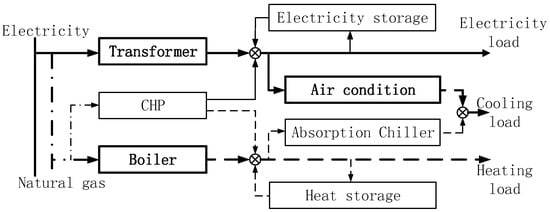
Figure 1.
Structure of the investigated energy hub.
Electricity and natural gas are delivered via the electricity and natural gas networks. These carriers are converted and stored within the hub in order to satisfy the growing requirements of the electricity, cooling, and heating loads. The thick lines represent the existing energy flow in the initial year. The thin lines represent the possible energy flow in the planning horizon.
For the energy hub illustrated in Figure 1, the supply-load balance equations can be formulated as follows:
Electricity balance equation:
Cooling balance equation:
Heating balance equation:
Infrastructure conversion equations:
As is shown in Equations (5)–(7), there are many nonlinear elements (), so in order to simplify model and reduce the computational burden, we make reasonable approximations and assumptions. The dispatch factor v is assumed to be constant. Thus, the linear energy hub is modeled in this work. Compared to non-linear energy hub model, the linear energy hub model can be solved via mathematical programming approach which is very mature nowadays.
Equations (4)–(9) demonstrate the output power of transformer, CHP, boiler, absorption chiller, and air condition to their input using efficiency coefficient, respectively.
Based on the previous equations, the flow through an energy hub are modeled by the following relation:
Input conversion matrix is the forward coupling matrix that describes the energy conversion via electricity transformer, CHP, boiler. Output coupling matrix describes how electrical storage, heat storage, absorption chiller, and air condition affect the hub output flow.
2.2. Matrix Scheme of Whole Model
The objective is the function of investment state , line flow , and curtailed loads . Equality constraints (11a–11d) include the energy hub equation, system nodal equation, energy storage equation, electricity network reconfiguration equation, respectively. Inequality constraints arise from construction logic and power limitations of elements. We define their minimal and maximal values in vector , , , as shown in Equations (11e)–(11h). Additional inequalities (11i), (11j) are given by the auxiliary parameters of electricity network reconfiguration. Finally, the problem can be mathematically expressed as follows:
Subject to:
3. Mathematical Formulation
The integrated expansion planning model is formulated as a mixed-integer quadratic programming problem (MIQP). Each element of the model is analyzed separately in order to present it explicitly.
3.1. Objective Function
The objective function of the proposed expansion planning model is to minimize the net present value of five terms that are denoted as , , , . In general, the first term () represents the cost of installing new elements and recycling the existing elements. The second term (CMnt) represents the cost of maintaining the existing and constructed elements. The third term (COpr) represents the cost of operation. The fourth term () represents the cost of interruption in electricity and natural gas systems. The objective function is given by (12):
Minimize:
We define that:
where is the state on/off (1/0) of candidate elements during each period of expansion planning horizon. For new project, this variable, which is decided to be built until its lifetime, is equal to 1 from the period , 0 otherwise. For existent element, this variable is fixed at 1 from until its lifetime, 0 otherwise. denotes the decision variables whether candidate elements is built in period . This variable, which is decided to be built in period , is equal to 1 from the period .
In general terms, the first term of (12) is the summation of seven kinds of elements’ installation costs, including CHPs, boilers, air-conditions, absorption chillers, electricity energy storages, heat energy storages, and electricity network lines, which is given by (14). The first part of this term is the investment cost of new elements. The other part represents the total benefit of recycling the existing elements. It represents the percentage of depreciation of the initial investment. is the discount rate. is the present-worth coefficient of the resources at period . For each existing elements, a higher recycle factor indicates a lower depreciation at the end of the planning horizon. is the vector of investment cost of element i in each energy hub:
where is the index for all candidate elements; and are the set of all candidate and existing elements; is the index for years.
The second term () given by (15) is the total maintenance cost of all elements including existing and new built elements in the whole planning horizon. The first part of this term is the maintenance cost of new elements. The other part represents the maintenance cost of existing elements. is the vector of maintenance cost of element i in each energy hub:
The third term () given by (16) is the operational cost of the electricity network that corresponds to the energy losses over:
It is mentioned that we assume the network does not have technical losses (gas leaks) or gas consumption due to the compressor. Therefore, we do not take operational cost of natural gas into account.
The last term () given by (17) is the total interruption cost, which is adopted as reliability index, to measure the electricity and natural gas systems’ reliability. The shedding of electricity loads, cooling loads, and heating loads are taken into account in the total expansion planning horizon:
3.2. Construction Logical Constraints
Construction logical constraints for all candidate elements in electricity and natural gas systems can be presented as (18)–(24). Once a candidate element is installed, its state in both systems will be changed to 1 for the remaining years:
3.3. Energy Hubs Constraints
Within energy hubs, electricity, cooling, and heating loads are supplied via coupling matrix Equations (25)–(27). Input energy into hubs is restricted by the elements’ characteristics and each element should be lower than the maximum level. Equation (28) imposes bounds on CHPs in each energy hub. Equations (29)–(31) ensure that the energy flow through each element is within the limits of air-conditions, absorption chillers, and boilers. For the existing elements in hubs, the maximum capacity may be changed because of installing new elements as shown in Equations (29) and (31). In order to reduce the number of intermediate variables, the output energy variable of CHPs, air-conditions, absorption chillers, and boilers are replaced by other intermediate variables. Equations (32)–(34) force the electricity, cooling, and heating loads curtailment to be no more than a certain ratio of demanded loads:
3.4. Energy Storages Constraints
Equations (35) and (40) connect the charging state of electricity storage and heat storage to their previous states of charge/discharge, input, output, and efficiencies. The capacity of storages should be located in its upper and lower operational bounds (36), (41). Charge and discharge power of electricity storage and heat storage units should be in a predetermined zone (37), (38), (42), (43). We supposed that the initial energy of storages in each season are the constant ratio of the maximum capacity (39), (44):
3.5. Electrical Distribution Network Nodal Equations and Reconfiguration Constraints
Here, Equations (45)–(48) are electrical distribution network nodal equations, which are obtained from simplified distribution power flow equations via dropping all quadratic terms and removing the voltage constraints [3]. The power flow of lines should be lower than the maximum bounds of its operation condition (49)–(50). The auxiliary variables and are continuous line orientation variables. do not equals . In fact, the and only equal zero or one, it is not necessary to force them to be discrete, and this greatly reduces the computational burden. Equation (52) states that power flow direction is from substation to other nodes. Each reconfigurable line is related to the binary variable , which is zero if the switch is open and one if closed. Equations (53)–(54) make the network reconfigurable. Equation (55) ensures the electric network is radial:
3.6. Natural Gas Distribution Network Constraints
Here, Equations (57)–(58) are natural gas distribution network nodal constraints. The limits of natural gas flow along pipelines are modeled by (59). Equation (60) states that the capacity of natural gas from upstream system should be kept at the minimum and maximum bounds of its operation condition:
3.7. Bilinear Relaxation and Whole Model
In this model, in Equations (25), (27) and (31), in Equations (49) and (50) are involved in bilinear relaxations, where and are binary variables. and are continuous variables. Therefore, we use many bilinear relaxations introduced by McCormick. Given a product between a binary variable and a continuous variable with known lower and upper bounds L and U. The relaxation is denoted by , which is equivalent to the following two set of linear constraints:
Considering the common form of Mixed Integer Quadratic Programming (MIQP) is the following:
where denotes an n-dimensional vector including integer variable and continuous variable. denotes the vector transpose of . denotes a real-valued, n-dimensional vector. denotes an n × n-dimensional real symmetric matrix. denotes an m × n-dimensional real matrix. denotes an m-dimensional real vector.
As is shown from the former part, the objective function is quadratic because Equation (16) has a quadratic term, while other terms are linear. The constraints including Equations (16)–(60) are linear because bilinear terms in Equations (25), (27), (31), (49) and (50) are changed to linear constraints via Equation (61).
Therefore, the whole model is MIQP. MIQP is a common optimization model and has a mature solution. According to the pubic standard benchmarks, maintained by Mittelmann at Arizona State University (http://plato.la.asu.edu/bench.html), MIQP also has good performance including outstanding solve times and globally optimal results just like MILP.
4. Numerical Results
In this section, the proposed expansion planning model has been tested on reconfigurable electricity and natural gas distribution systems with three and twelve energy hubs as is illustrated in Figures 3 and 4, respectively. The simple numerical example with three energy hubs aims to provide an illustration of the four objective functions, Equations (14)–(17), in Section 3. The results of systems with twelve energy hubs have been compared with six cases and verified the effectiveness of the proposed model.
4.1. Common Assumptions
The energy hubs are attached to the electricity and natural gas networks in its input and can supply electricity, cooling, and heating loads in its output. In the initial year, electricity and cooling loads are supplied only via transformer from electricity network, natural gas is supplied to feed the existing boiler for heating loads.
Figure 2 shows forecast curves for electricity, heating and cooling daily loads benchmark from an urban area in Beijing, China [43]. In order to observe the restrictions of the electricity and natural gas networks on simulation results, predicted loads are assumed to be similar for all the twelve hubs. Power factors for all the hubs are assumed to be 0.9. As is shown in this figure, 24 blocks are considered in each daily curve. The number of time blocks considered to represent yearly variations of loads is 4 (seasons) × 24 (hours) = 96 instead of 8760. This simplification is utilized here to reduce the computational burden. These discount rate is assumed to be 5% and simulations are carried out for an operation period of 5 years. Each planned candidate element is considered for installation at the beginning of each year.
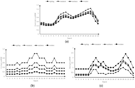
Figure 2.
Load benchmark curves during typical days of each season. (a) electricity load; (b) cooling load; (c) heating load.
The dispatch factor is assumed to be 0.5. The time interval is set to an hour. The daily electricity, cooling, and heating load has an average annual load growth rate of 5%. The average VOLL of electricity, cooling, and heating load is fixed at $30, $15, and $10/kWh, respectively. In fact, an average EVOLL of 30 $/kWh for all the electricity load shedding in these example is relatively low compared with some large commercial and industrial customers (usually is in a range of 20–100 $/kWh) [6].
4.2. Systems with Three Energy Hubs
As is shown in Figure 3, the electricity distribution network comprises three buses, four distribution lines with three reconfigurable branches, and a substation. The natural gas system is comprised of three nodes, two pipelines, and a gas supplier. It is assumed that four lines, three CHPs, three boilers, three air conditions, three absorption chillers, three electricity storages, and three heating storages are available for selection in the planning horizon. The loads are 1 times, 2 times and 3 times the benchmark from hub1 to hub3, respectively.
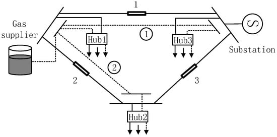
Figure 3.
Reconfigurable electricity and natural gas distribution systems with three energy hubs.
The optimization results of systems with three energy hubs are stated in Table 1, Table 2 and Table 3. As is shown in these tables, candidate lines, air conditions, and CHPs are not installed. Two of the existing boilers are replaced by the larger capacity. Absorption chillers, electricity storages, and heat storages are added to systems with the growth of loads in different years.

Table 1.
Candidate line parameters and installation year in systems with three energy hubs.
Table 2.
Candidate boiler, air condition, CHP parameters and installation year in systems with three energy hubs.
Table 3.
Candidate absorption chiller, electricity storage, heat storage parameters and installation year in systems with three energy hubs.
The objective function comprises investment cost, maintenance cost, operation cost, and interruption cost. As is shown in Figure 4, the total cost is $1.76 million. The summation of investment cost in this system is $0.203 million. The first part of this term is the installation cost of two new boilers ($0.087 million), three absorption chillers ($0.122 million), one electricity storages ($0.167 million), and heat storages ($0.025 million). The other part represents the benefit of recycling the existing two boilers ($0.032 million).
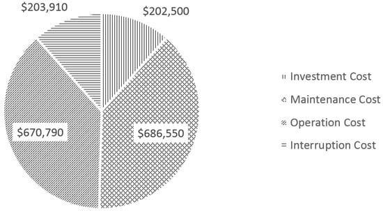
Figure 4.
Electricity and natural gas distribution systems total planning costs in systems with three energy hubs.
The maintenance cost and operation cost are relatively high than others. The total maintenance cost of all elements including existing and new built elements is $0.687 million. The maintenance cost of new and existing elements including boilers ($0.319 million), air conditions ($0.185 million), absorption chillers ($0.093 million), electricity storages ($0.032 million), and heat storages ($0.0054 million), lines ($0.605 million). The operational cost of the electricity network corresponds to the energy losses is $0.671 million.
The total interruption cost ($0.204 million) contains the cost of electricity loads ($0 million), cooling loads ($0 million), and heating loads ($0.204 million) shedding in the total expansion planning horizon. In other words, electricity loads and cooling loads are not shed due to the operational factors including energy storages and reconfiguration of electricity network.
4.3. Systems with Twelve Energy Hubs
As is shown in Figure 5, the electricity distribution network comprises twelve buses, fifty distribution lines with five reconfigurable branches, and a substation. The natural gas system is comprised of twelve nodes, eleven pipelines, and a gas supplier. It is assumed that fifteen lines, twelve CHPs, twelve boilers, twelve air conditions, twelve absorption chillers, twelve electricity storages, and twelve heating storages are available for selection in the planning horizon.
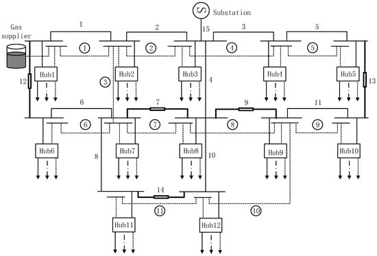
Figure 5.
Reconfigurable electricity and natural gas distribution systems with twelve energy hubs.
We assume the loads are 1 times, 2 times, 2 times, 1 times, 1 times, 1 times, 1 times, 2 times, 2 times, 1 times, 1 times and 2 times the benchmark from hub1 to hub12, respectively. There are too many input parameters in this model. Therefore, we made an Excel file which contains all the parameters and values. The full system database is available from the authors upon request.
In order to analyze the effect of different elements, CHP and absorption chiller elements, operational factor incorporation energy storage elements and reconfiguration constraints on the quality of serving loads, six different cases are defined. The differences between these cases are stated in Table 4.
Table 4.
Six cases of reconfiguration multi-energy distribution systems.
In case 0, it is assumed that different loads are served without incorporating operational factor via traditional energy networks. In other words, electricity loads are served through the electrical distribution network by transformers, cooling loads are served by air conditioner transformed only from electricity, and heating loads are supplied by boilers using natural gas. In case 1, the effect of including CHP and absorption chiller elements within the energy hub is investigated. In case 2, 3, and 4, operational factor is available by adding energy storage elements and reconfiguration constraints. In case 5, all of the different elements are included.
GUROBI is used to solve the problem in YALMIP under the MATLAB environment [44]. The algorithm has been run on a computer with an Intel Core i5 at 3.4-GHz CPU and 4 GB RAM. The calculation time for the case with reconfiguration constraints is much higher due to the various binary variables are introduced. The computational time to solve case 5 (74,174 continuous variables, 1812 integer variables, 28,800 quadratic objective terms, and 377,616 equations) is 2.8 h with epgap = 1%, when the problem is relaxed, using four threads.
(1) Case 0
The electricity and natural gas distribution systems are planned in a completely decoupled mode in this case. The growing loads are supplied via reinforcing the existing elements. The five-year planning schedules of six cases are presented in Table 5, Table 6, Table 7, Table 8, Table 9, Table 10 and Table 11. Table 5 shows the electric power system planning schedule with candidate lines. In the first year of the planning horizon, four lines including the 4th, 7th, 10th, and 15th with relatively smaller capacity are reinforced in order to meet the forecasted electricity loads and cooling loads for a total planning cost of $5.64 million. The interrupt cost is mainly from the electricity load shedding. The electricity load shedding occurs mainly during the fourth and fifth year in summer during 20 and 21 time blocks with a total EENS of 1.44 MWh and an interrupt cost of $3.25 million. In order to serve the growing cooling loads, nine air conditions are installed in energy hubs with a total planning cost of $1.1 million and an interrupt cost of $0. For the natural gas/heating systems, ten boilers are installed as is given in Table 6. The total planning cost of the decouple electricity and natural gas distribution systems to supply the increasing multiple loads at the hubs is $22.21 million in this case.
Table 5.
Candidate Line parameters and installation year in each case.
Table 6.
Candidate boiler parameters and installation year in each case.
Table 7.
Candidate air condition parameters and installation year in each case.
Table 8.
Candidate CHP parameters and installation year in each case.
Table 9.
Candidate absorption chiller parameters and installation year in each case.
Table 10.
Candidate electricity storage parameters and installation year in each case.
Table 11.
Candidate heat storage parameters and installation year in each case.
(2) Case 1
Compared to case 0, CHP and absorption chiller are considered as candidate elements in the planning process. As is shown in Figure 6, the interruption cost reduces significantly in comparison with other cases except case 5. In this case, four new absorption chillers are installed with a total investment cost of $0.5 million for serving cooling loads. The air conditions are not installed in the planning horizon. Because the efficiency of absorption chillers is much higher than for air conditioners, the cooling loads can be served from absorption chillers. Two new CHPs are scheduled in the first year, which can supply the increasing loads in hub3 and hub10. Because of the electricity, cooling and heating supply from the installed CHPs, four boilers in hub3, hub4, hub7 and hub10 is cancelled and the installation years of lines are deferred in this case. The CHPs significantly reduce the cost of interruption by $3.37 million. In addition, the maintenance and operation cost is also reduced. However, in spite of the benefit from CHPs, the investment cost of case 1 is reduced only about $0.29 million because the average cost of CHP is much higher than those of other equipment. In conclusion, the total cost of case 1 is relatively low as compared to case 0.
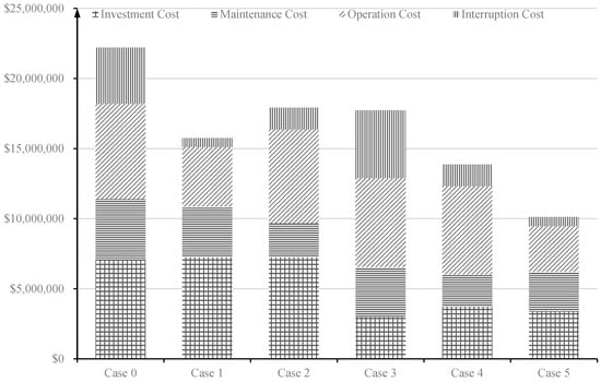
Figure 6.
Electricity and natural gas distribution system planning costs in different cases.
(3) Case 2 and case 3
We consider the part of operational factor in this case. The energy storage elements are added to case 2 in the planning schedule compared to case 0. From the view of the overall system, energy storages can smooth load fluctuation in energy hubs. Because the energy storages charge when the energy supply exceeds demand and discharge when the loads are relatively low. This feature would reduce the costs of interruption by $2.44 million compared with that in case 0. As is shown in Table 5 and Table 6, the 4th candidate line and five boilers are not installed in this case. The rest of boilers are deferred for several years, so the investment cost is slightly lower than that in case 0. Here, the operation costs are lower by $1.94 million and the total cost is $17.9 million.
The reconfiguration constraints are considered in case 3. Five branches is equipped with switches that can be activated via remote control signals. The cost of investment reduces significantly by $4.05 million compared with case 0 due to the utilization of reconfiguration, which makes maximum use of the existing lines’ capacity.
(4) Case 4
We consider all of two operational factors in this case. Both energy storage elements and reconfiguration constraints are added compared to case 0. Figure 6 shows that the investment cost of case 4 ($ 3.71 million) is lower than case 2 ($ 7.25 million), as case 4 only installs one candidate line. Even though case 4 has a higher investment cost than case 3 ($ 4.56 million), the maintenance cost ($ 2.31 million) and interruption cost ($ 1.56 million) of case 4 are lower than case 3 ($ 3.56 million, $ 4.84 million) because the maintenance cost of the boiler is higher than energy storage. In fact, the lower cost of maintenance and interruption compensates for the higher cost of investment, so that the integrated expansion planning costs less. Besides, the operation cost is relatively lower than that in case 0, case1 and case 2, because the reconfiguration and energy storage make the network operate in proper mode. The total planning cost of case 4 including the two operational factors is $13.87 million.
(5) Case 5
We consider all of the optional options in this case. Both operational factors and CHPs, absorption chillers are taken into account. As shown in Table 5, Table 6, Table 7, Table 8, Table 9, Table 10 and Table 11, none of the existing elements except the boiler in the 6th hub are replaced. Because the increasing heating and cooling loads can be served via the candidate boiler without shedding loads in the 6th hub, the electricity load can be sufficiently supplied by the reconfigurable electricity distribution network, it is not needed to install the expensive CHP. Compared to other cases, even the 15th branch is not replaced mainly due to the utilization of a high efficient CHPs and CHPs make electricity system and natural gas system support each other, and the electrical input power decreases significantly during peak hours. The four new absorption chillers reduce electricity demand and relieve the pressure on the electricity distribution network. The electricity storages are installed in the last two years of the planning horizon because the electricity loads shedding always occur at this time. The heating storages are nearly installed in the first and second year mainly due to the unit investment cost of heating storage is relatively low.
Case 6 has the lowest operation cost ($ 0.66 million) own to the CHPs and operational factors. The investment, maintenance, and operation cost are relatively low compared with other cases. Therefore, case 6 has the lowest total cost ($ 10.12 million) and less than half of case 0.
5. Conclusions and Future Work
With increasing worldwide low carbon concerns, natural gas is believed to be a relatively clean fuel compared to other forms of resources. The availability of natural gas for serving electricity loads can significantly influence the reliability of electricity distribution network. The operational factors including reconfiguration and energy storages in multi-stage expansion co-planning have profound impacts on energy load fluctuation, consequently affecting the overall cost. In this paper, a novel method is presented to model and formulate the optimal design of reconfiguration electricity and natural gas distribution systems. The model can analyze interactions between electricity and natural gas systems serving electricity, cooling, and heating loads.
The numerical results show the usefulness of CHPs and absorption chillers, and operational factors including energy storages and reconfiguration. The proposed approach reduces the expansion cost of integrated distribution systems, as compared to the decoupled approach where electricity and natural gas networks are planned as separate systems. The reasons why cost reductions are achieved can be summarized as follows:
- CHPs make electricity system and natural gas system couples. They can mutually support each other when necessary.
- Cooling loads can be supplied via both air conditioners and absorption chillers. The new absorption chillers can make full use of produced heating energy and reduce the demand for electricity. This relieves the pressure on the electricity distribution network to some extent.
- Energy storages smooth load fluctuations in energy hubs. They can defer or avoid the installation of new elements.
- The reconfigurable characteristics of the electricity distribution network can make full use of the existing lines’ capacity.
The optimization problem is modeled as a MIQP problem, which can be solved via fast and accurate commercial solvers. The proposed model can help electricity and natural gas distribution systems planners determine the most economical elements that should be purchased and installed in order to meet energy demands (electricity, cooling, and heating). Utilizing the proposed model for both systems not only increases load reliability, but also decreases the cost of serving energy to customers at the same time. By simulating the integrated operational behavior of the two systems in the planning horizon, our model can strategically give the optimum planning recommendations to both sectors simultaneously.
The formulation presented in this paper is focused on simplified gas network equations without considering gas flow equations. In the future work should be carried out to obtain a more detailed natural gas network model by including compressors and pipelines. Natural gas network equations are diverse in different gas pressure level. So we should model natural gas system in a more accurate way. On the other hand, with increasingly penetration of some distributed generation, which can couple electricity and natural gas networks, future research is also needed to take the uncertainty into account in a market environment.
Author Contributions
Xianzheng Zhou proposed the research, wrote and revised the paper. Chuangxin Guo, supervised the research. Yifei Wang and Wanqi Li assisted the research.
Conflicts of Interest
The authors declare no conflict of interest.
Nomenclature
| Indices | |
| Index for component in energy hubs | |
| Index for years | |
| Index for hours | |
| Index for seasons | |
| Index for natural gas suppliers | |
| Index for natural gas pipelines | |
| Sets | |
| Set of all candidate elements | |
| Set of candidate CHPs | |
| Set of candidate boilers | |
| Set of candidate air conditions | |
| Set of candidate absorption Chillers | |
| Set of candidate electricity storages | |
| Set of candidate heat storages | |
| Set of candidate distribution lines | |
| Set of all existing elements | |
| Set of existing boilers | |
| Set of existing air conditions | |
| Set of existing distribution lines | |
| Set of electricity lines | |
| Set of electricity lines with switches | |
| Set of electricity lines without switches | |
| Set of electricity buses | |
| Set of buses which are substations | |
| Set of buses which are not substations | |
| Set of natural gas buses | |
| Set of natural gas buses which are gas suppliers | |
| Set of natural gas buses which are not gas suppliers | |
| Set of natural gas pipelines. | |
| Set of lines connect with bus and gas supplier | |
| Constants | |
| Number of years in planning horizon | |
| Discount rate | |
| Voltage amplitude at each electricity buses | |
| Time interval | |
| Electrical/Cooling/Heating loads in hub output | |
| Dispatch factor | |
| Efficiency of transformer | |
| Efficiency of gas to electricity/heat conversion in a combined heat and power (CHP) | |
| Efficiency of gas to heat conversion in boiler | |
| , , , , , , | Investment cost of CHPs/boilers/air conditions/absorption chillers/electricity storages/heat storages/distribution lines |
| Efficiency of heat to cool conversion in absorption chiller | |
| Maximum capacity of electricity/heat storage | |
| Maximum factor of electricity/heat storage’s maximum capacity. | |
| Minimum factor of electricity/heat storage’s maximum capacity. | |
| Maximum output electric/heat power of electricity/heat storage. | |
| Initial energy level of electricity/heat storage. | |
| Initial factor of electricity/heat storage’s maximum capacity | |
| Maximum/Minimum capacity of gas suppliers | |
| Maximum/Minimum flow of in natural gas pipeline. | |
| , , | Value of unit lost electricity/cooling/heating load. |
| Resistance of the line from bus to | |
| Salvage factor for boilers/air conditions/lines | |
| Efficiency of electricity to cool conversion in air condition | |
| , , , , , , | Maintenance cost of CHPs/boilers/air conditions/absorption chillers/electricity storages/heat storages/distribution lines |
| Maximum capacity of CHPs and absorption | |
| Maximum capacity of existing and candidate air-conditions | |
| Maximum capacity of existing and candidate boilers | |
| Variables | |
| Total investment cost | |
| Total maintenance cost | |
| Total operation cost | |
| Total interruption cost | |
| Investment state of candidate elements | |
| Investment state of CHPs | |
| Investment state of boilers | |
| Investment state of air conditions | |
| Investment state of absorption Chillers | |
| Investment state of electricity storages | |
| Investment state of heat storages. | |
| Investment state of distribution lines | |
| Electricity active power input within a hub | |
| Electricity active power output from a substation | |
| Real power flow from bus to | |
| Electricity reactive power input within a hub | |
| Electricity reactive power output from a substation | |
| Heat power input within a hub | |
| Natural gas pipeline flow | |
| Output/Input electric power of electricity storage | |
| Input cooling power of an air condition | |
| Output/Input electric power of heat storage | |
| Input cooling power of an absorption chiller | |
| Energy level of electricity/heat storage | |
| Output electric/heat power of electricity/heat storage. | |
| Input electric/heat power of electricity/heat storage | |
| Discrete switch variable. | |
| Continuous line orientation variable | |
| Gas delivery quantity of supplier | |
| Curtailed electricity/cooling/heating load | |
References
- Mancarella, P. MES (multi-energy systems): An overview of concepts and evaluation models. Energy 2014, 65, 1–7. [Google Scholar] [CrossRef]
- Krause, T.; Andersson, G.; Frohlich, K.; Vaccaro, A. Multiple-energy carriers: modeling of production, delivery, and consumption. Proc. IEEE 2011, 99, 15–27. [Google Scholar] [CrossRef]
- Taylor, J.A.; Hover, F.S. Convex models of distribution system reconfiguration. IEEE Trans. Power Syst. 2012, 27, 1407–1413. [Google Scholar] [CrossRef]
- Salimi, M.; Ghasemi, H.; Adelpour, M.; Vaez-Zadeh, S. Optimal planning of energy hubs in interconnected energy systems: A case study for natural gas and electricity. IET Gener. Transm. Distrib. 2015, 9, 695–707. [Google Scholar] [CrossRef]
- Geidl, M.; Andersson, G. Optimal coupling of energy infrastructures. In Proceedings of the 2007 IEEE Lausanne Power Tech, Lausanne, Switzerland, 1–5 July 2007; pp. 1398–1403.
- Saldarriaga, C.A.; Hincapié, R.A.; Salazar, H. A holistic approach for planning natural gas and electricity distribution networks. IEEE Trans. Power Syst. 2013, 28, 4052–4063. [Google Scholar] [CrossRef]
- Nazar, M.S.; Haghifam, M.R. Multiobjective electric distribution system expansion planning using hybrid energy hub concept. Electric. Power Syst. Res. 2009, 79, 899–911. [Google Scholar] [CrossRef]
- Unsihuay-Vila, C.; Marangon-Lima, J.W.; de Souza, A.; Perez-Arriaga, I.J.; Balestrassi, P.P. A model to long-term, multiarea, multistage, and integrated expansion planning of electricity and natural gas systems. IEEE Trans. Power Syst. 2010, 25, 1154–1168. [Google Scholar] [CrossRef]
- Barati, F.; Seifi, H.; Sepasian, M.S.; Nateghi, A.; Shafie-khah, M.; Catalão, J.P. Multi-period integrated framework of generation, transmission, and natural gas grid expansion planning for large-scale systems. IEEE Trans. Power Syst. 2015, 30, 2527–2537. [Google Scholar] [CrossRef]
- Qui, J.; Yang, H.; Dong, Z.Y.; Zhao, J.; Meng, K.; Luo, F.J.; Wong, K.P. A Linear Programming Approach to Expansion Co-Planning in Gas and Electricity Markets. IEEE Trans. Power Syst. 2015, 31, 3594–3606. [Google Scholar]
- Qiu, J.; Dong, Z.Y.; Zhao, J.H.; Meng, K.; Zheng, Y.; Hill, D.J. Low carbon oriented expansion planning of integrated gas and power systems. IEEE Trans. Power Syst. 2015, 30, 1035–1046. [Google Scholar] [CrossRef]
- Zhang, X.; Karady, G.G.; Ariaratnam, S.T. Optimal allocation of CHP-based distributed generation on urban energy distribution networks. IEEE Trans. Sustain. Energy 2014, 5, 246–253. [Google Scholar] [CrossRef]
- Saldarriaga, C.A.; Salazar, H. Security of the Colombian energy supply: the need for liquefied natural gas regasification terminals for power and natural gas sectors. Energy 2016, 100, 349–362. [Google Scholar] [CrossRef]
- Saldarriaga, C.A.; Hincapie, R.A.; Salazar, H. An integrated expansion planning model of electric and natural gas distribution systems considering demand uncertainty. In Proceedings of the 2015 IEEE Power & Energy Society General Meeting, Denver, CO, USA, 26–30 July 2015; pp. 1–5.
- Saldarriaga, C.A.; Hincapie, R.A.; Salazar, H. A Multi-Objective Analysis for Planning Electric and Natural Gas Distribution Networks. In Proceedings of the 2015 IEEE PES Innovative Smart Grid Technologies Latin America (ISGT LATAM), Montevideo, Uruguay, 5–7 October 2015; pp. 456–461.
- Rieder, A.; Christidis, A.; Tsatsaronis, G. Multi criteria dynamic design optimization of a small scale distributed energy system. Energy 2014, 74, 230–239. [Google Scholar] [CrossRef]
- Weber, C.; Shah, N. Optimization based design of a district energy system for an eco-town in the United Kingdom. Energy 2011, 36, 1292–1308. [Google Scholar] [CrossRef]
- Bracco, S.; Dentici, G.; Siri, S. Economic and environmental optimization model for the design and the operation of a combined heat and power distributed generation system in an urban area. Energy 2013, 55, 1001–1014. [Google Scholar] [CrossRef]
- Koeppel, G.; Korpås, M. Improving the network infeed accuracy of non-dispatchable generators with energy storage devices. Electr. Power Syst. Res. 2008, 78, 2024–2036. [Google Scholar] [CrossRef]
- Moeini-Aghtaie, M.; Abbaspour, A.; Fotuhi-Firuzabad, M.; Hajipour, E. A decomposed solution to multiple-energy carriers optimal power flow. IEEE Trans. Power Syst. 2014, 29, 707–716. [Google Scholar] [CrossRef]
- Koeppel, G.; Andersson, G. Reliability modeling of multi-carrier energy systems. Energy 2009, 34, 235–244. [Google Scholar] [CrossRef]
- Haghifam, M.R.; Manbachi, M. Reliability and availability modelling of combined heat and power (CHP) systems. Int. J. Electr. Power Energy Syst. 2011, 33, 385–393. [Google Scholar] [CrossRef]
- Arnold, M.; Negenborn, R.R.; Andersson, G.; De Schutter, B. Distributed control applied to combined electricity and natural gas infrastructures. In Proceedings of the First International Conference on Infrastructure Systems: Building Networks for a Brighter Future (INFRA 2008), Rotterdam, The Netherlands, 10–12 November 2008.
- Arnold, M.; Negenborn, R.R.; Andersson, G.; De Schutter, B. Model-based predictive control applied to multi-carrier energy systems. In Proceedings of the 2009 IEEE Power & Energy Society General Meeting, Calgary, AB, Canada, 26–30 July 2009; pp. 1–8.
- Schulze, M.; Del Granado, P.C. Optimization modeling in energy storage applied to a multi-carrier system. In Proceedings of the 2010 IEEE Power & Energy Society General Meeting, Minneapolis, MN, USA, 25–29 July 2010; pp. 1–7.
- Kienzle, F.; Trutnevyte, E.; Andersson, G. Comprehensive performance and incertitude analysis of multi-energy portfolios. In Proceedings of the 2009 IEEE Bucharest PowerTech, Bucharest, Romania, 28 June–2 July 2009; pp. 1–6.
- Galus, M.D.; Andersson, G. Power system considerations of plug-in hybrid electric vehicles based on a multi energy carrier model. In Proceedings of the 2009 IEEE Power & Energy Society General Meeting, Calgary, AB, Canada, 26–30 July 2009; pp. 1–8.
- Kienzle, F.; Andersson, G. Efficient multi-energy generation portfolios for the future. In Proceedings of the 4th Annual Carnegie Mellon Conference on the Electricity Industry, Pittsburgh, PA, USA, 10–11 March 2008; pp. 1–18.
- Geidl, M.; Andersson, G. Operational and structural optimization of multi-carrier energy systems. Eur. Trans. Electr. Power 2006, 16, 463–477. [Google Scholar] [CrossRef]
- Sheikhi, A.; Ranjbar, A.M.; Oraee, H. Financial analysis and optimal size and operation for a multicarrier energy system. Energy Build. 2012, 48, 71–78. [Google Scholar] [CrossRef]
- Barbieri, E.S.; Dai, Y.J.; Morini, M.; Pinelli, M.; Spina, P.R.; Sun, P.; Wang, R.Z. Optimal sizing of a multi-source energy plant for power heat and cooling generation. Appl. Therm. Eng. 2014, 71, 736–750. [Google Scholar] [CrossRef]
- Shahmohammadi, A.; Moradi-Dalvand, M.; Ghasemi, H.; Ghazizadeh, M.S. Optimal design of multicarrier energy systems considering reliability constraints. IEEE Trans. Power Deliv. 2015, 30, 878–886. [Google Scholar] [CrossRef]
- Fabrizio, E.; Corrado, V.; Filippi, M. A model to design and optimize multi-energy systems in buildings at the design concept stage. Renew. Energy 2010, 35, 644–655. [Google Scholar] [CrossRef]
- Sharif, A.; Almansoori, A.; Fowler, M.; Elkamel, A.; Alrafea, K. Design of an energy hub based on natural gas and renewable energy sources. Int. J. Energy Res. 2014, 38, 363–373. [Google Scholar] [CrossRef]
- Zhang, X.; Shahidehpour, M.; Alabdulwahab, A.; Abusorrah, A. Optimal expansion planning of energy hub with multiple energy infrastructures. IEEE Trans. Smart Grid 2015, 6, 2302–2311. [Google Scholar] [CrossRef]
- Maroufmashat, A.; Elkamel, A.; Fowler, M.; Sattari, S.; Roshandel, R.; Hajimiragha, A.; Walker, S.; Entchev, E. Modeling and optimization of a network of energy hubs to improve economic and emission considerations. Energy 2015, 93, 2546–2558. [Google Scholar] [CrossRef]
- Maroufmashat, A.; Sattari, S.; Roshandel, R.; Fowler, M.; Elkamel, A. Multi-objective Optimization for Design and Operation of Distributed Energy Systems through the Multi-energy Hub Network Approach. Ind. Eng. Chem. Res. 2016, 55, 8950–8966. [Google Scholar] [CrossRef]
- Maroufmashat, A.; Fowler, M.; Khavas, S.S.; Elkamel, A.; Roshandel, R.; Hajimiragha, A. Mixed integer linear programing based approach for optimal planning and operation of a smart urban energy network to support the hydrogen economy. Int. J. Hydrog. Energy 2016, 41, 7700–7716. [Google Scholar] [CrossRef]
- Mehleria, E.D.; Sarimveis, H.; Markatos, N.C.; Papageorgiou, L.G. Optimal design and operation of distributed energy systems: Application to Greek residential sector. Renew. Energy 2013, 51, 331–342. [Google Scholar] [CrossRef]
- Pazouki, S.; Mahmoud, R.H. Optimal planning and scheduling of energy hub in presence of wind, storage and demand response under uncertainty. Int. J. Electr. Power Energy Syst. 2016, 80, 219–239. [Google Scholar] [CrossRef]
- Xu, X.; Hou, K.; Jia, H. A reliability assessment approach for the urban energy system and its application in energy hub planning. In Proceedings of the 2015 IEEE Power & Energy Society General Meeting, Denver, CO, USA, 26–30 July 2015; pp. 1–8.
- Zhang, X.; Che, L.; Shahidehpour, M.; Alabdulwahab, A.S.; Abusorrah, A. Reliability based optimal planning of electricity and natural gas interconnections for multiple energy hubs. IEEE Trans. Smart Grid 2015, 99, 1–10. [Google Scholar] [CrossRef]
- Yang, Y.; Pei, W.; Qu, H.; Xiao, H.; Qi, Z. A planning method of distributed combined heat and power generator based on generalized benders decomposition. Autom. Electr. Power Syst. 2014, 38, 27–33. (In Chinese) [Google Scholar]
- Gurobi Optimization Inc. Gurobi Optimizer Reference Manual; Gurobi Optimization: Houston, TX, USA, 2014. [Google Scholar]
© 2017 by the authors; licensee MDPI, Basel, Switzerland. This article is an open access article distributed under the terms and conditions of the Creative Commons Attribution (CC-BY) license (http://creativecommons.org/licenses/by/4.0/).