Article

A Mathematical Formulation of the Valuation of Ether and Ether Derivatives as a Function of Investor Sentiment and Price Jumps

by
Rebecca Abraham
1,* and
Hani El-Chaarani
2
1
Huizenga College of Business-SBE, Nova Southeastern University, 3301 College Avenue, Fort Lauderdale, FL 33314, USA
2
Department of Finance, College of Business, Tripoli Campus, Beirut Arab University, Riad El Solh, P.O. Box 11-50-20, Beirut 11072809, Lebanon
*
Author to whom correspondence should be addressed.
J. Risk Financial Manag. 2022, 15(12), 591; https://doi.org/10.3390/jrfm15120591
Submission received: 28 October 2022 / Revised: 1 December 2022 / Accepted: 2 December 2022 / Published: 8 December 2022
(This article belongs to the Special Issue FinTech, Blockchain and Cryptocurrencies)

Abstract

:
The purpose of this study was to create quantitative models to value ether, ether futures, and ether options based upon the ability of cryptocurrencies to transform existing intermediary-verified payments to non-intermediary-based currency transfers, the ability of ether as a late mover to displace bitcoin as the first mover, and the valuation of ether in the context of investor irrationality models. The risk-averse investor’s utility function is a combination of expectations of the performance of ether, expectations of cryptocurrencies’ transformative power, and expectations of ether superseding bitcoin. The moderate risk-taker’s utility function is an alt-Weibull distribution, along with a gamma distribution. Risk-takers have a utility function in the form of a Bessel function. Ether price functions consist of a Levy jump process. Ether futures are valued as the combination of current spot prices along with term prices. The value of spot prices is the product of a spot premium and a lognormal distribution of spot prices. The value of term prices is equal to the product of a term premium, and the Levy jump process of price fluctuations during the delivery period. For ether options, a less risky ether option portfolio offsets ether’s risk by a fixed-income trading strategy.

1. Introduction

The popular press has reported a surge in bitcoin prices, with prices in 2017 alone rising 17-fold (Lam and Wee 2017), up from a valuation of less than a penny in 2009 (Wood 2017). In recent years, prices have declined sharply. Bitcoin peaked at more than $68,000 in 2021, falling to less than $18,000 in November, 2022 (Levy and Sigalos 2022). As the currency of the blockchain, bitcoin prices may be attributed to rational expectations of the blockchain’s projected capabilities (Abraham 2018). Ether is a rival cryptocurrency generated by the Ethereum platform. The blockchain is a public ledger that permits the single recording of transactions in blocks, with blocks created and maintained by network participants. The financial benefits of the blockchain are in cross-border money transfers and in microfinancing. The transfer of bitcoin with oversight by network participants, rather than intermediaries, results in currency transfers with no central bank intervention. This permits the transfer of large amounts of funds, as may occur in healthcare or insurance. At the opposing extreme, very small transfers of $1.00 may occur, permitting the unbanked population to participate in financial services and microfinance very small businesses. The uncertainty of the transformative platform may have contributed to price speculation.
A key research question is the valuation of bitcoin and other cryptocurrencies. As bitcoin was not issued by a government, but has fixed supply, fiat money valuation models with unlimited supply are untenable. Ether, on the other hand, does not have fixed supply. However, like other cryptocurrencies, it does not generate a stream of dividends, so dividend discount models cannot be used for their valuation. In essence, high volatility, and fluctuating prices, suggest the inapplicability of traditional option valuation models.
An early valuation model for bitcoin suggested that the marginal cost model explained the value of bitcoin (Hayes 2017). Hayes (2017) viewed bitcoin as having intrinsic value because bitcoin mining consumes electric power, which generates a cost for miners. The value of bitcoin becomes an embedded cost of production. Nasir et al. (2019) and Burgrraf et al. (2020) considered investor sentiment to be the primary determinant of bitcoin prices. They tested this proposition empirically, finding that it was true, observing that investors reallocated their bitcoin holdings in keeping with changes in market sentiment. We support the notion of investor sentiment driving cryptocurrency prices. Accordingly, we created a mathematical model to value ether, a cryptocurrency that has had virtually no valuation models. We add additional variables to describe price movements independent of investor sentiment, as we are cognizant of bitcoin’s prices being discontinuous, also termed jump discontinuities.
The purpose of this paper is to describe the valuation of ether, ether futures, and ether options. First, we theorize on (1) the ability of cryptocurrencies to transform existing intermediary-verified payments to non-intermediary-based currency transfers, (2) the ability of ether as a late mover to displace bitcoin as the first mover into the cryptocurrency market, based on the strategic management theory of first-mover advantage, and (3) the valuation of ether in the context of theories of investor irrationality, such as the Miller (1977) model of investor optimism. Next, we describe our formulation for ether futures. Finally, we value put and call options on ether.
First-mover advantage theory (Leiberman and Montgomery 1988) posits that a proprietary learning curve creates barriers to entry. Distributed ledger technology creates a new business model with a network of protocols and tokens (Oxford Analytics Daily Brief Services 2018), creating a trade secret. Yet, bitcoin’s first-mover advantages dissipated rapidly as workforce mobility, research publications, and informal communications diffused first-mover knowledge to other firms (Spence 1984). As a late mover, ether has had to exploit technological limitations in the existing bitcoin-based network by providing a generalizable proof-of-work by the Ehash algorithm compared to bitcoin’s specialized ASCIs in mining, suitability for building blockchain products, energy efficiency, cost savings, and superior speed (Malwa 2018). Ether may be able to compete effectively with bitcoin, as did the sample of 793 U.S. and Canadian firms in Yip’s (1982) study who showed the ability of late movers to circumvent barriers to entry to markets with established incumbents. Keynes (1936) set forth that speculation occurs when an asset is purchased with the expectation of earning short-term gains at a price higher than the future value of dividends. Harrison and Kreps (1978) and Shleifer and Vishny (1977) conjectured that the very act of certain traders holding the asset sends positive signals about its future value to their peers, who would be stimulated to purchase at prices in excess of its current valuation. Rational arbitrageurs observe the overpricing as a signal to short-sell. However, the high interest rates for borrowing stock to be short-sold prevent short-selling. Using the breadth of mutual fund ownership as a proxy for the number of traders, Chen et al. (2002) found that the small number of optimists were represented by the narrowest breadth of mutual fund ownership, which underperformed the highest decile of pessimists by 6.38% in returns.
Ether futures consist of a binding contract to purchase ether at the futures price, with settlement occurring at the end of the delivery period, three to six months later. This investment is currently under regulatory review by the Commodity Futures Trading Commission (Bain 2018). The futures price is a combination of the spot price and the term price due to price fluctuations during the delivery period. Fama (1984) viewed a commodity’s value as being based upon current ether spot prices. Empirically, he found that the forward premium diverged significantly from the spot price for 11 currencies, suggesting that ether’s value during the delivery period may be different from its spot price. Gorton et al. (2012) analyzed 31 commodity futures to find increased dependence of commodity values on the delivery period.
Naked call and put options on ether provide insurance. If there is a call option on ether, a buyer may exercise the option, obtain ether at low prices, and sell at high prices, thereby earning substantial gains. If there is a put option on ether, option exercise permits sale at high prices with repurchase at low prices, yielding gains. Easley et al. (1998) suggested purchasing a call, purchasing the underlying stock, and selling a put for rising asset prices. Selling a call, purchasing a put, and selling the underlying asset are advised for falling asset prices. Cox et al.’s (1981) H model purchased put options on futures, along with interest-bearing bonds. We contend that neither of these strategies could be employed for ether’s highly risky and constantly fluctuating prices. Therefore, our valuation models are considerably different from existing valuation models.

2. Review of Literature

The Blockchain As A Transformative Asset. The blockchain’s ability to eliminate intermediaries involved in payment verification, transaction processing, and record-keeping surpasses cross-border payments to include land titling, passport, will, and patent replacement is foundationally transformative (Ishanti and Lakhani 2017). Ishanti and Lakhani (2017) compare the development of a cryptocurrency foundation to the three-decade-long cycle that resulted in the Internet. The 1970s oversaw the conversion of telecommunications architecture based on circuit-switching to digitizing information into small packets. Then, localized private networks were created to replace existing local network technologies. The Web, with new businesses providing the hardware and software to connect to it, emerged in the 1990s. This was followed by Internet services that scaled at minimal cost, expanding news availability, books for sale, and airline ticket choices, etc. Transformative applications ultimately emerged with distributed networks of users through online auctions, music streaming, video streaming, and web searches. Likewise, blockchain-based smart contracts may take decades to become mainstream entities.
Price Optimism. Miller (1977) theorized that investors have heterogeneous expectations of security returns. Increasing heterogeneity of expectations results in an increase in both optimists and pessimists. Pessimists refrain from trading while the growing proportion of optimists bids up security prices. Mian and Sankaraguruswamy (2012) and Kent and Hirshleifer (2015) perceived investor optimism as the product of overconfidence in personal capabilities for predicting security prices with positive returns providing self-affirmation, while negative returns were dismissed as chance.
The inability of rational arbitrageurs to contain irrational exuberance was observed in the technology bubble of 2000–2002. Brunnermeir and Nagel (2004) found that uninformed traders chose to maintain holdings of depreciating technology stock, due to the preponderance of expectations of positive returns during the next period. Informed traders purchased in sufficiently large volume at trade prices substantially above the bid-ask midpoint, driving prices upwards. Upon prices reaching a local maximum, they sold en masse at a bid price below the bid-ask midpoint, signaling the forthcoming price decline (Cespa and Vives 2012; Park and Sabourian 2011).
Research on Investor Sentiment and Cryptocurrencies. The uniqueness of investor sentiment in cryptocurrencies has resulted in unique measures of cryptocurrencies. Kristoufek (2013) measured investor sentiment in terms of the volume of Google search queries and Wikipedia search volume. Word-of-mouth feedback loops measured investor sentiment preceding price bubbles (Garcia et al. 2014). Garcia and Schweitzer (2015) created a trading algorithm, generating significantly high profits, using positive and negative signals from Twitter posts as the measure of investor sentiment. In a contemporary examination, Google search volume was used as a proxy for investor sentiment in the measurement of cryptocurrency returns and volatility (Eom et al. 2019).
Research in Commodity Futures. Carry trade strategies borrow in low-interest rate funding currencies, lending in high-interest rate investment currencies. Yet, uncovered interest parity eliminates gains in the appreciation of the funding currency or depreciation of the investment currency. Burnside et al. (2006) suggested hedging appreciation risk with a call option and hedging depreciation risk with a put option. For example, if borrowing occurs in the yen and the yen appreciates, the investor loses upon repaying the yen loan. To hedge, the investor purchases a call option on yen, making a gain upon yen appreciation. The gain on the call option partly offsets the loss on repayment in appreciated currency. Likewise, if lending occurs in the Mexican peso and the peso depreciates, the investor will pay an excessive amount to repay the loan; yet will gain on a put option on the peso.
Research in Currency Options. Given that ether is a currency, it is appropriate to review the literature on currency options. The seminal Black–Scholes call option pricing formula, which valued call options on stock, could not be directly applied to the valuation of foreign currencies as it failed to account for the interest rate that influences currency values. Abraham (2018) overcame this shortcoming by assuming that the relevant interest rate on a foreign currency option was the rate on a riskless domestic bond. In addition, the interest rate on a riskless bond was shown depend on the prices of currencies, with small increases in value or large increases in value (Abraham 2018). These small and large increases in value are termed price jumps.

3. Findings and Analysis

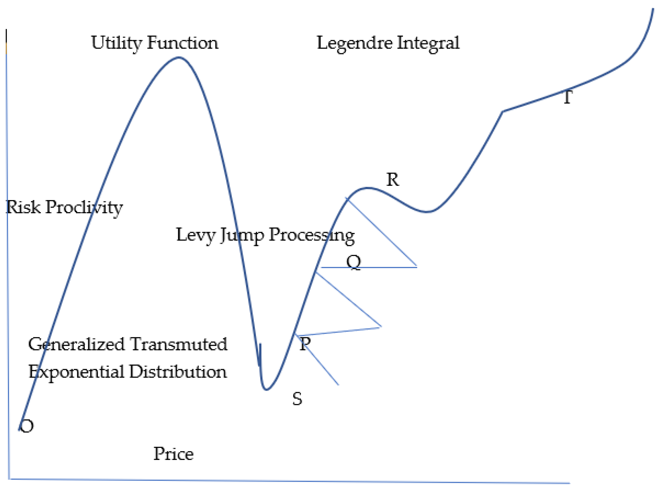
3.1. Valuation of Ether by the Risk-Averse Investor

The risk-averse investor maximizes utility, which is a combination of (1) satisfaction with the general performance of ether investments, represented by a generalized transmuted exponential distribution, (2) expectations of the transformative power of cryptocurrencies, represented by a gamma distribution, (3) a Legendre integral of expectations of ether superseding bitcoin, and (4) a gradient vector to reduce leptokurtic tail risk.
1. Investor sentiment expecting ether prices to continue to grow exponentially.
Investor sentiment is indicated by the following expression,
( 1 + λ ) [ 1 exp ( α   γ   x ) ] ] λ [ 1 exp ( α   γ   x ) 2   α > 0 ,   | λ 1 | ,
where
  • λ = the exponents of the exponential distribution, or the amount by which ether prices increase,
  • α, γ = constants in the generalized transmuted exponential distribution,
  • x = the price of ether in the generalized transmuted exponential distribution.
2. Investor expectations of the transformative power of cryptocurrencies is represented by a gamma distribution,
( k 1 ) ln x i x i / θ N k ln ( θ ) N ln ( Γ ( k ) ) ,
where
  • x1 = price of ether,
  • k = constant in the gamma distribution,
  • θ = step function of the gamma distribution,
3. Investor expectations of the likelihood of ether prices surpassing bitcoin.
( 1 z 2 ) d 2 w / d z 2 2 z d w / d z
where
  • x = price of ether,
  • d = constant,
  • w = expectation of ether superseding bitcoin in price.
  • z = z is a real number in the interval −1 ≤ x ≤ 1.
4. A gradient vector to reduce tail risk.
Cryptocurrency distributions have high risk, found in large end points (tails) of a flat leptokurtic distribution of prices. There are few observations in the center of the distribution, with a large number of observations in the tails. Therefore, v, the gradient vector, is included in the expression below, to reduce tail risk.
v ( v + 1 ) μ 2 / ( 1 e 2 ) ] w
where
  • v = gradient vector in a leptokurtic distribution of ether prices,
  • X = price of ether in the leptokurtic distribution,
  • μ 2 = mean of a leptokurtic distribution,
  • w = investor expectations of tail risk,
  • e 2 = variance of ether prices in the tails, or actual tail risk.

Objective Function and Constraints

The objective function and constraints of the model to value ether by the risk-averseinvestor is as follows (variables have been defined above):
M a x ( 1 + λ ) [ 1 exp ( α   γ   x ) ] ] λ [ 1 exp ( α   γ   x ) 2   α > 0 ,   | λ 1 | + ( k 1 ) ln x i x i / θ N k ln ( θ ) N ln ( Γ ( k ) ) + ( 1 z 2 ) d 2 w / d z 2 2 z d w / d z + [ v ( v + 1 ) μ 2 / ( 1 e 2 ) ] w
This objective function is subject to the following constraints:
x 1 + x 2 + x 3 + x 4 > y 1 + y 2 + y 3 + y 4
The first constraint in Equation (2) requires that x1x4, the attributes of ether supersede the attributes of bitcoin, y1y4, in achieving utility, where
x1x4 = the attributes of ether, including adaptability of the Ehash algorithm in building blockchain products (x1), energy efficiency (x2), cost savings (x3), and superior speed (x4).
y1yn = the attributes of bitcoin, including specialized ASCI mining (y1), an established supplier network (y2), name recognition (y3), and market share (y4).
γ t + B t + | x | 1 , s { 0 , t } x J x ( d s , d x ) + | x | 1 , s { 0 , t } x J x d s d x + l i m ε [ 0 , t ] x { J x ( d s , d x ) v ( d x , d s ) H
The second constraint, in Equation (3), describes the price distribution of ether. Ether prices do not rise continuously. They break into sudden upward movements called jumps, which are not related to existing prices. We model jumps as a Levy process, in the form of a Poisson process of jump discontinuities in ether prices, where γt = drift, Bt = Brownian motion, xJx ds x < 1, for small jumps, and xJx ds dx x > 1 for large jumps.
[ ( 0.5 ρ 1 s 2 ) ( 1 / 6 ρ 3 s 3 ) ] [ ρ 2 3 ρ ( m e a n ) 2 + ρ ( m e a n ) ] s 4 / 24 ρ 5 α [ s 1 / 6 ρ 2 s 3 + { ρ ( m e a n ) / 8 ρ 4 } s s s s = H
The third constraint in Equation (4) is unique to the risk-averse investor. This investor dislikes risk to the extent that he or she will demand compensation for accepting the risk inherent in ether. The price distribution of ether must indicate the level of risk-aversion of the investor so that the assumption of risk is only accepted with compensation in the form of a liquid, fixed-income security, with payoff H. Investing in ether is aberrant for a risk-averse investor. The left side of Equation (4) shows Schot’s (1978) expression for aberrant behavior. Risk-averse investors will demand compensation in the form of H, the value of this fixed-income security. The symbols used in Equation (4) are described below.
  • s = arc length of the secant line,
  • ρ = radius of curvature of the line of aberrancy at the point of tangency,
  • xt = expectation of ether valuation,
  • yt = risk aversion towards ether investment (Schot 1978).
Figure 1 graphically depicts the optimal value of ether obtained upon solution of Equations (1)–(4). The solution procedure is contained in Appendix A.
OS is the utility function for a risk-averse investor. TY is the Legendre integral of ether superseding bitcoin. Points P, Q, and R represent the satisfaction of utility with ether prices specified by a Levy Jump Process.

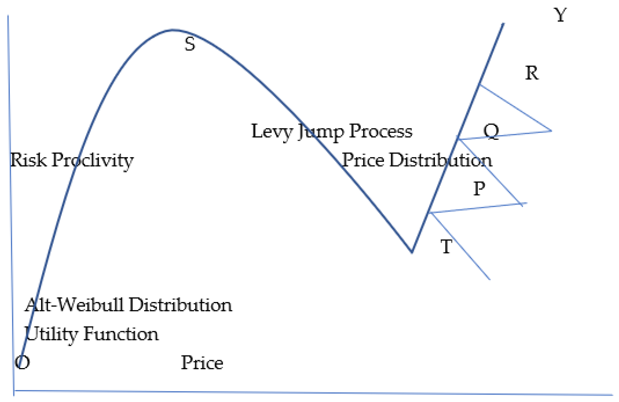
3.2. Valuation of Ether by the Moderate Risk-Taker

The moderate risk-taker is willing to tolerate some risk, though not excessive risk.
The moderate risk-taker selects a portfolio mix of 20% large-cap stocks, 8% small-cap stocks, 20% overseas developed nations, 4% emerging markets, and 40% diversified fixed-income investments.
The moderate risk-taker has the same objective function of accepting investments whose returns must justify the risk taken, as the risk-averse investor. Therefore Equation (9) is identical to Equation (1). Yet, the moderate risk-taker differs from the risk-averse investor, in that he or she is willing to tolerate more risk. The mathematical representation of willingness to tolerate some risk is the Arrow–Pratt coefficient of risk-aversion, −u″(c)/u′(c), constant, or the reduction in risk aversion with risky ether investments; it increases at a stable constant rate, suggesting a relatively flat utility function with slight positive slope.
Another representation of the moderate risk-taker’s utility function is (1) an alt-Weibull distribution (Merovci et al. 2016). We add (2) a gamma distribution to represent the transformative attributes of cryptocurrencies, and (3) a Legendre integral of expectations of ether superseding bitcoin {0,t}. The three parts are seen below in Equation (5).

Objective Function and Constraints

Objective Function. The complete objective function is listed in Equation (5).
M a x ( 1 + λ ) [ 1 exp ( α   γ   x ) ] α λ [ 1 exp ( α   γ   x ) a ] α > 0 { λ 1 |
for the alt-Weibull distribution,
+ ( k 1 ) ln x x i / θ N k ln ( Γ k ) + ( 1 z 2 ) d 2 w / d z 2 2 z d w / d z
for the gamma distribution,
+ [ v ( v + 1 ) μ 2 / ( 1 e 2 ) ] w + x 2
for the expectations of ether surpassing bitcoin. The symbols used in the objective function have been described in Section 3.1, and therefore will not be reproduced here.
Constraints. The constraints are described in Equations (6)–(8). Equation (6) describes x1x3 as attributes of ether that are expected to surpass those of bitcoin, listed as y1y4.
x 1 + x 2 + x 3 + x 4 > y 1 + y 2 + y 3 + y 4
where
  • x 1 + x 2 + x 3 + x 4 = attributes of ether,
  • y 1 + y 2 + y 3 + y 4 = attributes of bitcoin.
In Equation (7), the Levy jump process of ether prices must yield the same return as the typical portfolio of the moderate risk-taker, with returns r1r5, allocated between large-cap stocks (r1), mid-cap stocks (r2), ether (r3), overseas developed nations (r4), and diversified fixed-income investments (r5).
γ t + B t + | x | 1 ,   s { 0 , t } x J x ( d s d x ) = [ 0.2 r 1 + 0.08 r 2 + 0.12 r 3 + 0.2 r 4 + 0.4 r 5 ]
where
  • γ = constant increase in ether prices,
  • B = constant increase in ether prices,
  • X = jump in ether prices,
  • S = change in stock prices of stocks, and ether in the portfolio,
  • r1, r2, r3 = returns of stocks and ether in the portfolio.
In Equation (8), the moderate risk-taker’s risk aversion is the average of the aberrant risk-aversion of the risk-averse investor and the exponential distribution of the risk-taker. The aberrant risk aversion and exponential distribution of investor expectations were described in Section 3.1. This is equated to the probability of a gamble, such as ether investment, paying off in the long-term, with m2/m1 as the coefficient of risk aversion, and θ as the payoff (Prakash et al. 1996).
[ ( 0.5 ρ 1 s 2 ( 1 / 6 ) ρ ρ ρ / s s s ) ( 1 / 6 ρ ρ ρ s s s ) ( 1 / 6 ) ( ρ 2 s 3 ) ] [ ρ 2 3 ρ ( m e a n ) 2 + ρ ( m e a n ) ] s 4 / 24 ρ 5 a [ s 1 / 6 ρ 2 . s 3 + { ρ ( m e a n ) / 8 ρ 4 } ] s s s s ] ^ 2 b [ s 1 / ρ 2 ( s 3 ) + { ρ ( m e a n ) / 8 ρ 4 ] s s s s ] + [ e x . x 1 + n { 1 + n . ( x + n ) 2 + n ( n 2 x ) ( x + n ) 4 + n ( 6 x 2 8 n x + n 2 ) / ( x + n ) 6 + 0.36 n 4 ] = [ m 2 / 3 m 1 1 ] / [ θ 2 2 θ + ( θ 3 3 θ 2 + 3 θ ) m 2 / 3 m 1 ]
where
[ ( 0.5 ρ 1 s 2 ( 1 / 6 ) ρ ρ ρ / s s s ) ( 1 / 6 ρ ρ ρ s s s ) ( 1 / 6 ) ( ρ 2 s 3 ) ] [ ρ 2 3 ρ ( m e a n ) 2 + ρ ( m e a n ) ] s 4 / 24 ρ 5 a [ s 1 / 6 ρ 2 . s 3 + { ρ ( m e a n ) / 8 ρ 4 } ] s s s s ] ^ 2 b [ s 1 / ρ 2 ( s 3 ) + { ρ ( m e a n ) / 8 ρ 4 ] s s s s ] = aberrant   risk   aversion , + [ e x . x 1 + n { 1 + n . ( x + n ) 2 + n ( n 2 x ) ( x + n ) 4 + n ( 6 x 2 8 n x + n 2 ) / ( x + n ) 6 + 0.36 n 4 ] = exponential   distribution   of   investor   expectations ,
  • [ m 2 / 3 m 1 1 ] / [ θ 2 2 θ + ( θ 3 3 θ 2 + 3 θ ) m 2 / 3 m 1 ] = probability of a gamble,
  • m1/m2 = coefficient of risk aversion for a gamble,
  • θ = return from a gamble
Figure 2 depicts the price expectations of the moderate risk-taker. The derivation of optimal values of ether is undertaken in Appendix B.
OSTY is the utility function for the moderate risk taker. Optimal prices occur at the intersection of an alt-Weibull distribution and the Levy Jump Process at points P, Q, and R.

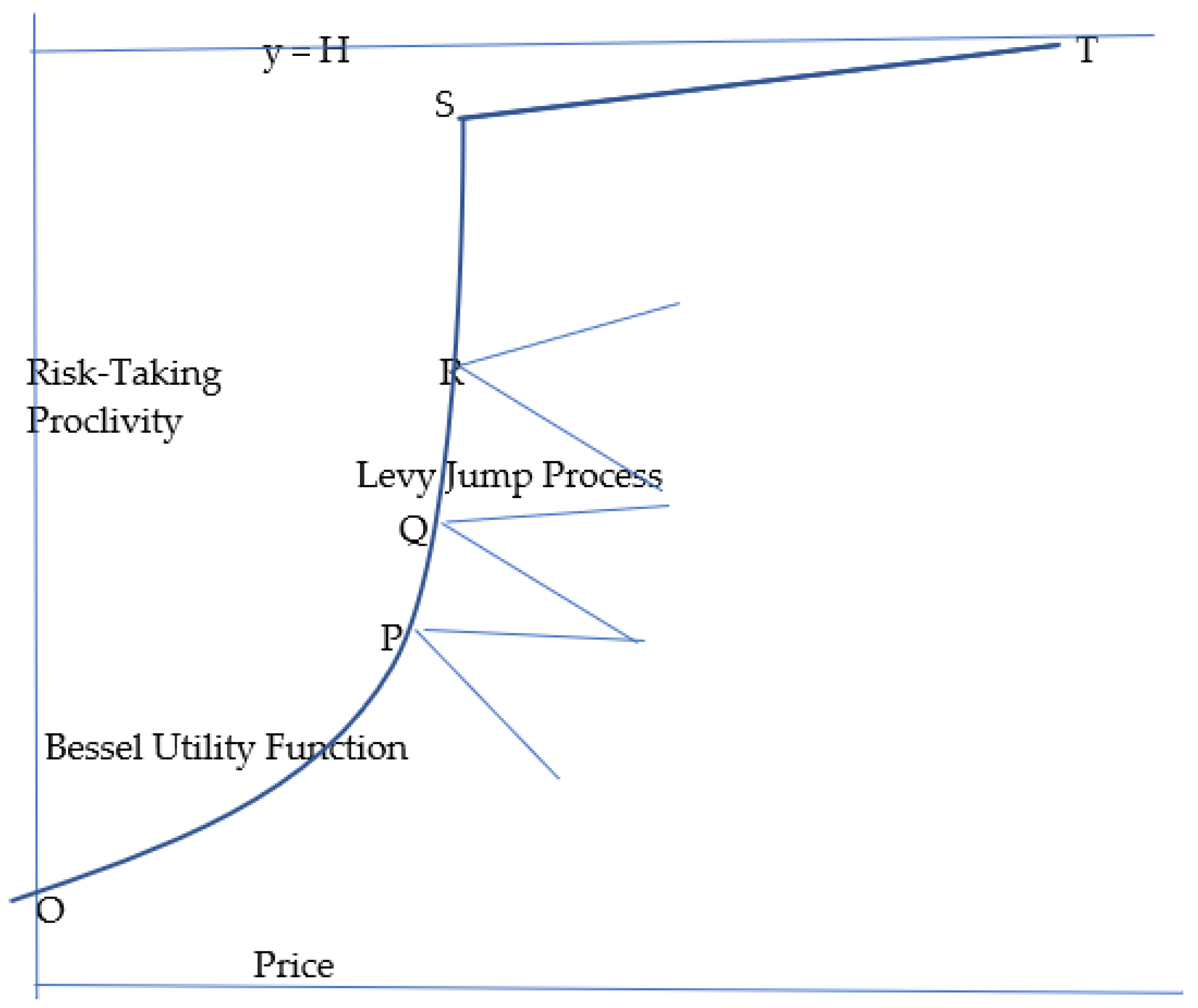
3.3. Valuation of Ether by the Risk-Taker

Subjects in experiments with gambling propensities were observed to take significantly higher investment risk in the purchase of stocks, bonds, certificates of deposit, or a house, or use of installment credit (Wong and Carducci 1991).
The risk-taker’s expectations can be modeled as a trader purchasing ether at higher and higher prices, with the expectation of increasing profits. After each purchase, news enters prices, which continue to rise. As prices of ether keep rising, the risk-taker reaches the maximum price, beyond which he or she cannot pay an additional amount.
In the formulation below, this desire for risk is approximated by a Bessel function (Equation (9)). The upper limit is achieved at Y = H, at which traders are not willing to pay any additional amount in pursuit of higher ether prices. Figure 3 is a graphical depiction of the risk-taker’s pricing of ether.

The Objective Function and Constraints

Objective Function. The three parts of the objective function consist of (1) the asymptotic expansion of the Bessel function of investor expectations, (2) a gamma distribution of the transformative attributes of cryptocurrencies, and (3) a Legendre integral describing the surpassing of bitcoin by ether. The objective function of the model to value ether by the risk-taking investor is as follows:
M a x   [ J 0 ( t ) + i Y 0 ( t ) ] d t ~ ( 2 / Π x ) e ^ t   ( x Π / 4 ) ] x [ ( ) k a 2 k + 1 x 2 k 1 + i ( ) k a 2 h x 2 k ]   f o r   t h e   a s y m p t o t i c   e x p a n s i o n   o f   t h e   i n t e g r a l   o f   a   B e s s e l   f u n c t i o n ,
where
  • t = time,
  • x = the price of ether,
  • z = x + iy, x, y, v real numbers;
    + ( k 1 ) ln x i x i θ N ln ( θ ) N ln ( Γ ( k ) )   f o r   t h e   g a m m a   d i s t r i b u t i o n ,
where
  • k = shape parameter,
  • θ = scale parameter;
    + ( 1 z 2 ) d 2 w / d z 2 2 z d w / d z + [ v ( v + 1 ) μ 2 / ( 1 e 2 ) ] w + x 2
where
  • v = degree of the Legendre integral, usually 1, or 2,
  • μ = order of the Legendre integral, usually 1,
  • z = a real number in the interval, −1 ≦ x ≦ 1,
  • x 2 = gradient vector, to reduce ether’s risk as late mover.
Constraints. Equation (10) is the average of the buying and selling prices of ether, say in the first round of trading. Then, news enters prices, and prices rise in the second round of trading. When the trader refuses to pay more for ether, ether has achieved its highest trade price. This is seen at H in Equation (11).
T t . > ( B 1 + A ) / 2
T t = ( B 1 + A ) / 2 = H ( u p p e r   b o u n d )
where
  • Tt = trade price,
  • B1 = buying price,
  • A = selling price,
  • H = highest purchase price,
The risk-taker’s expectations of ether prices are modeled by the Kullback–Liebler divergence. The price of ether is revised to a higher level, as news, n, enters prices. The Kullback–Liebler divergence is modeled on the left side of Equation (12). The risk-taker ceases purchasing ether when he or she feels that ether prices are at their maximum at H, shown on the right side of Equation (12):
[ e x / x + n [ 1 + n / ( x + n ) 2 + n ( n 2 x ) / ( x + n ) 4 + n ( 6 x 2 8 n x + n 2 ) / ( x + n ) 6 + 0.36 n 4 ] = H
where
  • x = price of ether,
  • n = news that enters prices,
  • H = highest purchase price.
Figure 3. Valuation of ether by the risk-taker.
Jrfm 15 00591 g003
OS is the utility function of the risk-taker. ST is the upper bound of the price distribution. Optimal prices at P, Q, and R for the risk-taker satisfy the Bessel utility function and the Levy Jump Process.
The derivation of optimal ether values for the risk-taker is contained in Appendix C.

4. The Valuation of Ether Derivatives
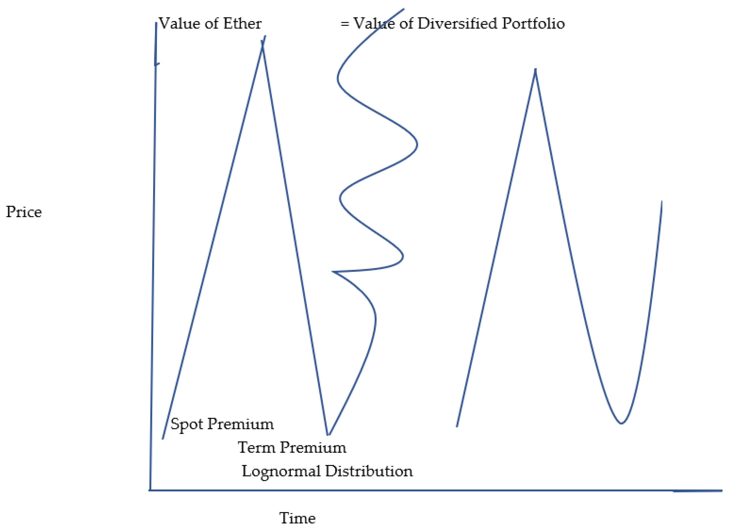
4.1. Futures

A futures contract on ether entitles the buyer to purchase ether at a fixed price, within a specified time-period. The current price is the spot price, whose fluctuation on the day of agreement is described by a lognormal distribution. Assume that actual purchase occurs in three months. The three-month interval between the initial contract date and final day of purchase is the delivery period. During the delivery period, prices of ether may change in jumps, or sharp, sudden increases. The price of ether futures is a combination of the spot price along with changes in the spot price, and the price during the delivery period along with changes in prices during the delivery period.

Objective Function and Constraints

Objective Function. There are four terms in the objective function. The investor maximizes gain by purchasing ether futures of high current and future value in Equation (13).
S p o t   P r e m i u m t 0   t o   t 1   [ e u + 0.5 σ 2 . φ [ ln ( k ) μ σ 2 σ ] [ 1 φ . [ ln ( k ) μ σ ] ] ] + T e r m   P r e m i u m t 1 t o [ γ t + B t + | x | s ( 0 , t ) x J x d s d x + | x | s { 0 , t } x J x d s d x + l i m ε | x | < 1 ,   | x | < 1 ,   ε [ 0 , t ] x J x ( d s d x v ( d x d s ) ] + s k 2 + k 2
The first term pertains to the current spot price, and the lognormal distribution of stock prices on the date of contract, as follows:
S p o t   P r e m i u m t 0   t o   t 1 [ e u + 0.5 σ 2 . φ [ ln ( k ) μ σ 2 / σ ] / [ 1 φ . [ ( ln ( k ) μ ) / σ ] ]
where
  • Spot Premium = price on the date of contract,
  • t1 = time-period 1, the day of entering into the contract,
  • μ = mean of the lognormal distribution,
  • σ = standard deviation of a lognormal distribution,
  • k = spot price of ether futures,
  • φ = constant.
The second term pertains to the term premium, the price paid for the fluctuation in ether futures prices during the three-month delivery period. To this amount, we add a Levy jump process, or a series of sharp increases in ether futures prices during the delivery period.
T e r m   P r e m i u m t 1 t o [ γ t + B t + | x | s ( 0 , t ) x J x d s d x
  • Term Premium = the price paid for the fluctuation in ether futures prices during the three-month delivery period,
  • t 1 t o   [ γ t + B t + | x | s ( 0 , t ) x J x d s d x = Levy jump process, or a series of sharp increases in ether futures prices during the delivery period,
  • x = price of ether futures,
  • s = change in ether futures price,
  • γ = size of jump,
  • B = constant,
The third term ibn the objective function is the degree of skewness of the distribution of ether futures prices, or the slope towards the far right or far left.
  • | x | s { 0 , t } x J x d s d x = skewness,
  • x = price of ether futures,
  • t = time, during the delivery period,
  • s = change in ether futures price,
The fourth term ibn the objective function is the degree of kurtosis, or flatness of the distribution of ether future prices.
  • x = price of ether futures,
  • t = time, during the delivery period,
  • s = change in ether futures price,
  • ε | x | < 1 ,   | x | < 1 ,   ε [ 0 , t ] x J x ( d s d x v ( d x d s ) ] = kurtosis of ether futures prices.
Constraints. The first constraint is that the term premium is higher than the spot premium (see Equation (14)).
S p o t   P r e m i u m t 0   t o   t 1 [ e u + 0.5 φ [ ln ( k ) μ σ 2 / σ ] / [ 1 φ [ ln ( k ) μ ) / σ ] ] < T e r m   P r e m i u m   t 1 t o [ γ t + B t + | x | 1 ,   s { 0 , t } x J x d s d x + l i m ε | x | < 1 ,   ε [ 0 , t ] x J x ( d s d x v ( d x d s ) ]
The second constraint is that the value of ether futures is more dependent on the term premium than the spot premium (see Equation (15)). The value of ether is the term premium − the spot premium, which is a positive amount,
V = V a l u e   o f   E t h e r = T e r m   P r e m i u m t 1 t o [ γ t + B t + | x | 1 ,   s { 0 , t } x J x d s d x + l i m ε | x | < 1 , ε [ 0 , t ] + x J x ( d s d x v ( d x d s ) ] S p o t   P r e m i u m t 0   t o   t 1 [ e u + 0.5 σ 2 φ [ ln ( k ) μ σ 2 / σ ] / [ 1 φ [ ln k μ ) / σ ] ] > 0
The third constraint states that the spot price x number of ether futures units, along with the term premium and ether futures units during the delivery period, is the value of ether.
S p o t   P r e m i u m V 1 + T e r m   P r e m i u m V 2 = V = V a l u e   o f   E t h e r
  • V1 = number of ether futures units at the spot price,
  • V2 = number of ether futures units at the delivery period price.
In Equation (16), the volatility of the term price on the left side is stipulated to be greater than the volatility of the spot price on the right side.
μVi = mean of the term price.
In Equation (17), the optimal volume of ether, which is the average of the spot volume and the term volume, (V1 + V2)/2 is equated to an alternative investment, which acts as the opportunity cost of foregoing ether futures (see Appendix D). The alternative investment is a diversified portfolio of with weights, w1, w2, …and returns r1, r2,…. This is an adaptation of the economic order quantity (EOQ) model for the determination of optimal order quantity for inventory, as ether future spot prices are valued as an inventory of cryptocurrencies.
t 1 [ ( V i μ V i j ) 2 ] / n 2 ( V 1 + V 2 ) / 2 = 2 V 1 / ( w 1 r 1 x 1 + w 2 r 2 x 2 )
Figure 4 shows the dynamics of ether futures price estimation presented in this model.

5. Findings and Analysis: The Valuation of Ether Options

Value of a Call Option on Ether

Assume that a recession is forecasted. Short-term interest rates exceed long-term rates. Investors will begin by purchasing ether call options, as they expect to gain from ether price increases. They also purchase put options, so that they will make gains if prices of ether decline. Then, they purchase short-maturity bonds that earn them high interest. When interest rates fall on the short-maturity bonds, investors sell them and purchase long-maturity bonds whose prices rise over time. Figure 5 shows the price movements and investor expectations of the objective function. Appendix E shows the mathematical achievement of optimal ether options values.
  • (Price of Ether Call×Fokker–Planck Equation of Upside Ether Call Trajectory) +
  • (Price of Ether Put×Fokker–Planck Equation of Downside Ether Put Trajectory) +
  • (Short Sale Price – Purchase Price on Bond 1) × Bond Price Path +
  • (Sales Price − Purchase Price on Bond 2) × Bond Price Path
Objective Function. The objective function is listed in Equation (18).
C [ t o d x i   t o   i   d x 1 / d Π 1 ( ε x 1 ( x 1 x 1 ) / ε   + x 1 D 1 ( x , t ) +   x 1 2 D 2 ( x , t ) ) p ( x , t ) + O ( ε 2 ) ] + P [ t o d x i   t o   i   d x 2 / d Π 2   ( ε x 2 ( x 2 x 2 ) / ε x 2 D 1 ( x , t ) x 2 2 D 2 ( x , t ) ) p ( x , t ) O ( ε 2 ) ] + ( S P B 1 P P B 1 ) * ( a 1 + b 1 x 1 ) + ( S S P P B 2 ) * ( a 2 + b 2 x 2 )
where
  • C [ t o d x i   t o   i   d x 1 / d Π 1 ( ε x 1 ( x 1 x 1 ) / ε + x 1 D 1 ( x , t ) = price trajectory of a call option,
  • C = price of a call option,
  • x1 = random variable of call prices,
  • x1′ − x1 = change in call values along the path,
  • D1(x,t) = diffusion coefficients of call values along the path in time periods, t1 and t2,
  • i   t o   i   d x 1 / d Π 1 ( ε x 1 ( x 1 x 1 ) / ε = a Fourier integral of incremental changes in call values,
  • P = price of a put option,
  • x2 = random variable of put prices,
  • x2′ − x2 = change in put values along the path,
  • D2(x,t) = diffusion coefficients of put values along the path in time periods, t1 and t2,
  • i   t o   i   d x 2 / d Π 2 ( ε x 2 ( x 2 x 2 ) / ε = a Fourier integral of incremental
  • changes in put values,
  • ( S P B 1 P P B 1 ) ( a 1 + b 1 x 1 ) = trajectory of bond prices for short-term bonds, (Short Sale Price − Purchase Price on Bond 1) on Bond 1,
  • ( S S B 2 P P B 2 ) ( a 2 + b 2 x 2 ) = Trajectory of bond prices for long term bonds, (Sales Price − Purchase Price on Bond 2) on Bond 2.
Constraints
( x 2 x 2 ) x 2 + ( x 3 x 3 ) x 3 + ( x 4 x 4 ) x 4 . > ( x 2 x 2 ) x 2 ( x 3 x 3 ) x 3 ( x 4 x 4 ) x 4
where
  • x values on the left of Equation (19) = ether prices, if ether prices increase,
  • x values on the right of Equation (19) = ether prices, if ether prices decrease.
where ether prices on the left side will rise by a larger amount than the ether price declines on the right side. Assuming that ether displaces bitcoin, with p > q, where p is the probability of ether displacing bitcoin, and q = 1 − p, the probability of bitcoin replacing ether, we apply de Moivre’s martingale, which increases p, the likelihood of ether displacing bitcoin. At the point of displacement, the second derivative of q/p reaches the limit, as shown in the Martingale Stopping Algorithm (Doob 1940) as shown in Equation (20).
E [ Y n + 1 | x n 1 X n + 1 ] = p ( q / p ) ( q / p ) ^ X n + q ( p / q ) ( q / p ) | X T ( φ ) | X 0 ( φ ) + k = 1   t o   X T ( φ ) | X k ( φ ) X k 1 ( φ ) X 0 ( φ ) + K T ( φ )
where
  • x = range of bitcoin prices,
  • p = probability of ether displacing bitcoin,
  • q = probability of bitcoin displacing ether,
  • Y = is the range of ether prices, given bitcoin prices, with the second derivative of the probability of ether displacing bitcoin, p at the maximum benefit of ether, so that the right side of Equation (20) = the incremental positive benefit from bitcoin’s continued use,
  • X k ( φ ) X k 1 ( φ ) is less than the benefit from using ether,
  • X k ( φ ) X k 1 ( φ )   φ = positive benefit from bitcoin’s continued use,
  • X 0 ( φ ) + K T ( φ ) = benefit from using ether,
  • ε = the incremental time interval over which the Fokker–Planck equation describing the path of call options holds.
Figure 5. Call option with a fixed-income arbitrage strategy.
Jrfm 15 00591 g005
An investor holds call options and put options long, while shorting certain bonds in favor of others with rising values. The price of the call option ascends along OP, while the price of the put option descends along QR. The bond has a relatively flat trajectory, AB.

6. Empirical Validation

Empirical validation of the five models in this paper is presented in this section. The first model, contained in Section 3.1, is the explanation of ether prices by the sentiments of risk-averse investors. We collected ether prices for 1 year, as the dependent variable. Investor sentiment was measured by the 3-period moving average of low prices, as risk-averse investors will be satisfied with low prices if they can avoid risk. Jumps are measured as the difference between closing prices. In Panel A of Table 1, the model for ether prices forecasted by the risk-averse investor is supported, with significant coefficients for investor sentiment, and jumps. The coefficient for risk-aversion is a highly significant value of 1.0 (t = 247, p < 0.001), while the coefficient for jumps is also highly significant at 0.56 (t = 27.1, p < 0.001). The second model, contained in Section 3.2, is the explanation of ether prices by the sentiments of moderately risk-taking investors. We collected ether prices for 1 year as the dependent variable. Investor sentiment was measured by the 3-period moving average of open prices, as moderately risk-taking investors will be satisfied with open prices if they can earn returns with a rational level of risk. Jumps are measured as the difference between closing prices. In Panel B of Table 1, the model for ether prices forecasted by the moderately risk-taking investor is supported, with significant coefficients for investor sentiment and jumps. The coefficient for moderate risk-taking is a highly significant value of 0.99 (t = 291, p < 0.001), while the coefficient for jumps is also highly significant at 0.66 (t = 37.8, p < 0.001). The third model, contained in Section 3.3, is the explanation of ether prices by the sentiments of risk-taking investors. We collected ether prices for 1 year, as the dependent variable.
Investor sentiment was measured by the 3-period moving average of high prices, as risk-taking investors will only be satisfied with high prices. Jumps are measured as the difference between closing prices. In Panel C of Table 1, the model for ether prices forecasted by the risk-taking investor is supported, with significant coefficients for investor sentiment, and jumps. The coefficient for risk-taking is a highly significant value of 0.98 (t = 271, p < 0.001), while the coefficient for jumps is also highly significant at 0.58 (t = 30.9, p < 0.001).
The fourth model, shown in Section 4, forecasts ether futures prices using investor sentiment and jumps. Ether futures prices were collected on an intraday basis during January–May 2022. Trading volume of the volume of ether futures bought or sold measured investor sentiment as optimism for buys and pessimism for sells. Jumps were measured as the difference between ether futures closing prices. Corrections for heteroscedastic residuals were applied. Panel D of Table 1 shows that this model was supported, with significant coefficients for investor sentiment and jumps. The coefficient of investor sentiment is a highly significant value of −0.02 (t = −2.87, p < 0.01), while the coefficient for jumps is marginally significant at 0.0008 (t = 0.18, p < 0.1).
The fifth model, shown in Section 5, forecasts ether call options prices using investor sentiment and jumps. Ether call option prices were collected on an intraday basis during January–May 2022. Trading volume of the volume of ether calls bought or sold measured investor sentiment as optimism for buys, and pessimism for sells. Jumps were measured as the difference between call closing prices. Corrections for heteroscedastic residuals were applied. Panel E of Table 1 shows that this model was supported, with significant coefficients for investor sentiment and jumps. The coefficient of investor sentiment is a highly significant value of −5.28 (t = −2.70, p < 0.01), while the coefficient for jumps is significant at 2.05 (t = 2.15, p < 0.05).

7. Conclusions

This paper fulfilled its objective of providing a theoretical valuation of ether and ether derivatives. We believe that ether prices are driven by investor sentiment and price jumps. Investor sentiment differs for risk-averse investors, moderate risk-takers, and risk-takers. Price jumps are price breaks during which ether prices suddenly rise. We have mathematically formulated ether valuations for the three types of investors. We specify utility function formulations drawn from advanced exponential functions, as we believe that utility theory must be represented in its complexity. Attitudes to risk are rarely simple, being at the confluence of multiple forces. The literature on cryptocurrency is dominated by articles on bitcoin, as the market leader. This study is an early theoretical formulation of the valuation of the late mover, ether. The basic economic theory of determinants of demand for ether is supplemented by the strategic management theory of first movers and late movers. We draw on Yip’s (1982) observation that a late mover, like ether, can exploit technological discontinuities overlooked by the first mover. However, we render our models to be realistic by accounting for the fact that, in some cases, a first-mover such as bitcoin could make a resurgence.
We offer additional formulations to price ether derivatives, including ether futures and ether options. The future formulation’s pegging of ether futures to the Australian dollar eliminates much of the ether-to-US dollar conversion risk, in that the Australian dollar maintains strength and stability. For ether options, we offer a combined put-call strategy to maximize gains, while limiting risk.
Future research must create theoretical formulations for litecoin and peercoin, which are lesser-known cryptocurrencies. Abraham (2019) suggested the creation of a new measure of risk-aversion to replace the Arrow–Pratt measure, which is over fifty years old. This may result in a 5-scale classification of risk-aversion, risk avoider, risk-averse, moderate risk-taker, somewhat moderate risk-taker, and risk-taker. For the risk-taker, a measure that includes gambling is suggested, as initial success from risky investment stimulates the desire for further risk-taking.

Author Contributions

Conceptualization: R.A. and H.E.-C.; Mathematical Formulation: R.A.; Validation: H.E.-C. Writing—Review or Editing: R.A.; Visualization: R.A.; Supervision: H.E.-C.; Project Administration: H.E.-C. We confirm that neither the manuscript, nor any parts of its content are currently under consideration or published in another journal. All authors have read and agreed to the published version of the manuscript.

Funding

This research received no external funding.

Data Availability Statement

Data are available upon request.

Conflicts of Interest

The authors declare no conflict of interest.

Appendix A

The optimal price for the risk-averse investor is as follows:
Z Taking Lagrangians of Equations (A1)–(A4),
M a x   ( 1 + λ ) [ 1 exp ( α   γ   x ) ] λ [ 1 exp ( α   γ   x ) 2 ] x 1 / θ N k ln θ ( Γ k ) + . ( 1 z 2 ) d 2 w / d z 2 3 z d w / d z + [ v ( v + 1 ) μ 2 / ( 1 e 2 ) ] w + x 2 L 1 [ x 1 + x 2 + x 3       . x 4 y 1 y 2 y 3 y 4 ] L 2 [ γ t + B t + | x | 1 ,   s { 0 , t } x J x ( d s d x ) + | x | 1 ,   s { 0 , t } x J x ( d s d x ) + l i m ε | x | < 1   ε [ 0 , t ] x J x ( d s d x ) v ( d x d s ) H ] L 3 [ 0.5 ρ 2 s 2 ( 1 / 6 ) ρ ρ   . s 3 [ ρ 2 3 ρ ( m e a n ) 2 + ρ ( m e a n ) ] s s s s / 24 ρ ρ ρ ρ ρ [ α [ s s 3 / 6 ρ 2 . s 3 . + { ρ ( m e a n ) / 8 ρ 4 s 4 } { ρ ( m e a n ) / 8 ρ 4 s 4 } b [ s s s s ρ 2 + ρ ( m e a n ) / 8 ρ 4 s 4 H   .
The necessary condition for optimization of the value of ether is the first derivative of the maximization function, as shown in Equation (A2).
( 1 + λ ) [ 1 + exp ( α   γ   x ) x i / θ Nk / θ N / Γ ( k ) 2 zd 3 / dz 3 2 d 2 w / d z 2 + . [ v ( v + 1 ) μ 2 / ( 1 e 2 ) L 1 [ 3 y 1 y 2 y 3 y 4 ] L 2 [ d γ t / d x + d B t / d x + x J x   . + x J x + x d x v H ] L 3 [ s / ρ ] [ ( ρ 2 s 2 / 18 ] [ 3 ρ ( m e a n ) 2 + ρ ( m e a n ) ] 4 s 3 / 6 ρ 5 ] . 2 a [ s s 3 / 6 ρ 2 + { ρ ( m e a n ) s 4 / 8 ρ 4 } b [ 1 3 s 2 / ρ 2 + { ρ ( m e a n ) / 8 ρ 4 } 4 / 3 s 3 ] = 0   .
The sufficient condition for optimization of the value of ether is the second derivative of the maximization function equated to 0, as shown in Equation (A3).
( 1 + λ ) [ 1 2 exp ( α   γ   x ) 3 + 2 [ exp ( α   γ   x ) ] 1 / θ Nk / θ N / Γ ( k ) 2 zd 4 / dz 4 2 d 3 w / d z 3 + . [ v ( v + 1 ) μ 2 / ( 1 e 2 ) ] + x 2 L 1 [ y 1 y 2 y 3 y 4 ] L 2 [ d 2 γ t / d x 2 + d 2 B t / d x 2 + 2 J x + 1   . v H ] L 3 [ 1 / ρ ] [ ( ρ 2 s 3 / 9 ] [ 3 ρ ( m e a n ) 2 + 12 ρ ( m e a n ) ] s 2 / 6 ρ 5 ] . 2 a [ 1 3 s 2 / 6 ρ 2 + { 4 ρ ( m e a n ) s 3 / 8 ρ 4 } b [ 1 6 s / ρ 2 + { ρ ( m e a n ) / 8 ρ 4 } 4 s 2 ] = 0 .
Figure 1 shows optimal prices as P, Q, and R obtained by iteratively solving Equation (A4) for x;
2 exp ( α   γ   x ) = [ 1 1 / θ N k / θ N / Γ ( k ) 2 d 4 w / d z 4 2 d 3 w / d z 3 + [ v ( v + 1 ) . μ 2 / ( 1 e 2 ) ] ( 1 / ( 1 + λ ) . L 1 [ y 1 y 2 y 3 y 4 ] 1 / ( 1 + λ ) . L 2 [ d 2 γ t / d x 2   . + d 2 B t / d x 2 + 2 J x v H ] ( 1 / ( 1 + λ ) L 3 [ 1 / ρ + ρ 2 s 3 / 9 ( 3 ρ mean ) 2   . + ρ ( m e a n ) / ρ s ] 2 s s 2 a [ 1 3 s 2 / 6 ρ 2 + { ρ ( m e a n ) s 3 / 2 ρ 4 } b [ 6 s 2 / ρ 2   . + { ρ ( m e a n ) / 8 ρ 4 } 4 s s ] .

Appendix B

The derivation of the optimal value of ether for the moderate risk-taker is as follows.
Taking Lagrangians,
( 1 + λ ) [ 1 exp ( α   γ   x ) ] α λ [ 1 exp ( α   b   x ) a ] α > 0   | λ 1 | + ( k 1 ) ln x i . x i N k ln θ N ln ( Γ ( k ) ) + ( 1 z 2 ) d 2 / d z 2 2 z d w / d z + [ v ( v + 1 ) . μ 2 / ( 1 e 2 ) ] w + x 2 L 1 [ x 1 + x 2 + x 3 + x 4 y 1 y 2 y 3 y 4 ] L 2 [ γ t + B t + x J x d s d x + x J x d s d x + l i m x { J x ( d s d x ) v ( d x d s ) } = ( 0.2 r 1 + 0.08 r 2 + 0.12 r 3 + 0.2 r 4 + 0.4 r 5 ) ] . L 3 [ [ ( 0.5 s 2 / ρ ( ρ / 6 ρ 3 s 3 ] [ ρ 2 3 ρ ( m e a n ) 2 + ρ ( m e a n ) ] s 4 / 24 ρ 5 . [ a [ s s 3 / 6 ρ 2 + { ρ ( m e a n ) / 8 ρ 4 s 4 / 24 ρ 5 [ a [ s 1 / 6 ρ 2 s 3 + . ρ ( m e a n ) ] s s s s / 24 . ρ ρ ρ ρ ρ ] ^ 2 b [ s s 3 / ρ 2 + { ρ ( m e a n ) / 8 ρ 4 ] s ^ 4   ] . L 4 [ e x / n + n { 1 + n / ( x + n ) 2 + n ( n 2 x ) / ( x + n ) 4 + n ( 6 x 2 8 n x + n 2 ) / . ( x + n ) 6 + 0.36 n 4 ] L 5 [ [ m 2 / 3 m 1 1 ] / [ θ 2 2 θ + ( θ 3 3 θ 2 + 3 θ ) m 2 / 3 m 1 ] ] .
The necessary condition for optimization of the objective function is the first derivative,
( 1 + λ ) [ 1 + exp ( α   γ   x ) ] 2 α λ [ 1 + exp ( α   b   x ) a 1 ] + ( k 1 ) ln x x i / θ N k / θ   . N / Γ ( k ) + ( 1 z 2 ) d 3 w / d w 3 2 z d 2 w / d z 2 + [ v ( v + 1 ) μ 2 / ( 1 e 2 ] + 2 x ]   . L 1 [ 4 y 1 y 2 y 3 y 4 ] L 2 [ γ + B + J x + J x } L 3 [ ( s / ρ ) [ 1 / 18 ρ 2 ] . [ ρ 2 3 ρ ( m e a n ) 3 + ρ ( m e a n ) / 24 ρ 5 ] 4 s s s + L 4 ( e x + n ( 12 x 8 n + n 2 ) / 6 ( x + n ) 5 . + 0.36 n 4 ] m 2 / 3 m 1 / [ θ 2 3 θ 2 + 3 θ ] m 2 / 3 m 1 = 0 .
The sufficient condition for the optimization of the objective function is the second derivative,
( 1 + λ ) [ 2   exp ( α   γ   x ) ] 3 α λ [ ( a 1 ) 1 exp ( α   b   x ) a 2 ] + ( k 1 ) / x 1 / θ N k / θ   . N / Γ ( k ) + ( 2 z d 4 w / d w 4 2 z d 3 w / d z 3 + 2 x ]   . L 1 [ y 1 y 2 y 3 y 4 ] L 2 [ γ t + B t + J x + J x } L 3 [ ( 1 / ρ ) [ 9 ρ ( m e a n ) ] 12 s 2 . 2 a [ s / ρ 2 + 3 ρ ( m e a n ) s 2 / 2 ρ 4 ] b [ ( 6 s / ρ 2 + m e a n / 8 ρ 3 ) ] ^ 0.5 + L 4 . ( e x + n ( 12 8 n + n 2 ) / 30 ( x + n ) 4 1.44 n 5   . m 2 / 3 m 1 / ( θ 2 3 θ 2 + 3 θ ) m 2 / m 1 = 0 .

Appendix C

The derivation of the optimal value of ether for the risk-taker is as follows.
Taking Lagrangians,
[ J 0 ( t ) + i Y 0 ( t ) ] d t ~ ( 2 Π x ) 0.5 e t x Π 4 x [ ( ) k a 2 k + 1 x 2 k 1 + i ( ) k a 2 h x 2 k ] + [ x i θ N k ln ( θ ) N ln ( Γ ( k ) ] + [ ( 1 z 2 ) d 2 w d z 2 2 z d w d z + v ( v + 1 ) μ 2 ( 1 e 2 ) w ] + 𝛻 x 2 L 1 ( x 1 + x 2 + x 3 + x 4 y 1 y 2 y 3 y 4 ) L 2 [ γ t + B t + | x | 1 ,   s { 0 , t } x J x ( d s d x ) + | x | < 1 ,   s { 0 , t } x J x ( d s d x ) + l i m ε | x | < 1 ,   ε [ 0 , t ] x J x ( d s d x v d x d s ) ] L 3 [ T t B 1 + A 2 ] L 4 [ T t B 1 + A 2 ] H ) L 5 [ e x / x + n { 1 + n / ( x + n 2 + n ( n 2 x ) ( x + n ) 4 + n ( 6 x 2 8 n x + n 2 ) ( x + n ) 6 + 0.36 n 4 ] 0.5 H L 6 [ ( log x 1 ( d P 1 d Q 1 ) d P 1 d Q 1 d Q 1 + log x 2 ( d P 2 d Q 2 ) d P 2 d Q 2 d Q 2 + log x 3 ( d P 3 d Q 3 ) d P 3 d 3 d Q 3 )   γ t B t | x |     1 ,   s { 0 , t } x J x ( d s d x ) | x | < 1 ,   s { 0 , t } x J x ( d s d x ) + l i m [ ε | x | < 1 , ε [ 0 , t ] x { J x ( d s d x ) v ( d x d s ) }
The necessary condition for the optimization of ether prices is the first derivative of the Lagrangian in Equation (A6);
[ J 0 ( t ) + i Y 0 ( t ) ] d t ~ ( 2 Π x ) 0 . 5 e t x Π 4 x [ ( ) k a 2 k + 1 x 2 k 1 + i ( ) k a 2 h x 2 k ] + [ x i θ N k / ( θ ) N ( Γ ( k ) ] + [ ( 1 z 2 ) d 3 w d z 3 2 z d 2 w d z 2 + v ( v + 1 ) μ 2 ( 1 e 2 ) w ] + 2 𝛻 x L 1 ( 4 y 1 y 2 y 3 y 4 ) L 2 [ γ t + B t + 2 J x + x J x ( d s d x ) v d x d s ] L 3 [ 1 B 1 + A 2 ] L 4 [ B 1 + A 2 ] ) + L 5 [ e x + n { n / 2 ( ( x + n ) + n ( n 2 ) 4 ( x + n ) 3 + n ( 12 x 8 n x + n 2 ) 6 ( x + n ) 5 ] 0.5 L 6 [ ( log ( d P 1 d Q 1 ) d P 1 d Q 1 + log ( d P 2 d Q 2 ) d P 2 d Q 2 + log ( d P 3 d Q 3 ) d P 3 d Q 3 ) γ t B t 2 J x + x J x { ( d s d x ) v ( d x d s ) } ]
The sufficient condition for the optimization of ether is the second derivative of the Lagrangian function in Equation (A7);
[ J 0 ( t ) + i Y 0 ( t ) ] d t ~ ( 2 Π x ) 0 . 5 e t x Π 4 [ ( ) k a 2 k + 1 ( 2 k 1 ) x 2 k 2 + i ( ) k a 2 h ( 2 k ) x 2 k 1 ] + [ 1 / θ N k / ( θ ) N ( Γ ( k ) ] + [ ( 1 z 2 ) d 4 w d z 4 2 z d 3 w d z 3 + v ( v + 1 ) μ 2 ( 1 e 2 ) w ] + 2 L 1 ( y 1 y 2 y 3 y 4 ) L 2 [ γ t + B t + 2 J x + x J x ( d s d x ) v d x d s ] L 3 [ B 1 + A 2 ] L _ 4   [ B 1 + A 2 ] ) + L 5 [ e x + n { n / 2 ( ( 1 + n ) + n ( n 2 ) 8 ( x + n ) + n ( 12 8 n + n 2 ) 30 ( x + n ) 4 ] 0.5 L 6 [ ( log ( d Q 1 d P 1 ) d 2 P 1 d 2 Q 1 + log ( d Q 2 d P 2 ) d 2 P 2 d 2 Q 2 + log ( d Q d P 3 ) d 2 P 3 d Q 3 2 ) ] γ t B t 2 J x + ( { J x ( d s d x ) v ( d x d s ) } ]

Appendix D

The optimal ether futured price is as follows.
Taking Lagrangians,
S p o t   P r e m i u m t 0 t o   t 1 [ e u + 0.5 σ 2 . φ [ ln ( k ) μ σ 2 / σ ] / [ 1 φ . [ ( ln ( k ) μ ) / σ ] ] + T e r m   P r e m i u m t 1 t o [ γ t + B t + | x | s ( 0 , t ) x J x d s d x + | x | s { 0 , t } x J x d s d x + l i m ε | x | < 1 ,   | x | < 1 , ε [ 0 , t ] x J x ( d s d x v ( d x d s ) ] + s k 2 + k 2 L 1 [ S p o t   P r e m i u m t 0 t o   t 1 [ e u + 0.5 φ [ ln ( k ) μ σ 2 / σ ] / [ 1 φ [ ln ( k ) μ ) / σ ] ]   T e r m     P r e m i u m t 1 t o [ γ t + B t + | x | 1 ,   s { 0 , t } x J x d s d x + l i m ε | x | < 1 ,   ε [ 0 , t ] x J x ( d s d x v d x d s ] L 2 [ T e r m   P r e m i u m t 1 t o [ γ t + B t + | x | 1 ,   s { 0 , t } x J x d s d x + l i m ε | x | < 1 ,   ε [ 0 , t ] + x J x ( d s d x v ( d x d s ) ] S p o t   P r e m i u m t 0 t o   t 1 [ e μ + 0.5 σ 2 φ [ ln ( k ) μ σ 2 / σ ] / [ 1 φ [ ln k μ ) / σ ] ]   L 3 [ S p o t   P r e m i u m V 1 + T e r m   P r e m i u m V 2 ] L 4 [ t 1 [ ( V i μ V i j ) 2 ] / n 2 [ ( V 1 + V 2 ) / 2 2 V 1 / ( w 1 r 1 x 1 + w 2 r 2 x 2 . ) ]
The necessary condition for optimization is
M a x   S p o t   P r e m i u m [ e ^ μ + 0.5 σ 2 φ [ ln ( k ) μ σ 2 / σ ] / [ 1 φ [ ln k μ / σ ] ] + T e r m   P r e m i u m [ γ t + B t + 2 x J x + x J x ( d s d x v d x d s ) ] + 3 ( x μ ) 2 / σ + 4 ( x μ ) 3 / σ L 1 [ S p o t   P r e m i u m e μ 0.5 σ 2 φ [ ln ( k ) μ σ 2 / σ ] / [ 1 φ ( ln k μ / σ ) ] T e r m   P r e m i u m [ ( γ t + B t + 2 x J x ) ] + x J x [ ( 1 v ) + 6 ( x μ ) / σ + 12 ( x μ ) / σ ] L 2 [ T e r m   P r e m i u m [ γ t + B t + 2 x J x + x J x ( 1 v ) S p o t   P r e m i u m [ e ^ μ + 0.5 σ 2 φ ( ln ( k ) ( μ σ 2 / σ ) / [ 1 φ [ ( 1 / k μ ) / σ ) ] L 3 [ S p o t   P r e m i u m   d V 1 / d x + T e r m   P r e m i u m   d V 2 / d x ] L 4 [ ( V t μ V i ) 2 ] / n 2 [ ( V 1 + V 2 ) / 2 2 V 1 / ( w 1 r 1 x 1 + w 2 r 2 x 2 . ) ]
The sufficient condition for optimization is
M a x   S p o t   P r e m i u m [ e ^ μ + 0.5 σ 2 φ [ 1 / k 2 ( μ σ ) / σ ] / [ 1 φ [ 1 / k 2 ( μ σ ) / σ ] ] + T e r m   P r e m i u m [ γ t + B t + 2 J x + J x ( d s d x v d x d s ) + 6 ( x μ ) / σ + 12 ( x μ ) 2 / σ L 1 [ S p o t   P r e m i u m e μ 0.5 σ 2 φ [ 1 / k 2 ( μ σ ) / σ ] / [ 1 φ ( 1 / k 1 / σ ) ] T e r m   P r e m i u m [ ( γ t + B t + 2 J x ) ] + J x [ ( 1 v ) + 6 ( 1 μ ) / σ + 12 ( 1 μ ) / σ ] L 2 [ T e r m   P r e m i u m [ γ t + B t + 2 J x + J x ( 1 v ) S p o t   P r e m i u m [ e ^ μ + 0.5 σ 2 φ [ 1 / k 2 ( μ σ / σ ) / [ φ [ ( 1 / k 1 ) / σ ) ] L 3 [ S p o t   P r e m i u m   d 2 V 1 / d x 2 + T e r m   P r e m i u m   d 2 V 2 / d x 2 ] L 4 [ ( V t μ V i ) 2 ] / n 2 [ ( d V 1 / d x + d V 2 / d x ) / 2 1 / 2 V 1 ( w 1 r 1 + w 2 r 2 . ) ]

Appendix E

The optimal ether options price is as follows.
Taking Lagrangians,
C [ t o d x i   t o   i   d x 1 / d Π 1 ( ε x 1 ( x 1 x 1 ) / ε + x 1 D 1 ( x , t ) + x 1 2 D 2 ( x , t ) ) p ( x , t ) + O ( ε 2 ) ] + P [ t o d x i   t o   i   d x 2 / d Π 2 ( ε x 2 ( x 2 x 2 ) / ε x 2 D 1 ( x , t ) x 2 2 D 2 ( x , t ) ) p ( x , t ) O ( ε 2 ) ] + ( S P B 1 P P B 1 ) ( a 1 + b 1 x 1 ) + ( S S P P B 2 ) ( a 2 + b 2 x 2 ) L 1 [ ( x 2 x 2 ) x 2 + ( x 3 x 3   ) x 3 + ( x 4 x 4 ) x 4 . > ( x 2 x 2 ) x 2 ( x 3 x 3   ) x 3 ( x 4 x 4 ) x 4 ] L 2 [ t o d x i   t o   i   d x 1 / d Π 1 ( ε x 1 ( x 1 x 1 ) / ε + x 1 D 1 ( x , t ) + x 1 2 D 2 ( x , t ) ) p ( x , t ) + O ( ε 2 ) ] L 3 [ μ ( x , t ) a + σ 2 ( x t , t ) 2 b ( x 1 μ 1 σ 1 ) 3 ( x 1 μ 1 σ 1 ) 4 ( x 2 x 1 x 1 ) t 1 ( x 3 x 2 x 2 ) t 2 ( x n x n 1 n ) t n ]
The necessary condition for optimization is the first derivative of Equation (A10);
C [ d x 1 / d Π 1 ( ε x 1 ( x 1 x 1 ) / ε + x 1 D 1 ( x , t ) + x 1 2 D 2 ( x , t ) ) p ( x , t ) + O ( ε 2 ) ] + P [ d x 2 / d Π 2 ( ε x 2 ( x 2 x 2 ) / ε x 2 D 1 ( x , t ) x 2 2 D 2 ( x , t ) ) p ( x , t ) O ( ε 2 ) ] + ( S P B 1 P P B 1 ) ( a 1 + b 1 ) + ( S S P P B 2 ) ( a 2 + b 2 ) L 1 d / d x [ ( x 2 x 2 ) x 2 + ( x 3 x 3   ) x 3 + ( x 4 x 4 ) x 4 . > ( x 2 x 2 ) x 2 ( x 3 x 3   ) x 3 ( x 4 x 4 ) x 4 ] L 2 [ d x 1 / d Π 1 ( ε x 1 ( x 1 x 1 ) / ε + x 1 D 1 ( x , t ) + x 1 2 D 2 ( x , t ) ) p ( x , t ) + O ( ε 2 ) ] L 3 d / d x [ μ ( x , t ) a + σ 2 ( x t , t ) 2 b ( x 1 μ 1 σ 1 ) 3 ( x 1 μ 1 σ 1 ) 4 ( x 2 x 1 x 1 ) t 1 ( x 3 x 2 x 2 ) t 2 ( x n x n 1 n ) t n ]
The sufficient condition for optimization is the second derivative of Equation (A11);
C [ d 2 x 1 / d Π 1 2 ( ε 1 ( x 1 1 ) / ε + D 1 ( x , t ) + 2 x 1 D 2 ( x , t ) ) p ( x , t ) + O ( ε 2 ) ] + P [ d ^ 2   x 2 / d Π 2 ^ 2   ( ε 1 ( x 2 1 ) / ε D 1 ( x , t ) 2 x 2 D 2 ( x , t ) ) p ( x , t ) O ( ε 2 ) ] + ( S P B 1 P P B 1 ) + ( S S P P B 2 ) L 1 d 2 / d x 2 [ ( x 2 x 2 ) x 2 + ( x 3 x 3   ) x 3 + ( x 4 x 4 ) x 4 . > ( x 2 x 2 ) x 2 ( x 3 x 3   ) x 3 ( x 4 x 4 ) x 4 ] L 2 [ d x 2 1 / d Π 1 2 ( ε ( x 1 1 ) / ε + D 1 ( x , t ) + 2 x 1 D 2 ( x , t ) ) p ( x , t ) + O ( ε 2 ) ] L 3 d 2 / d x 2 [ μ ( x , t ) a + σ 2 ( x t , t ) 2 b ( x 1 μ 1 σ 1 ) 3 ( x 1 μ 1 σ 1 ) 4 ( x 2 x 1 x 1 ) t 1 ( x 3 x 2 x 2 ) t 2   ( x n x n 1 n ) t n ]

References

  1. Abraham, Rebecca. 2018. Pricing currency call options. Theoretical Economics Letters 8: 2569–93. [Google Scholar] [CrossRef] [Green Version]
  2. Abraham, Rebecca. 2019. Hedge fund investing or mutual fund investing: An application of multi-attribute utility theory. Theoretical Economics Letters 9: 605–32. [Google Scholar] [CrossRef] [Green Version]
  3. Bain, Benjamin. 2018. Ether Futures Likely Stalled as CFTC Launches Review of Token. Available online: https://www.bloomberg.com/news/articles/2018-12-11/ether-futures-likely-stalled-as-cftc-launches-review-of-token (accessed on 1 June 2020).
  4. Brunnermeir, Markus K., and Stefan Nagel. 2004. Hedge funds and the technology bubble. Journal of Finance 59: 2013–40. [Google Scholar] [CrossRef] [Green Version]
  5. Burgrraf, Tobias, Toan Luu Duc Huynh, Markus Rudolf, and Mei Wang. 2020. Do FEARS drive bitcoin? Review of Behavioral Finance 13: 239–58. [Google Scholar] [CrossRef]
  6. Burnside, Craig, Isaac Kleshchelski, and Sergio Robelo. 2006. The Returns to Currency Speculation. Working Paper, No. 12489. Cambridge: National Bureau of Economic Research. [Google Scholar]
  7. Cespa, Giovanni, and Xavier Vives. 2012. Dynamic trading and asset prices. The Review of Economic Studies 79: 539–80. [Google Scholar] [CrossRef] [Green Version]
  8. Chen, Joseph, Harrison Hong, and Jeremy C. Stein. 2002. Breadth of ownership and stock returns. Journal of Financial Economics 66: 171–205. [Google Scholar] [CrossRef] [Green Version]
  9. Cox, John C., Jonathan E. Ingersoll, and Stephen A. Ross. 1981. A reexamination about traditional hypotheses about the term structure of interest rates. Journal of Finance 36: 769–99. [Google Scholar] [CrossRef]
  10. Doob, Joseph L. 1940. Regularity properties of certain families of chance variables. Transactions of the American Mathematical Society 47: 455–86. [Google Scholar] [CrossRef]
  11. Easley, David O., Maureen O’Hara, and Pulle Subrahmanya Srinivas. 1998. Option volume and stock prices: Evidence on where informed traders trade. Journal of Finance 53: 431–65. [Google Scholar] [CrossRef]
  12. Eom, Cheolijun, Taisei Kaizoji, Sang Hoon Kang, and Lukas Pichl. 2019. Bitcoin and investor sentiment: Statistical characteristics and predictability. Physica A: Statistical Mechanics and Its Applications 514: 511–21. [Google Scholar] [CrossRef]
  13. Fama, Eugene F. 1984. Forward and spot exchange rates. Journal of Monetary Economics 4: 319–38. [Google Scholar] [CrossRef]
  14. Garcia, David, and Frank Schweitzer. 2015. Social signals and algorithmic trading of bitcoin. Royal Society Open Science 2: 1–13. [Google Scholar] [CrossRef] [PubMed] [Green Version]
  15. Garcia, David, Claudio J. Tessone, Pavlin Mevrodiev, and Nicholas Perony. 2014. The digital traces of bubbles: Feedback cycles between socio-economic signals in the Bitcoin economy. Journal of Royal Society Interface 11: 20140623. [Google Scholar] [CrossRef] [PubMed]
  16. Gorton, Gary B., Fumio Hayashi, and K. Geert Rouwenhorst. 2012. The Fundamentals of Commodity Futures Returns. Working Paper. New Haven: Yale University. [Google Scholar]
  17. Harrison, John Michael, and David C. Kreps. 1978. Speculative investor behavior in a stock market with heterogeneous expectations. Journal of Economics 92: 323–36. [Google Scholar] [CrossRef] [Green Version]
  18. Hayes, Adam S. 2017. Cryptocurrency value formation: An empirical study leading to a cost of production model for valuing bitcoin. Telematics and Informatics 34: 1308–21. [Google Scholar] [CrossRef]
  19. Ishanti, Marco, and Karim R. Lakhani. 2017. The truth about blockchain. Harvard Business Review 95: 118–27. [Google Scholar]
  20. Kent, Damiel, and David Hirshleifer. 2015. Overconfident investors, predictable returns, and excessive trading. The Journal of Economic Perspectives 29: 61–87. [Google Scholar]
  21. Keynes, John Maynard. 1936. The General Theory of Employment, Interest, and Money. London: Palgrave MacMillan. [Google Scholar]
  22. Kristoufek, Ladislav. 2013. Bitcoin meets Google Trends and Wikipedia: Quantifying the relationship between phenomena of the Internet era. Scientific Reports 3: 3415–20. [Google Scholar] [CrossRef] [Green Version]
  23. Lam, Eric, and David Wee. 2017. Bitcoin prices bubble-like after rally: Blackrock. Bloomberg Wire Services, December 1–2, 1–3. [Google Scholar]
  24. Leiberman, Marvin B., and David B. Montgomery. 1988. First-mover advantages. Strategic Management Journal 9: 44–58. [Google Scholar] [CrossRef]
  25. Levy, Ari, and Mackenzie Sigalos. 2022. Crypto Peaked a Year Ago-Investors Have Lost More Than $2 Trillion Since. Available online: cnbc.com/2022/11/11/crypto-peaked-in-nov-2021-investors-lost-more-than-2trillion-since.html (accessed on 12 December 2021).
  26. Malwa, Sri. 2018. Ethereum: Cashing out Fears Drive Falling Ether Prices, Protocol Co-Founder Refutes Worries. Available online: https://crytoslate.com/ethereum-cashing-out-fears-drive-falling-ether-prices-protocol-co-founder-refutes-worries (accessed on 12 December 2021).
  27. Merovci, Faton, Morad Alizadeh, and Gholamhossein Hamedani. 2016. Another generalized transmuted family of distributions: Properties and applications. Austrian Journal of Statistics 45: 71–93. [Google Scholar] [CrossRef] [Green Version]
  28. Mian, Mujtaba G., and Srinivasan Sankaraguruswamy. 2012. Investor sentiment and stock market response to earnings news. The Accounting Review 87: 1357–84. [Google Scholar] [CrossRef]
  29. Miller, Edwin. 1977. Risk, uncertainty, and divergence of opinion. Journal of Finance 32: 1151–68. [Google Scholar] [CrossRef]
  30. Nasir, Mohammad A., Toan Luu Duc Huynh, Sang Phu Nguyen, and Day Duong. 2019. Forecasting cryptocurrency returns and volume using search engines. Financial Innovation 5: 25. [Google Scholar] [CrossRef]
  31. Oxford Analytics Daily Brief Services. 2018. China: Firms Expect Bright Future for Blockchain. Available online: https://search-proquest.com/ezproxylocallibrary.nova.edu (accessed on 12 December 2021).
  32. Park, Andreas, and Hamid Sabourian. 2011. Herding and contrarian behavior in financial markets. Econometrica 79: 973–1026. [Google Scholar] [CrossRef] [Green Version]
  33. Prakash, Arun, Chun-Hao Chang, Shahid Hamid, and Michael Smyser. 1996. Why a decision maker may prefer a seemingly unfair gamble. Decision Sciences 17: 239–53. [Google Scholar] [CrossRef]
  34. Schot, Steven. 1978. Aberrancy: Geometry of the third derivative. Mathematics Magazine 51: 259–75. [Google Scholar] [CrossRef]
  35. Shleifer, Andrei, and Robert W. Vishny. 1977. The limits of arbitrage. Journal of Finance 52: 35–55. [Google Scholar] [CrossRef]
  36. Spence, Michael. 1984. Cost reduction, competition, and industry performance. Econometrica 52: 101–21. [Google Scholar] [CrossRef]
  37. Wong, Alan, and Brian Carducci. 1991. Sensation seeking and financial risk-taking in everyday money matters. Journal of Business and Psychology 5: 525–530. [Google Scholar] [CrossRef]
  38. Wood, Charlie. 2017. The rise of bitcoin, why bytes are worth more than gold for now. Christian Science Monitor 50: 1–5. [Google Scholar]
  39. Yip, George. 1982. Barriers to Entry. Lexington: Lexington Books. [Google Scholar]
Figure 1. Optimal valuation of ether for the risk-averse investor.
Jrfm 15 00591 g001
Figure 2. Valuation of ether for the moderate risk taker.
Jrfm 15 00591 g002
Figure 4. Value of ether futures.
Jrfm 15 00591 g004
Table 1. Empirical Validation of Theoretical Formulations.
Panel A: The Risk-Averse Investor
VariableCoefficientT ValueSignificance
Constant16.901.450.14
Risk-Aversion1.00247.20.00 ***
Jumps0.5827.140.00 ***
Panel B: The Moderate Risk-Taker
VariableCoefficientT ValueSignificance
Constant1.35−0.130.89
Moderate Risk Sentiment0.99291.590.00 ***
Jumps0.6637.850.00 ***
Panel C: The Risk-Taker
VariableCoefficientT ValueSignificance
Constant0.220.020.98
Risk-Taker0.98271.660.00 ***
Jumps0.5830.910.00 ***
Panel D: Ether Futures
VariableCoefficientT ValueSignificance
Constant18.4813.120.00 ***
Volume−0.02−2.870.004 **
Jumps0.00080.180.85
Panel E: Ether Options
VariableCoefficientT-ValueSignificance
Constant27.233.040.002 **
Volume−5.28−2.700.006 **
Jumps2.052.150.03 *
Time1.430.300.76
* p < 0.05, ** p < 0.01, *** p < 0.001.
Publisher’s Note: MDPI stays neutral with regard to jurisdictional claims in published maps and institutional affiliations.

