Article

Spatial Analysis of Soil Properties and Site-Specific Management Zone Delineation for the South Hail Region, Saudi Arabia

by
Ahmed M. Aggag
1,2,* and
Abdulaziz Alharbi
1,*
1
Department of Plant Production and Protection, College of Agriculture and Veterinary Medicine, Qassim University, Buraydah 52571, Saudi Arabia
2
Department of Natural Resources and Agricultural Engineering, Faculty of Agriculture, Damanhour University, Damanhour 22511, Egypt
*
Authors to whom correspondence should be addressed.
Sustainability 2022, 14(23), 16209; https://doi.org/10.3390/su142316209
Submission received: 1 November 2022 / Revised: 23 November 2022 / Accepted: 1 December 2022 / Published: 5 December 2022

Abstract

:
Sustainable soil management with the appropriate understanding of soil characteristics is vital in maintaining and improving agriculture soil management. The objectives of the present study are to characterize the spatial variability of soil using the GIS technique and used agglomerative hierarchical clustering (AHC) for the delineation of management zones (MZs) for precision agriculture. A total of 111 soil samples were collected from 37 soil profiles in systematic depths (0–50, 50–100, and 100–150 cm) from the South Hail region, KSA. Samples were analyzed for pH, ECe, CaCO3, available macro and micronutrients, and hydrological properties. The best fit models, using ArcGIS software, were J-Bessel for pH, Clay, bulk density (BD), and available water (AW); K-Bessel for EC and available N; Stable for CaCO3, P, K, Fe, Zn, Sand, field capacity (FC) and saturated hydraulic conductivity (Ks); Spherical for Mn and Cu; Gaussian for saturation percentage (SP); whereas exponential for permanent wilting point (PWP). The principal component analysis (PCA) resulted in six principal components (PCs) explaining 79.75% of the total variance of soil properties. The PC1 was strongly influenced by soil BD, FC, clay, PWP, Ks, and sand. PC2 was dominated by N, ECe, and CaCO3; PC3 was dominated by pH; PC4 was dominated primarily by K and P, PC5 was mainly dominated by Fe; Mn, and Cu, and PC6 was mainly dominated by SP and Zn. Based on AHC, four soil management zones (MZs) cover 77.94, 14.10, 7.11 and 0.85% of the studied area. Management zone 1 (MZ1) and Management zone 3 (MZ3) are classified as moderately saline while Management zone 2 (MZ2) is classified as highly saline soils, greater than the limiting critical value for the sensitive crops. The potential solutions to reduce salinization in the area include: reducing irrigation, moving to salt-tolerant crops or applying humic acids to fix anions and cations and eliminate them from the root zone of the plants. Treating the area with diluted sulfuric acid to remove salts and reduce ECe to less than 2 dSm−1, to get maximum productivity. This finding is diagnostic for determining the amount of fertilizer and irrigation water to be applied to soils in different management zones. Its emphasis’s the importance of site-specific management for long-term crop productivity and, as a result, reducing environmental hazards caused by uneven fertilizers and water applications.

1. Introduction

Agricultural soils have a greater role in crop production, maintaining clean air and water, lowering greenhouse gas emissions, protecting natural biodiversity, and assuring the safety of food [1]. The hail region is one of the most important extents for crop production in the kingdom which has 225.4 km2 of cultivation area [2]. This area has undergone extensive agriculture and unplanned resource use, which could cause land degradation. This is proved abundantly clear in the Modaihsh et al., [3] study, which observed that the degree of salinity-induced deterioration was typically correlated with certain physical soil features, irrigation water quality, and prior soil management activities. Furthermore, many studies stated that the groundwater in this region is exposed to non-point sources of pollution such as agricultural materials including fertilizers, heavy metals, and pesticides. At the same time, fertilizer consumption increased from 3.5 kg ha−1 in 1961 to 87.6 kg ha−1 in 2020. These indicate that more fertilizers losses to groundwater through the soil. So, it’s necessary to manage the water and fertilizer according to soil properties [4,5]. The possibility of dividing the area under investigation into management sectors to reduce the loss of water and fertilizers and then prevent pollution, and soil degradation, and ensure sustainable agriculture.
In order to assess how the chemical, physical, and nutritional characteristics of soil vary with location and how to collect soil samples, spatial variability is necessary [6]. For site-specific management, it is vital to comprehend soil spatial variability [7,8,9] and can support the management of agricultural productivity by adjusting agricultural inputs to meet the spatial needs of soils and crops [10]. Geographic Information Systems (GIS) techniques have been used to examine the soil’s physical, chemical, and nutrient properties and identify it spatially. It has been demonstrated to be a beneficial and effective tool for analyzing, mapping, processing, and presenting soil parameters and defining certain problems [11,12,13,14,15,16,17]. The maps of spatial distribution can identify and delineate problematic zones, making them powerful tools in site-specific management. The spatial distribution of soil characteristics provides a wealth of site information that can be used for environmental forecasting, precision agriculture, and natural resource management, among other things [18]. In comparison to interpolation techniques, geostatistics is a more appropriate approach for estimating soil parameters [19]. Kriging is a geostatistical technique that characterizes the values of variables close to the original sample locations, which have a statistically higher correlation with the observed value there than with values recorded elsewhere [20]. The projected values in this method are derived from the weighted mean’s assessment of relationships in samples [20,21,22]. Furthermore, it was noted by Gupta et al. [20] that the weight of kriging is influenced by the overall spatial arrangement of the measured points and their individual values, in addition to the distances between the measured points and the predicted location. Kriging can be described as a trustworthy linear unbiased estimator that reflects this [23]. The best Kriging technique to utilize for producing an accurately predicted distribution map is ordinary kriging [20,24]. For sand, silt, and clay content, Gozukara et al. [25] found that the kriging interpolation method had a lower RMSE value in the soil profile. Moreover, for all maps of elemental concentrations and weathering indices, Gozukara [26] stated that the ordinary kriging interpolation methods with exponential semivariogram have the lowest RMSE.
Principal component analysis (PCA) is a multivariate statistical analysis used to create new uncorrelated variables called principal components (PCs) from the data set [27]. Since the PCs are linear combinations of soil attributes, they were used to define the MZs [28]. In correlation with the PCA model, GIS is described as a procedure that incorporates the preferences and concerns of decision-makers to produce an overall evaluation for selecting between agricultural activities and sites [29,30]. Additionally, enhance a crop management system to increase land productivity [31]. The AHC element GIS-based procedure integrates expert knowledge, combines qualitative and quantitative information, and provides an excellent framework for managing data and knowledge capture, storage, synthesis, measurement, and analysis, all of which are critical for the land management process [32,33]. Brevik et al. [34] reported that adoption of region-specific soil and crop management techniques at a reasonable cost using MZs created using geostatistical tools. Moreover, the cluster algorithm and kriging simulation can be used to define uniform soil attributes MZs with reduced sampling costs, and variance of estimation errors, and interpolate the data for unsampled places [35,36]. MZs delineated using deviations in soil properties have not only provided beneficial information for precise soil properties but also helped in detecting the areas of low, medium, and high productivity potential [37]. Additionally, Abdel-Fattah [38] used PCA to summarize soil properties and ArcGIS software to assess the spatial distribution outline of different soil properties. Similarly, used Agglomerative hierarchical clustering technique (AHC) to define MZs for the spatial variability of salt-affected soil properties and delineation of site-specific management zones.
The main objective of this study was to (a) assess the heterogeneity, distribution pattern, and spatial variability of soil properties using geostatistical analysis for defining the soil physical, chemical, and nutrients status of south Hail-KSA, (b) assess the correlation between measured soil properties, and (c) identify the potential MZs based on soil property status using principal component (PC) analysis and agglomerative hierarchical clustering (AHC).

2. Materials and Methods
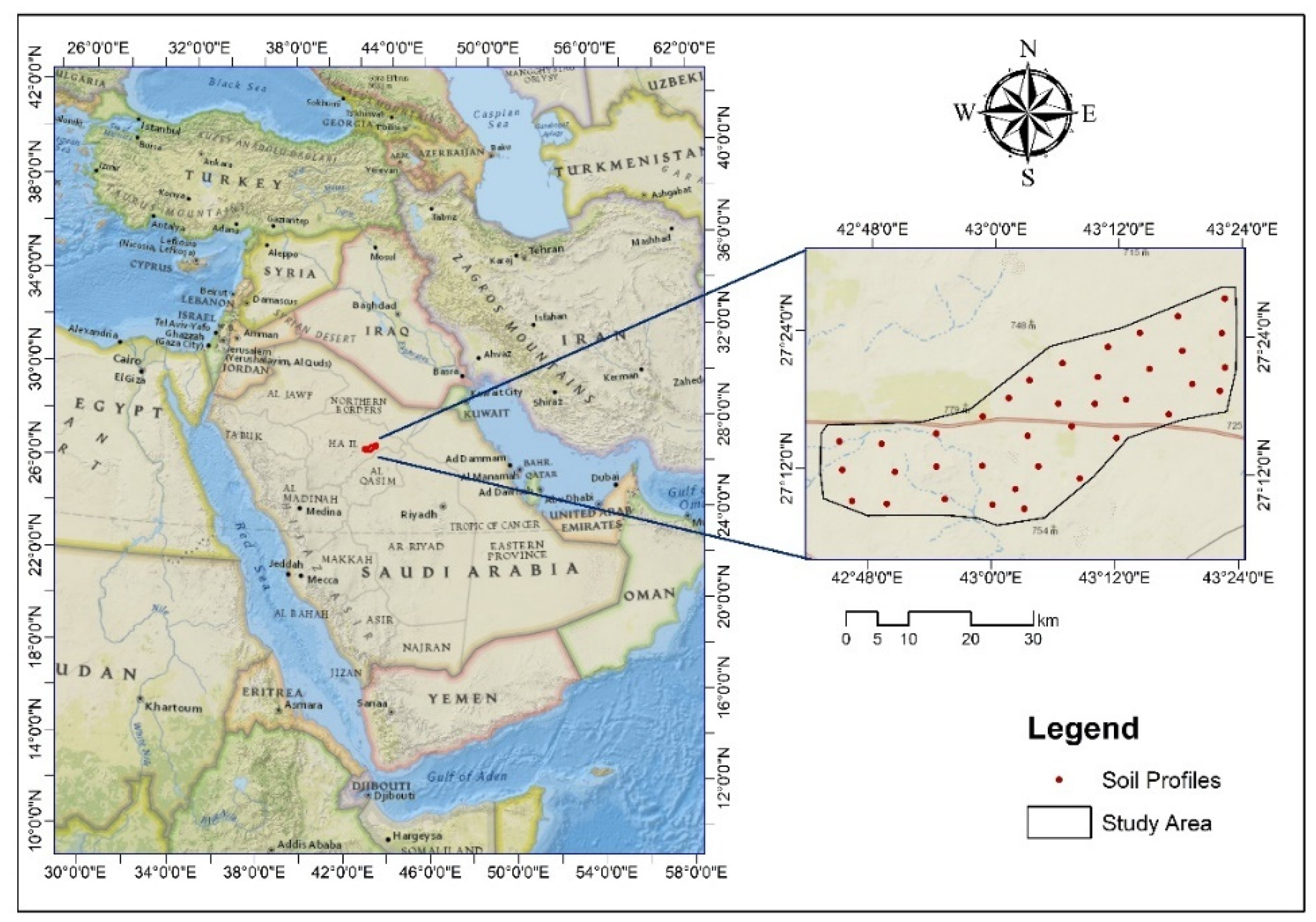
2.1. Study Area

This study was conducted in the Hail province in northwestern Saudi Arabia. The total studied area is about 1253.76 km2 and is located between latitudes 27°7′37.261″ and 27°27′45.367″ N and longitudes 42°42′56.441″ and 43°23′47.137″ E (Figure 1). Generally, the soils are characterized by sand to sandy loam texture with a deep profile [5]. The ground water is the main irrigation source in the area. There is no drainage network due to the use of the new irrigation techniques (Drip and Sprinkler irrigation). The climate in Hail is mild during summer with air temperatures ranging between 30 to 38 °C (The warmest month with the highest average high temperature is August (38 °C). At the same time, soil surface temperature fluctuated between 41 to 52 °C. While it is cold during winter with air temperatures between 3 to 15 °C and can drop to even 0 °C (The coldest month with the lowest average low temperature in January (3 °C)). Simultaneously, the temperature of the soil surface fluctuated from 22 to 25 °C and can drop to 6 °C in the coldest month. This period accompanied by rain and precipitation with total rainfall in the year is 186 mm. Air humidity throughout the year ranged between 18 to 55%. The average wind speed in Hail is mild seasonal variation over the year. The windier part of the year, from 19 October to 27 May, with average wind speeds of more than 14.16 km per hour. The calmer time of year is from 27 May to 19 October. The calmest month of the year is September, with an average hourly wind speed of 20.45 km h−1 [39]. Date palm, barley, alfalfa, wheat, maize, and a few vegetables are cultivated in some of the areas under investigation.

2.2. Fieldwork and Laboratory Analyses

The fieldwork aimed to characterize the soil properties by selecting sites according to surface soil characteristics. The total number of soil profiles was 37 in systematic depths (0–50, 50–100, and 100–150 cm) with 111 total soil samples. The soil profiles were located in UTM coordinate system by the GPS. The soil samples were air-dried and sieved through a 2 mm sieve to analyze the chemical, physical, and fertility characterization as follows:

2.2.1. Physical Properties

Soil particle size distribution was determined according to the hydrometer method [40]. Soil bulk density was determined from the volume-mass relationship for each core sample [41]. Saturated soil hydraulic conductivity was determined under a constant head [42]. Saturation percentage, field capacity, wilting point, and plant available water were determined using the method of [43].

2.2.2. Chemical Properties

Electrical conductivity (EC) was determined in the saturated soil paste extracted; soil reaction (pH) was determined in (1:2.5) soil water suspension [44]. Total calcium carbonate was determined volumetrically using Collin’s calcimeter [45]. Available nitrogen in the soil was extracted in the 2.0 M KCl and determined by micro-Kjeldahl apparatus. Available phosphorus was extracted in 0.5 N NaHCO3 solution (pH 8.5) and optical density was measured using a spectrophotometer. Available potassium was extracted in the 1.0 N ammonium acetate solution (pH 7) and measured using a flame photometer. Available N, P, and K were determined according to Page et al. [44]. Available Fe, Zn, Mn, and Cu were extracted by using DTPA and were assayed using an Inductively Coupled Plasma Atomic Emission Spectrometer (ICP-AES) (Thermo 7000) Thermo Scintific, Model iCAP7400 Duo [46].

2.2.3. Terrain Analysis

Was performed using Arc-GIS 10.8 software. Digital Elevation Model (DEM) derived using 38 × 38 m cell size thematic map. Slope and aspect were derived by spatial analyst extension using inverse distance weighting (IDW) interpolation techniques [47].

2.3. Statistical Analysis and Principal Component Analysis

Data were analyzed for descriptive measurements including minimum, maximum, arithmetic mean, median, range, variance, standard deviation, standard error, coefficient of variation, skewness, and kurtosis. The normality of variables was verified using the Shapiro-Wilk test before proceeding with the principal component analysis (PCA), and the correlation between different variables was measured by Pearson correlation. Furthermore, Bartlett’s sphericity test as well as Kaiser-Meyer-Olkin (KMO). The measure of Sampling Adequacy was conducted to verify data dependence, where if the KMO result is larger than 0.5 and the p-Value of Bartlett’s sphericity test is smaller than 0.05, this indicates the non-mutual independence of data and can be applied for PCA.
Soil properties were summarized using PCA. The PCA was performed using XLSTAT software version 2019.2.2.59614, Addinsoft, Boston, MA, USA [48]. PCA is a statistical procedure that uses an orthogonal transformation to convert a set of observations of possibly correlated variables (entities each of which takes on various numerical values) into a set of values of linearly uncorrelated variables called principal components (PCs). PCs having eigenvalues greater than one has been retained whereas PCs less than 1 were subtracted away [49].

2.4. Geostatistical Analysis

ArcGIS 10.8 software, 2019, Redlands, CA, USA was used to assess the spatial distribution pattern of different soil properties. Geostatistical and interpolation methods such as Ordinary Kriging was used to assess the spatial distribution of soil characteristics (Equation (1)) [50].
z ^ ( x 0 ) = i = 1 n λ i   z ( x i )
where z ^ ( x 0 ) is the value to be estimated at the location of x0, z(xi) is the known value at the sampling site xi and n is the number of sites surrounded by the search neighborhood used for the estimation.
The Semi-variogram models can be used with ordinary kriging (OK) for each soil property to represent the average rate of variation of soil property with distance. It is the basis for modeling the data set and for drawing a contour map [51].
The semi-variogram γ(h) is defined as:
γ ( h ) = 1 2 V a r [ Z ( x ) Z ( x + h ) ]  
where Z(x) and Z(x + h) are the values of a random function representing the soil property of interest z, at places x and x + h separated by the vector h known as the lag or interval.
The accomplished semi-variogram values for each lag were fitted to one of the semi-variogram models (i.e., Stable, J-Bessel, K-Bessel, Hole Effect, Rational Quadratic, Gaussian, Exponential, Pentaspherical, Tetraspherical, Spherical, and Circular) using Arc GIS 10.8, 2019, Redlands, CA, USA. The selected model was evaluated based on criteria where the best fit model which has a mean error “ME”, average standard error “ASE” and mean standardized error “MSE” values close to zero [52].

2.5. Site-Specific Management Zones

Agglomerative hierarchical clustering (AHC) was executed to define soil management zones. XLSTAT software version 2019.2.2.59614, Addinsoft, Boston, MA, USA was used to classify the data into different clusters having a common trait [48]. A one-way ANOVA test was performed for comparison between soil management zones and followed by a post hoc test using Duncan multiple range (DMR) test for comparisons between management zones.

3. Results and Discussion

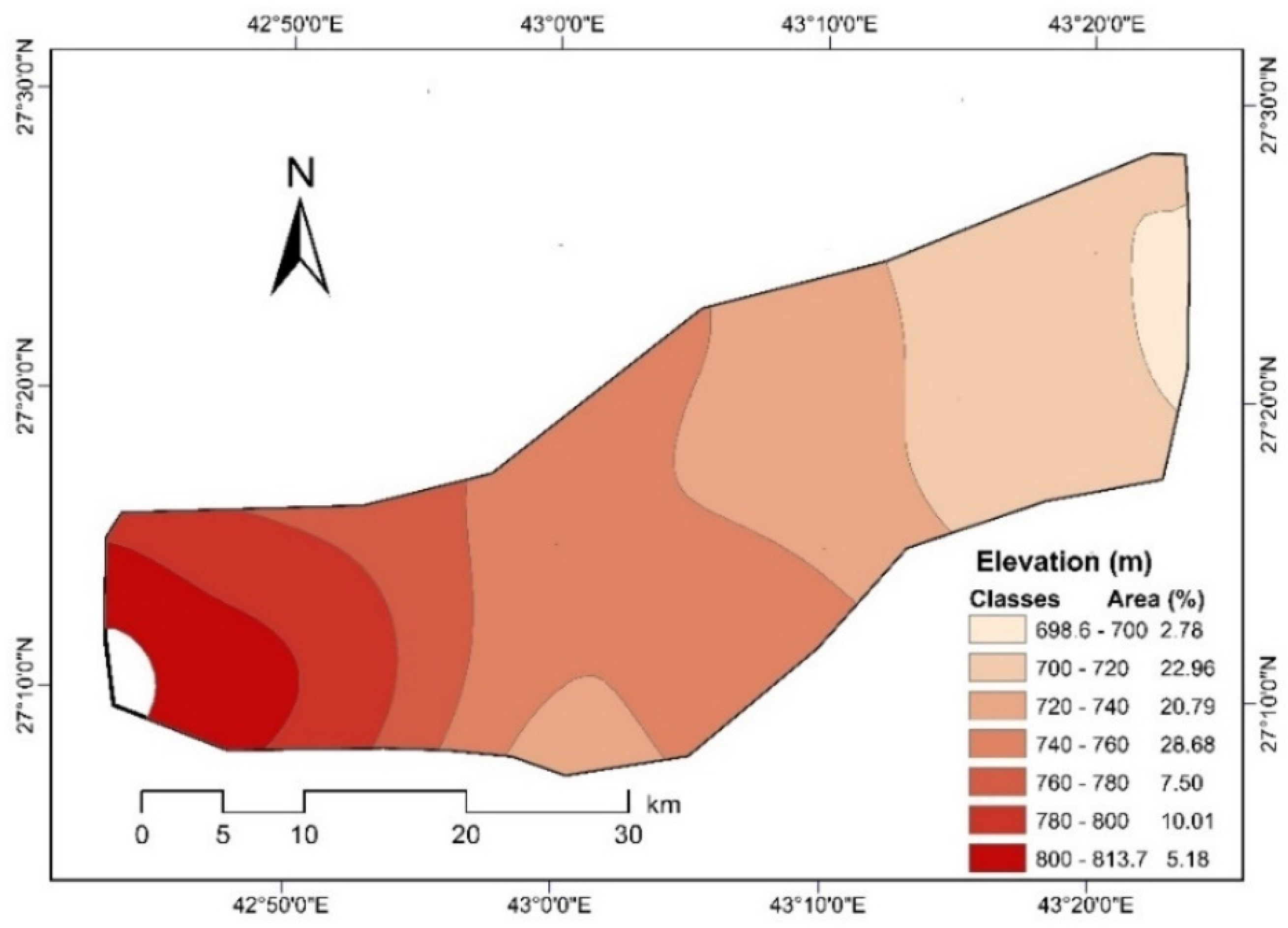
3.1. Terrain Analysis

Digital Elevation Model analysis (DEM) indicated that the elevations varied from 698.6 to 813.7 m A.S.L. The lowest elevation part of the study area was located in the eastern. The prevailing elevation ranged from 700 to 760 m A.S.L. comprised 72.43% of the total area as shown in Figure 2. Soil surface slope is most important in terms of its effect on erosion. The soil depth increases with decreasing slope rate and decreases as the slope increases [53]. Using the Digital Elevation Model with GIS software gave the slope information data. The slope of the area ranged from 0 to 64.23% and the main slope class was from 0 to 9.57% which covered about 77.19% (96,777.42 ha) of the total area. This slope can classify as slightly inclined (Table 1). The slope indirectly restricts agricultural production by affecting soil properties negatively. It is noticeable that the directions of the area under investigation are in equal percentages in all direction classes as shown in Table 1, Alharbi and Aggag [54].

3.2. Statistical Characterization of the Studied Soil

The soil is characterized as sand to sandy loam deep soil with low fertility content and low water holding capacity. Table 2 shows the descriptive statistical analysis which indicated that a wide variation in soil EC, pH, CaCO3, available N, P, K, micronutrients Fe, Zn, Mn, Cu, and soil physical properties Sand, Clay, BD, SP, PWP, AW and Ks were recorded (Table 2). The distribution of variation in soil properties over space was highly skewed for all the properties except available phosphorus and B.D. Kurtosis in soil properties was also found to behave similarly.
Among soil properties, maximum variability was recorded for EC (1.04–18.94 dSm−1) with mean, CV%, skewness, and kurtosis being 4.69, 93.4, 1.82, and 3.11, respectively (Figure 3b, Table 2). Higher EC was observed in the higher altitudes in the western area as reported by Alharbi and Aggag [54]. The soil pH was in the acidic range (7.52–8.24) with mean, standard deviation, and CV% being 7.92, 0.20, and 2.4, respectively (Table 2). The lower CV in pH is explained to be due to uniform conditions in the study area as indicated by the least skewness (−0.41). The alkaline reaction of soil is attributed to the alkaline parent material, climate, topography, and precipitation. Similar results have been reported in the area of Hail, KSA by Alharbi and Aggag [54]. CaCO3 showed wide variability (0.9–17.2%) with the mean and CV being 6.4% and 61.6% (Figure 3m, Table 2). The clay content ranged from 10.0 to 25.9% with mean and standard deviation being 17.1% and 3.7. Abdel-Fattah [38] stated that the study area is categorized as moderate to high salinity soils, with ECe values varying from 0.87 to 20.33 dSm−1 with an average value of 5.30 ± 5.05 dSm−1.
Wide variations in DTPA Fe, Zn, Mn, and Cu were recorded with respective mean values of 674.6, 235.2, 536.7, and 145.3 µg kg−1 (Table 2). This indicated a widespread deficiency of micronutrients in the area under investigation. The four micronutrients CV, ranging from 47.4 to 96.7 show high variability. The highest CV was observed for Fe (96.7%) followed by Cu (87.2%), Mn (53.8%), and Zn (47.4%). The spatial prevalence of four micronutrients reflected similar trends in skewness and kurtosis values ranging from 1.32 to 4.21 and 2.17 to 21.72, respectively (Table 2). The Kolmogorov-Smirnov and the Shapiro-Wilk Tests result showed that the soil properties (ECe, K, Fe, Zn, Mn, Cu, sand, clay, SP, FC, PWP, AW, and Ks) are not normally distributed (p-Values < 0.05). Therefore, the data were transformed using the logarithmic transformation method before assuming the spatial distribution of soil properties using the ordinary kriging (OK) method [55]. While, pH, CaCO3, available N, P, and BD are normally distributed (Table 2). Amer [56] found that all soil properties do not follow a normal distribution, where the value of p of the Shapiro-Wilk Test is less than 0.05 except for the CEC property. Furthermore, Gozukara [57] discovered that the EC, SOM, CaCO3, P, Zn, and Mn were not distributed normally. The parameters were then logarithmically transformed to achieve a normal distribution.

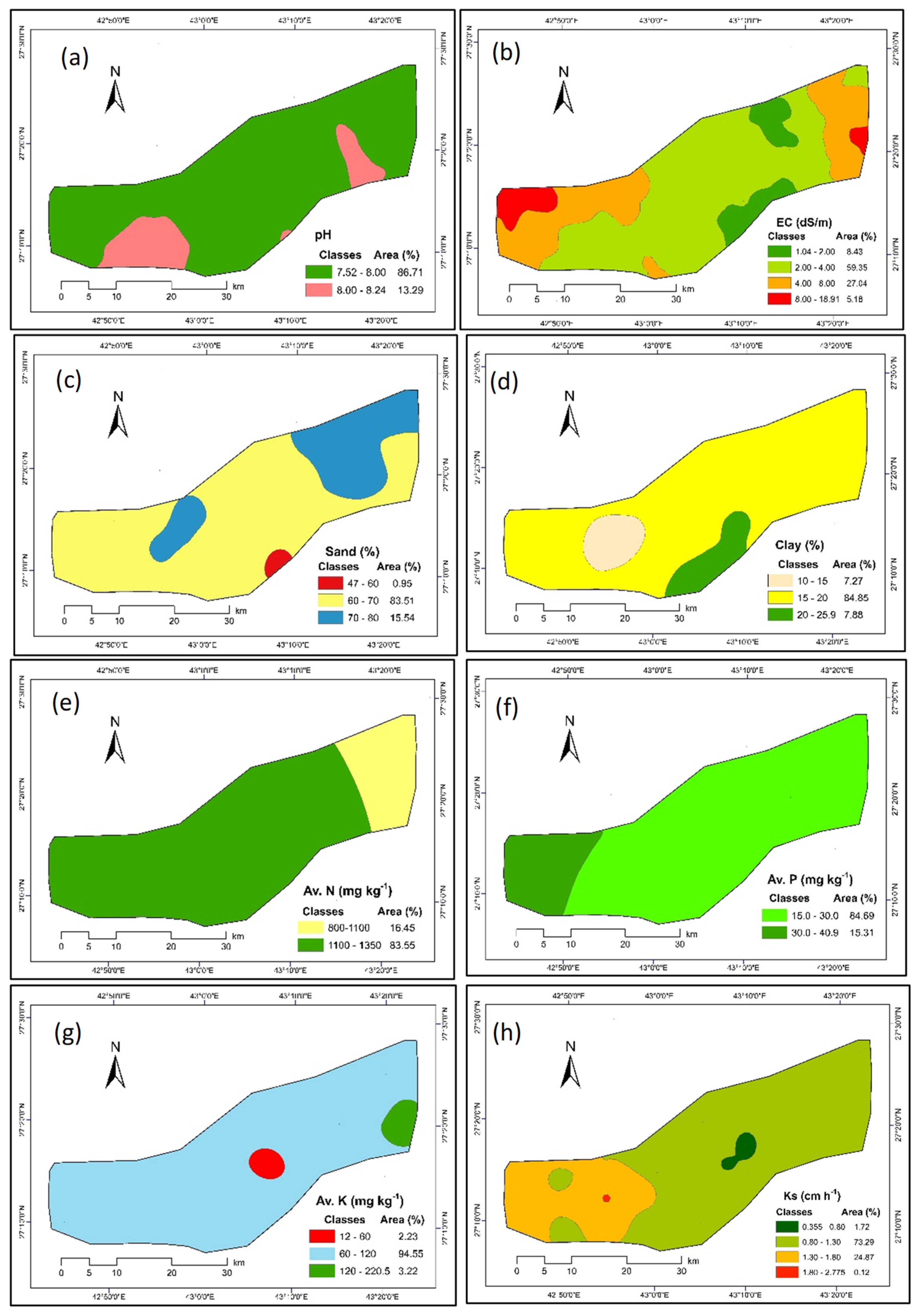
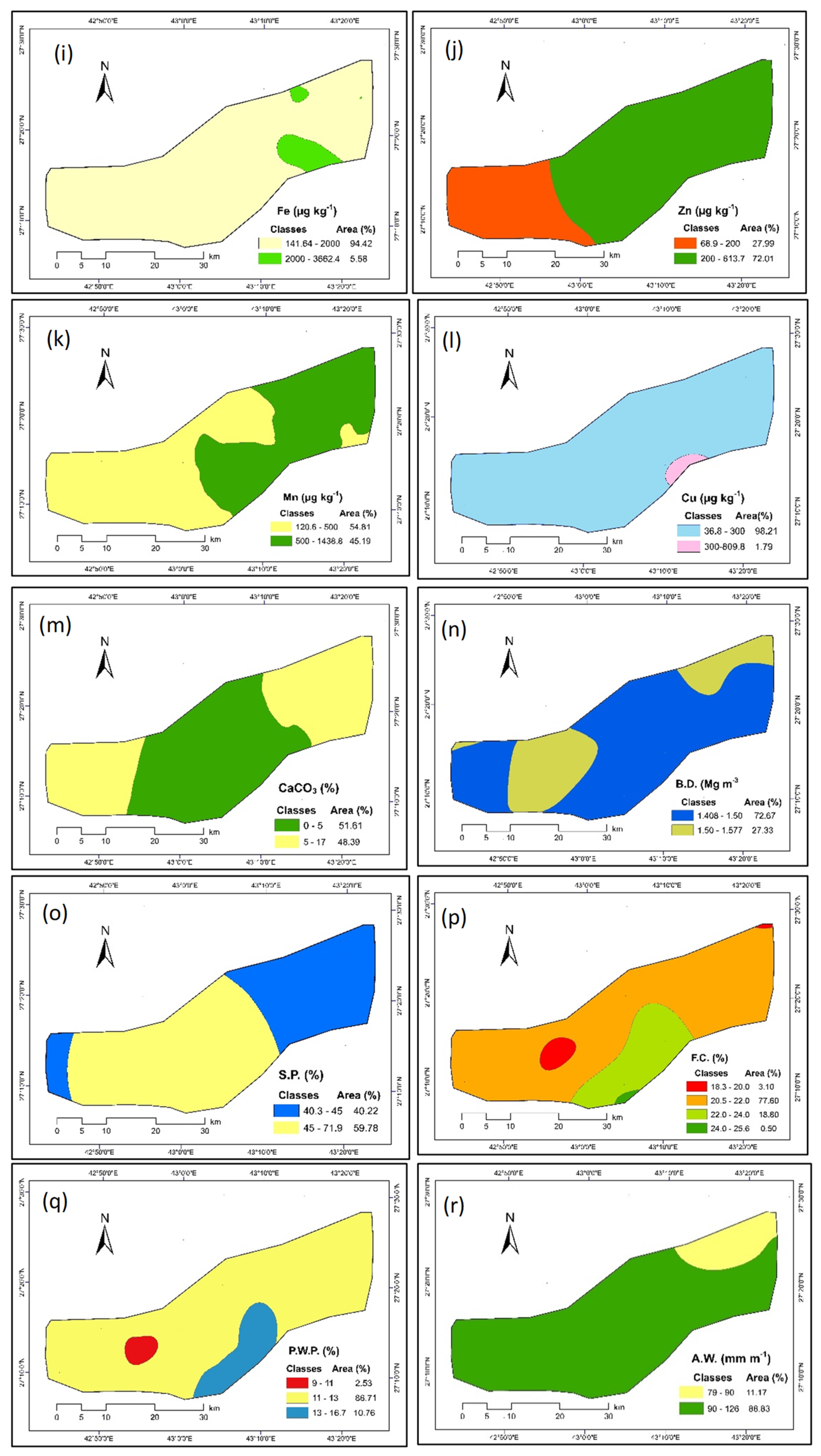
3.3. Distribution of Soil Properties

The measured salinity value ranged between 1.09 to 18.94 dSm−1, indicating low, medium to high soil salinity as recorded by Richard [58]. About 8.43% (10,569.15 ha) of the study area has low salinity and is well suitable for agriculture, 59.35% (10,569.16 ha) area shows medium salinity, and 32.22% (40,395.98 ha) of the area show high salinity (Figure 3b). About 86.71% of the area (108,713.09 ha) has a pH between 7.52 to 8.00 (slightly alkaline), and 13.29% (16,662.40 ha) has a pH between 8.00 and 8.24 (alkaline) (Figure 3a) [59]. The CaCO3% in the study area ranged between 0.9 and 17.2% and classified into low, (less than 5%) at about 51.61% of the area (64,706.30 ha), and medium (5 to 17%) 48.39% (60,669.20 ha) (Figure 3m). Most of the area is classified as medium nitrogen content (1000–1350 ppm) which covers 98.73% of the area (123,783.23 ha) and 1.27% of the area (1592.27 ha) classified as low N content (less than 1000 ppm) according to classification by Barthakur and Baruah [59]. Whereas 94.55% of the area (118,542.53 ha) was classified as medium potassium concentration (60–120 ppm K), 3.22% of the area (4037.09 ha) was classified as high K-concentration (greater than 120 ppm), and 2.23% of the area (2795.87 ha) has low K-concentration (less than 60 ppm). While 84.69% of the area (106,180.51 ha) was classified as medium phosphorus concentration (15–30 ppm P), and 15.31% of the area (19,182.45 ha) has high P-concentration (30–40.9 ppm), as classified by Barthakur and Baruah [59]. The investigated area has low micronutrients Fe, Zn, Mn, and Cu concentrations (Figure 3i–l); less than 4000, 600, 2000, and 200 µg/kg, respectively as mentioned by Reddy [60]. The available N ranges between 1.33 mg kg−1 and 61.6 mg kg−1, indicating that the nitrogen content in the area is low. The available P content ranges from low 2.33 mg kg−1 to high 19.84 mg kg−1, and available K ranges from 32.76 mg kg−1 to 734 mg kg−1, which is classified as high [37]. Zn, Cu, Fe, and Mn levels varied greatly, with mean values of 0.28, 0.44, 8.51, and 8.59 mg kg−1. Verma et al. [37] stated that micronutrient distribution varies due to parent material, climatic conditions, and anthropogenic activities.
The clay fraction range of less than 20% is classified as low and covers 92.12% (115,495.91 ha) of the study area and medium categories 20 to 26% clay covering 7.88% (9879.59 ha) of the study area (Figure 3d). Most of the area 72.67% (91,110.37 ha) has B.D. between 1.41 to 1.50 Mg m−3 and 27.33% (34,265.12 ha) have B.D. between 1.50 to 1.58 Mg m−3 (Figure 3n). The greatest of the area 96.89% (121476.32 ha) has medium FC between 20 to 25.6% and 3.11% (3899.17 ha) has less than 20% of FC (Figure 3p). A major of the area, 88.83% (111371.05 ha), has medium AW between 90 to 126 mm m−1 and 11.17% (14004.44 ha) has low AW, less than 90 mm m−1 (Figure 3r). These results were in agreement with those found by Brady et al. [61] and Abdel-Fattah [38].

3.4. Relationships between Soil Properties

A Pearson correlation test was running out to study the relationship between different soil properties as presented in Table 3. Some of the soil properties had significant correlations with each other. EC had a negative correlation with soil pH at P = 0.05 level. N and P were negatively correlated with Fe at P = 0.05. Whereas a positive correlation was found between each EC and K, N and P, and between Zn and Cu [62]. It was observed that there were positive strong significant correlations between clay and FC, and PWP while negative correlations were with BD and Ks. Correspondingly, negative correlation between sand and clay, FC, PWP, and AW; while positive correlation with BD.
Using a biplot (Figure 3), where the angles between the vectors show how traits correlate with one another, we can corroborate this from these correlations between the various variables. Variables have a positive correlation when they are near together and create a small angle. They are not likely to be associated if they intersect at a 90° angle. They are negatively correlated when they diverge and produce a significant angle that is nearly 180 degrees. Consequently, one or more major general components of these variables are present. According to the correlation between various soil properties, principal components analysis (PCA) was used to determine the principal sources of data variability. This is also supported by Bartlett’s sphericity and KMO tests (Table 4), where small p-Values (p < 0.05) of the significance level indicate that a PCA may be useful with these data [63]. Table 3 contains the results of Bartlett’s sphericity test. The observed p-Value is less than 0.001. Because the KMO values were greater than 0.586, a PCA may be useful for these data [64,65].

3.5. Geostatistical Analysis and Spatial Variability

The semivariogram-derived best-fit models for various soil parameters were presented in Table 5. Additionally, Figure 3 shows the spatial maps of soil properties. The best fit models were J-Bessel (pH, Clay, BD, and AW), K-Bessel for (EC and Av. N), Stable (CaCO3, P, K, Fe, Zn, Sand, FC, and Ks), Spherical (Mn and Cu), Gaussian (SP), exponential (PWP). Gozukara et al. [25] reported that the exponential semivariogram model had the lowest prediction error with the lowest RMSE for sand and silt content on the soil surface, whereas the spherical semivariogram model had the lowest prediction error with the lowest RMSE. Similar best-fit models for various soil properties have also been reported by [66,67]. The models for the soil properties at various sites show how anthropogenic activities and the local environment have an impact on the spatial variability of soil properties.
The nugget is the measurement of the errors that sampling, measurement technique, and other sources contribute to overall variation. It denotes microvariability, and its values for various soil characteristics ranged from 0 to 50.72; the lowest values were for EC, FC, and BD, and the highest was for P, with the exception of Fe, which was extremely high and reached 14515.83. The nugget values of all the studied parameters were very small and varied from 0 to 1.23 [56]. Large nugget values indicated that ecological practices were affecting soil indicators on a small scale, and the chosen sampling distance could not adequately capture the spatial dependence [68].
Sill is theoretically equal to the variance of the sampled population at a large separation distance if the data has no trend [69]. The highest sill was recorded for N (14598.83) followed by P (78.65) whereas BD, sand, FC, AW, PWP, SP, pH, and clay has the lowest recorded 0.0, 0.01, 0.01, 0.01, 0.02, 0.02 followed by 0.04 and 0.05, respectively. The sill ratio for remaining soil properties varied between 0.23 and 15.07.
If the value of the nugget-to-sill ratio was <0.25, 0.25–0.75, and >0.75, this exposes strong (attributable to intrinsic factors), moderate (attributable to both intrinsic and extrinsic factors) and weak (attributable to extrinsic factors) spatial dependence, respectively [70]. The nugget: sill ratio, which indicates the relationship between location and ratio, showed that the soil’s EC, Cu, and Ks characteristics were strong, while pH, P, K, Fe, Mn, sand, clay, BD, SP, FC, and PWP were moderate and CaCO3, N, Zn, and AW were weak (Table 4). Nugget-to-sill ratio values were less than 0.25 for all the studied soil properties except CEC [56].
Spatially dependent soil attributes are affected by parent material inherent to the soil, mineralogy, texture, farming techniques, and other anthropogenic activities. Variations in terrain, fertilizer application rates, nutrient management techniques, and diverse flora all affect how location and soil properties interact in different ways. The underlying mineralogy and parent material are ascribed to the high geographical dependency of soil characteristics [37]. Extrinsic factors such as soil management including tillage and fertilizer application influence moderate and weak spatial dependence of soil properties [24].
The semivariogram’s range value can be interpreted as the farthest distance at which there is spatial dependency or autocorrelation. The range of soil property values was 11.08 for manganese to 46.97 km for nitrogen (Table 5). Beyond this point, autocorrelation is absent. Large-range values show that measured soil properties are impacted by natural and human-made causes over a wider area [24]. Kerry and Oliver [71] state that the delay between soil samples should be no more than half the semivariogram range value.
Kriged maps of pH, ECe, CaCO3, available macro and micronutrients, and hydrological properties were created by ordinary kriging interpolation methods to evaluate the distribution of these nutrients (Figure 3a–r) which were successfully applied by many studies [72]. Future studies will use these maps as a knowledge resource. The maps can be used by individual farmers to adopt a variable rate of nutrient application in certain places. The maps will also serve as a foundation of knowledge for State authorities, decision-makers, and extension specialists as they build site-specific strategies for landscape management and application of balanced nutrients. Applications for computers and mobile devices that are based on these maps will provide farmers with more exact and balanced rates of nutrient application [37].

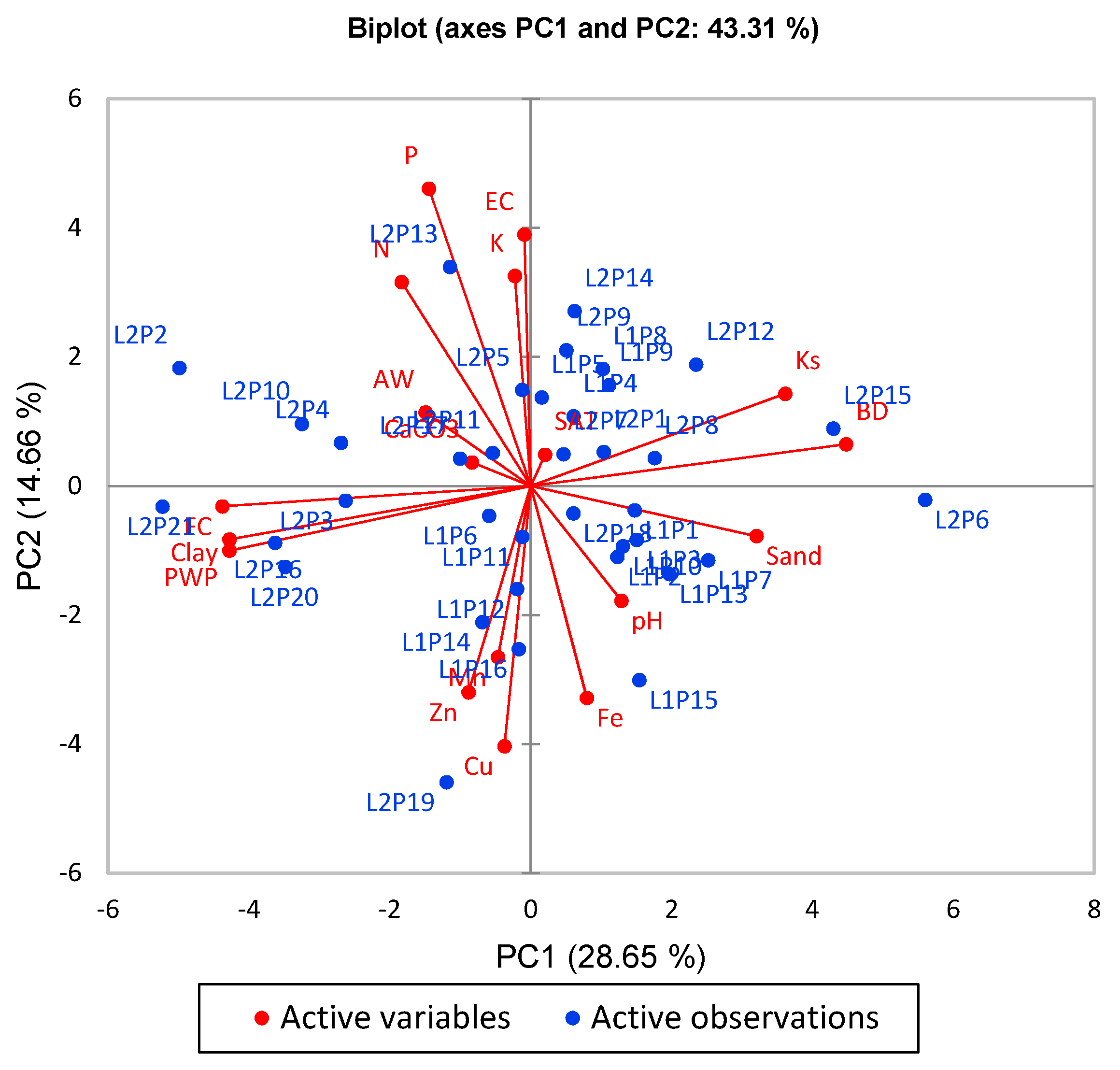
3.6. Principle Components Analysis (PCA)

The principal component analysis (PCs) was used to sort through major soil properties to determine which can contribute the most to soil quality improvement and help priorities immediate management action. PCs with eigenvalues greater than or equal to 1.0 were chosen for this purpose; therefore, these PCs were used according to the method described by Kaiser [73] while PCs with eigenvalues less than 1 were subtracted. As a result, the first six PCs had eigenvalues greater or equal to 1.0 and a cumulative variability of 79.75%. (Table 6 and Figure 4). PC1, 2, 3, 4, 5, and 6 contributed 28.6%, 14.7%, 12.5%, 10.4%, 7.6%, and 5.9%, respectively. BD dominated the PC1 loading, followed by FC, clay, PWP, Ks, and sand. PC2 was dominated by N, ECe, and CaCO3; PC3 was dominated by pH; PC4 was dominated primarily by K and P, PC5 was mainly dominated by Fe; Mn, and Cu, and PC6 was mainly dominated by SP and Zn. A biplot chart depicts the graphical representation of the variability contribution by PC1 and PC2, as well as the loadings for different soil properties (Figure 4). This will aid in decision making regarding the identification of properties for prioritization of physical, chemical, and nutrient management strategies in this area under investigation to improve agriculture production and reduce the effects of land degradation. Soil status of BD, FC, PWP, Ks, N, ECe, and CaCO3 matters in that order may be used as criteria to decide priorities for improving water and salt and nutrient content based on variable loading of soil properties in different PCs and expert opinion.

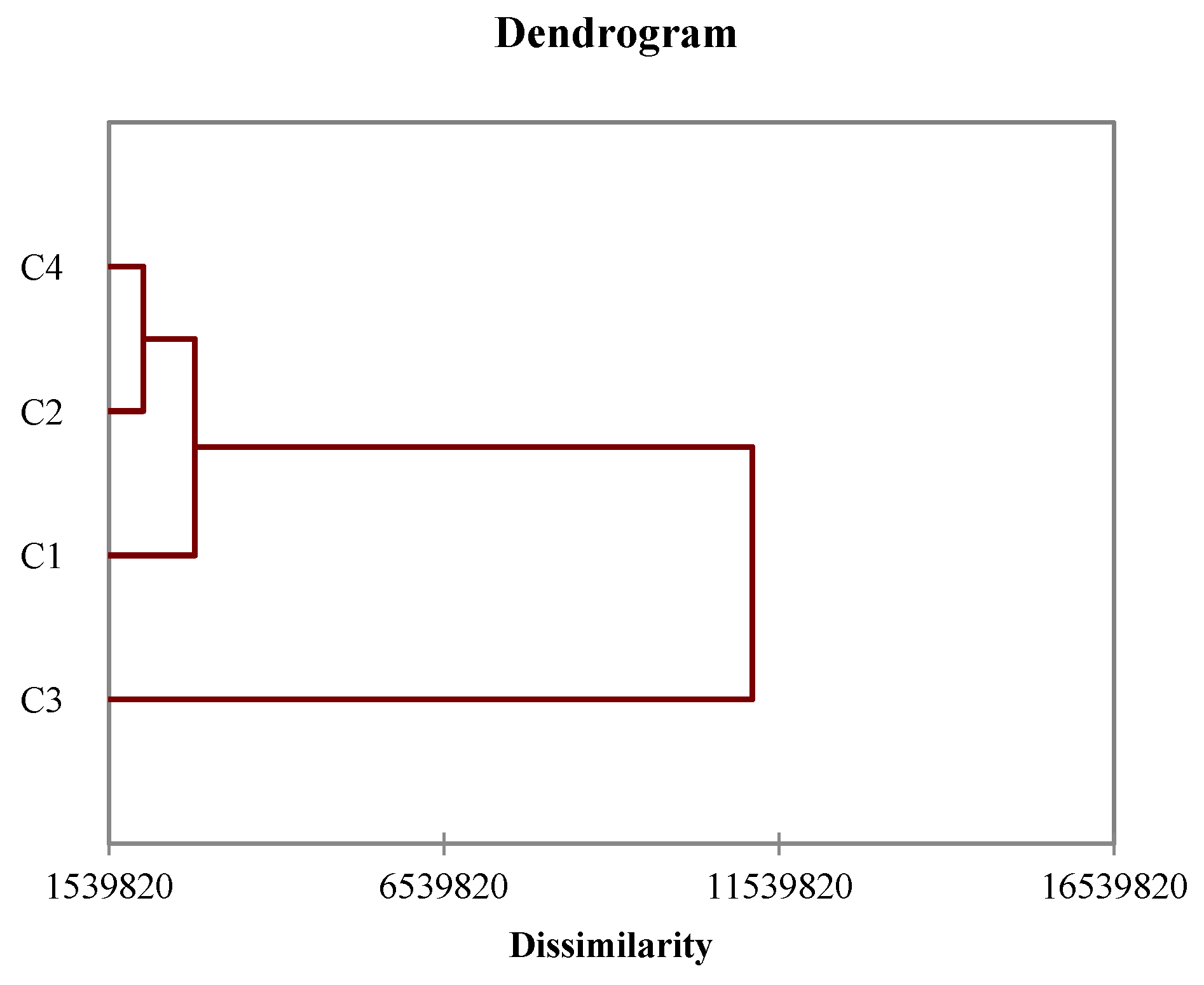
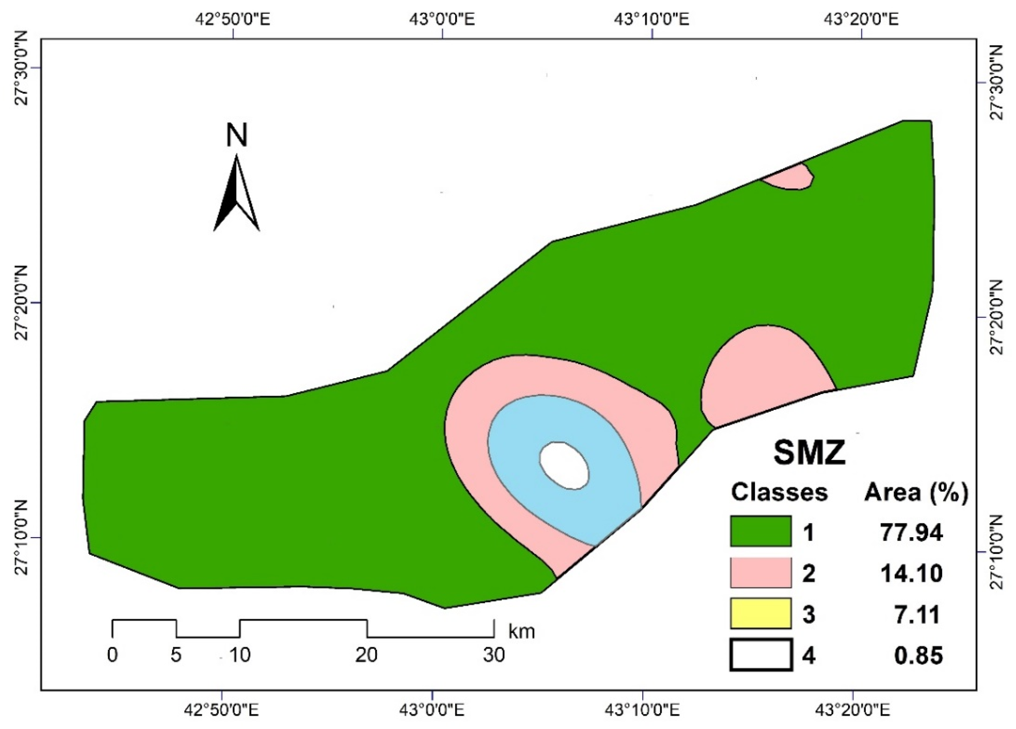
3.7. Initiating Management Zones Using Soil Properties

A cluster analysis was applied to classify the four PCs into MZs. The XLSTAT was used based on the AHC technique to define the optimum number of MZs. This method allows us to differentiate different zones with a similar value of properties and higher differences between them [74]. To obtain the optimum number of MZs and plotted as shown in Figure 5, against the number of clusters (or MZs). In this study, four different management zones were finally identified as the optimum number of MZs, as shown in Figure 5. The four SMZs were distinctly different from each other and the percent areas were 77.94, 14.10, 7.11, and 0.85% for SMZ1, SMZ2, SMZ3, and SMZ4 respectively. Figure 6 shows the spatial distribution map of the four delineated MZs in the study area. In each delineated MZ, the measured soil properties present the lowest variance and highest degree of membership. Thus, in each zone, different management practices, such as agriculture management can be carried out to increase crop production while decreasing costs. Therefore, the one-way ANOVA was carried out to evaluate the effectiveness of the PCA and AHP combination to delineate MZs and also its spatial variability. There were significant differences (p < 0.05) between all soil and terrain attributes except for N, Zn, AW, and Ks among the four MZs, as shown in Table 7. The MZ1 and MZ3 which covers 85.05% of the area under investigation had a mean value of ECe as 3.03 and 4.52 dSm−1 and were classified as moderately salinized soils, greater than the limiting critical value for the sensitive crops. Whereas the MZ2 which covers 14.10% of the area has 7.23 dSm−1 of ECe and must be leached to remove salts from the soil and reduce ECe to less than 2 dSm−1 to get high productivity. When the total amount of salts accumulated in the root zone is high enough, negatively affects plant growth by reducing the plant’s available water [75]. Only 0.85% of the area has low ECe, as shown in Table 7. In all MZs, the soil available nitrogen, zinc, available water content, and saturated hydraulic conductivity remains tight and did not show significant differences. The four MZs have low clay, available N, P, and lower micronutrient concentrations. Thus, these MZs have a great potential for environmental risk via nitrogen leaching through the soil profiles and also nitrogen load in soil surface run-off, especially with a high percentage of sand. This finding is diagnostic for determining the amount of fertilizer and irrigation water to be applied to soils in different management zones. Its emphasis’s the importance of site-specific management for long-term crop productivity and, as a result, reducing environmental hazards caused by uneven fertilizers application. Moreover, all of the delineated MZs had low hydrological properties (SP, FC, PWP, and AW) and should be taken into account in agriculture management processes. According to several studies, analysis of variance is an effective method for determining the differences between delineation zones. [74,76,77,78].

4. Conclusions

A total of 111 soil samples were collected from 37 soil profiles in systematic depths (0–50, 50–100, and 100–150 cm) from the South Hail region, KSA. The samples were analyzed for pH, ECe, CaCO3, and accessible macro and micronutrients and hydrological properties. A strong significant correlation was observed between most of the soil properties. The best fit models were J-Bessel for pH, Clay, BD, and AW; K-Bessel for EC and Av. N; Stable for CaCO3, P, K, Fe, Zn, Sand, FC, and Ks; Spherical for Mn and Cu; Gaussian for SP; whereas exponential for PWP. The PCA resulted in six principal components (PCs) explaining 79.75% of the total variance of soil properties. The PC1 was strongly influenced by soil BD, FC, clay, PWP, Ks, and sand. PC2 was dominated by N, ECe, and CaCO3; PC3 was dominated by pH; PC4 was dominated primarily by K and P, PC5 was mainly dominated by Fe; Mn, and Cu, and PC6 was mainly dominated by SP and Zn. Based on agglomerative hierarchical clustering, four soil management zones (MZs) cover 77.94, 14.10, 7.11 and 0.85% of studied area. MZ 1 and 3 classified as moderately saline while MZ 2 classified as highly saline soils. This area must be leached to remove salts and reduce ECe to less than 2 dSm−1, to get maximum productivity. All MZs have a great potential for environmental risk via nutrients leaching through the soil profiles, especially with a high percentage of sand. This finding is diagnostic for determining the amount of fertilizer and irrigation water to be applied to soils in different management zones. Moreover, all of the delineated MZs had low hydrological properties (SP, FC, PWP, and AW) and should be taken into account in agriculture management processes.

Author Contributions

Conceptualization, A.M.A. and A.A.; methodology, A.A.; software, A.M.A.; validation, A.M.A. and A.A.; formal analysis, A.M.A.; resources, A.A.; writing—original draft preparation, A.M.A. and A.A.; visualization, A.M.A. All authors have read and agreed to the published version of the manuscript.

Funding

This research received no external funding.

Institutional Review Board Statement

Not applicable.

Informed Consent Statement

Not applicable.

Data Availability Statement

Not applicable.

Acknowledgments

The researchers would like to thank the Deanship of Scientific Research, Qassim University for funding the publication of this project.

Conflicts of Interest

The authors declare no conflict of interest.

References

  1. Bremer, E.; Ellert, K. Soil Quality Indicators: A Review with Implications for Agricultural Ecosystems in Alberta; AESA: Lethbridge, AB, Canada, 2004. [Google Scholar]
  2. Statistics, H. Agricultural Production Survey Bulletin; General Authority for Statistics: Riyadh, Saudi Arabia, 2019. [Google Scholar]
  3. Modaihsh, A.S.; Sallam, A.S.; Ghoneim, A.M.; Mahjoub, M.O. Assessing salt-affected degraded soils using remote sensing. Case study: Al-Qassim region, Saudi Arabia. J. Food Agric. Environ. 2014, 12, 383–388. [Google Scholar]
  4. Abdel-Satar, A.M.; Al-Khabbas, M.H.; Alahmad, W.R.; Yousef, W.M.; Alsomadi, R.H.; Iqbal, T. Quality assessment of groundwater and agricultural soil in Hail region, Saudi Arabia. Egypt. J. Aquat. Res. 2017, 43, 55–64. [Google Scholar] [CrossRef]
  5. Alharbi, A.; Abd-Elmoniem, E.; Asiry, K.A. Correlation of Soil Salinity with the Physico-chemical Properties of Agricultural Soils from the Hail Region of Saudi Arabia. Cienc. Tec. 2017, 2, 2–24. [Google Scholar]
  6. Elaalem, M.M. Spatial Variability of Some Soil Chemical Proprieties in Jeffara Plain, Libya (Case Study: Tripoli, Wadi Almjainin and Bin Ghashir). Libyan J. Agric. 2017, 22, 19–34. [Google Scholar]
  7. Bekele, A.; Hudnall, W.H. Spatial variability of soil chemical properties of a prairie–forest transition in Louisiana. Plant Soil 2006, 280, 7–21. [Google Scholar] [CrossRef]
  8. Cruz, J.S.; de Assis Júnior, R.N.; Matias, S.; Tamayo, J.H.C. Spatial variability of an Alfisol cultivated with sugarcane. Cienc. Investig. Agrar. Rev. Latinoam. Cienc. Agric. 2011, 38, 155–164. [Google Scholar]
  9. Jabro, J.; Stevens, W.; Evans, R.; Iversen, W. Spatial variability and correlation of selected soil properties in the Ap horizon of a CRP grassland. Appl. Eng. Agric. 2010, 26, 419–428. [Google Scholar] [CrossRef] [Green Version]
  10. Fraisse, C.; Sudduth, K.; Kitchen, N.; Fridgen, J. Use of Unsupervised Clustering Algorithms for Delineating within-Field Management Zones; American Society of Agricultural Engineers: St. Joseph, MI, USA, 1999. [Google Scholar]
  11. Aggag, A.; Yehia, H. GIS mapping of land suitability and soil quality for some soils of El-Sharkeya Governorate, Egypt. J. Agric. Env. Sci. 2006, 5, 40–64. [Google Scholar]
  12. Bodaghabadi, M.B.; Martínez-Casasnovas, J.; Khakili, P.; Masihabadi, M.; Gandomkar, A. Assessment of the FAO traditional land evaluation methods, a case study: Iranian land classification method. Soil Use Manag. 2015, 3, 384–396. [Google Scholar] [CrossRef] [Green Version]
  13. Camacho-Tamayo, J.H.; Luengas, C.A.; Leiva, F.R. Effect of agricultural intervention on the spatial variability of some soils chemical properties in the eastern plains of Colombia. Chil. J. Agric. Res. 2008, 68, 42–55. [Google Scholar] [CrossRef]
  14. El Baroudy, A.A. Mapping and evaluating land suitability using a GIS-based model. Catena 2016, 140, 96–104. [Google Scholar] [CrossRef]
  15. Jimoh, A.I.; Yusuf, Y.O.; Yau, S.L. Soil suitability evaluation for rain-fed maize production at Gabari District Zaria Kaduna State, Nigeria. Ethiop. J. Environ. Stud. Manag. 2016, 9, 137–147. [Google Scholar] [CrossRef] [Green Version]
  16. Santra, P.; Chopra, U.; Chakraborty, D. Spatial variability of soil properties and its application in predicting surface map of hydraulic parameters in an agricultural farm. Curr. Sci. 2008, 95, 937–945. [Google Scholar]
  17. Malczewski, J. GIS-based multicriteria decision analysis: A survey of the literature. Int. J. Geogr. Inf. Sci. 2006, 20, 703–726. [Google Scholar] [CrossRef]
  18. Vasu, D.; Singh, S.; Sahu, N.; Tiwary, P.; Chandran, P.; Duraisami, V.; Ramamurthy, V.; Lalitha, M.; Kalaiselvi, B. Assessment of spatial variability of soil properties using geospatial techniques for farm level nutrient management. Soil Tillage Res. 2017, 169, 25–34. [Google Scholar] [CrossRef]
  19. Kazemi, H.; Sadeghi, S.; Akinci, H. Developing a land evaluation model for faba bean cultivation using geographic information system and multi-criteria analysis (A case study: Gonbad-Kavous region, Iran). Ecol. Indic. 2016, 63, 37–47. [Google Scholar] [CrossRef]
  20. Gupta, A.; Kamble, T.; Machiwal, D. Comparison of ordinary and Bayesian kriging techniques in depicting rainfall variability in arid and semi-arid regions of north-west India. Environ. Earth Sci. 2017, 76, 512. [Google Scholar] [CrossRef]
  21. Li, L.; Zhao, J.; Yuan, T. Study on Approaches of Land Suitability Evaluation for Crop Production Using GIS; Springer: Berlin/Heidelberg, Germany, 2011; pp. 587–596. [Google Scholar]
  22. Webster, R.; Oliver, M. Geostatistics for Experimental Scientists; John Wiley and Sons Ltd.: Chichester, UK, 2001. [Google Scholar]
  23. Al-Omran, A.M.; Aly, A.A.; Al-Wabel, M.I.; Al-Shayaa, M.S.; Sallam, A.S.; Nadeem, M.E. Geostatistical methods in evaluating spatial variability of groundwater quality in Al-Kharj Region, Saudi Arabia. Appl. Water Sci. 2017, 7, 4013–4023. [Google Scholar] [CrossRef] [Green Version]
  24. Behera, S.K.; Mathur, R.K.; Shukla, A.K.; Suresh, K.; Prakash, C. Spatial variability of soil properties and delineation of soil management zones of oil palm plantations grown in a hot and humid tropical region of southern India. Catena 2018, 165, 251–259. [Google Scholar] [CrossRef]
  25. Gozukara, G.; Akça, E.; Dengiz, O.; Kapur, S.; Adak, A. Soil particle size prediction using Vis-NIR and pXRF spectra in a semiarid agricultural ecosystem in Central Anatolia of Türkiye. Catena 2022, 217, 106514. [Google Scholar] [CrossRef]
  26. Gozukara, G. Rapid land use prediction via portable X-ray fluorescence (pXRF) data on the dried lakebed of Avlan Lake in Turkey. Geoderma Reg. 2022, 28, e00464. [Google Scholar] [CrossRef]
  27. Hastie, T.; Tibshirani, R.; Friedman, J. The Elements of Statistical Learning: Data Mining, Inference, and Prediction; Springer Series in Statistics; Springer: New York, NY, USA, 2009. [Google Scholar] [CrossRef]
  28. Yuan, Y.; Miao, Y.; Yuan, F.; Ata-UI-Karim, S.T.; Liu, X.; Tian, Y.; Zhu, Y.; Cao, W.; Cao, Q. Delineating soil nutrient management zones based on optimal sampling interval in medium-and small-scale intensive farming systems. Precis. Agric. 2022, 23, 538–558. [Google Scholar] [CrossRef]
  29. Boroushaki, S.; Malczewski, J. Implementing an extension of the analytical hierarchy process using ordered weighted averaging operators with fuzzy quantifiers in ArcGIS. Comput. Geosci. 2008, 34, 399–410. [Google Scholar] [CrossRef]
  30. Romano, G.; Dal Sasso, P.; Trisorio Liuzzi, G.; Gentile, F. Multi-criteria decision analysis for land suitability mapping in a rural area of Southern Italy. Land Use Policy 2015, 48, 131–143. [Google Scholar] [CrossRef]
  31. Chen, J. GIS-based multi-criteria analysis for land use suitability assessment in City of Regina. Environ. Syst. Res. 2014, 1, 13. [Google Scholar] [CrossRef]
  32. Gong, J.; Liu, Y.; Chen, W. Land suitability evaluation for development using a matter-element model: A case study in Zengcheng, Guangzhou, China. Land Use Policy 2012, 29, 464–472. [Google Scholar] [CrossRef]
  33. Seyedmohammadi, J.; Sarmadian, F.; Jafarzadeh, A.A.; McDowell, R.W. Development of a model using matter element, AHP and GIS techniques to assess the suitability of land for agriculture. Geoderma 2019, 352, 80–95. [Google Scholar] [CrossRef]
  34. Brevik, E.C.; Calzolari, C.; Miller, B.A.; Pereira, P.; Kabala, C.; Baumgarten, A.; Jordán, A. Soil mapping, classification, and pedologic modeling: History and future directions. Geoderma 2016, 264, 256–274. [Google Scholar] [CrossRef]
  35. Moharana, P.; Jena, R.; Pradhan, U.; Nogiya, M.; Tailor, B.; Singh, R.; Singh, S. Geostatistical and fuzzy clustering approach for delineation of site-specific management zones and yield-limiting factors in irrigated hot arid environment of India. Precis. Agric. 2020, 21, 426–448. [Google Scholar] [CrossRef]
  36. Saito, H.; McKenna, S.A.; Zimmerman, D.; Coburn, T.C. Geostatistical interpolation of object counts collected from multiple strip transects: Ordinary kriging versus finite domain kriging. Stoch. Environ. Res. Risk Assess. 2005, 19, 71–85. [Google Scholar] [CrossRef]
  37. Verma, R.R.; Manjunath, B.L.; Singh, N.P.; Kumar, A.; Asolkar, T.; Chavan, V.; Srivastava, T.K.; Singh, P. Soil mapping and delineation of management zones in the Western Ghats of coastal India. Land Degrad. Dev. 2018, 29, 4313–4322. [Google Scholar] [CrossRef]
  38. Abdel-Fattah, M.K. A GIS-based approach to identify the spatial variability of salt affected soil properties and delineation of site-specific management zones: A case study from Egypt. Soil Sci. Annu. 2020, 71, 76–85. [Google Scholar] [CrossRef]
  39. Weather Spark. Available online: https://weatherspark.com/y/101927/Average-Weather-in-Ha'il-Saudi-Arabia-Year-Round (accessed on 18 July 2022).
  40. Gee, G.W.; Bauder, J.W. Particle-size analysis. In Methods of Soil Analysis, Part 1-Physical Mineralogical Methods; Klute, A., Ed.; American Society of Agronomy: Madison, WI, USA, 1986; pp. 383–399. [Google Scholar]
  41. Blake, G.R.; Hartge, K.H. Bulk Density. In Methods of Soil Analysis, Part 1-Physical Mineralogical Methods; Klute, A., Ed.; American Society of Agronomy: Madison, WI, USA, 1986; pp. 363–375. [Google Scholar]
  42. Klute, A.; Dirksen, C. Hydraulic conductivity and diffusivity: Laboratory methods. In Methods of Soil Analysis: Part 1-Physical Mineralogical Methods; American Society of Agronomy: Madison, WI, USA, 1986; pp. 687–734. [Google Scholar]
  43. Cassel, D.; Nielsen, D. Field capacity and available water capacity. In Methods of Soil Analysis: Part 1-Physical Mineralogical Methods; American Society of Agronomy: Madison, WI, USA, 1986; pp. 901–926. [Google Scholar]
  44. Page, A.; Miller, R.; Keeney, D. Methods of Soil Analysis. Part 2. Chemical and Microbiological Properties; Agronomy, No. 9; American Society of Agronomy: Madison, WI, USA, 1982. [Google Scholar]
  45. Loeppert, R.; Suarez, D. Carbonate and gypsum. In Methods of Soil Analysis. Part 3. Chemical Methods; Sparks, D., Page, A.L., Helmke, P.A., Loeppert, R.H., Soltanpour, P.N., Tabatabai, M.A., Johnston, C.T., Sumner, M.E., Eds.; SSSA Book Series 5; SSSA: Madison, WI, USA, 1996; pp. 437–474. [Google Scholar]
  46. Soltanpour, P.; Schwab, A. A new soil test for simultaneous extraction of macro-and micro-nutrients in alkaline soils. Commun. Soil Sci. Plant Anal. 1977, 8, 195–207. [Google Scholar] [CrossRef]
  47. ESRI. ArcGIS, version 10.8; ESRI: Redlands, CA, USA, 2019.
  48. Addinsoft. XLSTAT; Statistical and data analysis solution; Addinsoft: Boston, MA, USA, 2019. [Google Scholar]
  49. Abdi, H.; Williams, L.J. Principal component analysis. Wiley Interdiscip. Rev. Comput. Stat. 2010, 2, 433–459. [Google Scholar] [CrossRef]
  50. Goovaerts, P. Geostatistical tools for characterizing the spatial variability of microbiological and physico-chemical soil properties. Biol. Fertil. Soils 1998, 27, 315–334. [Google Scholar] [CrossRef]
  51. Burgess, T.M.; Webster, R. Optimal interpolation and isarithmic mapping of soil properties. J. Soil Sci. 1980, 31, 315–331. [Google Scholar] [CrossRef]
  52. Gundogdu, K.S.; Guney, I. Spatial analyses of groundwater levels using universal kriging. J. Earth Syst. Sci. 2007, 116, 49–55. [Google Scholar] [CrossRef] [Green Version]
  53. Ennaji, W.; Barakat, A.; El Baghdadi, M.; Oumenskou, H.; Aadraoui, M.; Karroum, L.A.; Hilali, A. GIS-based multi-criteria land suitability analysis for sustainable agriculture in the northeast area of Tadla plain (Morocco). J. Earth Syst. Sci. 2018, 127, 79. [Google Scholar] [CrossRef] [Green Version]
  54. Alharbi, A.B.; Aggag, A. Land Evaluation for Alternative Crops of Alfalfa Using GIS in south Hail, Saudi Arabia. Alex. Sci. Exch. J. 2020, 41, 419–433. [Google Scholar] [CrossRef]
  55. Feng, C.; Hongyue, W.; Lu, N.; Chen, T.; He, H.; Lu, Y.; Tu, X. Log-transformation and its implications for data analysis. Shanghai Arch. Psychiatry 2014, 26, 105–109. [Google Scholar] [CrossRef]
  56. Amer, B.S.; Moussa, K.F.; Sheha, A.A.; Abdel-Fattah, M.K. Delineation of site-specific management zones using multivariate analysis and geographic information system technique. Plant Arch. 2021, 21, 1385–1390. [Google Scholar] [CrossRef]
  57. Gozukara, G.; Acar, M.; Ozlu, E.; Dengiz, O.; Hartemink, A.E.; Zhang, Y. A soil quality index using Vis-NIR and pXRF spectra of a soil profile. Catena 2022, 211, 105954. [Google Scholar] [CrossRef]
  58. Richards, L. Diagnosis and Improvement of Saline Alkali Soils; Handbook; Williams & Wilkins: Philadelphia, PA, USA, 1954; Volume 60. [Google Scholar] [CrossRef]
  59. Barthakur, H.; Baruah, T. Text Book of Soil Analysis; Vikas Publishing House (Pvt) Ltd.: New Delhi, India, 1997. [Google Scholar]
  60. Reddy, D.T.P. Critical levels of micro and secondary nutrients in soils and crops for optimum plant nutrition. Int. J. Sci. Res. 2021, 6, 594–595. [Google Scholar]
  61. Brady, N.C.; Weil, R.R.; Weil, R.R. The Nature and Properties of Soils; Prentice Hall: Upper Saddle River, NJ, USA, 2008; Volume 13. [Google Scholar]
  62. Patel, K.S.; Chikhlekar, S.; Ramteke, S.; Sahu, B.L.; Dahariya, N.S.; Sharma, R. Micronutrient status in soil of Central India. Am. J. Plant Sci. 2015, 6, 3025. [Google Scholar] [CrossRef] [Green Version]
  63. Sofroniou, N.; Hutcheson, G.D. The Multivariate Social Scientist; Sage Publications: Thousand Oaks, CA, USA, 1999; pp. 1–288. [Google Scholar]
  64. Huck, S.W.; Cormier, W.H.; Bounds, W.G. Reading Statistics and Research; Pearson: Boston, MA, USA, 1974. [Google Scholar]
  65. Tabachnick, B.G.; Fidell, L.S.; Ullman, J.B. Using Multivariate Statistics; Pearson: Boston, MA, USA, 2007; Volume 5. [Google Scholar]
  66. Behera, S.K.; Shukla, A.K. Spatial distribution of surface soil acidity, electrical conductivity, soil organic carbon content and exchangeable potassium, calcium and magnesium in some cropped acid soils of India. Land Degrad. Dev. 2015, 26, 71–79. [Google Scholar] [CrossRef]
  67. Mali, S.; Naik, S.; Bhatt, B. Spatial variability in soil properties of mango orchards in eastern plateau and hill region of India. Vegetos 2016, 29, 74–79. [Google Scholar] [CrossRef]
  68. Zhang, X.-Y.; Yue-Yu, S.; Zhang, X.-D.; Kai, M.; Herbert, S. Spatial variability of nutrient properties in black soil of northeast China. Pedosphere 2007, 17, 19–29. [Google Scholar] [CrossRef]
  69. Mulla, D. Modeling and mapping soil spatial and temporal variability. In Hydropedology; Elsevier: Amsterdam, The Netherlands, 2012; pp. 637–664. [Google Scholar]
  70. Cambardella, C.A.; Moorman, T.B.; Novak, J.; Parkin, T.; Karlen, D.; Turco, R.; Konopka, A. Field-scale variability of soil properties in central Iowa soils. Soil Sci. Soc. Am. J. 1994, 58, 1501–1511. [Google Scholar] [CrossRef]
  71. Kerry, R.; Oliver, M. Average variograms to guide soil sampling. Int. J. Appl. Earth Obs. Geoinf. 2004, 5, 307–325. [Google Scholar] [CrossRef]
  72. Ozlu, E.; Gozukara, G.; Acar, M.; Bilen, S.; Babur, E. Field-Scale Evaluation of the Soil Quality Index as Influenced by Dairy Manure and Inorganic Fertilizers. Sustainability 2022, 14, 7593. [Google Scholar] [CrossRef]
  73. Kaiser, H.F. The application of electronic computers to factor analysis. Educ. Psychol. Meas. 1960, 20, 141–151. [Google Scholar] [CrossRef]
  74. Oldoni, H.; Terra, V.S.S.; Timm, L.C.; Júnior, C.R.; Monteiro, A.B. Delineation of management zones in a peach orchard using multivariate and geostatistical analyses. Soil Tillage Res. 2019, 191, 1–10. [Google Scholar] [CrossRef]
  75. Warrence, N.J.; Bauder, J.W.; Pearson, K.E. Basics of Salinity and Sodicity Effects on Soil Physical Properties; Departement of Land Resources and Environmental Sciences, Montana State University: Bozeman, MT, USA, 2002; Volume 129, pp. 1–29. [Google Scholar]
  76. Abdel-Fattah, M.K.; Mohamed, E.S.; Wagdi, E.M.; Shahin, S.A.; Aldosari, A.A.; Lasaponara, R.; Alnaimy, M.A. Quantitative evaluation of soil quality using Principal Component Analysis: The case study of El-Fayoum depression Egypt. Sustainability 2021, 13, 1824. [Google Scholar] [CrossRef]
  77. Rahul, T.; Kumar, N.A.; Biswaranjan, D.; Mohammad, S.; Banwari, L.; Priyanka, G.; Sangita, M.; Bihari, P.B.; Narayan, S.R.; Kumar, S.A. Assessing soil spatial variability and delineating site-specific management zones for a coastal saline land in eastern India. Arch. Agron. Soil Sci. 2019, 65, 1775–1787. [Google Scholar] [CrossRef]
  78. Wang, X.-Z.; Liu, G.-S.; Hu, H.-C.; Wang, Z.-H.; Liu, Q.-H.; Liu, X.-F.; Hao, W.-H.; Li, Y.-T. Determination of management zones for a tobacco field based on soil fertility. Comput. Electron. Agric. 2009, 65, 168–175. [Google Scholar]
Figure 1. Location of the study area with sampling positions.
Sustainability 14 16209 g001
Figure 2. Digital Elevation Model for the area under study.
Sustainability 14 16209 g002
Figure 3. Spatial distribution (kriged) maps of soil pH (a), EC (b), Sand (c), clay (d), N (e), P (f), K (g), and Ks (h) in south Hail, KSA. Spatial distribution (kriged) maps of soil Fe (i), Zn (j), Mn (k), Cu (l), CaCO3 (m), B.D. (n), S.P. (o), F.C. (p), P.W.P. (q), and A.W. (r) in south Hail, KSA.
Sustainability 14 16209 g003aSustainability 14 16209 g003b
Figure 4. PCA biplot (PC1 vs. PC2) of soil properties in South Hail located in KSA.
Sustainability 14 16209 g004
Figure 5. Dendrogram for Agglomerative hierarchical clustering.
Sustainability 14 16209 g005
Figure 6. Management zones (MZs) kriged map of South Hail located in KSA.
Sustainability 14 16209 g006
Table 1. Area percentage of DEM, slope, and direction classes for the study area.
Digital Elevation Model (DEM)Slope ClassesDirection Classes
Elevation Range, mArea, %Slope Class, %Area, %Direction ClassArea, %
698.6–7002.780–3.7825.26Flat1.55
700–72022.963.79–6.5528.96North11.16
720–74020.796.56–9.5722.97North East13.02
740–76028.689.58–13.1013.33East12.92
760–7807.5013.11–17.636.39South East12.48
780–80010.0217.64–24.942.58South12.62
800–813.77.2724.95–64.230.51South West12.20
West12.14
North West11.91
Table 2. Statistical characterization of soil properties.
ParameterMin.Max.MeanVarianceStd. Dev.CVSkewnessKurtosisNormality Test
Shapiro-Walk TestKolmogorov-Smirnov Test
WSig.Dsig.
ECe (dSm−1)1.0418.914.6919.134.3893.381.823.110.77<0.00010.240.024
pH (1:2.5 soil: water)7.528.247.920.040.202.42−0.41−0.580.960.250.080.940
CaCO3 (%)0.8517.236.3515.273.9161.620.740.280.940.060.100.831
Av. N (mg kg−1)800.01350.01135.114,564.6120.710.63−0.47−0.030.940.050.160.245
Av. P (mg kg−1)8.0040.9022.9685.519.2540.280.22−0.640.950.120.110.773
Av. K (mg kg−1)12.00220.5100.73574.759.7959.400.50−0.930.930.020.160.289
DTPA Fe (µg kg−1)141.643662.4674.6425,894.4652.6196.743.2012.410.65<0.00010.260.010
DTPA Zn (µg kg−1)68.85613.7235.212,422.5111.4647.401.322.900.910.010.140.386
DTPA Mn (µg kg−1)120.601438.8536.783,336.9288.6953.791.332.170.900.000.160.248
DTPA Cu (µg kg−1)36.84809.8145.316,048.8126.6987.204.2121.720.57<0.00010.200.101
Sand (%)47.0080.0068.0847.016.8610.07−1.162.010.920.010.140.433
Clay (%)10.0025.9017.1113.683.7021.620.780.720.960.020.160.269
B.D. (Mg m−3)1.411.581.490.000.042.39−0.140.680.400.200.140.407
S.P. (%)40.3071.9044.7522.894.7910.695.3330.810.92<0.00010.310.001
F.C. (%) 18.3025.6021.383.331.838.530.860.260.940.010.140.441
P.W.P. (%)9.0016.7012.042.401.5512.870.891.600.930.040.150.312
A.W. (mm m−1)80.00126.0093.3099.449.9810.691.532.810.850.000.240.022
Ks (cm h−1)0.362.781.120.240.4943.881.413.050.900.000.200.097
Note. AW: available water; BD: bulk density; DTPA: diethylene-triamine-penta-acetic acid; EC: electrical conductivity; F.C.: field capacity; Ks: saturated hydraulic conductivity; PWP: permanent wilting point; S.P.: saturation percentage.
Table 3. Matrix of Pearson’s correlation coefficients between the soil properties used in this study.
VariablesECpHNPKFeZnMnCuCaCO3SandClayBDSPFCPWPAWKs
ECe (dSm−1)1
pH (1:2.5 soil: water)−0.536 *1
Av. N (mg kg−1)0.033−0.2291
Av. P (mg kg−1)0.273−0.1560.528 *1
Av. K (mg kg−1)0.716 *−0.3100.0330.2171
DTPA Fe (µg kg−1)0.0070.094−0.434 *−0.556 *0.1741
DTPA Zn (µg kg−1)−0.084−0.243−0.131−0.175−0.0020.1871
DTPA Mn (µg kg−1)−0.1540.0950.016−0.228−0.1700.2960.1031
DTPA Cu (µg kg−1)−0.1400.015−0.267−0.236−0.2180.1840.596 *0.1491
CaCO3 (%)0.178−0.137−0.0230.0260.2200.223−0.0520.059−0.0901
Sand (%)−0.090−0.098−0.205−0.273−0.0380.094−0.013−0.144−0.004−0.0581
Clay (%)−0.131−0.2690.3680.189−0.043−0.1280.1720.0660.1160.113−0.441 *1
B.D. (Mg m−3)0.0290.193−0.261−0.181−0.0540.078−0.164−0.074−0.098−0.1610.657 *−0.895 *1
S.P. (%)−0.0710.071−0.1200.074−0.030−0.123−0.006−0.081−0.030−0.080−0.107−0.0320.0541
F.C. (%) −0.023−0.0960.2740.215−0.012−0.0920.1350.1200.0720.101−0.832 *0.837 *−0.915 *0.0161
P.W.P. (%)−0.112−0.3000.2650.136−0.055−0.1290.1880.0530.0680.175−0.448 *0.948 *−0.914 *−0.0370.833 *1
A.W. (mm m−1)0.1190.2320.1260.2130.052−0.0220.0080.1260.0090.001−0.836 *0.082−0.2630.1390.544 *0.0101
Ks (cm h−1)0.0250.321−0.135−0.092−0.0660.008−0.239−0.115−0.144−0.2410.232−0.779 *0.815 *0.192−0.606 *−0.836 *0.2071
Note. AW: available water; BD: bulk density; CaCO3: calcium carbonate; DTPA: diethylene-triamine-penta-acetic acid; EC: electrical conductivity; F.C.: field capacity; Ks: saturated hydraulic conductivity; PWP: permanent wilting point; S.P.: saturation percentage. * Correlation is significant at a probability level of 0.05.
Table 4. Bartlett’s Sphericity Test and KMO Measure of Sampling Adequacy.
KMO Measure of Sampling Adequacy0.586
Bartlett’s Sphericity Test
Chi-square (Observed value)568.457
Chi-square (Critical value)196.609
DF153
p-Value<0.0001
alpha0.01
Table 5. Semivariogram parameters of soil properties for the area under investigation.
VariablesModelNuggetPartial SillSillNugget/SillRange (m)MSE
ECe (dSm−1)K-Bessel0.000.6810.680.0021,238.424.399
pHJ-Bessel0.030.0120.040.6817,359.250.196
CaCO3 (%)Stable15.070.015.071.0017,472.564.036
Av. N (mg kg−1)K-Bessel14,515.8383.00014,598.830.9946,971.71122.565
Av. P (mg kg−1)Stable50.7227.93478.650.6417,359.258.231
Av. K (mg kg−1)Stable0.400.1430.540.7433,708.1284.609
DTPA Fe (µg kg−1)Stable0.190.2640.450.4115,044.21541.570
DTPA Zn (µg kg−1)Stable0.200.0330.230.8626,154.06126.429
DTPA Mn (µg kg−1)Spherical0.220.0850.300.7211,080.77367.920
DTPA Cu (µg kg−1)Spherical0.080.3550.430.1815,340.7387.910
Sand (%)Stable0.010.0070.010.4837,650.316.847
Clay (%)J-Bessel0.030.020.050.6720,425.333.748
B.D. (Mg m−3)J-Bessel0.000.000.000.5721,798.390.034
S.P. (%)Gaussian0.010.000.020.4423,877.114.131
F.C. (%)Stable0.000.000.010.5316,586.411.650
P.W.P. (%)Exponential0.010.010.020.5920,963.861.559
A.W. (mm m−1)J-Bessel0.010.010.010.7939,149.099.221
Ks (cm h−1)Stable0.000.210.210.0020,827.910.532
Note. AW: available water; BD: bulk density; DTPA: diethylene-triamine-penta-acetic acid; EC: electrical conductivity; F.C.: field capacity; Ks: saturated hydraulic conductivity PWP: permanent wilting point; S.P.: saturation percentage.
Table 6. Principal component analysis of soil properties and loading coefficient for first six principal components.
PC1PC2PC3PC4PC5PC6
Eigenvalue5.1572.6392.2481.8761.3671.069
Variability (%)28.64814.66112.48810.4237.5955.936
Cumulative (%)28.64843.30955.79766.22073.81579.751
PC loading for each variable
PC1PC2PC3PC4PC5PC6
ECe (dSm−1)−0.0190.601−0.4780.4920.162−0.065
pH0.277−0.2750.6850.047−0.2810.110
CaCO3 (%)−0.3950.4870.118−0.349−0.026−0.465
Av. N (mg kg−1)−0.3120.7110.135−0.1650.194−0.115
Av. P (mg kg−1)−0.0490.502−0.4980.5030.0200.080
Av. K (mg kg−1)0.172−0.506−0.2770.564−0.2960.018
DTPA Fe (µg kg−1)−0.191−0.493−0.2730.1380.622−0.148
DTPA Zn (µg kg−1)−0.100−0.4090.1140.233−0.274−0.510
DTPA Mn (µg kg−1)−0.081−0.622−0.0880.1170.553−0.145
DTPA Cu (µg kg−1)−0.1800.056−0.3430.290−0.4690.154
Sand (%)0.690−0.120−0.498−0.453−0.0360.019
Clay (%)−0.922−0.128−0.086−0.209−0.0370.070
B.D. (Mg m−3)0.9650.1000.021−0.0190.065−0.100
S.P. (%)0.0440.0750.3060.0610.3160.656
F.C. (%) −0.943−0.0490.2240.168−0.0130.047
P.W.P. (%)−0.922−0.155−0.147−0.206−0.0810.149
A.W. (mm m−1)−0.3220.1760.6310.6160.130−0.123
Ks (cm h−1)0.7790.2210.4030.1900.133−0.068
Note. AW: available water; BD: bulk density; DTPA: diethylene-triamine-penta-acetic acid; EC: electrical conductivity; F.C.: field capacity; Ks: saturated hydraulic conductivity; PWP: permanent wilting point; S.P.: saturation percentage.
Table 7. Mean values of soil properties in different management zones of South Hail located in KSA.
MZNo.ECpHNPKFeZnMnCuCaCO3SandClayBDS.P.F.C.P.W.PA.W.Ks
1244.52 ab7.91 b1147.9 a25.5 a98.7 ab432.4 b233.5 bc367.5 c135.1 b5.9 b68.8 ab16.9 b1.49 a45.1 a21.2 b12.0 b92.6 bc1.17 a
277.23 a7.89 c1078.6 ab15.9 bc120.1 a1069.1 ab244.1 ab707.8 b157.7 ab7.9 a67.2 b15.9 b1.49 a43.7 b21.1 b11.6 b94.4 ab1.11 ab
323.03 b8.02 a1000.0 bc8.1 c140.3 a2953.0 a257.0 a764.7 ab216.2 a8.7 a71.1 a17.5 b1.49 a44.0 b21.3 b12.0 b89.5 c0.98 bc
442.03 c7.95 ab1225.0 c27.3 a58.6 b297.8 b218.4 c1138.1 a149.1 b4.9 b63.7 c20.2 a1.47 b45.0 a22.8 a13.1 a97.3 a0.85 c
Note. AW: available water; BD: bulk density; DTPA: diethylene-triamine-penta-acetic acid; EC: electrical conductivity; F.C.: field capacity; Ks: saturated hydraulic conductivity; No: number of profiles; PWP: permanent wilting point; S.P.: saturation percentage; a,b,c: Values not sharing similar letters are significantly differenct (p > 0.05).
Publisher’s Note: MDPI stays neutral with regard to jurisdictional claims in published maps and institutional affiliations.

