
The Potential of UAV Imagery for the Detection of Rapid Permafrost Degradation: Assessing the Impacts on Critical Arctic Infrastructure


Abstract
1. Introduction
2. Materials and Methods
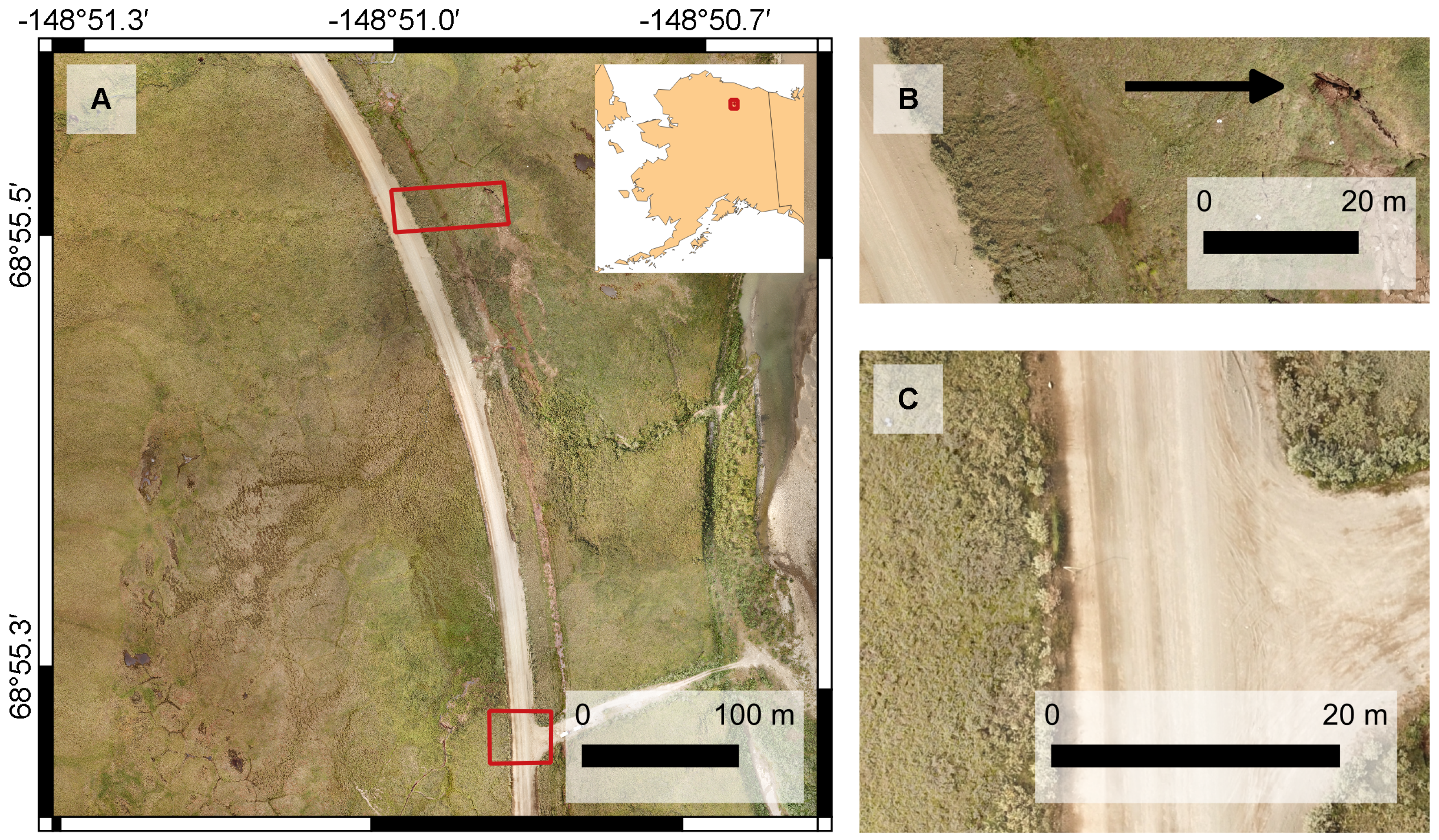
2.1. Study Area
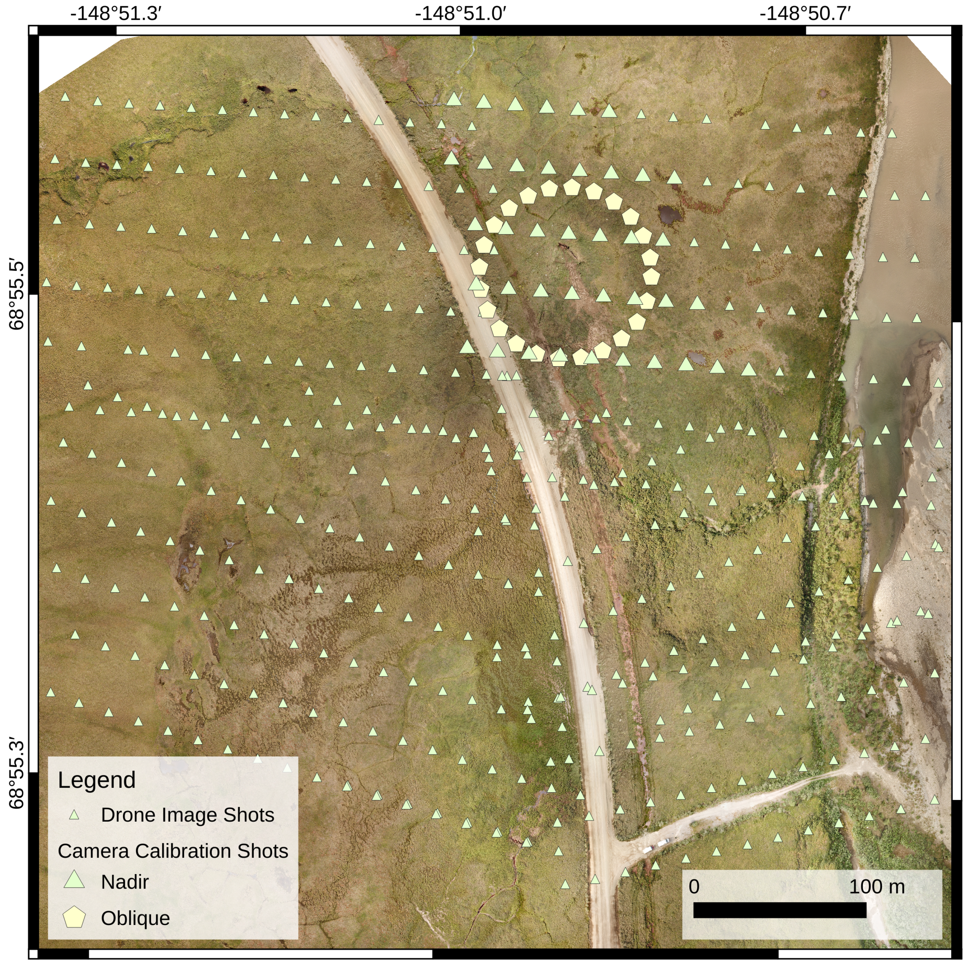
2.2. Image Acquisition
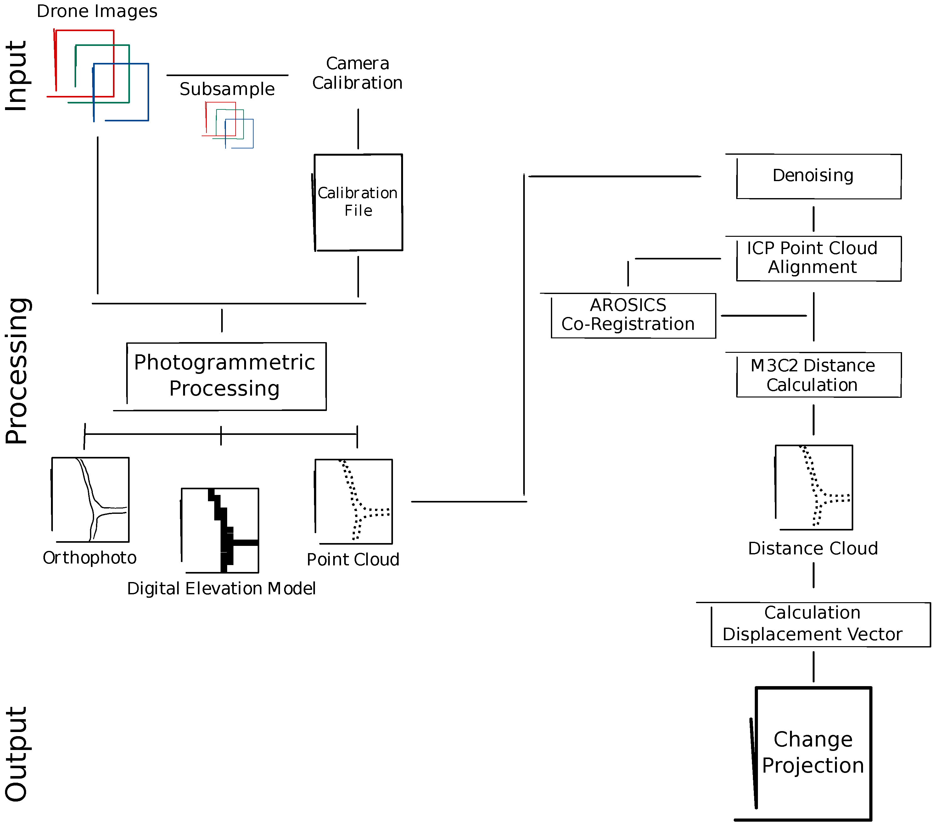
2.3. Photogrammetric Processing
2.3.1. Calibration
2.3.2. Photogrammetric Processing
2.4. Point Cloud Processing
2.4.1. Denoising
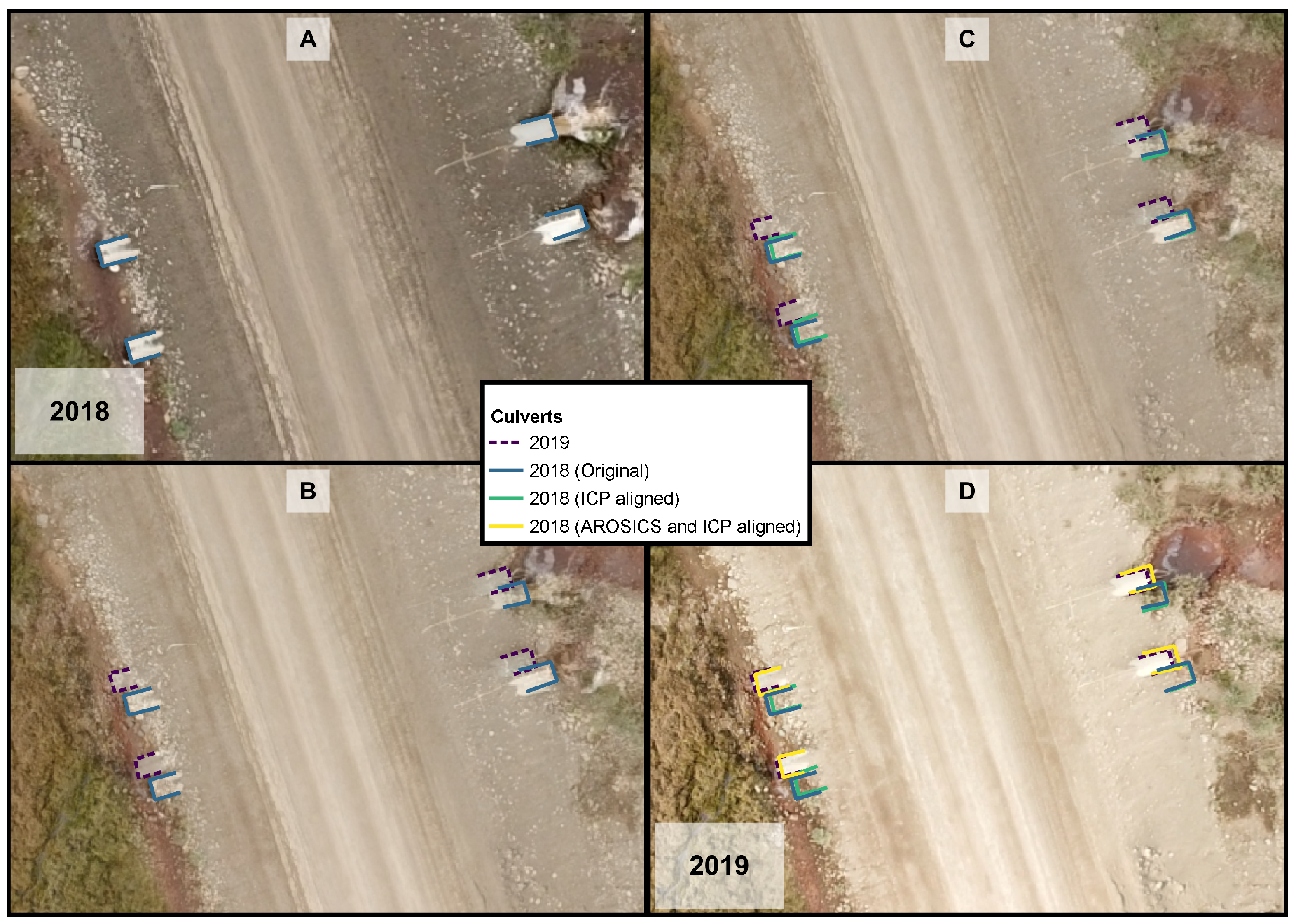
2.4.2. Registration
- The iteration process was set to stop when a root mean square error (RMS) difference of m was reached. This small threshold value comes with a high computation time but a very accurate alignment [35].
- In 2019, the UAV captured slightly more images. We therefore set the theoretical overlap of the clouds for user scenario 2 at 85% (90% of the area extent in 2019 were covered in 2018, an additional 5% were set as a an uncertainty buffer). Due to the exclusion of the erosion feature and the vehicles the overlap was set at 80% for user scenario 1.
- CloudCompare aims at optimizing the computation speed. Therefore, it implemented a random sampling limit that describes a maximum number of points which are randomly sub-sampled from the cloud for each iteration [35]. The limit was set to 70,000 points with the farthest point removal enabled. The latter led to an elimination of points that are too far away from the reference cloud.
2.5. Repetition with AROSICS
2.6. Ground Truthing
2.7. Change Detection
2.8. Change Projection
3. Results
3.1. Accuracy Assessment
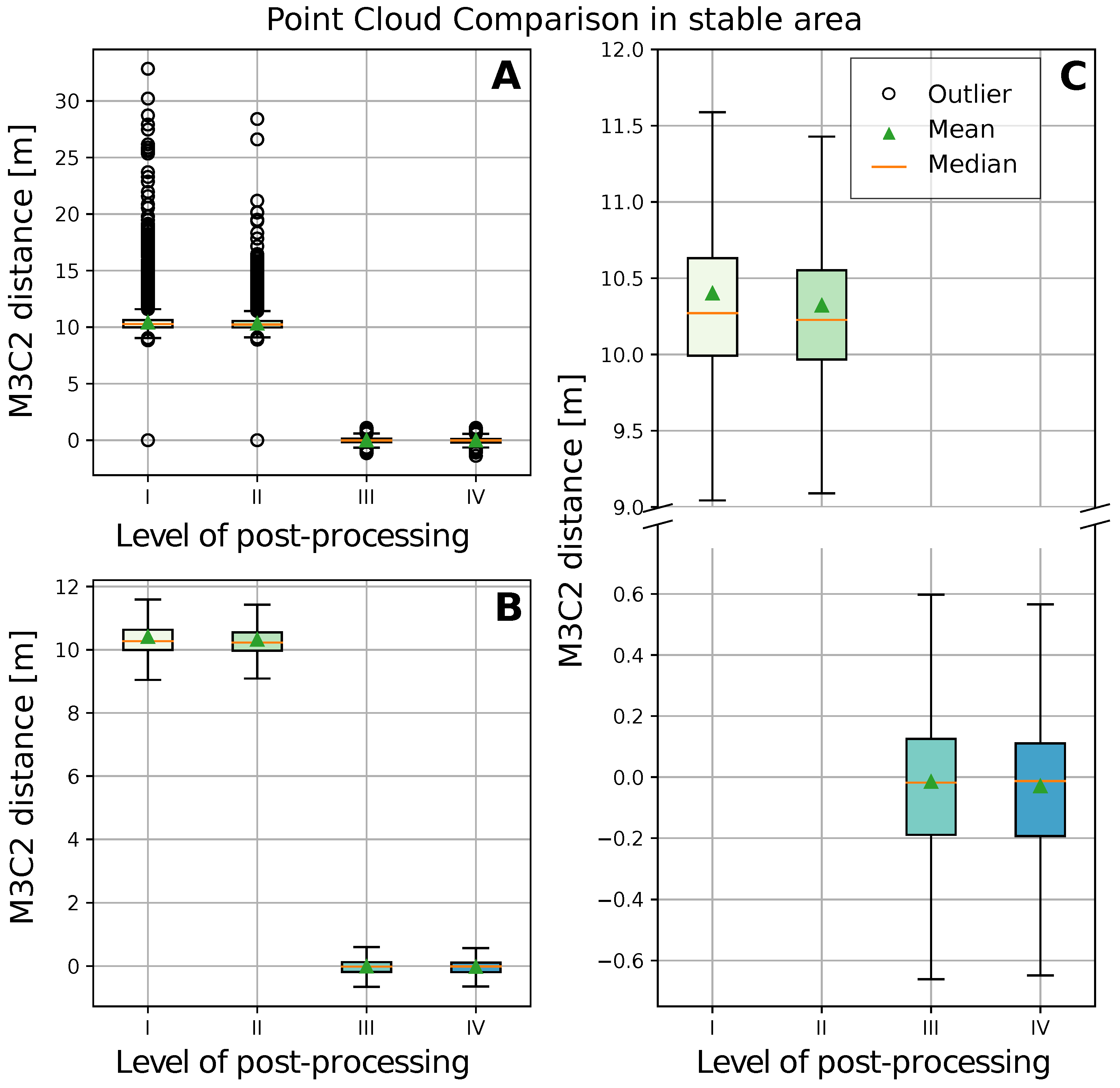
3.1.1. Whole Study Area
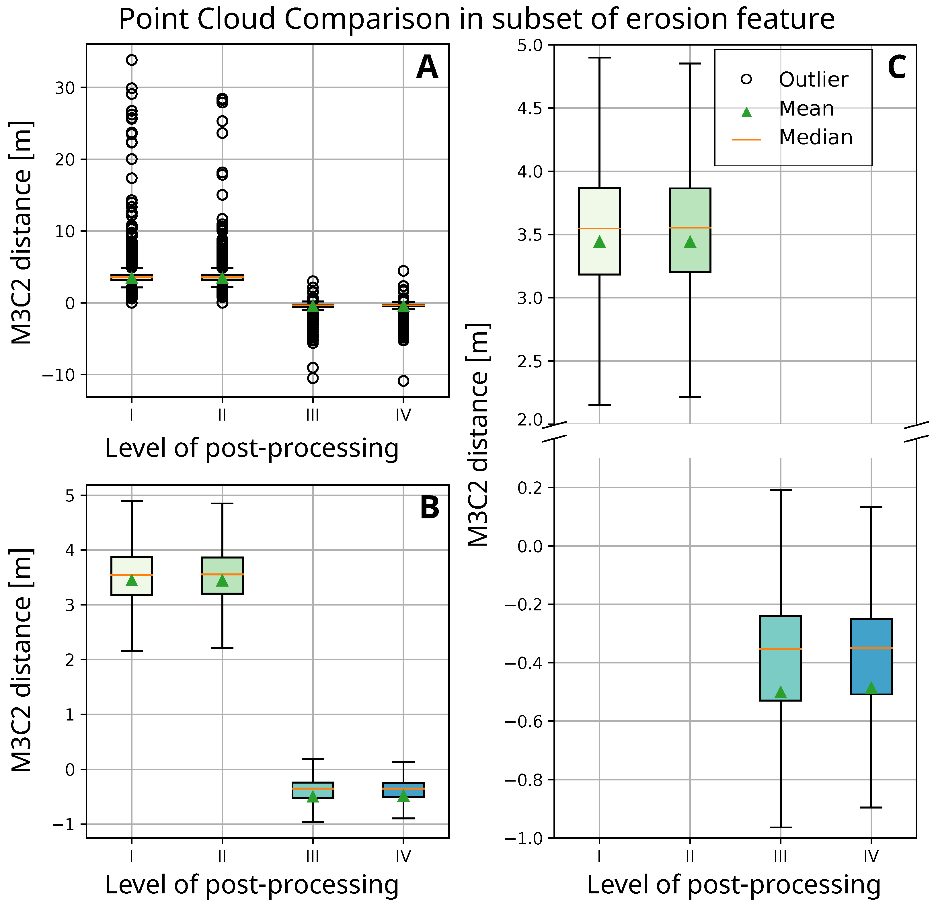
3.1.2. Subsets of Study Area
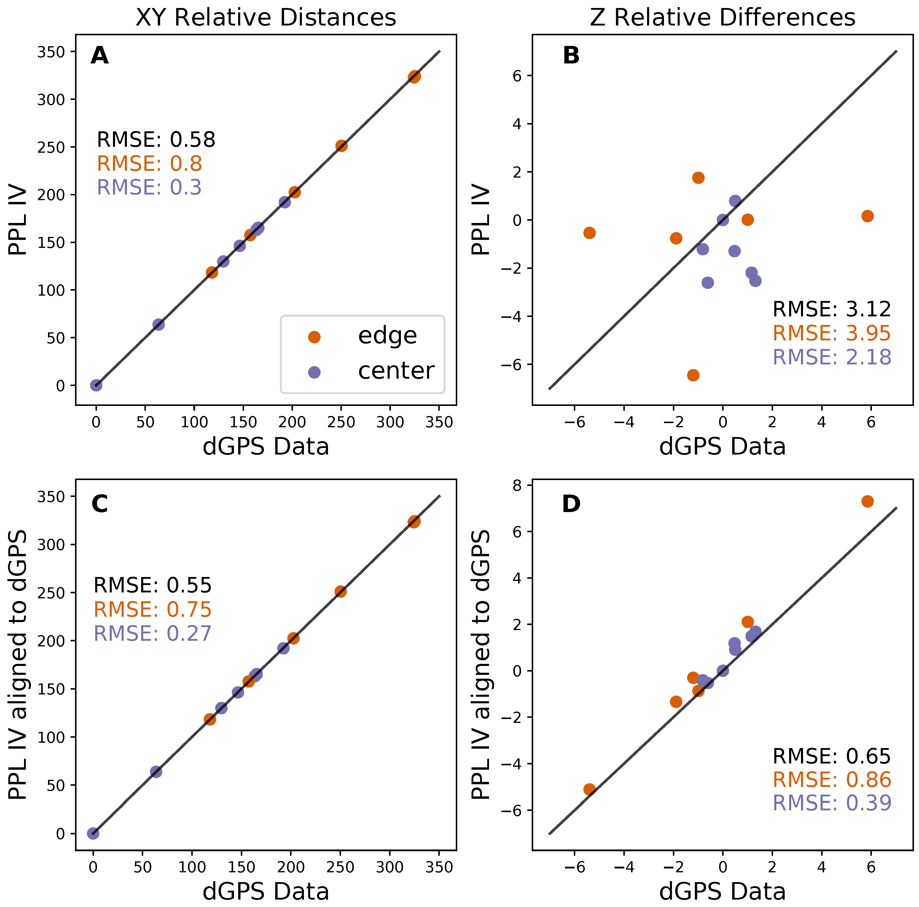
3.1.3. Ground Truthing
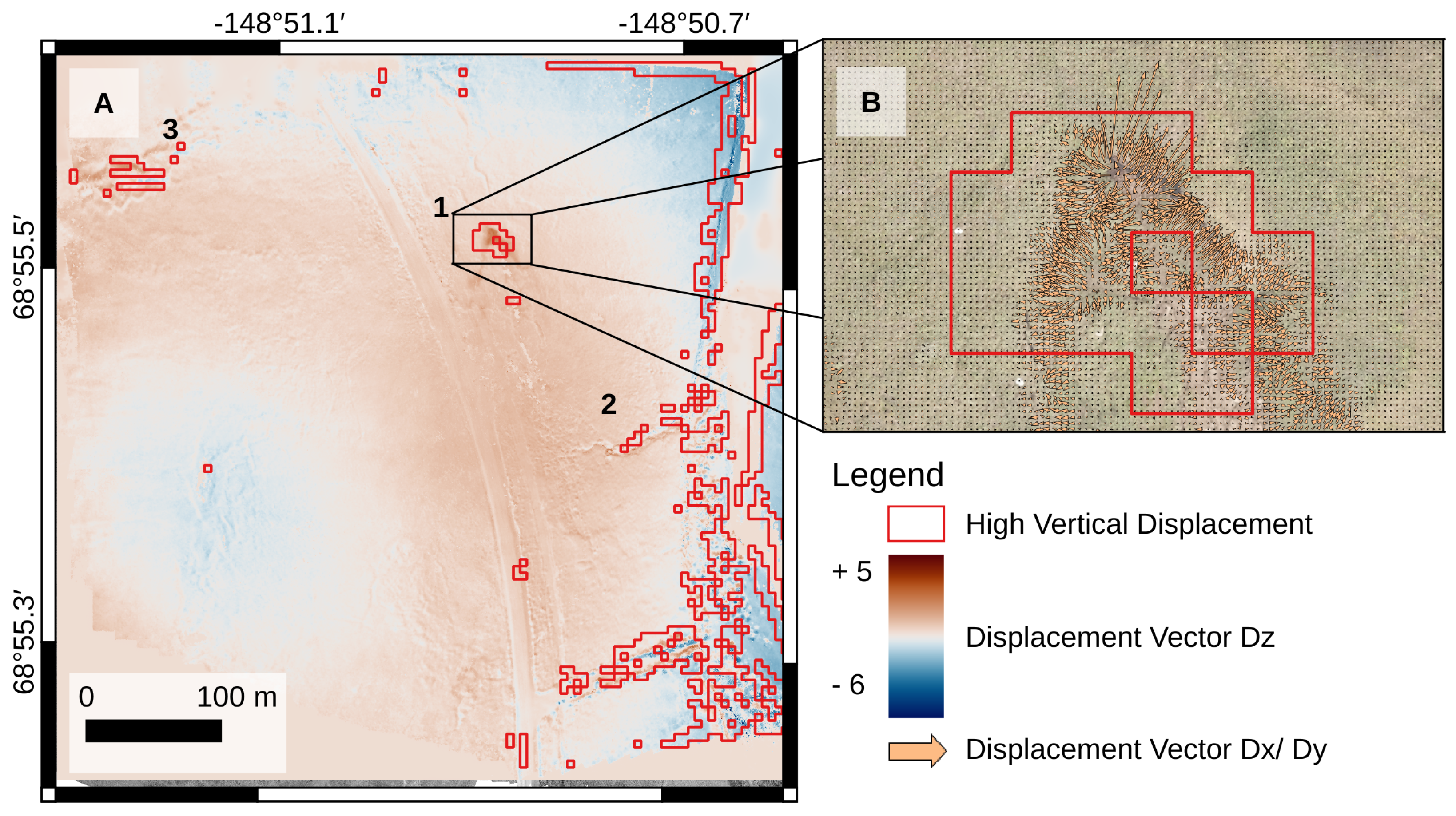
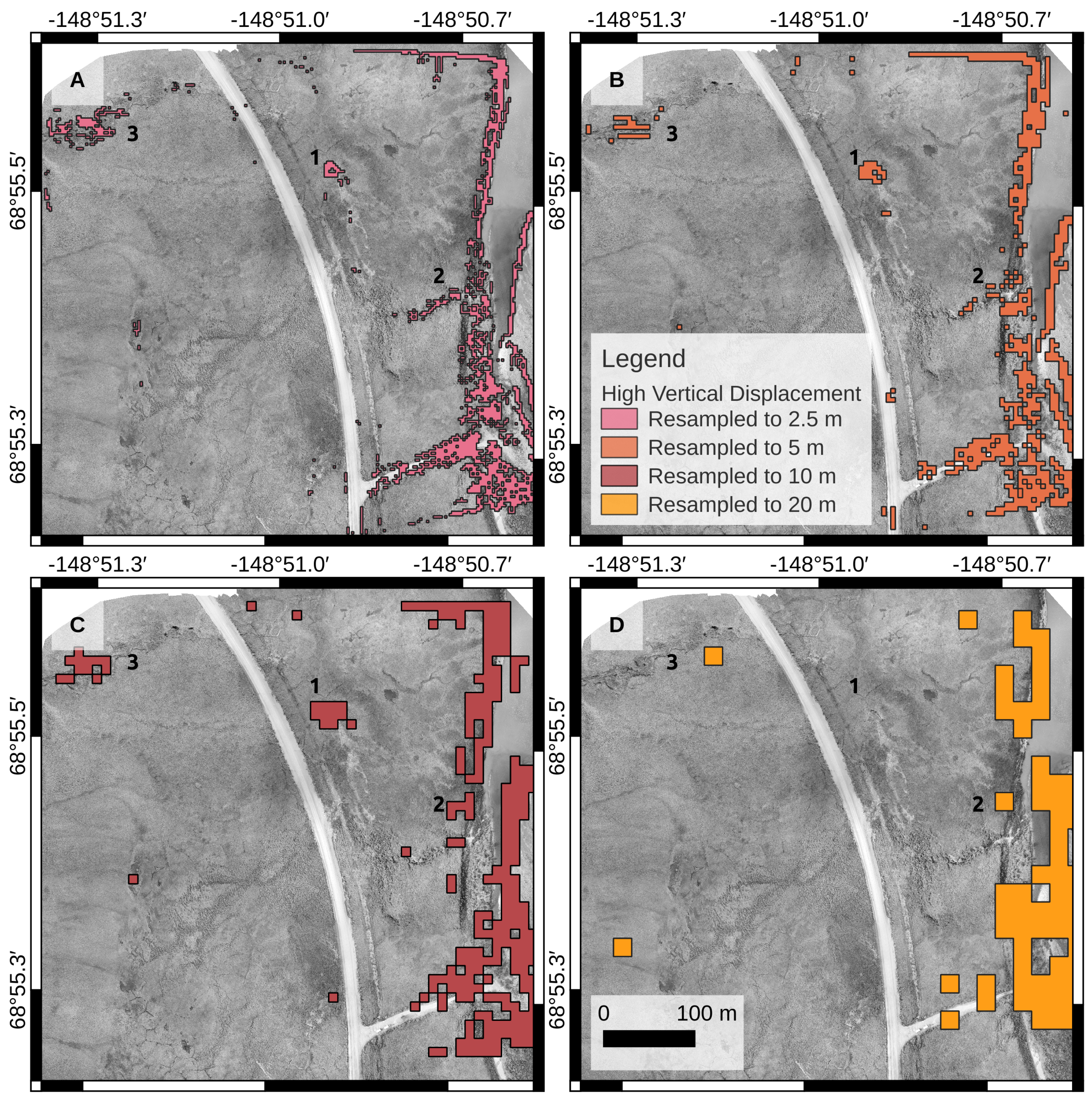
3.2. Change Detection and Projection
4. Discussion
5. Conclusions
Author Contributions
Funding
Data Availability Statement
Acknowledgments
Conflicts of Interest
Abbreviations
| AROSICS | Automated and Robust Open-Source Image Co-Registration Software |
| ICP | Iterative Closest Point |
| IDW | Inverse Distance Weighting |
| IQR | Interquartile Range |
| kNN | k-Nearest Neighbour |
| M3C2 | Multiscale Model to Model Cloud Comparison |
| ODM | OpenDroneMap |
| POI | Point of Interest |
| SfM | Structure from Motion |
| UAV | Unoccupied Aerial Vehicle |
Appendix A

| Processing Step | Explanation |
|---|---|
| Load Dataset: | ODM reads metadata from the EXIF (Exchangeable Image File Format) tags of all images, containing information on geolocation (GPS) |
| Structure from Motion: | The photogrammetry technique computes the camera’s position and angle (camera pose) for every image by looking for unique features that are visible in both (or more) images [25]. This allows the creation of a sparse point cloud [25]. OpenDroneMap uses the Python library OpenSfM [51,52]. |
| Multi-View Stereo (MVS): | Complementing the SfM technique, MVS uses the derived camera information and sparse point cloud to produce a highly detailed (dense) point cloud [25]. |
| Meshing: | In this step, the 3D points of the cloud are connected to form triangles forming a polygonal mesh. |
| Texturing: | The mesh, the camera poses and the images build the basis for the texturing. Every polygon of the mesh is assigned the best fitting image from which the colour is derived [25]. MvsTexturing is the software used by OpenDroneMap [53]. |
| Georeferencing: | This step contains the transformation of local coordinates to the actual geographic coordinates. The information on the world coordinate system is extracted from the images’ GPS tags. |
| Digital Elevation Model Processing: | ODM uses the georeferenced point cloud and applies an inverse distance weighting interpolation (IDW) method to extract a surface model [25]. Missing values (gaps) in the model are filled within IDW interpolation and noise is filtered using a median filter [25]. |
| Orthophoto Processing: | In the last step the textured 3D mesh is loaded into an orthographic scene and is virtually captured and saved from above as an image. The result is a georeferenced orthophoto, cropped to its geolocation boundaries [25]. |


References
- Arias, P.A.; Bellouin, N.; Coppola, E.; Jones, R.G.; Krinner, G.; Marotzke, J.; Naik, V.; Palmer, M.D.; Plattner, G.K.; Rogelj, J.; et al. Technical Summary. In Climate Change 2021: The Physical Science Basis; Cambridge University Press: Cambridge, UK; New York, NY, USA, 2021; pp. 33–144. [Google Scholar] [CrossRef]
- Rowland, J.C.; Jones, C.E.; Altmann, G.; Bryan, R.; Crosby, B.T.; Hinzman, L.D.; Kane, D.L.; Lawrence, D.M.; Mancino, A.; Marsh, P.; et al. Arctic Landscapes in Transition: Responses to Thawing Permafrost. Eos Trans. Am. Geophys. Union 2010, 91, 229–230. [Google Scholar] [CrossRef]
- Nitze, I.; Grosse, G.; Jones, B.M.; Romanovsky, V.E.; Boike, J. Remote sensing quantifies widespread abundance of permafrost region disturbances across the Arctic and Subarctic. Nat. Commun. 2018, 9, 5423. [Google Scholar] [CrossRef] [PubMed]
- Runge, A.; Nitze, I.; Grosse, G. Remote sensing annual dynamics of rapid permafrost thaw disturbances with LandTrendr. Remote Sens. Environ. 2022, 268, 112752. [Google Scholar] [CrossRef]
- Kaiser, S.; Grosse, G.; Boike, J.; Langer, M. Monitoring the Transformation of Arctic Landscapes: Automated Shoreline Change Detection of Lakes Using Very High Resolution Imagery. Remote Sens. 2021, 13, 2802. [Google Scholar] [CrossRef]
- Nelson, F.E.; Anisimov, O.A.; Shiklomanov, N.I. Subsidence risk from thawing permafrost. Nature 2001, 410, 889–890. [Google Scholar] [CrossRef]
- Liljedahl, A.K.; Boike, J.; Daanen, R.P.; Fedorov, A.N.; Frost, G.V.; Grosse, G.; Hinzman, L.D.; Iijma, Y.; Jorgenson, J.C.; Matveyeva, N.; et al. Pan-Arctic ice-wedge degradation in warming permafrost and its influence on tundra hydrology. Nat. Geosci. 2016, 9, 312–318. [Google Scholar] [CrossRef]
- Hjort, J.; Streletskiy, D.; Doré, G.; Wu, Q.; Bjella, K.; Luoto, M. Impacts of permafrost degradation on infrastructure. Nat. Rev. Earth Environ. 2022, 3, 24–38. [Google Scholar] [CrossRef]
- Hjort, J.; Karjalainen, O.; Aalto, J.; Westermann, S.; Romanovsky, V.E.; Nelson, F.E.; Etzelmüller, B.; Luoto, M. Degrading permafrost puts Arctic infrastructure at risk by mid-century. Nat. Commun. 2018, 9, 5147. [Google Scholar] [CrossRef]
- Liew, M.; Xiao, M.; Farquharson, L.; Nicolsky, D.; Jensen, A.; Romanovsky, V.; Peirce, J.; Alessa, L.; McComb, C.; Zhang, X.; et al. Understanding Effects of Permafrost Degradation and Coastal Erosion on Civil Infrastructure in Arctic Coastal Villages: A Community Survey and Knowledge Co-Production. J. Mar. Sci. Eng. 2022, 10, 422. [Google Scholar] [CrossRef]
- Armstrong, L.; Lacelle, D.; Fraser, R.H.; Kokelj, S.; Knudby, A. Thaw slump activity measured using stationary cameras in time-lapse and Structure-from-Motion photogrammetry. Arct. Sci. 2018, 4, 827–845. [Google Scholar] [CrossRef]
- Clark, A.; Moorman, B.; Whalen, D.; Fraser, P. Arctic coastal erosion: Uav-sfm data collection strategies for planimetric and volumetric measurements. Arct. Sci. 2021, 7, 605–633. [Google Scholar] [CrossRef]
- Turner, K.W.; Pearce, M.D.; Hughes, D.D. Detailed characterization and monitoring of a retrogressive thaw slump from remotely piloted aircraft systems and identifying associated influence on carbon and nitrogen export. Remote Sens. 2021, 13, 171. [Google Scholar] [CrossRef]
- Van der Sluijs, J.; Kokelj, S.V.; Fraser, R.H.; Tunnicliffe, J.; Lacelle, D. Permafrost Terrain Dynamics and Infrastructure Impacts Revealed by UAV Photogrammetry and Thermal Imaging. Remote Sens. 2018, 10, 1734. [Google Scholar] [CrossRef]
- CAVM Team. Circumpolar Arctic Vegetation Map. (1:7,500,000 Scale), Conservation of Arctic Flora and Fauna (CAFF) Map No. 1; US Fish and Wildlife Service: Anchorage, AK, USA, 2003; Available online: https://www.geobotany.uaf.edu/cavm/ (accessed on 28 November 2022).
- Gallant, A.L.; Binnian, E.F.; Omernik, J.M.; Shasby, M.B. Ecoregions of Alaska. Technical Report. 1995. Available online: https://ngmdb.usgs.gov/Prodesc/proddesc_4931.htm (accessed on 28 November 2022).
- Raynolds, M.K.; Walker, D.A.; Ambrosius, K.J.; Brown, J.; Everett, K.R.; Kanevskiy, M.; Kofinas, G.P.; Romanovsky, V.E.; Shur, Y.; Webber, P.J. Cumulative geoecological effects of 62 years of infrastructure and climate change in ice-rich permafrost landscapes, Prudhoe Bay Oilfield, Alaska. Glob. Chang. Biol. 2014, 20, 1211–1224. [Google Scholar] [CrossRef]
- Bhuiyan, M.A.E.; Witharana, C.; Liljedahl, A.K. Use of Very High Spatial Resolution Commercial Satellite Imagery and Deep Learning to Automatically Map Ice-Wedge Polygons across Tundra Vegetation Types. J. Imaging 2020, 6, 137. [Google Scholar] [CrossRef]
- Porter, C.; Morin, P.; Howat, I.; Noh, M.J.; Bates, B.; Peterman, K.; Keesey, S.; Schlenk, M.; Gardiner, J.; Tomko, K.; et al. ArcticDEM, version 3. 2018. Available online: https://dataverse.harvard.edu/dataset.xhtml?persistentId=doi:10.7910/DVN/OHHUKH (accessed on 28 November 2022).
- Alaska Oil and Gas Association. The Role of the Oil and Gas Industry in Alaska’s Economy. Technical Report January. 2020. Available online: https://www.aoga.org/wp-content/uploads/2021/01/Reports-2020.1.23-Economic-Impact-Report-McDowell-Group-CORRECTED-2020.12.3.pdf (accessed on 28 November 2022).
- DJI. Mavic Pro. User Manual V2.0, 2017.12. 2017. Available online: https://dl.djicdn.com/downloads/mavic/Mavic_Pro_User_Manual_v2.0_en.pdf (accessed on 3 January 2022).
- Drone Harmony AG. Data Capture Platform for Drones & UAVs. 2022. Available online: https://droneharmony.com/ (accessed on 3 January 2022).
- Drone Harmony AG. Drone Harmony. The Plan Catalog. 2021. Available online: https://droneharmony.com/docs/the-plan-catalog/ (accessed on 3 January 2022).
- Rosnell, T.; Honkavaara, E. Point cloud generation from aerial image data acquired by a quadrocopter type micro unmanned aerial vehicle and a digital still camera. Sensors 2012, 12, 453–480. [Google Scholar] [CrossRef]
- Toffanin, P. OpenDroneMap: The Missing Guide, 1st ed.; UAV4GEO: St. Petersburg, FL, USA, 2019. [Google Scholar]
- James, M.R.; Robson, S. Mitigating systematic error in topographic models derived from UAV and ground-based image networks. Earth Surf. Process. Landforms 2014, 39, 1413–1420. [Google Scholar] [CrossRef]
- Nesbit, P.R.; Hugenholtz, C.H. Enhancing UAV-SfM 3D model accuracy in high-relief landscapes by incorporating oblique images. Remote Sens. 2019, 11, 239. [Google Scholar] [CrossRef]
- UAV4GEO. Drone & UAV Mapping Software|WebODM. Available online: https://webodm.net/ (accessed on 3 January 2022).
- OpenDroneMap Authors. ODM—A Command Line Toolkit to Generate Maps, Point Clouds, 3D Models and DEMs from Drone, Balloon or Kite Images. OpenDroneMap/ODM GitHub Page. Available online: https://github.com/OpenDroneMap/ODM (accessed on 28 November 2022).
- Pingel, T.J.; Clarke, K.C.; McBride, W.A. An improved simple morphological filter for the terrain classification of airborne LIDAR data. ISPRS J. Photogramm. Remote Sens. 2013, 77, 21–30. [Google Scholar] [CrossRef]
- OpenDroneMap Authors. Tutorials—Creating Digital Elevation Models. 2020. Available online: https://docs.opendronemap.org/tutorials/ (accessed on 28 November 2022).
- Girardeau-Montaut, D. Cloud Compare—Open Source Project. Available online: https://www.cloudcompare.org/ (accessed on 3 January 2022).
- Girardeau-Montaut, D. CloudCompareWiki. 2016. Available online: https://www.cloudcompare.org/doc/wiki/index.php?title=Main_Page (accessed on 3 January 2022).
- Girardeau-Montaut, D. Noise Filter—CloudCompareWiki. 2015. Available online: https://www.cloudcompare.org/doc/wiki/index.php?title=Noise_filter (accessed on 3 January 2022).
- Girardeau-Montaut, D. ICP—CloudCompareWiki. 2015. Available online: https://www.cloudcompare.org/doc/wiki/index.php?title=ICP (accessed on 3 January 2022).
- Scheffler, D.; Hollstein, A.; Diedrich, H.; Segl, K.; Hostert, P. AROSICS: An Automated and Robust Open-Source Image Co-Registration Software for Multi-Sensor Satellite Data. Remote Sens. 2017, 9, 676. [Google Scholar] [CrossRef]
- James, M.R.; Antoniazza, G.; Robson, S.; Lane, S.N. Mitigating systematic error in topographic models for geomorphic change detection: Accuracy, precision and considerations beyond off-nadir imagery. Earth Surf. Process. Landforms 2020, 45, 2251–2271. [Google Scholar] [CrossRef]
- Lague, D.; Brodu, N.; Leroux, J. Accurate 3D comparison of complex topography with terrestrial laser scanner: Application to the Rangitikei canyon (N-Z). ISPRS J. Photogramm. Remote Sens. 2013, 82, 10–26. [Google Scholar] [CrossRef]
- Barnhart, T.B.; Crosby, B.T. Comparing Two Methods of Surface Change Detection on an Evolving Thermokarst Using High-Temporal-Frequency Terrestrial Laser Scanning, Selawik River, Alaska. Remote Sens. 2013, 5, 2813–2837. [Google Scholar] [CrossRef]
- Bash, E.A.; Moorman, B.J.; Gunther, A. Detecting Short-Term Surface Melt on an Arctic Glacier Using UAV Surveys. Remote Sens. 2018, 10, 1547. [Google Scholar] [CrossRef]
- Stumpf, A.; Malet, J.P.; Allemand, P.; Pierrot-Deseilligny, M.; Skupinski, G. Ground-based multi-view photogrammetry for the monitoring of landslide deformation and erosion. Geomorphology 2015, 231, 130–145. [Google Scholar] [CrossRef]
- Pedregosa, F.; Varoquaux, G.; Gramfort, A.; Michel, V.; Thirion, B.; Grisel, O.; Blondel, M.; Prettenhofer, P.; Weiss, R.; Dubourg, V.; et al. Scikit-learn: Machine Learning in Python. J. Mach. Learn. Res. 2011, 12, 2825–2830. Available online: https://jmlr.org/papers/volume12/pedregosa11a/pedregosa11a.pdf (accessed on 28 November 2022).
- Kalacska, M.; Lucanus, O.; Arroyo-Mora, J.P.; Laliberté, É.; Elmer, K.; Leblanc, G.; Groves, A. Accuracy of 3D Landscape Reconstruction without Ground Control Points Using Different UAS Platforms. Drones 2020, 4, 13. [Google Scholar] [CrossRef]
- Farquharson, L.M.; Romanovsky, V.E.; Cable, W.L.; Walker, D.A.; Kokelj, S.V.; Nicolsky, D. Climate Change Drives Widespread and Rapid Thermokarst Development in Very Cold Permafrost in the Canadian High Arctic. Geophys. Res. Lett. 2019, 46, 6681–6689. [Google Scholar] [CrossRef]
- Zwieback, S.; Meyer, F.J. Top-of-permafrost ground ice indicated by remotely sensed late-season subsidence. Cryosphere 2021, 15, 2041–2055. [Google Scholar] [CrossRef]
- Shiklomanov, N.I.; Streletskiy, D.A.; Little, J.D.; Nelson, F.E. Isotropic thaw subsidence in undisturbed permafrost landscapes. Geophys. Res. Lett. 2013, 40, 6356–6361. [Google Scholar] [CrossRef]
- Westermann, S.; Langer, M.; Boike, J.; Heikenfeld, M.; Peter, M.; Etzelmüller, B.; Krinner, G. Simulating the thermal regime and thaw processes of ice-rich permafrost ground with the land-surface model CryoGrid 3. Geosci. Model Dev. 2016, 9, 523–546. [Google Scholar] [CrossRef]
- Nitzbon, J.; Westermann, S.; Langer, M.; Martin, L.C.; Strauss, J.; Laboor, S.; Boike, J. Fast response of cold ice-rich permafrost in northeast Siberia to a warming climate. Nat. Commun. 2020, 11, 2201. [Google Scholar] [CrossRef] [PubMed]
- Papakonstantinou, A.; Batsaris, M.; Spondylidis, S.; Topouzelis, K. A Citizen Science Unmanned Aerial System Data Acquisition Protocol and Deep Learning Techniques for the Automatic Detection and Mapping of Marine Litter Concentrations in the Coastal Zone. Drones 2021, 5, 6. [Google Scholar] [CrossRef]
- Zahs, V.; Winiwarter, L.; Anders, K.; Williams, J.G.; Rutzinger, M.; Höfle, B. Correspondence-driven plane-based M3C2 for lower uncertainty in 3D topographic change quantification. ISPRS J. Photogramm. Remote Sens. 2022, 183, 541–559. [Google Scholar] [CrossRef]
- GitHub–Mapillary/OpenSfM: Open Source Structure-from-Motion Pipeline. 2020. Available online: https://github.com/mapillary/OpenSfM (accessed on 3 January 2022).
- Groos, A.R.; Bertschinger, T.J.; Kummer, C.M.; Erlwein, S.; Munz, L.; Philipp, A. The Potential of Low-Cost UAVs and Open-Source Photogrammetry Software for High-Resolution Monitoring of Alpine Glaciers: A Case Study from the Kanderfirn (Swiss Alps). Geosciences 2019, 9, 356. [Google Scholar] [CrossRef]
- Moehrle, N. GitHub-Nmoehrle/mvs-Texturing: Algorithm to Texture 3D Reconstructions from Multi-View Stereo Images. 2020. Available online: https://github.com/nmoehrle/mvs-texturing (accessed on 3 January 2022).


| Acquisition Date | Number of Images | GSD [cm] | Orthophoto Mosaic [cm] | DSM [cm] |
|---|---|---|---|---|
| 7 August 2018 | 445 | 4 | 17 | |
| 18 June 2019 | 522 | 4 | 18 |
| Parameter | Explanation | Value |
|---|---|---|
| –dsm | Generates a Digital Surface Model (including vegetation). | True |
| –dtm | Generates a Digital Terrain Model. For distinguishing between ground and non-ground objects ODM uses a simple morphological filter (SMRF) [30]. We adjust the SMRF parameters in order to properly present the lowland tundra environment, see smrf-threshold, -window, -scalar and -slope [31]. | True |
| –pc-classify | The activation of pc-classify is mandatory to generate both, a Digital Terrain Model and Digital Surface Model. It enables parameter tweaking of SMRF to distinguish between ground- and non-ground objects [25]. | True |
| –smrf-threshold | Set to the minimum height (in m) of non-ground objects, which in our study area are mostly shrubs (Default: ). | |
| –smrf-window | Set to the size of the largest non-ground object (in m). Kept at the recommended minimum value of (Default: ). | 10 |
| –smrf-scalar | Describes the dependence between the threshold and slope. It is recommended to increase this value slightly when minimizing the default smrf-threshold value (Default: ). | |
| –smrf-slope | Describes terrain slope of study area. Derived from the ratio between elevation change and horizontal distance change. The value corresponds to a change of 50 cm over a 10 m distance (Default: ). Differential GPS data of the study area show a maximum elevation change of 20 cm over a 10 m distance. To also account for the Dalton Highway we chose a value of . | |
| –depthmap-resolution | Refers to an image containing information on the distance between camera and object: dark parts of the image are closer, bright parts farther away from the camera. Images are used to generate the point cloud. With an increasing value, the level of detail increases but also the occurrence of noise. We chose a value in between the default (640) and maximum (1000 [28]) to produce a high density point cloud while at the same time trying to mitigate a high amount of noise. | 800 |
| –use-opensfm-dense | Enables the use of the Python library OpenSfM for the Multi-View processing step (opposed to the default using the software suits Multi-View Environment). The activation of use-opensfm-dense is mandatory when defining the depthmap-resolution [25]. | True |
| 2018 | 2019 | |||
|---|---|---|---|---|
| Point Cloud | Number of Points | (%) | Number of Points | (%) |
| Raw | 70,574,548 | 100 | 84,731,227 | 100 |
| Denoised | ||||
| — ball radius | 60,746,799 | 86 | 68,806,542 | 81 |
| — kNN4 | 49,260,479 | 70 | 61,522,497 | 73 |
| Reference Cloud 2018 | Reference Cloud 2019 | |||
|---|---|---|---|---|
| Post-Processing Level III | kNN4 | Ball Radius | kNN4 | Ball Radius |
| unsupervised alignment | 1.07 | 1.12 | 1.05 | 1.07 |
| supervised alignment | 1.00 | 1.05 | 0.98 | 1.00 |
| Post-Processing Level IV | ||||
| unsupervised alignment | – | – | 1.05 | – |
| supervised alignment | – | – | 0.99 | – |
Publisher’s Note: MDPI stays neutral with regard to jurisdictional claims in published maps and institutional affiliations. |
© 2022 by the authors. Licensee MDPI, Basel, Switzerland. This article is an open access article distributed under the terms and conditions of the Creative Commons Attribution (CC BY) license (https://creativecommons.org/licenses/by/4.0/).
Share and Cite
Kaiser, S.; Boike, J.; Grosse, G.; Langer, M. The Potential of UAV Imagery for the Detection of Rapid Permafrost Degradation: Assessing the Impacts on Critical Arctic Infrastructure. Remote Sens. 2022, 14, 6107. https://doi.org/10.3390/rs14236107
Kaiser S, Boike J, Grosse G, Langer M. The Potential of UAV Imagery for the Detection of Rapid Permafrost Degradation: Assessing the Impacts on Critical Arctic Infrastructure. Remote Sensing. 2022; 14(23):6107. https://doi.org/10.3390/rs14236107
Chicago/Turabian StyleKaiser, Soraya, Julia Boike, Guido Grosse, and Moritz Langer. 2022. "The Potential of UAV Imagery for the Detection of Rapid Permafrost Degradation: Assessing the Impacts on Critical Arctic Infrastructure" Remote Sensing 14, no. 23: 6107. https://doi.org/10.3390/rs14236107
APA StyleKaiser, S., Boike, J., Grosse, G., & Langer, M. (2022). The Potential of UAV Imagery for the Detection of Rapid Permafrost Degradation: Assessing the Impacts on Critical Arctic Infrastructure. Remote Sensing, 14(23), 6107. https://doi.org/10.3390/rs14236107