
Modelling and Mapping of Soil Erosion Susceptibility of Murree, Sub-Himalayas Using GIS and RS-Based Models

 ,
,  ,
,  ,
, 

Abstract
1. Introduction
2. Study Area
3. Materials and Methods
3.1. Datasets
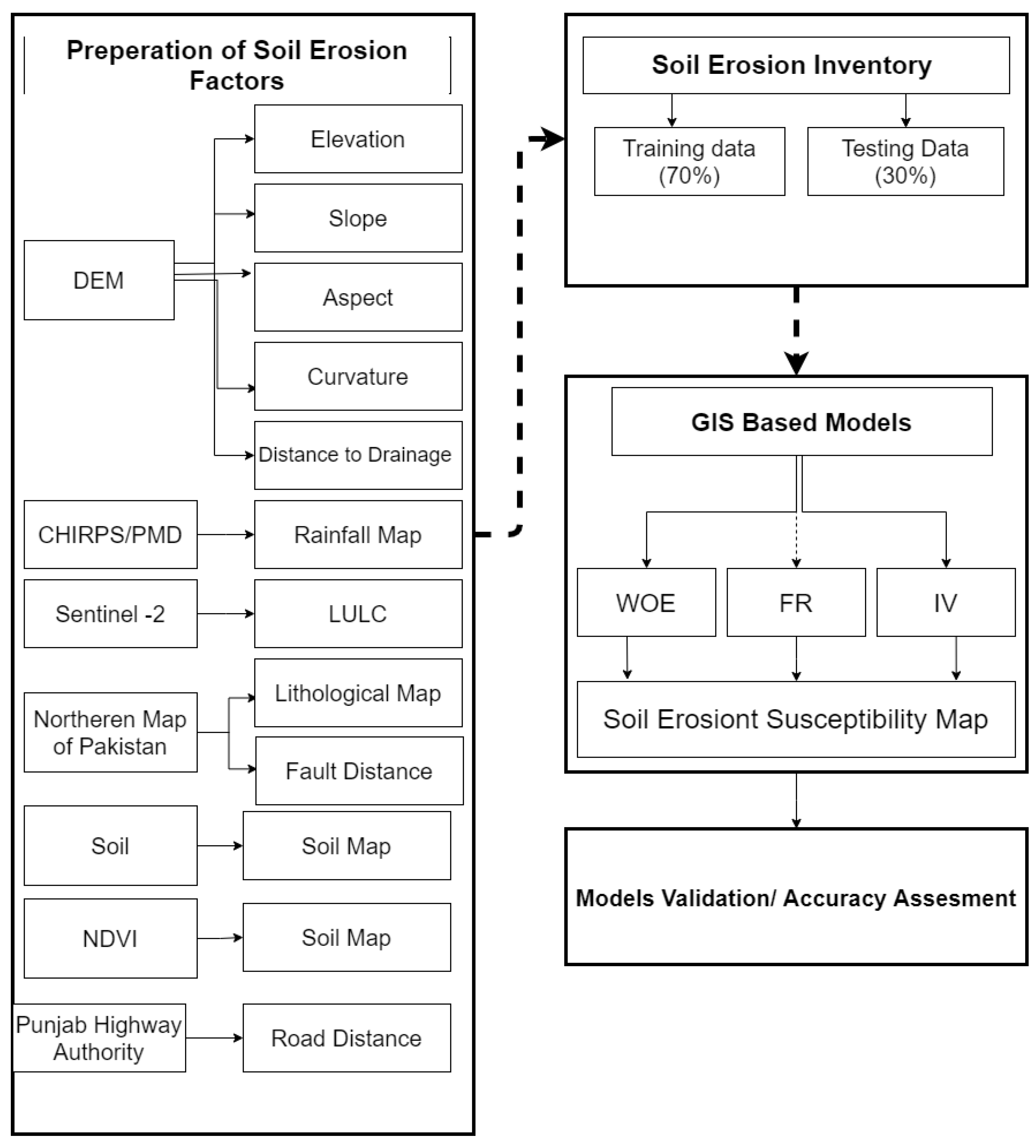
3.2. Methods
3.2.1. Soil Erosion Inventory Map
3.2.2. Production of the Thematic Data Layers
- (i)
- Elevation: The elevation of the land influences the type of plants and the pattern of rainfall [43]. SRTM data with a spatial resolution of 30 m was used to obtain the elevation of the research area. Using the natural break technique, as shown in Figure 3a, the elevation was separated into different classes.
- (ii)
- Slope: Slope is an important element in soil erosion because the angle of the slope impacts water penetration and velocity; thus, gentle slopes and flat areas have less soil erosion than steep gradients and slope length [44]. As illustrated in Figure 3b, the slop of the research region was estimated using an SRTM DEM with a resolution of 30 m and reclassified into five classes using ArcGIS 10.8.
- (iii)
- (iv)
- (v)
- Drainage: Stream channels have a significant impact on the shear strength of rocks and the erosion of sediment [28]. The stream network was extracted from the SRTM DEM and a five-class buffer was applied to the stream network to understand the relationship between soil erosion and drainage network, as illustrated in Figure 4a.
- (vi)
- Rainfall: Precipitation is a crucial causal feature of soil erosion because it causes particle dissociation and accelerates soil erosion [46]. The erosivity of precipitation is a primary driving element for sheet and rill erosion. The present research area’s rainfall map was generated from CHIRPS data using a machine learning approach. As illustrated in Figure 4b, the final rainfall map was categorized into five groups using the ArcGIS 10.8 platform.
- (vii)
- UIC: LULC change has a significant impact on soil erosion, independent of other predisposing factors such as climate, soil properties, and topography [47]. The research area’s LULC map was generated in GEE using a machine learning approach employing high resolution data. As illustrated in Figure 4c, the LULC map was exported into ArcGIS and reclassified into five groups to examine the various classes of LULC with soil erosion.
- (viii)
- Geology: The composition of different types of rocks, such as volcanic, sedimentary, and metamorphic rocks, as well as their geological formations, have varying effects on soil erosion [48]. Figure 4d depicts the lithological map of the research region, which was digitized from the Northern Geological Map of Pakistan.
- (ix)
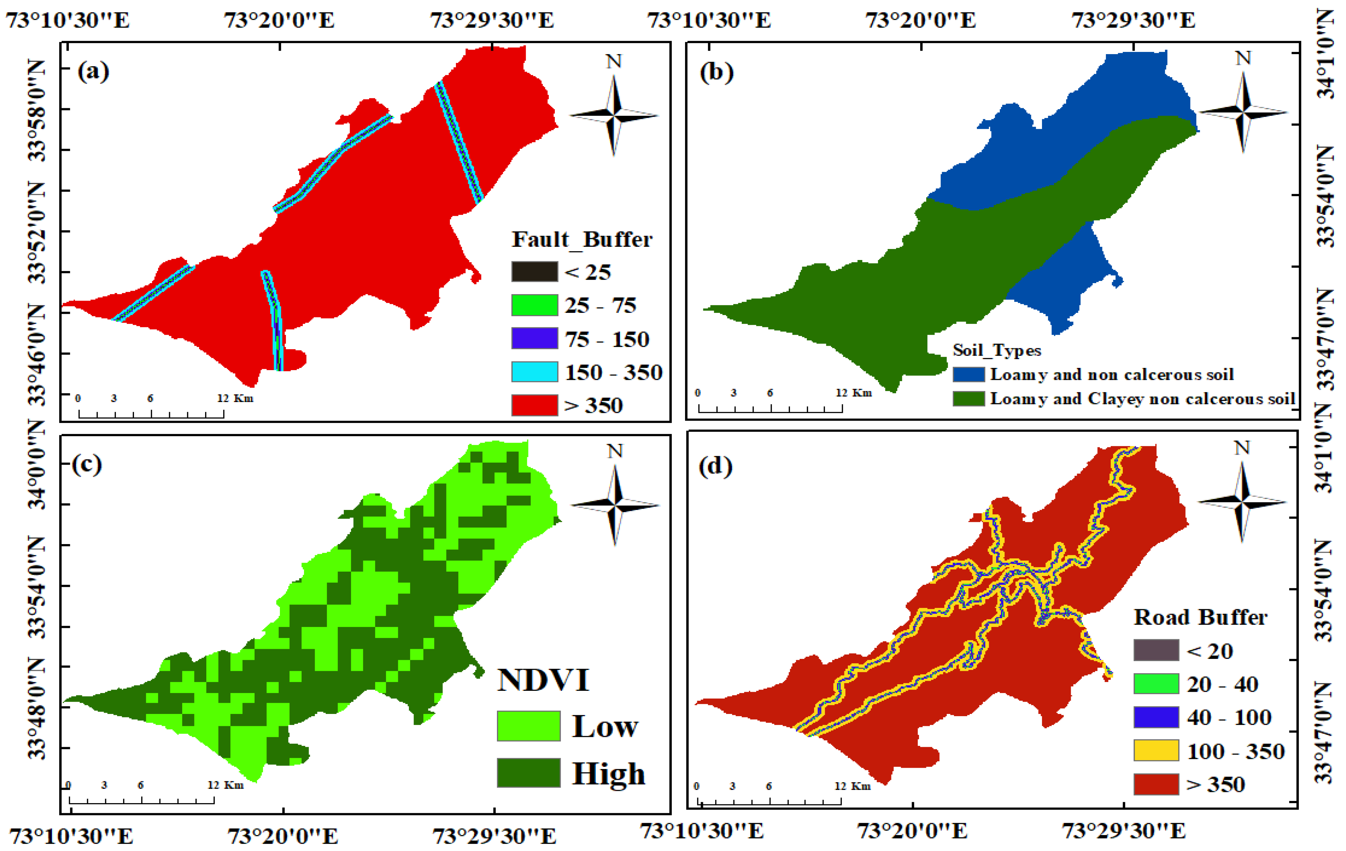
- Fault: A fault is a lithological feature that has deformed the rocks in the studied region. Figure 5a shows a fault map that was digitized from a geological map of North Pakistan. Following digitization, five buffers were used to estimate the association fault with soil erosion.
- (x)
- Soil: The texture of the soil surface is an important predisposing factor of soil erosion since the texture and structure of the soil impact soil resistance to erosion because structural stability and plant cover reduce soil erosion [43]. Figure 5b depicts the soil map of the study region obtained from a soil survey in Pakistan.
- (xi)
- NDVI: Vegetation cover reduces soil erosion and may affect the sedimentation pattern [49]. In this work, we calculated NDVI in GEE from 2017 to 2022 using a machine learning method. Following the calculation in GEE, we imported the data into ArcGIS and categorized it into low, medium, and high NDVI classes, as shown in Figure 5c.
- (xii)
- Road: Road construction has expanded dramatically in recent years to meet the country’s economic needs, but also affects the hydrologic and topographic trend and has a negative impact on soil erosion [50]. The road map was produced in ArcGIS using ground data from the Punjab Highway Authority, as shown in Figure 5d.
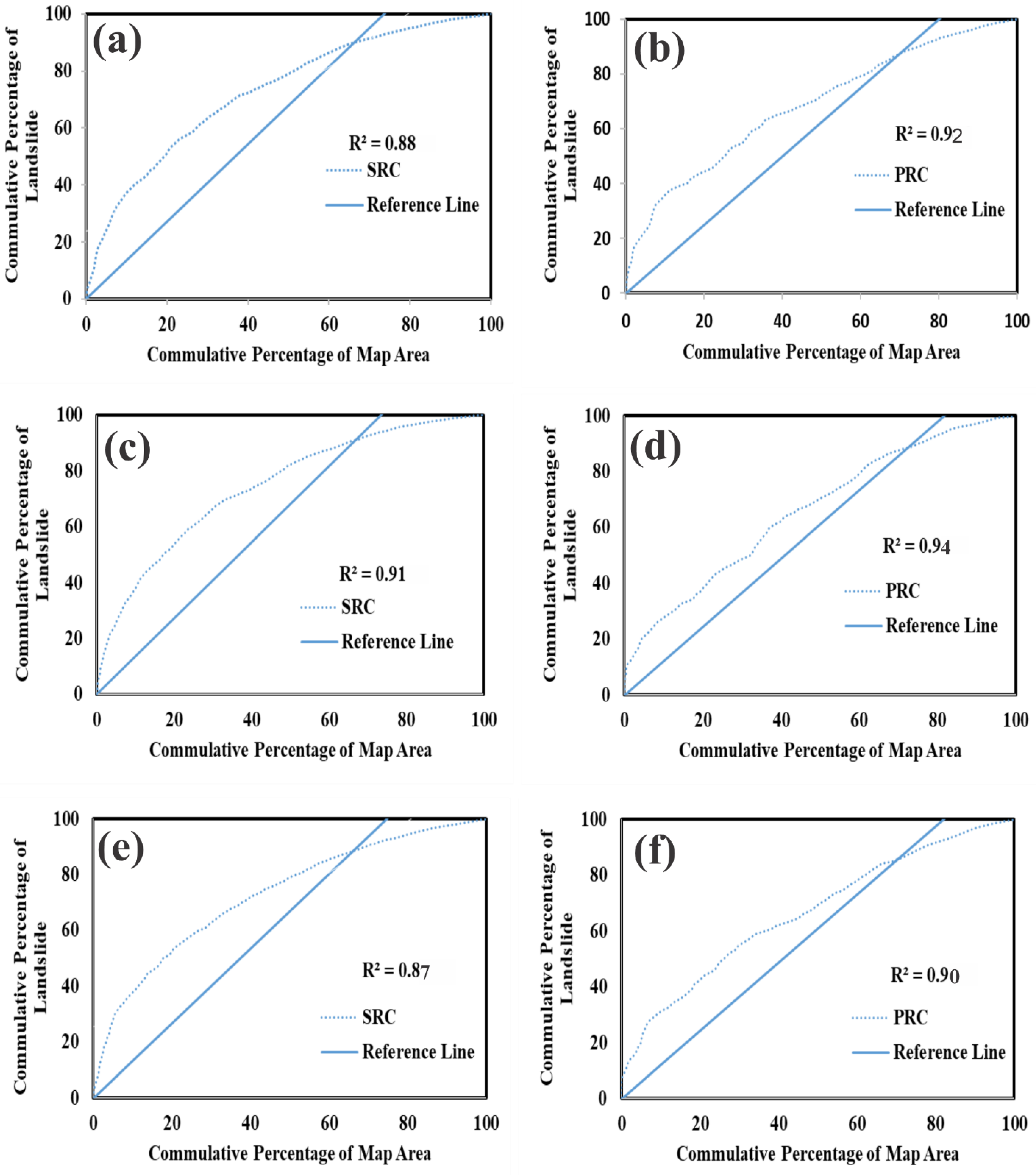
3.2.3. Soil Erosion Susceptibility Mapping Techniques
- (i)
- Weight of Evidence: WOE is a GIS-based quantitative model that uses the Bayes rule to combine data to estimate the likelihood of occurrences [51]. The WOE approach was initially intended to assess mineral potential mapping using geospatial modelling [52]. The WOE model employs statistical techniques to measure the comparative significance established on the log-linear approach of Bayesian probability. In the case of the WOE model, the positive (W+) and negative (W−) weights are identified as the most important components. The weight of both causative parameters (B) established on the existence or non-existence of soil erosion (C) of research area is evaluated [53] using the equations below.
- (ii)
- Frequency Ration (FR): The FR model has been widely considered as one of the most effective GIS-based models for determining the spatial relationship between two variables [56]. This methodology is a fairly consistent experimental method for producing LSM for the investigated area [57]. The 2.12 algorithm was used to calculate the FR for each predisposing parameter.where FR is the Frequency Ratio, NiPx is the number of pixels in each landslide conditioning factor class, N is the total number of pixels in the study area, NilP is the number of landslide pixels in each landslide conditioning factor, and Nl is the total number of landslide pixels in the study area. To create LSI for the area of interest, the following mathematical algorithm was used.
- (iii)
- Information Value: This approach was used in the current study to generate LSM of the research region. This model, which is based on GIS and RS, was used to forecast the geographical connection between landslide inventory and several types of predisposing variables [57]. The following computation formula was used to do this evaluation.
4. Results
5. Discussion
6. Conclusions
Author Contributions
Funding
Institutional Review Board Statement
Informed Consent Statement
Data Availability Statement
Conflicts of Interest
References
- Alexakis, D.E.; Bathrellos, G.D.; Skilodimou, H.D.; Gamvroula, D.E. Spatial Distribution and Evaluation of Arsenic and Zinc Content in the Soil of a Karst Landscape. Sustainability 2021, 13, 6976. [Google Scholar] [CrossRef]
- Alexakis, D.E.; Bathrellos, G.D.; Skilodimou, H.D.; Gamvroula, D.E. Land Suitability Mapping Using Geochemical and Spatial Analysis Methods. Appl. Sci. 2021, 11, 5404. [Google Scholar] [CrossRef]
- Band, S.S.; Janizadeh, S.; Chandra Pal, S.; Saha, A.; Chakrabortty, R.; Shokri, M.; Mosavi, A. Novel Ensemble Approach of Deep Learning Neural Network (DLNN) Model and Particle Swarm Optimization (PSO) Algorithm for Prediction of Gully Erosion Susceptibility. Sensors 2020, 20, 5609. [Google Scholar] [CrossRef] [PubMed]
- Arabameri, A.; Asadi Nalivan, O.; Chandra Pal, S.; Chakrabortty, R.; Saha, A.; Lee, S.; Pradhan, B.; Tien Bui, D. Novel Machine Learning Approaches for Modelling the Gully Erosion Susceptibility. Remote Sens. 2020, 12, 2833. [Google Scholar] [CrossRef]
- Puente, C.; Olague, G.; Trabucchi, M.; Arjona-Villicaña, P.D.; Soubervielle-Montalvo, C. Synthesis of Vegetation Indices Using Genetic Programming for Soil Erosion Estimation. Remote Sens. 2019, 11, 156. [Google Scholar] [CrossRef]
- Ochoa, P.a.a.; Fries, A.; Mejía, D.; Burneo, J.; Ruíz-Sinoga, J.; Cerdà, A. Effects of climate, land cover and topography on soil erosion risk in a semiarid basin of the Andes. Catena 2016, 140, 31–42. [Google Scholar] [CrossRef]
- Panagos, P.; Borrelli, P.; Meusburger, K. A new European slope length and steepness factor (LS-Factor) for modeling soil erosion by water. Geosciences 2015, 5, 117–126. [Google Scholar] [CrossRef]
- Sun, W.; Shao, Q.; Liu, J.; Zhai, J. Assessing the effects of land use and topography on soil erosion on the Loess Plateau in China. Catena 2014, 121, 151–163. [Google Scholar] [CrossRef]
- Xu, C.Y.; Chen, D. Comparison of seven models for estimation of evapotranspiration and groundwater recharge using lysimeter measurement data in Germany. Hydrol. Process. Int. J. 2005, 19, 3717–3734. [Google Scholar] [CrossRef]
- Brunner, A.; Park, S.; Ruecker, G.; Dikau, R.; Vlek, P. Catenary soil development influencing erosion susceptibility along a hillslope in Uganda. Catena 2004, 58, 1–22. [Google Scholar] [CrossRef]
- Veihe, A. Sustainable Farming Practices: Ghanaian Farmers’ Perception of Erosion and Their Use of Conservation Measures. Environ. Manag. 2000, 25, 393–402. [Google Scholar] [CrossRef] [PubMed]
- Jaafari, A.; Najafi, A.; Pourghasemi, H.R.; Rezaeian, J.; Sattarian, A. GIS-based frequency ratio and index of entropy models for landslide susceptibility assessment in the Caspian forest, northern Iran. Int. J. Environ. Sci. Technol. 2014, 11, 909–926. [Google Scholar] [CrossRef]
- Kiani-Harchegani, M.; Najafi, S.; Ghahramani, A. Chapter 18-Measuring and mapping excessive linear soil erosion features: Rills and gullies. In Precipitation; Rodrigo-Comino, J., Ed.; Elsevier: Amsterdam, The Netherlands, 2021; pp. 419–438. [Google Scholar]
- Ligonja, P.J.; Shrestha, R.P. Soil Erosion Assessment in Kondoa Eroded Area in Tanzania using Universal Soil Loss Equation, Geographic Information Systems and Socioeconomic Approach. Land Degrad. Dev. 2015, 26, 367–379. [Google Scholar] [CrossRef]
- Galati, A.; Gristina, L.; Crescimanno, M.; Barone, E.; Novara, A. Towards More Efficient Incentives for Agri-environment Measures in Degraded and Eroded Vineyards. Land Degrad. Dev. 2015, 26, 557–564. [Google Scholar] [CrossRef]
- Alam, M.; Hussain, R.R.; Islam, A.B.M.S. Impact assessment of rainfall-vegetation on sedimentation and predicting erosion-prone region by GIS and RS. Geomat. Nat. Hazards Risk 2016, 7, 667–679. [Google Scholar] [CrossRef]
- Khan, J.; Ahmed, W.; Yasir, M.; Islam, I.; Janjuhah, H.T.; Kontakiotis, G. Pollutants Concentration during the Construction and Operation Stages of a Long Tunnel: A Case Study of Lowari Tunnel, (Dir–Chitral), Khyber Pakhtunkhwa, Pakistan. Appl. Sci. 2022, 12, 6170. [Google Scholar] [CrossRef]
- Bathrellos, G.D.; Skilodimou, H.D. Land Use Planning for Natural Hazards. Land 2019, 8, 128. [Google Scholar] [CrossRef]
- Skilodimou, H.D.; Bathrellos, G.D. Natural and Technological Hazards in Urban Areas: Assessment, Planning and Solutions. Sustainability 2021, 13, 8301. [Google Scholar] [CrossRef]
- Valkanou, K.; Karymbalis, E.; Bathrellos, G.; Skilodimou, H.; Tsanakas, K.; Papanastassiou, D.; Gaki-Papanastassiou, K. Soil Loss Potential Assessment for Natural and Post-Fire Conditions in Evia Island, Greece. Geosciences 2022, 12, 367. [Google Scholar] [CrossRef]
- Iqbal, M.F.; Khan, I.A. Spatiotemporal Land Use Land Cover change analysis and erosion risk mapping of Azad Jammu and Kashmir, Pakistan. Egypt. J. Remote Sens. Space Sci. 2014, 17, 209–229. [Google Scholar] [CrossRef]
- Ali, S.A.; Hagos, H. Estimation of soil erosion using USLE and GIS in Awassa Catchment, Rift valley, Central Ethiopia. Geoderma Reg. 2016, 7, 159–166. [Google Scholar] [CrossRef]
- Alewell, C.; Borrelli, P.; Meusburger, K.; Panagos, P. Using the USLE: Chances, challenges and limitations of soil erosion modelling. Int. Soil Water Conserv. Res. 2019, 7, 203–225. [Google Scholar] [CrossRef]
- Sinha, D.; Joshi, V.U. Application of Universal Soil Loss Equation (USLE) to recently reclaimed badlands along the Adula and Mahalungi Rivers, Pravara Basin, Maharashtra. J. Geol. Soc. India 2012, 80, 341–350. [Google Scholar] [CrossRef]
- Abdulkadir, T.S.; Muhammad, R.U.M.; Wan Yusof, K.; Ahmad, M.H.; Aremu, S.A.; Gohari, A.; Abdurrasheed, A.S. Quantitative analysis of soil erosion causative factors for susceptibility assessment in a complex watershed. Cogent Eng. 2019, 6, 1594506. [Google Scholar] [CrossRef]
- Rahman, M.R.; Shi, Z.; Chongfa, C. Soil erosion hazard evaluation—An integrated use of remote sensing, GIS and statistical approaches with biophysical parameters towards management strategies. Ecol. Model. 2009, 220, 1724–1734. [Google Scholar] [CrossRef]
- Akgün, A.; Türk, N. Mapping erosion susceptibility by a multivariate statistical method: A case study from the Ayvalık region, NW Turkey. Comput. Geosci. 2011, 37, 1515–1524. [Google Scholar] [CrossRef]
- Conoscenti, C.; Angileri, S.; Cappadonia, C.; Rotigliano, E.; Agnesi, V.; Märker, M. Gully erosion susceptibility assessment by means of GIS-based logistic regression: A case of Sicily (Italy). Geomorphology 2014, 204, 399–411. [Google Scholar] [CrossRef]
- Mendicino, G. Sensitivity analysis on GIS procedures for the estimate of soil erosion risk. Nat. Hazards 1999, 20, 231–253. [Google Scholar] [CrossRef]
- Dube, F.; Nhapi, I.; Murwira, A.; Gumindoga, W.; Goldin, J.; Mashauri, D. Potential of weight of evidence modelling for gully erosion hazard assessment in Mbire District–Zimbabwe. Phys. Chem. Earth Parts A/B/C 2014, 67, 145–152. [Google Scholar] [CrossRef]
- Magliulo, P. Assessing the susceptibility to water-induced soil erosion using a geomorphological, bivariate statistics-based approach. Environ. Earth Sci. 2012, 67, 1801–1820. [Google Scholar] [CrossRef]
- Mitasova, H.; Hofierka, J.; Zlocha, M.; Iverson, L.R. Modelling topographic potential for erosion and deposition using GIS. Int. J. Geogr. Inf. Syst. 1996, 10, 629–641. [Google Scholar] [CrossRef]
- Gournellos, T.; Evelpidou, N.; Vassilopoulos, A. Developing an Erosion risk map using soft computing methods (case study at Sifnos island). Nat. Hazards 2004, 31, 63–83. [Google Scholar] [CrossRef]
- Conforti, M.; Aucelli, P.P.; Robustelli, G.; Scarciglia, F. Geomorphology and GIS analysis for mapping gully erosion susceptibility in the Turbolo stream catchment (Northern Calabria, Italy). Nat. Hazards 2011, 56, 881–898. [Google Scholar] [CrossRef]
- Lucà, F.; Conforti, M.; Robustelli, G. Comparison of GIS-based gullying susceptibility mapping using bivariate and multivariate statistics: Northern Calabria, South Italy. Geomorphology 2011, 134, 297–308. [Google Scholar] [CrossRef]
- He, D. Modeling of dominating factors to soil and water conservation. Fujian For. Colloid Trans. 1999, 19, 26–29. [Google Scholar]
- Kausar, R.; Baig, S.; Riaz, I. Spatio-Temporal Land Use/Land Cover Analysis of Murree using Remote Sensing and GIS. Asian J. Agric. Rural Dev. 2016, 6, 50–58. [Google Scholar] [CrossRef]
- Jamal, T.; Naseer, S.; Shehzad Hassan, S.; Batool, H.; Mahmood, R.; Naz, A.; Butt, A.; Tanver, U.; Saddique Kaukab, I.; Alvi, S.; et al. Appraisal of Deforestation in Murree through Open Source Satellite Imagery. Adv. Remote Sens. 2018, 7, 61–70. [Google Scholar] [CrossRef]
- Virk, Z.T.; Khalid, B.; Hussain, A.; Ahmad, B.; Dogar, S.S.; Raza, N.; Iqbal, B. Water availability, consumption and sufficiency in Himalayan towns: A case of Murree and Havellian towns from Indus River Basin, Pakistan. Water Policy 2019, 22, 46–64. [Google Scholar] [CrossRef]
- Zeitler, P.K. Cooling history of the NW Himalaya, Pakistan. Tectonics 1985, 4, 127–151. [Google Scholar] [CrossRef]
- Abbasi, A.; Khan, M.A.; Ishfaq, M.; Mool, P.K. Slope failure and landslide mechanism in Murree area, North Pakistan. Geol. Bull. Univ. Peshawar 2002, 35, 125–137. [Google Scholar]
- Al-Abadi, A.M. Mapping flood susceptibility in an arid region of southern Iraq using ensemble machine learning classifiers: A comparative study. Arab. J. Geosci. 2018, 11, 218. [Google Scholar] [CrossRef]
- Chalise, D.; Kumar, L.; Kristiansen, P. Land Degradation by Soil Erosion in Nepal: A Review. Soil Syst. 2019, 3, 12. [Google Scholar] [CrossRef]
- Holz, D.J.; Williard, K.W.J.; Edwards, P.J.; Schoonover, J.E. Soil Erosion in Humid Regions: A Review. J. Contemp. Water Res. Educ. 2015, 154, 48–59. [Google Scholar] [CrossRef]
- Perreault, L.M.; Yager, E.M.; Aalto, R. Effects of gradient, distance, curvature and aspect on steep burned and unburned hillslope soil erosion and deposition. Earth Surf. Processes Landf. 2017, 42, 1033–1048. [Google Scholar] [CrossRef]
- Meng, X.; Zhu, Y.; Yin, M.; Liu, D. The impact of land use and rainfall patterns on the soil loss of the hillslope. Sci. Rep. 2021, 11, 16341. [Google Scholar] [CrossRef] [PubMed]
- Hailemariam, S.N.; Soromessa, T.; Teketay, D. Land Use and Land Cover Change in the Bale Mountain Eco-Region of Ethiopia during 1985 to 2015. Land 2016, 5, 41. [Google Scholar] [CrossRef]
- Aslam, B.; Maqsoom, A.; Salah Alaloul, W.; Ali Musarat, M.; Jabbar, T.; Zafar, A. Soil erosion susceptibility mapping using a GIS-based multi-criteria decision approach: Case of district Chitral, Pakistan. Ain Shams Eng. J. 2021, 12, 1637–1649. [Google Scholar] [CrossRef]
- Ayalew, D.A.; Deumlich, D.; Šarapatka, B.; Doktor, D. Quantifying the Sensitivity of NDVI-Based C Factor Estimation and Potential Soil Erosion Prediction using Spaceborne Earth Observation Data. Remote Sens. 2020, 12, 1136. [Google Scholar] [CrossRef]
- Lee, S. Soil erosion assessment and its verification using the Universal Soil Loss Equation and Geographic Information System: A case study at Boun, Korea. Environ. Geol. 2004, 45, 457–465. [Google Scholar] [CrossRef]
- Elmoulat, M.; Ait Brahim, L.; Mastere, M.; Ilham Jemmah, A. Mapping of Mass Movements Susceptibility in the Zoumi Region Using Satellite Image and GIS Technology (Moroccan Rif). Int. J. Sci. Eng. Res. 2015, 6, 210–217. [Google Scholar]
- Bonham-Carter, G.F.; Agterberg, F.P.; Wright, D.F. Integration of Geological Datasets for Gold Exploration in Nova Scotia. In Digital Geologic and Geographic Information Systems; Short Courses in Geology; Wiley: New York, NY, USA, 1989; pp. 15–23. [Google Scholar]
- Bonham-Carter, G.F. Geographic Information Systems for Geoscientists: Modelling with GIS; Elsevier: Amsterdam, The Netherlands, 1994; Volume 13. [Google Scholar]
- Xu, C.; Xu, X.; Dai, F.; Xiao, J.; Tan, X.; Yuan, R. Landslide hazard mapping using GIS and weight of evidence model in Qingshui River watershed of 2008 Wenchuan earthquake struck region. J. Earth Sci. 2012, 23, 97–120. [Google Scholar] [CrossRef]
- Dahal, R.K.; Hasegawa, S.; Nonomura, A.; Yamanaka, M.; Dhakal, S.; Paudyal, P. Predictive modelling of rainfall-induced landslide hazard in the Lesser Himalaya of Nepal based on weights-of-evidence. Geomorphology 2008, 102, 496–510. [Google Scholar] [CrossRef]
- Oh, H.-J.; Lee, S.; Hong, S.-M. Landslide Susceptibility Assessment Using Frequency Ratio Technique with Iterative Random Sampling. J. Sens. 2017, 2017, 1–21. [Google Scholar] [CrossRef]
- Fayez, L.; Pazhman, D.; Thai Pham, B.; Dholakia, M.B.; Solanki, H.A.; Khalid, M.A.; Prakash, I. Application of Frequency Ratio Model for the Development of Landslide Susceptibility Mapping at Part of Uttarakhand State, India. Int. J. Appl. Eng. Res. 2018, 13, 6846–6854. [Google Scholar]
- Safriel, U. Land Degradation Neutrality (LDN) in Drylands and Beyond–Where has it come from and where does it go. Silva Fenn. 2017, 51, 1650. [Google Scholar] [CrossRef]
- Dooley, E.; Roberts, E.; Wunder, S. Land degradation neutrality under the SDGs: National and international implementation of the land degradation neutral world target. Elni Rev. 2015, 1, 2–9. [Google Scholar] [CrossRef]
- Pradeep, G.S.; Krishnan, M.V.N.; Vijith, H. Identification of critical soil erosion prone areas and annual average soil loss in an upland agricultural watershed of Western Ghats, using analytical hierarchy process (AHP) and RUSLE techniques. Arab. J. Geosci. 2015, 8, 3697–3711. [Google Scholar] [CrossRef]
- Rahmati, O.; Haghizadeh, A.; Pourghasemi, H.R.; Noormohamadi, F. Gully erosion susceptibility mapping: The role of GIS-based bivariate statistical models and their comparison. Nat. Hazards 2016, 82, 1231–1258. [Google Scholar] [CrossRef]
- Arabameri, A.; Rezaei, K.; Pourghasemi, H.R.; Lee, S.; Yamani, M. GIS-based gully erosion susceptibility mapping: A comparison among three data-driven models and AHP knowledge-based technique. Environ. Earth Sci. 2018, 77, 1–22. [Google Scholar] [CrossRef]
- Das, B.; Bordoloi, R.; Thungon, L.T.; Paul, A.; Pandey, P.K.; Mishra, M.; Tripathi, O.P. An integrated approach of GIS, RUSLE and AHP to model soil erosion in West Kameng watershed, Arunachal Pradesh. J. Earth Syst. Sci. 2020, 129, 1–18. [Google Scholar] [CrossRef]
- Sar, N.; Khan, A.; Chatterjee, S.; Das, A.; Mipun, B.S. WITHDRAWN: Coupling of analytical hierarchy process and frequency ratio based spatial prediction of soil erosion susceptibility in Keleghai river basin, India. Int. Soil Water Conserv. Res. 2016. [Google Scholar] [CrossRef]
- Zhou, P.; Luukkanen, O.; Tokola, T.; Nieminen, J. Effect of vegetation cover on soil erosion in a mountainous watershed. Catena 2008, 75, 319–325. [Google Scholar] [CrossRef]
- Agnesi, V.; Angileri, S.; Cappadonia, C.; Conoscenti, C.; Rotigliano, E. Multi parametric gis analysis to assess gully erosion susceptibility: A test in southern sicily, italy. Landf. Anal. 2011, 17, 15–20. [Google Scholar]
- Islam, F.; Riaz, S.; Ghaffar, B.; Tariq, A.; Shah, S.U.; Nawaz, M.; Hussain, M.L.; Amin, N.U.; Li, Q.; Lu, L.; et al. Landslide susceptibility mapping (LSM) of Swat District, Hindu Kush Himalayan region of Pakistan, using GIS-based bivariate modeling. Front. Environ. Sci. 2022, 10, 1–18. [Google Scholar] [CrossRef]


| Data | Scale/Resolution | Availability of Data | Data availability Statement/Source | Parameter Maps |
|---|---|---|---|---|
| Sentinel -2 | 10 m | Data openly available | The data supporting this study’s findings are openly available in [USGS] at https://earthexplorer.usgs.gov (accessed on 1 July 2022). The spatial resolution is 30 m. | Land Use Land Cover |
| SRTM DEM | 30 m | Data openly available | The data that support the findings of this study are openly available in [USGS] at https://earthexplorer.usgs.gov (accessed on 5 July 2022) Spatial resolution is 30 m. | Elevation, Slope, Aspect, Curvature, and drainage |
| CHIRPS | 0.05° | Data openly available | The data supporting this study’s findings are available in [UCSB] at https://www.chc.ucsb.edu (accessed on 30 July 2022). The spatial resolution of CHIPRS is 0.05° (5.54 Km) and daily gridded. | Rainfall maps |
| Soil | 1:2,000,000 | Soil Survey of Pakistan | The data available from FAO and Soil Survey of Pakistan | Soil Texture Map |
| Geology | 1:650,000 | (Searle et al.) | Digitized from Geological Map of North Pakistan | Lithological Map |
| Sentinel 2 | 10 m | Data openly available | Data import to GEE using machine learning algorithm. | NDVI Map and soil erosion inventory |
| Parameters | Class | No of Pixels in Class | No of Landslide Pixels in A Class | W+ | W− | WoE | % Pixels in Class | % LS Pixels in Class | (FR) | IV = log (A/B) |
|---|---|---|---|---|---|---|---|---|---|---|
| Elevation | <900 | 107,632 | 422 | −1.41 | 0.20 | −1.6 | 22.46 | 5.52 | 0.24 | −1.40 |
| 900–1100 | 71,920 | 900 | −0.24 | 0.03 | −0.28 | 15.01 | 11.78 | 0.78 | −0.24 | |
| 1100–1300 | 85,410 | 1216 | −0.11 | 0.02 | −0.13 | 17.82 | 15.92 | 0.89 | −0.11 | |
| 1300–1500 | 72,886 | 2800 | 0.90 | −0.29 | 1.50 | 15.21 | 36.65 | 2.36 | 1.51 | |
| >1500 | 141,251 | 2300 | 0.02 | −0.00 | 0.03 | 29.48 | 30.11 | 1.021 | 0.021 | |
| Slope | <10 | 60,344 | 799 | 0.60 | −0.12 | 0.73 | 12.70 | 10.46 | 0.82 | 0.59 |
| 10–20 | 217,254 | 3200 | 0.71 | −1.97 | 2.68 | 45.73 | 41.89 | 0.91 | 0.70 | |
| 20–30 | 165,432 | 2940 | 0.90 | −1.46 | 2.36 | 34.82 | 38.49 | 1.10 | 0.89 | |
| 30–40 | 30,547 | 648 | 1.08 | −0.14 | 1.22 | 6.43 | 8.48 | 1.31 | 1.06 | |
| >40 | 1461 | 51 | 1.52 | −0.01 | 1.53 | 0.30 | 0.66 | 2.40 | 1.52 | |
| Aspect | F | 36,821 | 572 | −0.02 | 0.00 | −0.03 | 7.75 | 5.94 | 0.76 | −0.26 |
| NE | 34,546 | 1201 | −0.03 | 0.00 | −0.03 | 7.75 | 7.49 | 0.97 | −0.14 | |
| E | 52,413 | 509 | 0.80 | −0.10 | 0.89 | 7.27 | 15.72 | 2.16 | 0.41 | |
| SE | 74,371 | 542 | −0.51 | 0.05 | −0.55 | 11.03 | 6.66 | 0.60 | 0.44 | |
| S | 63,720 | 2243 | −0.80 | 0.10 | −0.89 | 15.66 | 7.10 | 0.45 | −2.04 | |
| SW | 42,743 | 817 | 0.81 | −0.21 | 1.02 | 13.41 | 29.37 | 2.19 | 1.198 | |
| W | 47,930 | 640 | 0.18 | −0.02 | 0.20 | 9.00 | 10.70 | 1.19 | 0.19 | |
| NW | 61,501 | 388 | −0.18 | 0.02 | −0.20 | 10.09 | 8.38 | 0.83 | 0.42 | |
| N | 60,993 | 688 | −0.94 | 0.09 | −1.03 | 12.95 | 5.08 | 0.39 | −0.24 | |
| Curvature | Concave | 118,738 | 4170 | 0.81 | −0.51 | 1.32 | 24.78 | 54.60 | 2.20 | 0.97 |
| Flat | 262,259 | 962 | −1.48 | 0.67 | −2.16 | 54.74 | 12.59 | 0.23 | −1.47 | |
| Convex | 98,102 | 2506 | 0.48 | −0.17 | 0.65 | 20.48 | 32.8 | 1.60 | 0.47 | |
| Distance to Stream | <25 | 6968 | 775 | 1.66 | −0.09 | 1.87 | 2.05 | 6.45 | 3.01 | 1.60 |
| 25–50 | 9840 | 493 | 1.55 | −0.05 | 1.60 | 3.77 | 14.94 | 2.87 | 1.49 | |
| 50–100 | 18,071 | 1141 | 1.4 | −0.13 | 1.55 | 1.45 | 10.15 | 1.97 | 1.38 | |
| 100–250 | 47,475 | 1447 | 0.66 | −0.11 | 0.77 | 9.91 | 18.94 | 0.93 | 0.65 | |
| >250 | 396,744 | 3782 | −0.52 | 1.11 | −1.63 | 82.81 | 49.52 | 0.60 | −1.05 | |
| Precipitation (mm/year) | 1410–1571 | 47,185 | 332 | −0.84 | 0.06 | −0.90 | 9.93 | 4.35 | 0.44 | −0.83 |
| 1571–1681 | 98,970 | 972 | −0.50 | 0.10 | −0.60 | 20.83 | 12.73 | 0.61 | −0.49 | |
| 1681–1773 | 94,900 | 1041 | −0.39 | 0.08 | −0.47 | 19.98 | 13.63 | 0.68 | −0.38 | |
| 1773–1881 | 72,489 | 1042 | −0.11 | 0.02 | −0.13 | 15.26 | 13.64 | 0.89 | −0.11 | |
| 1881–2035 | 161,494 | 4251 | 0.50 | −0.40 | 1.57 | 34.00 | 55.66 | 2.98 | 1.58 | |
| LULC | Forest | 210,650 | 2000 | −0.52 | 0.28 | −0.81 | 43.97 | 26.18 | 0.50 | −0.52 |
| Vegetation | 141,362 | 2327 | 0.03 | −0.01 | 0.05 | 29.50 | 30.47 | 0.73 | 0.03 | |
| Barren Land | 63,576 | 2010 | 0.70 | 1.54 | 0.93 | 13.27 | 26.32 | 2.46 | 1.53 | |
| Urban | 61,743 | 200 | −1.61 | 0.11 | −1.72 | 12.89 | 2.62 | 0.20 | −1.59 | |
| Water | 1796 | 10 | −1.06 | 0.00 | −1.06 | 0.37 | 0.13 | 0.35 | −0.95 | |
| Lithology | Alluvium | 1269 | 17 | −0.18 | 0.00 | −0.18 | 0.26 | 0.22 | 0.84 | −0.17 |
| Quaternary | 18,192 | 263 | 0.24 | −0.01 | 0.25 | 2.71 | 3.44 | 1.27 | 0.24 | |
| Muree Formation | 398,228 | 6686 | 0.04 | −0.22 | 0.26 | 84.58 | 87.54 | 1.03 | 0.04 | |
| Kuldana | 20,835 | 379 | 0.14 | −0.01 | 0.14 | 4.35 | 4.96 | 1.14 | 0.13 | |
| Lora | 10,620 | 73 | −0.85 | 0.01 | −0.86 | 2.22 | 0.96 | 0.43 | −0.84 | |
| Margalla Hill Limestone | 6774 | 177 | −0.89 | 0.03 | −0.92 | 5.59 | 2.32 | 0.41 | −0.88 | |
| Kuzagali Shale | 683 | 27 | 0.93 | 0.00 | 1.553 | 0.14 | 0.35 | 2.48 | 1.56 | |
| Mari Limestone | 697 | 10 | −0.11 | 0.00 | −0.11 | 0.15 | 0.13 | 0.90 | −0.10 | |
| Fault Buffer | <25 | 2468 | 30 | −0.28 | 0.00 | −0.28 | 0.52 | 0.39 | 0.76 | −0.27 |
| 25–50 | 4000 | 63 | −0.24 | 0.00 | −0.24 | 1.04 | 0.82 | 0.79 | −0.24 | |
| 50–100 | 7488 | 94 | −0.24 | 0.00 | −0.25 | 1.56 | 1.23 | 0.79 | −0.24 | |
| 100–250 | 18,894 | 377 | 0.18 | −0.01 | 0.18 | 4.15 | 4.94 | 1.19 | 0.17 | |
| >250 | 446,248 | 7074 | 0.00 | 0.02 | −0.02 | 92.73 | 92.62 | 1.00 | 0.00 | |
| Soil | Loamy and Clayey non-calcareous soil | 292,459 | 2538 | −0.67 | 0.64 | −1.30 | 64.17 | 33.23 | 0.73 | −0.66 |
| Loamy and non-calcareous soil | 186,639 | 5101 | 0.64 | −0.67 | 1.55 | 35.83 | 66.78 | 2.79 | 1.56 | |
| NDVI | Low | 98,102 | 3306 | 0.76 | −0.34 | 1.10 | 20.65 | 43.28 | 2.43 | 1.52 |
| Medium | 262,259 | 3670 | −0.13 | 0.14 | 1.46 | 55.21 | 48.05 | 1.53 | 1.47 | |
| High | 118,738 | 662 | −1.06 | 0.19 | −1.25 | 25.00 | 8.67 | 0.05 | −0.9 | |
| Distance to Road | <20 | 6437 | 92 | 0.68 | −0.01 | 0.69 | 1.34 | 0.63 | 1.53 | 0.67 |
| 20–40 | 6401 | 64 | 0.32 | −0.005 | 0.32 | 1.33 | 0.51 | 1.37 | 0.31 | |
| 40–100 | 18,535 | 157 | 0.15 | −0.006 | 0.16 | 3.86 | 1.55 | 1.16 | 0.15 | |
| 100–350 | 67,753 | 516 | 0.04 | −0.008 | 0.05 | 14.14 | 3.93 | 1.04 | 0.04 | |
| >350 | 379,972 | 2650 | −0.04 | 0.14 | −0.18 | 79.30 | 93.36 | 0.96 | −0.04 |
Publisher’s Note: MDPI stays neutral with regard to jurisdictional claims in published maps and institutional affiliations. |
© 2022 by the authors. Licensee MDPI, Basel, Switzerland. This article is an open access article distributed under the terms and conditions of the Creative Commons Attribution (CC BY) license (https://creativecommons.org/licenses/by/4.0/).
Share and Cite
Islam, F.; Ahmad, M.N.; Janjuhah, H.T.; Ullah, M.; Islam, I.U.; Kontakiotis, G.; Skilodimou, H.D.; Bathrellos, G.D. Modelling and Mapping of Soil Erosion Susceptibility of Murree, Sub-Himalayas Using GIS and RS-Based Models. Appl. Sci. 2022, 12, 12211. https://doi.org/10.3390/app122312211
Islam F, Ahmad MN, Janjuhah HT, Ullah M, Islam IU, Kontakiotis G, Skilodimou HD, Bathrellos GD. Modelling and Mapping of Soil Erosion Susceptibility of Murree, Sub-Himalayas Using GIS and RS-Based Models. Applied Sciences. 2022; 12(23):12211. https://doi.org/10.3390/app122312211
Chicago/Turabian StyleIslam, Fakhrul, Muhammad Nasar Ahmad, Hammad Tariq Janjuhah, Matee Ullah, Ijaz Ul Islam, George Kontakiotis, Hariklia D. Skilodimou, and George D. Bathrellos. 2022. "Modelling and Mapping of Soil Erosion Susceptibility of Murree, Sub-Himalayas Using GIS and RS-Based Models" Applied Sciences 12, no. 23: 12211. https://doi.org/10.3390/app122312211
APA StyleIslam, F., Ahmad, M. N., Janjuhah, H. T., Ullah, M., Islam, I. U., Kontakiotis, G., Skilodimou, H. D., & Bathrellos, G. D. (2022). Modelling and Mapping of Soil Erosion Susceptibility of Murree, Sub-Himalayas Using GIS and RS-Based Models. Applied Sciences, 12(23), 12211. https://doi.org/10.3390/app122312211