

Towards Explainable Quantum Machine Learning for Mobile Malware Detection and Classification †

 ,
,  ,
,
Abstract
1. Introduction
- A fully quantum Machine Learning network is presented and considered in the experimental analysis, while in the previous paper, a quantum hybrid network was considered. The latter represents the main contribution of the paper: in fact, this represents the first attempt to apply a fully quantum Machine Learning model to a malware detection task;
- A comparison between two different quantum architectures, i.e., the full and the hybrid quantum one;
- Comparison between state-of-the-art Convolutional Neural Network and quantum architectures;
- We extend the number of experiments presented in [17] by tuning the models with the aim to empirically obtain better detection performances;
- Three state-of-the-art deep learning models are added (i.e., VGG19, MobileNet, and EfficientNet) to perform a more complete comparison:
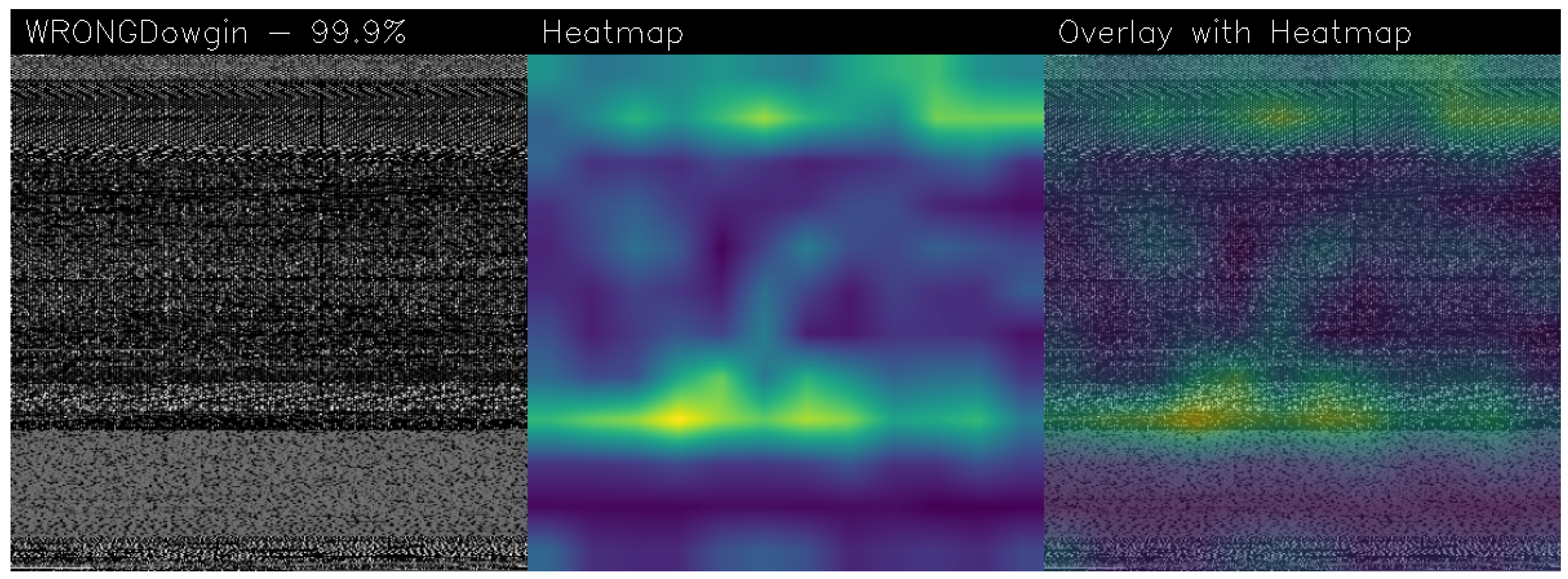
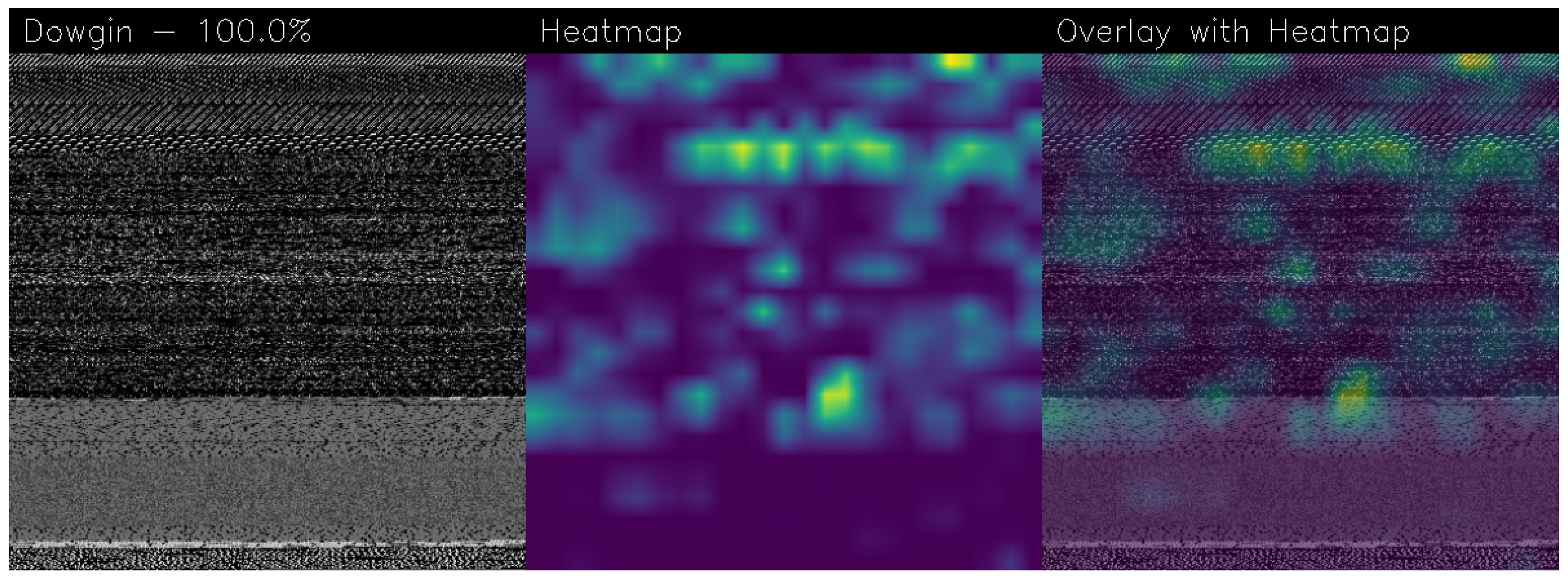
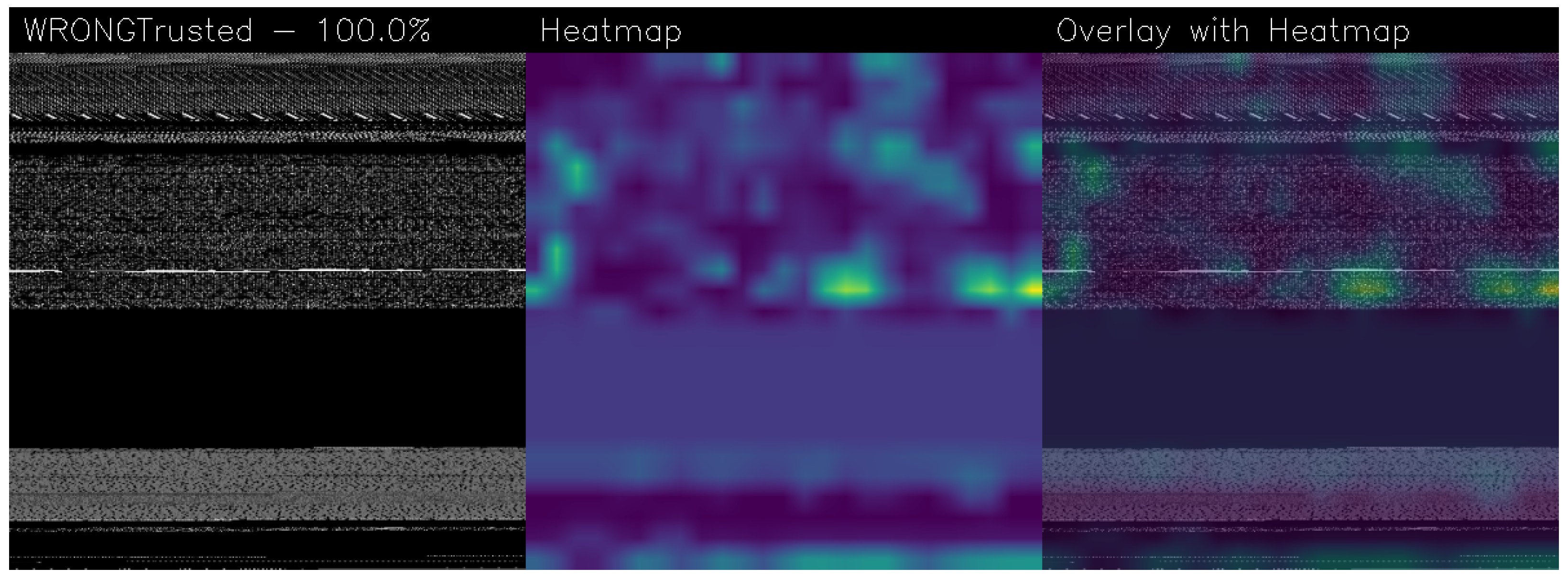
- To provide explainability behind the model decision, we resort to an algorithm aimed to highlight the areas of the application under analysis (represented as an image) that mostly contributed to a certain prediction (i.e., malware or Trusted). To the best of the knowledge of the authors, this is the second main contribution of the paper. Indeed, this is the first attempt to apply explainability to a quantum Machine Learning model;
- We freely release for research purposes the source code we developed for the fully quantum architecture, to encourage researchers to investigate this area.
2. Background
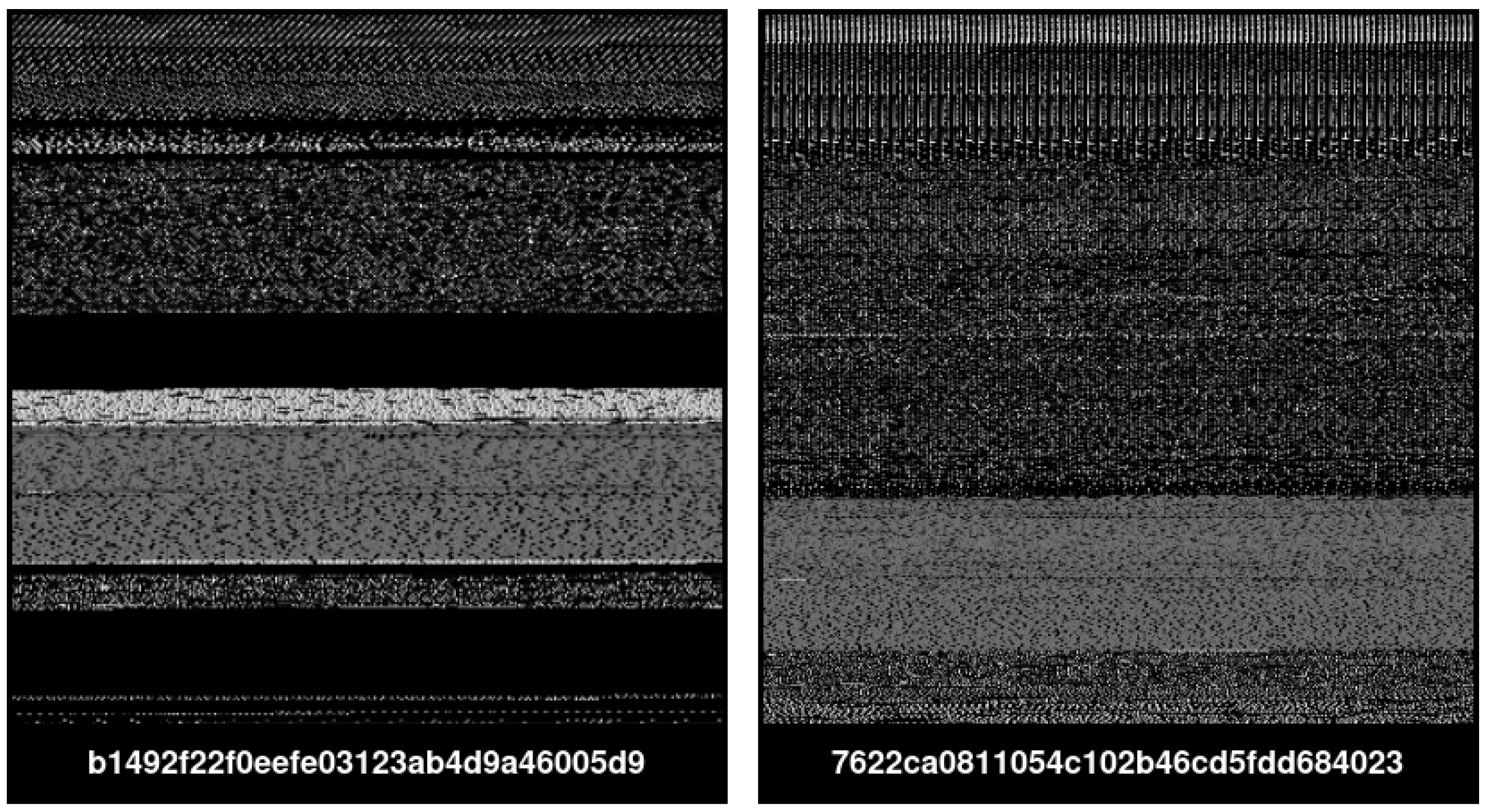
2.1. Image-Based Malware Detection
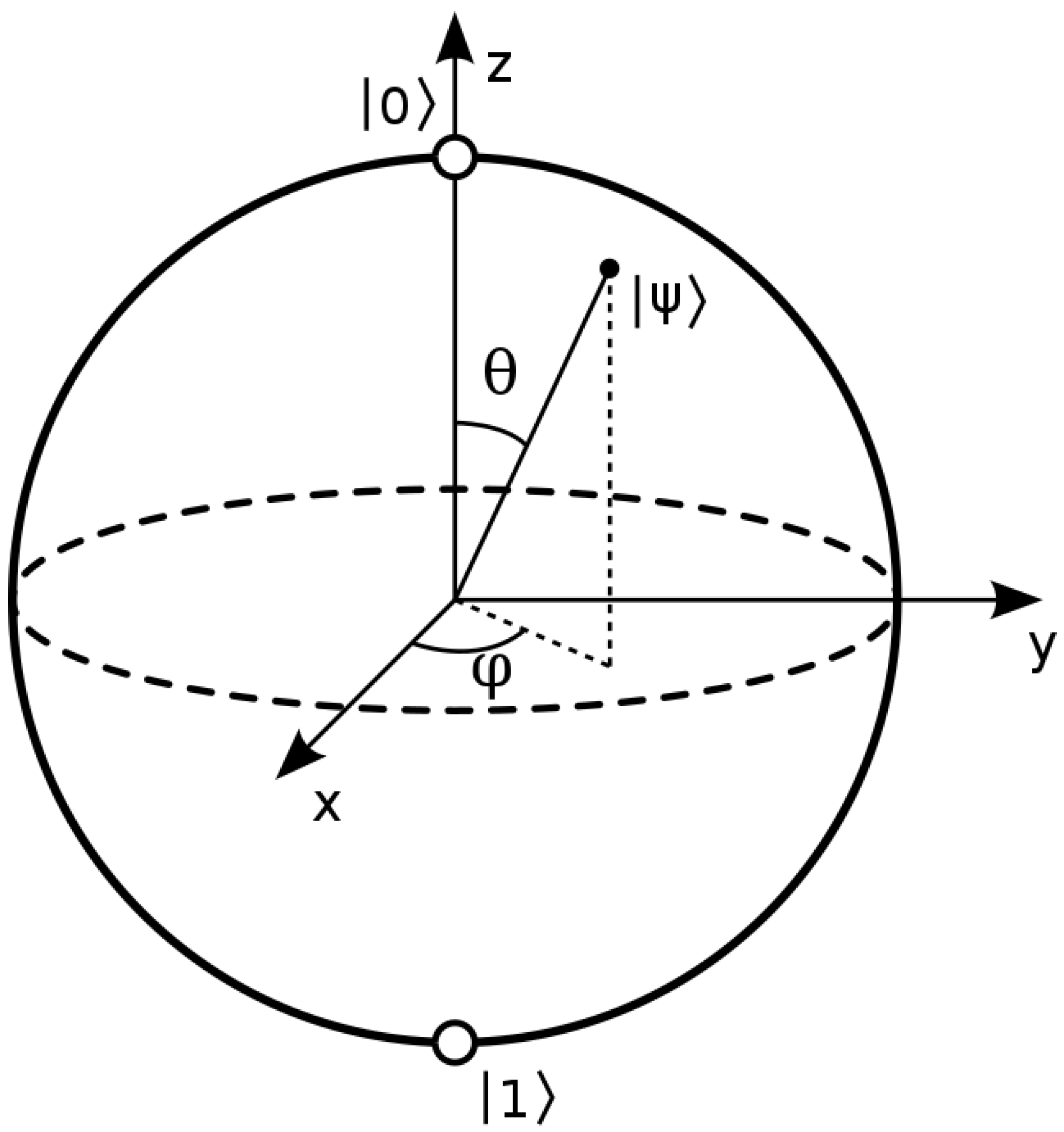
2.2. Quantum Computing
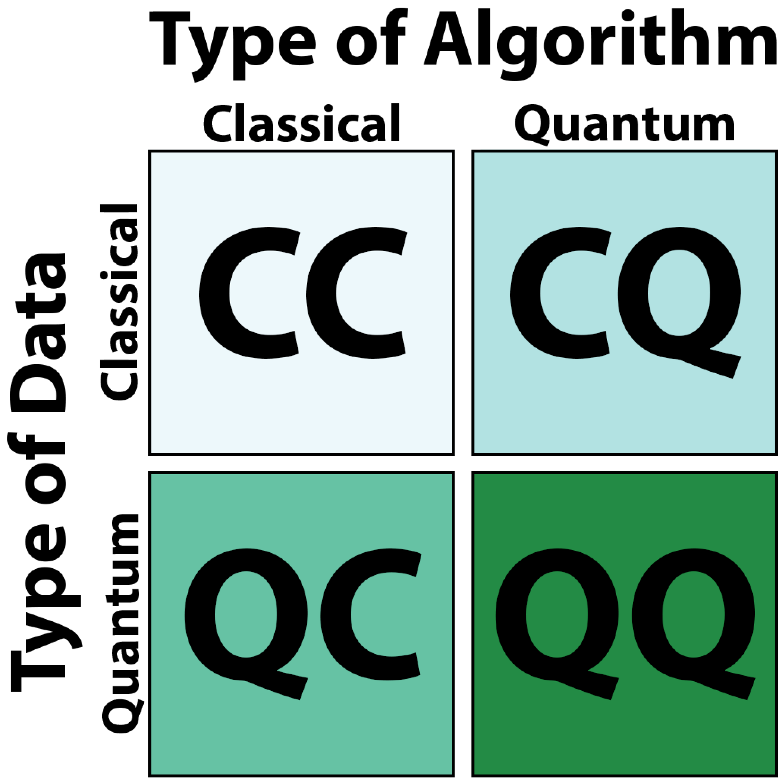
2.3. Quantum and Classical Machine Learning
2.4. Quantum Neural Network
2.5. Grad-CAM
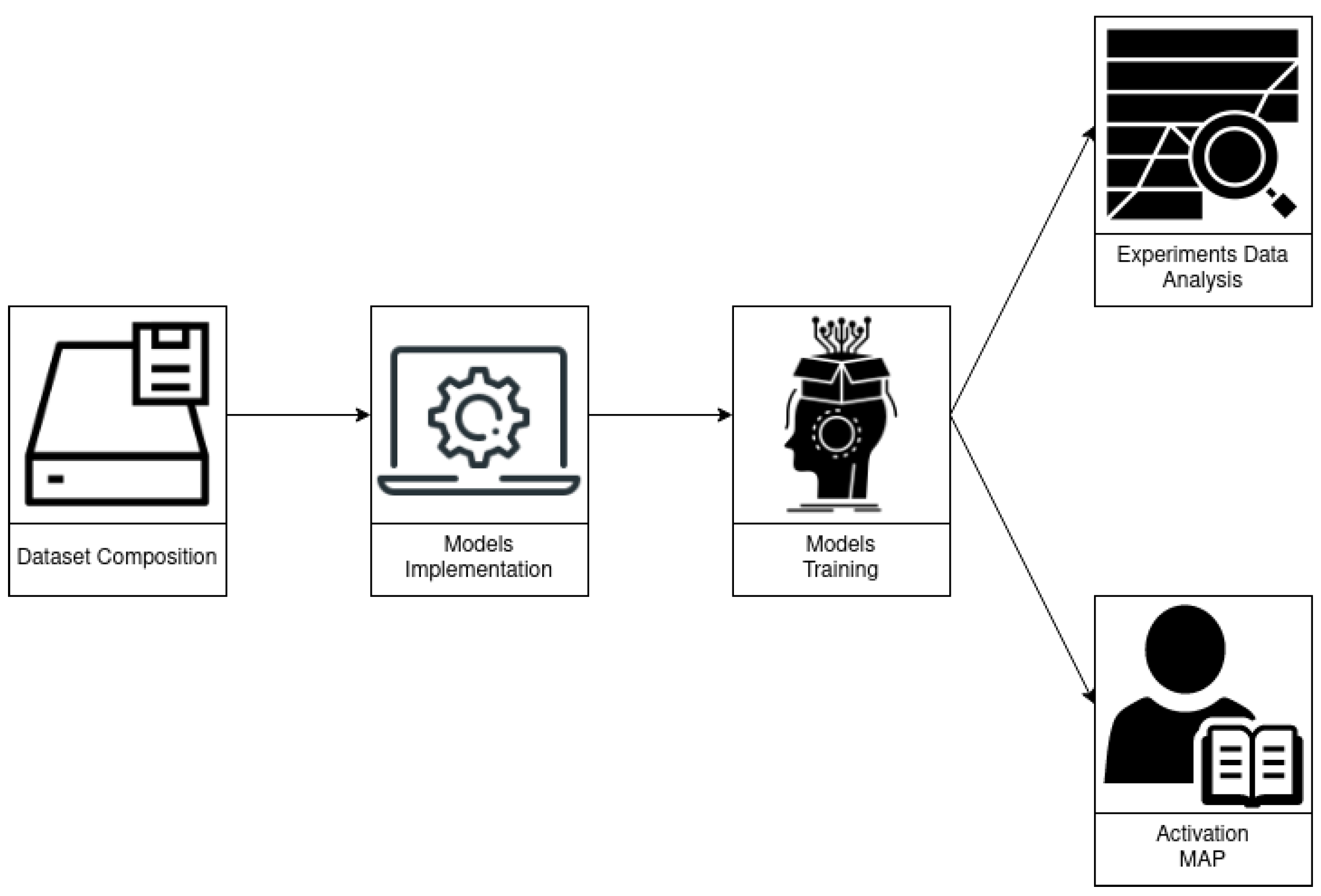
3. Method
3.1. Dataset
3.2. Model Research and Implementation
- Standard-CNN: From 2012, CNNs conquered a plethora of of the ICISSP, 22 gen–24 gen 2018 2018 tasks and are currently growing at a rapid pace. There are differences in their architecture, but all the CNN models are based on the principle of the convolutional filter. This filter, called the kernel, is applied to the pixel matrix that composes the image on the three RGB levels. We report the structure of the CNN proposed by the authors in [17] in Listing 1. The idea is to consider a lighter model if compared to state-of-the-art models (as, for instance, VGG16 also exploited in the comparison). For the Standard-CNN, the following layers (usually considered by typical CNN models) are exploited: convolutional, Maxpooling, Dropout, and Dense layers;
- Visual Geometry Group 16: This network, also known as VGG-16 [33], was designed and developed in 2014 to solve difficult image classification tasks by exploiting ImageNet, an extended dataset composed of 1000 different output labels belonging to different domains. The VGG16 network demonstrated that network depth is a crucial factor to increase classification accuracy in deep learning. The VGG16 model is composed of several convolution layers, each one with a 3 × 3 filter and Maxpooling layers considering a 2 × 2 filter. The 16 in VGG16 is related to the 16 layers with trainable weights in its architecture. The last model part is composed of 2 fully connected (Dense) layers with a softmax activation to perform the classification task. One of the most typical approaches for VGG16’s training is devoted to keeping the convolutional part of the model with the weights obtained from training the model on the ImageNet dataset, while the Dense layers part is trained for the specific classification task required;
- Visual Geometry Group 19: Also known as VGG19, it was introduced by Oxford University following VGG16 [33]. This network differs from the previous because it exploits 19 layers: sixteen convolutional layers and three fully connected ones;
- MobileNet: was introduced in 2017 by Google [35]. This model is based on depthwise separable convolutions, with a single filter applied to each input channel. Different from the standard convolution, MobileNet splits the inputs into two layers, where one layer filters and separates (called depthwise convolutions) and the other combines (called pointwise convolutions). Deeper, the latter layer, allows the creation of a linear combination of the output of the depthwise layer. This strategy significantly reduces the computation and model size. MobileNet can be used in different fields, such as object detection, fine-grained classification, face attributes, and landmark recognition, where the model can obtain good results;
- EfficientNet: This was presented in 2019 [36] and is based on the MobileNet-V2 scale-up models in a simple, but effective way using a technique known as the compound coefficient. Using this technique, it is possible to scale each dimension (i.e., depth, width, and resolution) uniformly using a preset set of scaling factors;
- Hybrid Quantum Convolutional Neural Network, i.e., Hybrid-QCNN: this model is the first one introducing a quantum computation in deep learning. It consists of quantum and classical neural-network-based function blocks; for this reason, we called it hybrid. In this network, the inner workings (variables, component functions) of the various functions are abstracted into boxes, where the edges represent the flow of classical information through the metanetwork of quantum and classical functions [37]. In a nutshell, it adds to the classic convolutional network a first layer aimed to simulate computations performed by a quantum computer, by performing a quantum convolution. The first layer implements a quantum convolution, aimed to use the transformations in circuits to simulate the quantum computer behavior. Listing 2 shows the implementation of the Hybrid-QCNN, where the first layer represents a convolutional layer built to work on quantum circuits;
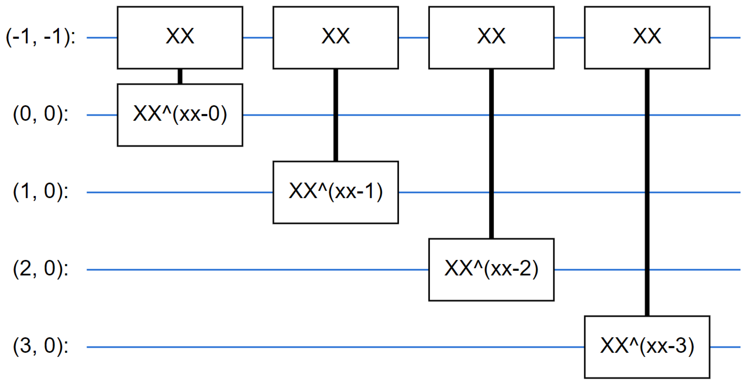
- The Quantum Neural Network, also known as QNN, was introduced in 2018 by Farhi et al. [38], and it represents a deep learning network exploiting only quantum operation (for this reason, we refer to the QNN also as a fully quantum model). Considering that the classification is based on the expectation of the readout qubit, the authors in [38] proposed the usage of two-qubit gates, with the readout qubit always acted upon. This is similar in some ways to running a small Unitary RNN across the pixels. The proposed QNN for malware detection exploits this approach, where each layer uses n instances of the same gate, with each of the data qubits acting on the readout qubit, by starting with a simple class that will add a layer of these gates to a circuit. Figure 5 shows an example of a circuit layer to better understand how it looks. The quantum circuit consists of a sequence of parameter-dependent unitary transformations, which act on an input quantum state. The input quantum state is an n-bit computational basis state corresponding to a sample string. The idea is to design a circuit made from two-qubit unitaries that can correctly represent the label of any Boolean function of n bits. Listing 3 shows the Python code related to the Quantum Neural Network we implemented. In particular, in Listing 3, two different layers are exploited: the first one is a Parametrized Quantum Circuit (PQC) layer, typically related to the fully quantum model, and the last one is a Dense layer used to perform the classification (as happens in a classic Convolutional Neural Network). The PQC level is considered for the training of parameterized quantum models. Given a parameterized circuit, this level initializes the parameters. We define a simple quantum circuit on a qubit. This circuit parameterizes an arbitrary rotation on the Bloch Sphere in terms of three angles, i.e., a, b, and c. The source code of the Quantum Neural Network developed by the authors is available, for research purposes, at the following link: https://github.com/vigimella/Quantum-Neural-Network (accessed on 26 October 2022).
model = models.Sequential ( )
model.add (layers.Conv2D (30 , (3, 3) , \
              activation =‘relu’,
              input_shape =(self.input_width_height,
			     self.input_width_height,
			     self.channels )))
model.add (layers.MaxPooling2D (pool_size =(2, 2)))
model.add (layers.Conv2D (15, (3, 3), \
              activation =‘relu’))
model.add (layers.MaxPooling2D (pool_size =(2, 2)))
model.add (layers.Dropout (0.25))
model.add (layers.Flatten ( ))
model.add (layers.Dense (128, activation =‘relu’))
model.add (layers.Dropout (0.5))
model.add (layers.Dense (50, activation =‘relu’))
model.add (layers.Dense (self.num_classes, \
              activation =‘softmax’))
NEW_SIZE = 10
[...]
model = models.Sequential ( )
model.add (QConv (filter_size =2, depth =8, \
   activation =‘relu’, name =‘qconv1’, \
   input_shape = (NEW_SIZE, NEW_SIZE, self.channels)))
model.add (layers.Conv2D (16 , (2, 2), \
   activation =‘relu’))
model.add (layers.Flatten ( ))
model.add (layers.Dense (32, activation =‘relu’))
model.add (layers.Dense (self.num_classes, \
   activation =‘softmax’))
[...]

model = models.Sequential ( )
model.add (PQC (model_circuit, model_readout))
model.add (layers.Dense (self.num_classes, activation =‘softmax’))
3.3. Experimental Analysis
3.4. Gradient-Weighted Class Activation Mapping
4. Results
5. Discussion
6. Related Work
7. Conclusions and Future Works
Author Contributions
Funding
Conflicts of Interest
References
- Mercaldo, F.; Santone, A. Deep learning for image-based mobile malware detection. J. Comput. Virol. Hacking Tech. 2020, 16, 157–171. [Google Scholar] [CrossRef]
- Casolare, R.; Lacava, G.; Martinelli, F.; Mercaldo, F.; Russodivito, M.; Santone, A. 2Faces: A new model of malware based on dynamic compiling and reflection. J. Comput. Virol. Hacking Tech. 2022, 18, 215–230. [Google Scholar] [CrossRef]
- Iadarola, G.; Martinelli, F.; Mercaldo, F.; Santone, A. Formal methods for android banking malware analysis and detection. In Proceedings of the 2019 IEEE Sixth International Conference on Internet of Things: Systems, Management and Security (IOTSMS), Granada, Spain, 22–25 October 2019; pp. 331–336. [Google Scholar]
- Kumar, K.A.; Raman, A.; Gupta, C.; Pillai, R. The Recent Trends in Malware Evolution, Detection and Analysis for Android Devices. J. Eng. Sci. Technol. Rev. 2020, 13, 240–248. [Google Scholar] [CrossRef]
- Cimitile, A.; Martinelli, F.; Mercaldo, F. Machine Learning Meets iOS Malware: Identifying Malicious Applications on Apple Environment. In Proceedings of the ICISSP, Porto, Portugal, 19–21 February 2017; pp. 487–492. [Google Scholar]
- Cimino, M.G.; De Francesco, N.; Mercaldo, F.; Santone, A.; Vaglini, G. Model checking for malicious family detection and phylogenetic analysis in mobile environment. Comput. Secur. 2020, 90, 101691. [Google Scholar] [CrossRef]
- Elsersy, W.F.; Feizollah, A.; Anuar, N.B. The rise of obfuscated Android malware and impacts on detection methods. Peerj Comput. Sci. 2022, 8, e907. [Google Scholar] [CrossRef] [PubMed]
- Dave, D.D.; Rathod, D. Systematic Review on Various Techniques of Android Malware Detection. In Proceedings of the International Conference on Computing Science, Communication and Security, Mehsana, India, 6–7 February 2022; pp. 82–99. [Google Scholar]
- Ferrante, A.; Medvet, E.; Mercaldo, F.; Milosevic, J.; Visaggio, C.A. Spotting the malicious moment: Characterizing malware behavior using dynamic features. In Proceedings of the IEEE 2016 11th International Conference on Availability, Reliability and Security (ARES), Salzburg, Austria, 31 August–2 September 2016; pp. 372–381. [Google Scholar]
- Casolare, R.; Ciaramella, G.; Iadarola, G.; Martinelli, F.; Mercaldo, F.; Santone, A.; Tommasone, M. On the Resilience of Shallow Machine Learning Classification in Image-based Malware Detection. Procedia Comput. Sci. 2022, 207, 145–157. [Google Scholar] [CrossRef]
- Yuxin, D.; Siyi, Z. Malware detection based on deep learning algorithm. Neural Comput. Appl. 2019, 31, 461–472. [Google Scholar] [CrossRef]
- Buduma, N.; Buduma, N.; Papa, J. Fundamentals of Deep Learning; O’Reilly Media, Inc.: Sevastopol, CA, USA, 2022. [Google Scholar]
- Giannotti, F. Explainable Machine Learning for trustworthy AI. In Artificial Intelligence Research and Development; IOS Press: Amsterdam, The Netherlands, 2022; p. 3. [Google Scholar]
- Pedreschi, D.; Giannotti, F.; Guidotti, R.; Monreale, A.; Ruggieri, S.; Turini, F. Meaningful explanations of black box AI decision systems. In Proceedings of the AAAI Conference on Artificial Intelligence, Honolulu, HI, USA, 27 January–1 February 2019; Volume 33, pp. 9780–9784. [Google Scholar]
- Schuld, M.; Sinayskiy, I.; Petruccione, F. An introduction to quantum Machine Learning. Contemp. Phys. 2015, 56, 172–185. [Google Scholar] [CrossRef]
- Martín-Guerrero, J.D.; Lamata, L. Quantum Machine Learning: A tutorial. Neurocomputing 2022, 470, 457–461. [Google Scholar] [CrossRef]
- Ciaramella, G.; Iadarola, G.; Mercaldo, F.; Storto, M.; Santone, A.; Martinelli, F. Introducing Quantum Computing in Mobile Malware Detection. In Proceedings of the 17th International Conference on Availability, Reliability and Security, Vienna, Austria, 23–26 August 2022; pp. 1–8. [Google Scholar]
- Gandotra, E.; Bansal, D.; Sofat, S. Malware analysis and classification: A survey. J. Inf. Secur. 2014, 2014, 44440. [Google Scholar] [CrossRef]
- Massoli, F.V.; Vadicamo, L.; Amato, G.; Falchi, F. A Leap among Entanglement and Neural Networks: A Quantum Survey. arXiv 2021, arXiv:2107.03313. [Google Scholar]
- Vasan, D.; Alazab, M.; Wassan, S.; Safaei, B.; Zheng, Q. Image-Based malware classification using ensemble of CNN architectures (IMCEC). Comput. Secur. 2020, 92, 101748. [Google Scholar] [CrossRef]
- Iadarola, G.; Martinelli, F.; Mercaldo, F.; Santone, A. Towards an interpretable deep learning model for mobile malware detection and family identification. Comput. Secur. 2021, 105, 102198. [Google Scholar] [CrossRef]
- Hirvensalo, M. Quantum Computing; Springer Science & Business Media: Berlin, Germany, 2003. [Google Scholar]
- Gill, S.S.; Kumar, A.; Singh, H.; Singh, M.; Kaur, K.; Usman, M.; Buyya, R. Quantum computing: A taxonomy, systematic review and future directions. Softw. Pract. Exp. 2022, 52, 66–114. [Google Scholar] [CrossRef]
- Boyer, M.; Liss, R.; Mor, T. Geometry of entanglement in the Bloch Sphere. Phys. Rev. A 2017, 95, 032308. [Google Scholar] [CrossRef]
- Rebentrost, P.; Mohseni, M.; Lloyd, S. Quantum support vector machine for big data classification. Phys. Rev. Lett. 2014, 113, 130503. [Google Scholar] [CrossRef]
- Wiebe, N.; Kapoor, A.; Svore, K.M. Quantum deep learning. arXiv 2014, arXiv:1412.3489. [Google Scholar] [CrossRef]
- Lloyd, S.; Mohseni, M.; Rebentrost, P. Quantum algorithms for supervised and unsupervised Machine Learning. arXiv 2013, arXiv:1307.0411. [Google Scholar]
- Shor, P.W. Polynomial-time algorithms for prime factorization and discrete logarithms on a quantum computer. SIAM Rev. 1999, 41, 303–332. [Google Scholar] [CrossRef]
- Aïmeur, E.; Brassard, G.; Gambs, S. Machine Learning in a quantum world. In Proceedings of the Conference of the Canadian Society for Computational Studies of Intelligence, Québec City, QC, Canada, 7–9 June 2006; pp. 431–442. [Google Scholar]
- LeCun, Y.; Bottou, L.; Bengio, Y.; Haffner, P. Gradient-based learning applied to document recognition. Proc. IEEE 1998, 86, 2278–2324. [Google Scholar] [CrossRef]
- Khan, S.; Rahmani, H.; Shah, S.A.A.; Bennamoun, M. A guide to Convolutional Neural Networks for computer vision. Synth. Lect. Comput. Vis. 2018, 8, 1–207. [Google Scholar]
- Krizhevsky, A.; Sutskever, I.; Hinton, G.E. Imagenet classification with deep Convolutional Neural Networks. Adv. Neural Inf. Process. Syst. 2012, 25, 1097–1105. [Google Scholar] [CrossRef]
- Simonyan, K.; Zisserman, A. Very deep convolutional networks for large-scale image recognition. arXiv 2014, arXiv:1409.1556. [Google Scholar]
- Selvaraju, R.R.; Cogswell, M.; Das, A.; Vedantam, R.; Parikh, D.; Batra, D. Grad-cam: Visual explanations from deep networks via gradient-based localization. In Proceedings of the IEEE International Conference on Computer Vision, Venice, Italy, 22–29 October 2017; pp. 618–626. [Google Scholar]
- Howard, A.G.; Zhu, M.; Chen, B.; Kalenichenko, D.; Wang, W.; Weyand, T.; Andreetto, M.; Adam, H. Mobilenets: Efficient Convolutional Neural Networks for mobile vision applications. arXiv 2017, arXiv:1704.04861. [Google Scholar]
- Tan, M.; Le, Q. Efficientnet: Rethinking model scaling for convolutional neural networks. In Proceedings of the International conference on Machine Learning. PMLR, Vancouver, BC, Canada, 13 December 2019; pp. 6105–6114. [Google Scholar]
- Broughton, M.; Verdon, G.; McCourt, T.; Martinez, A.J.; Yoo, J.H.; Isakov, S.V.; Massey, P.; Halavati, R.; Niu, M.Y.; Zlokapa, A.; et al. Tensorflow quantum: A software framework for quantum machine learning. arXiv 2020, arXiv:2003.02989. [Google Scholar]
- Farhi, E.; Neven, H. Classification with quantum neural networks on near term processors. arXiv 2018, arXiv:1802.06002. [Google Scholar]
- Zhou, B.; Khosla, A.; Lapedriza, A.; Oliva, A.; Torralba, A. Learning deep features for discriminative localization. In Proceedings of the IEEE Conference on Computer Vision and Pattern Recognition, Las Vegas, NV, USA, 27–30 June 2016; pp. 2921–2929. [Google Scholar]
- Bacci, A.; Bartoli, A.; Martinelli, F.; Medvet, E.; Mercaldo, F. Detection of obfuscation techniques in android applications. In Proceedings of the 13th International Conference on Availability, Reliability and Security, Hamburg, Germany, 27–30 August 2018; pp. 1–9. [Google Scholar]
- Bacci, A.; Bartoli, A.; Martinelli, F.; Medvet, E.; Mercaldo, F.; Visaggio, C.A. Impact of Code Obfuscation on Android Malware Detection based on Static and Dynamic Analysis. In Proceedings of the ICISSP, Funchal, Portugal, 22–24 January 2018; pp. 379–385. [Google Scholar]
- Amin, J.; Sharif, M.; Gul, N.; Kadry, S.; Chakraborty, C. Quantum Machine Learning architecture for COVID-19 classification based on synthetic data generation using conditional adversarial neural network. Cogn. Comput. 2022, 14, 1677–1688. [Google Scholar] [CrossRef] [PubMed]
- Seymour, J.J. Quantum Classification of Malware; University of Maryland, Baltimore County: Baltimore, MD, USA, 2014. [Google Scholar]
- Allgood, N.R. A Quantum Algorithm to Locate Unknown Hashes for Known n-Grams Within a Large Malware Corpus. Ph.D. Thesis, University of Maryland, Baltimore County, Baltimore, MD, USA, 2020. [Google Scholar]
- Rey, V.; Sánchez, P.M.S.; Celdrán, A.H.; Bovet, G. Federated learning for malware detection in iot devices. Comput. Netw. 2022, 204, 108693. [Google Scholar] [CrossRef]
- Yadav, P.; Menon, N.; Ravi, V.; Vishvanathan, S.; Pham, T.D. EfficientNet Convolutional Neural Networks-based Android malware detection. Comput. Secur. 2022, 115, 102622. [Google Scholar] [CrossRef]
- Venkatraman, S.; Alazab, M.; Vinayakumar, R. A hybrid deep learning image-based analysis for effective malware detection. J. Inf. Secur. Appl. 2019, 47, 377–389. [Google Scholar] [CrossRef]
- Pitolli, G.; Aniello, L.; Laurenza, G.; Querzoni, L.; Baldoni, R. Malware family identification with BIRCH clustering. In Proceedings of the 2017 International Carnahan Conference on Security Technology (ICCST), Madrid, Spain, 23–26 October 2017; pp. 1–6. [Google Scholar] [CrossRef]
- Kinable, J.; Kostakis, O. Malware classification based on call graph clustering. J. Comput. Virol. 2011, 7, 233–245. [Google Scholar] [CrossRef]
- Liangboonprakong, C.; Sornil, O. Classification of malware families based on N-grams sequential pattern features. In Proceedings of the 2013 IEEE 8th Conference on Industrial Electronics and Applications (ICIEA), Melbourne, VIC, Australia, 19–21 June 2013; pp. 777–782. [Google Scholar] [CrossRef]
- Boukhtouta, A.; Lakhdari, N.E.; Debbabi, M. Inferring Malware Family through Application Protocol Sequences Signature. In Proceedings of the 2014 6th International Conference on New Technologies, Mobility and Security (NTMS), Dubai, United Arab Emirates, 30 March–2 April 2014; pp. 1–5. [Google Scholar] [CrossRef]
- Zhong, Y.; Yamaki, H.; Yamaguchi, Y.; Takakura, H. Ariguma code analyzer: Efficient variant detection by identifying common instruction sequences in malware families. In Proceedings of the 2013 IEEE 37th Annual Computer Software and Applications Conference, Kyoto, Japan, 22–26 July 2013; pp. 11–20. [Google Scholar]
- Huang, K.; Ye, Y.; Jiang, Q. ISMCS: An intelligent instruction sequence based malware categorization system. In Proceedings of the 2009 3rd International Conference on Anti-counterfeiting, Security, and Identification in Communication, Hong Kong, China, 20–22 August 2009; pp. 509–512. [Google Scholar] [CrossRef]
- Martinelli, F.; Mercaldo, F.; Michailidou, C.; Saracino, A. Phylogenetic Analysis for Ransomware Detection and Classification into Families. In Proceedings of the SECRYPT, Porto, Portugal, 26–28 July 2018; pp. 732–737. [Google Scholar]


| Model | Image Size | Batch | Epochs | Learning Rate | Training Time (HH:MM:SS) |
|---|---|---|---|---|---|
| AlexNet | 110 × 1 | 32 | 50 | 0.001 | 0:47:14 |
| Standard-CNN | 110 × 1 | 32 | 50 | 0.001 | 1:11:54 |
| Standard-CNN | 25 × 3 | 64 | 20 | 0.001 | 0:01:34 |
| VGG16 | 110 × 3 | 32 | 25 | 0.001 | 2:56:45 |
| MobileNet | 110 × 3 | 64 | 25 | 0.001 | 0:22:45 |
| VGG19 | 110 × 3 | 64 | 25 | 0.001 | 3:35:56 |
| EfficientNet | 110 × 3 | 64 | 25 | 0.001 | 0:36:25 |
| EfficientNet | 25 × 3 | 64 | 20 | 0.001 | 0:07:26 |
| Hybrid-CNN | 25 × 1 | 32 | 20 | 0.010 | 1 day, 5:39:14 |
| QNN | 4 × 1 | 64 | 10 | 0.010 | 0:10:34 |
| Model | Loss | Accuracy | Precision | Recall | F-Measure | AUC |
|---|---|---|---|---|---|---|
| AlexNet | 0.435 | 0.912 | 0.920 | 0.908 | 0.914 | 0.983 |
| Standard-CNN (110 × 3) | 0.205 | 0.970 | 0.972 | 0.970 | 0.971 | 0.993 |
| Standard-CNN (25 × 3) | 0.260 | 0.915 | 0.927 | 0.910 | 0.919 | 0.993 |
| VGG16 | 0.182 | 0.952 | 0.959 | 0.949 | 0.954 | 0.993 |
| MobileNet | 0.124 | 0.966 | 0.969 | 0.963 | 0.966 | 0.996 |
| VGG19 | 0.187 | 0.951 | 0.953 | 0.947 | 0.950 | 0.994 |
| EfficientNet (110 × 3) | 23.738 | 0.065 | 0.065 | 0.065 | 0.065 | 0.455 |
| EfficientNet (25 × 3) | 2.343 | 0.251 | 0.135 | 0.022 | 0.038 | 0.535 |
| Hybrid-QCNN | 1.045 | 0.905 | 0.905 | 0.903 | 0.904 | 0.962 |
| QNN | 1.584 | 0.413 | 0.623 | 0.103 | 0.176 | 0.762 |
| Output Classes | Models | Accuracy | Precision | Recall | F-Measure | AUC |
|---|---|---|---|---|---|---|
| Airpush | Standard-CNN | 0.979 | 0.906 | 0.952 | 0.929 | 0.968 |
| Hybrid-QCNN | 0.951 | 0.837 | 0.811 | 0.824 | 0.893 | |
| Dowgin | Standard-CNN | 0.978 | 0.902 | 0.848 | 0.874 | 0.919 |
| Hybrid-QCNN | 0.945 | 0.694 | 0.703 | 0.699 | 0.836 | |
| FakeInst | Standard-CNN | 0.997 | 0.990 | 1.0 | 0.995 | 0.998 |
| Hybrid-QCNN | 0.991 | 0.985 | 0.978 | 0.982 | 0.987 | |
| Fusob | Standard-CNN | 0.999 | 0.996 | 1.0 | 0.998 | 0.999 |
| Hybrid-QCNN | 0.998 | 0.988 | 1.0 | 0.994 | 0.998 | |
| Jisut | Standard-CNN | 0.996 | 0.956 | 0.990 | 0.973 | 0.993 |
| Hybrid-QCNN | 0.994 | 0.971 | 0.936 | 0.953 | 0.967 | |
| Mecor | Standard-CNN | 0.999 | 1.0 | 0.996 | 0.998 | 0.998 |
| Hybrid-QCNN | 0.998 | 0.996 | 0.996 | 0.996 | 0.997 | |
| Trusted | Standard-CNN | 0.976 | 0.930 | 0.882 | 0.905 | 0.936 |
| Hybrid-QCNN | 0.930 | 0.714 | 0.745 | 0.729 | 0.851 |
Publisher’s Note: MDPI stays neutral with regard to jurisdictional claims in published maps and institutional affiliations. |
© 2022 by the authors. Licensee MDPI, Basel, Switzerland. This article is an open access article distributed under the terms and conditions of the Creative Commons Attribution (CC BY) license (https://creativecommons.org/licenses/by/4.0/).
Share and Cite
Mercaldo, F.; Ciaramella, G.; Iadarola, G.; Storto, M.; Martinelli, F.; Santone, A. Towards Explainable Quantum Machine Learning for Mobile Malware Detection and Classification. Appl. Sci. 2022, 12, 12025. https://doi.org/10.3390/app122312025
Mercaldo F, Ciaramella G, Iadarola G, Storto M, Martinelli F, Santone A. Towards Explainable Quantum Machine Learning for Mobile Malware Detection and Classification. Applied Sciences. 2022; 12(23):12025. https://doi.org/10.3390/app122312025
Chicago/Turabian StyleMercaldo, Francesco, Giovanni Ciaramella, Giacomo Iadarola, Marco Storto, Fabio Martinelli, and Antonella Santone. 2022. "Towards Explainable Quantum Machine Learning for Mobile Malware Detection and Classification" Applied Sciences 12, no. 23: 12025. https://doi.org/10.3390/app122312025
APA StyleMercaldo, F., Ciaramella, G., Iadarola, G., Storto, M., Martinelli, F., & Santone, A. (2022). Towards Explainable Quantum Machine Learning for Mobile Malware Detection and Classification. Applied Sciences, 12(23), 12025. https://doi.org/10.3390/app122312025