
Experimental Tests for Fluorescence LIDAR Remote Sensing of Submerged Plastic Marine Litter

“Nello Carrara” Institute of Applied Physics, National Research Council, I-50019 Sesto Fiorentino, Firenze, Italy
*
Author to whom correspondence should be addressed.
Remote Sens. 2022, 14(23), 5914; https://doi.org/10.3390/rs14235914
Submission received: 23 September 2022
/
Revised: 18 November 2022
/
Accepted: 19 November 2022
/
Published: 22 November 2022
(This article belongs to the Section Environmental Remote Sensing)
Abstract
:Marine plastic litter has become a global challenge, affecting all regions of the planet, with massive plastic input to the marine environment every year. Novel remote sensing methods can greatly contribute to face this complex issue with their ability to provide large-scale data. Here we present experimental tests exploring the potential of the hyperspectral fluorescence LIDAR technique for the detection and characterization of plastics when plunged into a layer of natural water. The experiments were carried out in the laboratory by using an in-house developed fluorescence hyperspectral LIDAR with 355 nm excitation from a distance of 11 m on weathered commercial plastic samples plunged into natural water. Results showed the capability of the technique to detect the fluorescence features of several types of plastics, also when plunged into water, and to decouple it from the fluorescence due to colored dissolved organic matter and from Raman scattering due to water molecules. Discrimination of plastics against other marine debris, e.g., vegetation and wood, has also been discussed. The study lays a basis for fluorescence LIDAR remote sensing of plastics in marine environment and paves the way to the detection of MPL also in conditions (e.g., submerged or transparent plastics) that are likely to be challenging by using other passive remote sensing techniques.

1. Introduction
Marine plastic litter (MPL) has become a global challenge, affecting all regions of the planet from the remote Antarctic and Arctic regions [1,2,3,4,5] to coastal areas and beaches of densely populated countries [6], yielding unprecedented impact on marine life, maritime industries, leisure activities and human health [7,8,9]. On the other hand, the investigation of the MPL issue has revealed itself to be increasingly complex and challenging. This is reflected also by a growing effort in the scientific community in terms of research and development studies, as testified by the large amount of papers published on this topic, reaching more than 3000 papers in the 2015–2020 period [10].
Plastics production has been growing incredibly fast, with an increase in the last years from 335 million tons in 2016 to 368 million tons in 2020. Only in 2021, there was a slight decrease due to the COVID-19 pandemic with a global production of 367 tons [11], with estimated input to the marine environment between 6 and 13 million tons every year [12,13]. Since it was found that there was a general discrepancy between the expected amount of plastics to have entered the marine environment and the actual estimate of MPL based on collected data, several works have suggested coastline and seafloor as possible sinks [14,15].
In general, MPL in the ocean can vary in type, shape, dimensions, chemical composition and buoyancy to a large extent [16,17,18]. Although most of it is originated from land, MPL is further fragmented by the action of the water and the waves, and it is dispersed by currents in the ocean to become a global issue. Quantifying MPL, understanding its main sources and identifying its major routes and accumulation sites are essential to implement future policies aimed at mitigating the MPL impact. Under this respect, remote sensing techniques could offer a unique opportunity to tackle the MPL issue on a large scale.
To date, a variety of remote sensing techniques have been studied for their application to MPL detection and characterization, yet with a different degree of maturity and success. Remote sensing techniques have already been applied in several experiments under controlled conditions and, in some cases, also deployed in real case scenarios (ocean, along coastline and beaches) from different platforms (satellite, airplane, drones). Among these, we can mention: hyperspectral remote sensing, with the detection of MPL in a real case scenario such as the Great Pacific Garbage Patch by using a hyperspectral short wavelength infrared (SWIR) imager from airplane [19], experiments to increase the discrimination capabilities of the hyperspectral data [20,21], pansharpening techniques applied to hyperspectral PRISMA data [22] and hyperspectral imagers deployed from UAV [23]; multispectral imaging from satellite, with several studies conducted also using Sentinel-2 and WorldView3 data [6,24,25,26]; thermal infrared (TIR) remote sensing, with experiments carried out by using a TIR camera showing promising results for the detection of floating plastics [27], bistatic RADAR from satellite [28], and very high spatial resolution (VHR) images from a variety of platforms, including drones [29,30,31]. Despite a considerable number of studies and experiments carried out using different types of passive remote sensing sensors, up to now, there has been a very limited effort to investigate the potential of light detection and ranging (LIDAR) techniques, although the latter have been suggested in several reviews as potentially interesting techniques for the remote sensing of MPL [18,32,33].
LIDAR techniques, initially developed for atmospheric studies, have been subsequently applied to the study of the aquatic environment [34]. They can provide a variety of information for the investigation of the marine environment, from the characterization of ocean optical properties to the detection of dissolved organic matter, phytoplankton, zooplankton, but also pollutants such as oils [35,36,37,38,39,40,41]. Although there are not yet spaceborne LIDAR systems specifically designed for marine applications, currently there are several space missions with onboard LIDAR sensors, mainly for atmospheric science applications [42,43]. There is also an ongoing effort in the scientific community towards studies for the development of novel spaceborne LIDAR missions specifically designed for oceanographic applications as well as to exploit available LIDAR datasets—acquired thanks to ongoing LIDAR missions—and adapt them for marine-related applications such as the detection of microparticles in the ocean [44,45,46,47]. With respect to passive sensors, LIDAR systems offer the advantage to overcome limitations set by solar illumination conditions and even at night. In principle, they can also provide a vertical profiling of the penetrated water volume with depth-resolved information about water column content [34]. On the other hand, spatial and temporal resolution of LIDAR data are usually poor with respect to those provided by passive sensors. For example, the Cloud-Aerosol Lidar with Orthogonal Polarization (CALIOP) sensor aboard the CALIPSO satellite, designed however for atmospheric science applications, guarantees a spatial footprint of about 100 m [42].
Despite a general interest to investigate the potential of LIDAR techniques for the MPL issue, there is a considerable lack of studies and experiments on the subject, except for very sporadic elastic backscatter LIDAR data from airplane [48] and experiments conducted for marine debris detection on beaches [49,50]. On the other hand, fluorescence-based LIDAR techniques have not been investigated at all, although they could be beneficial for spectral characterization of PML, which would be particularly useful to help in discriminating MPL from other types of marine debris. Since the 1970s, fluorescence-based techniques have been extensively investigated in the laboratory as a rapid, non-destructive method for characterization of commercial plastics [51]. Subsequently, Laser Induced Fluorescence (LIF) spectra and fluorescence time decay by using an excimer laser as excitation source were studied for the characterization of commercial plastics [52]. Piruska et al. studied the autofluorescence properties of plastic materials as potential substitutes for glass substrates used in microfluidic systems [53], while HDPE films were characterized by the rate coefficient of the fluorescence intensity decay in [54]. Fluorescence lifetime was also proposed as a powerful tool for the identification of polymers and their sorting for recycling purposes [55]. Spizzichino et al. instead used LIF spectroscopy and Principal Component Analysis (PCA) to investigate fast detection of plastic debris in a post-blast scene [56]. Recently, fluorescence lifetime imaging microscopy has been suggested as a powerful investigation tool for identification and characterization of plastics [57]. Nonetheless, until now, fluorescence LIDAR experiments on plastics in simulated MPL scenario conditions have not been conducted.
This study presents the first LIDAR experimental data—acquired under controlled conditions in the laboratory—aimed at demonstrating the feasibility of detecting and characterizing plastics floating on the surface as well as plastics plunged into the first layer of the water column by using the fluorescence LIDAR technique. The study shows the spectral fluorescence signatures of different types of weathered, commercially available plastics and how these signatures can be exploited for plastics detection and characterization—also when they are submerged in the water—by means of a fluorescence LIDAR system. In addition, the study discusses other affecting factors such as the presence of dissolved organic matter in the water and compares the fluorescence spectra of plastics with the fluorescence features of other types of marine litter that can be typically found in a real case scenario.
2. Materials and Methods
In this section, we first describe the samples used for the experiments; secondly, we report the main specifications of the instrumentation used and we illustrate the experimental set-up; finally, we describe the procedures used for data processing.
2.1. Materials
Figure 1 shows the samples selected for the fluorescence LIDAR measurements. All the samples selected for the experiment were parts of commercially available items. All the samples were taken from weathered items, used for several years (>2 years), except for the surgical mask that was not used. The list of the samples, together with a short description and the material they are made of (when the information was available), are reported in Table 1.
2.2. Instrumentation
The fluorescence LIDAR system used for the measurements is a recently upgraded prototype of an in-house developed hyperspectral and time-resolved fluorescence LIDAR imager. The instrument acquires fluorescence spectra with more than 900 spectral channels in the 350 nm to 830 nm spectral range, temporal resolution of 5 ns and a target scanning system developed for the acquisition of hyperspectral/time-resolved fluorescence images [58].
As an excitation source, the upgraded version of this LIDAR system uses a 3ω Q-switched Nd:YAG laser (Quantel Laser by Lumibird, Lannion, France; Ultra 50 model) with an output energy of 12 mJ@355 nm and adjustable pulse repetition rate up to 20 Hz. A beam expander provides an optimal beam divergence corresponding to the Instantaneous Field Of View (IFOV) of the collection optics. The collection optics is made up by a 1000 mm focal length f/4 Newtonian telescope (Sky-Watcher, SunOptical, Tapei City, Taiwan; Quattro 250P model). The telescope focusses the fluorescence signal from the target on a bundle of low fluorescence-grade fused silica optical fibers, in front of which a longpass optical filter @390 nm is placed to reject the backscattered laser radiation and to avoid spectral orders overlapping. The latter is coupled to the input slit of a spectrometer (PI-Acton, Teledyne Princeton Instruments, Trenton, NJ, USA; SpectraPro 2300i model). The IFOV of the LIDAR is 1 mrad. The spectrometer (300 mm focal length, f/3.9) is equipped with three selectable different diffraction gratings (150 gg/mm, 600 gg/mm, 2400 gg/mm). The nominal spectral resolution of the system with the three gratings are 0.5 nm, 0.1 nm and 0.02 nm, respectively. The spectrometer is coupled to an intensified gated 512-pixel x 512-pixel CCD camera (PI-Acton, Teledyne Princeton Instruments, Trenton, NJ, USA; PI-Max:512 model). The triggering of the CCD gate allows to set an accurate delay from the laser pulse generation thus allowing the temporal resolution among different laser pulses. The pointing and scanning system of the LIDAR is implemented by means of a motorized altazimuth mount allowing a pointing accuracy of 25 µrad (Sky-Watcher, SunOptical, Tapei City, Taiwan; AZ-EQ6 model). The main technical specifications of the fluorescence LIDAR system are reported in Table 2.
2.3. Experimental Set-Up
The experimental set-up used for the fluorescence LIDAR measurements in the laboratory is shown in Figure 2.
All the measurements were carried out in the laboratory under ambient light conditions. The fluorescence LIDAR system was placed at a distance from the samples of about 11 m. At this distance, the area on the target that is seen by the LIDAR is a 1 cm diameter spot. This distance guarantees to avoid meaningful obscuration form the secondary mirror of the telescope.
In order to carry out measurements on samples immersed into the water, we used a cylindrical container that allows to simulate the effect of a water column above the sample up to a height of about 50 cm. The cylindrical container has an internal diameter of 35 cm and its height is about 60 cm (Figure 2b). The bottom of the container is covered with a black foil of material with a very low fluorescence efficiency. This setup was adopted in order to reproduce realistic experimental conditions at sea in which the laser beam is attenuated by the water column and the main contributions to the fluorescence signal are due to the water column content, such as Colored Dissolved Organic Matter (CDOM) and phytoplankton, rather than to the sea floor.
A 45° folding mirror (Figure 2b) was placed on the opened top end of the container in order to deflect the laser beam coming from the LIDAR vertically inside the container. The width/height ratio of the container is lower than that between the diameter of the LIDAR collection optics and the working distance: in the central part of the container diameter, and all through its height, it is therefore possible to acquire the fluorescence signal without vignetting from the walls of the container.
Two series of measurements were carried out: the first series (dry samples) was carried out on the samples placed at the bottom of the empty container. The second series (wet samples) was carried out on the samples by placing them on the bottom of the container filled with tap water up to a height of 50 cm (Figure 2b). All the samples were measured in both conditions, except for sample M (polystyrene) which was measured only in dry conditions.
2.4. Data Acquisition Procedure
In order to obtain a fluorescence spectrum in the 350–810 nm spectral range with a nominal spectral sampling of 0.51 nm, two different—partially overlapped—measurements are acquired in the 350–610 nm and 550–810 nm spectral ranges, respectively. Each of these fluorescence spectra is the result of the subtraction between one (active) spectrum acquired while the laser is on and one (background) spectrum acquired while the laser is off with the same parameter settings. Typically, several couples of active/background measurements are acquired over several laser shots in order to average the results and to increase the signal-to-noise ratio. During the experiment, all fluorescence spectra were averaged over 10 laser shots with a pulse repetition rate of 20 Hz. The uncertainties σ associated to the measured fluorescence spectra are given by:
where S is the signal intensity and N is the number of laser shots (equal to 10, in this experiment). All measurements were corrected for the instrument’s spectral response function.
3. Results
In this section, we first describe the hyperspectral fluorescence LIDAR spectra obtained on different types of commercial plastics. Secondly, we show the fluorescence LIDAR spectra obtained on the samples when the latter are immersed into the water and compare them with the fluorescence spectra typical of natural waters, which include a fluorescence contribution due to CDOM. Finally, we show the spectra of other typical marine debris that can be found in a real scenario and compare their fluorescence properties with those of the studied plastics samples to assess to which extent they can affect the detection of plastics.
3.1. Fluorescence LIDAR Measurements of Different Types of Plastics
The first series (dry samples) of fluorescence LIDAR measurements was carried out on the dry samples of commercial plastics in order to investigate their fluorescence spectral features.
Figure 3 shows the fluorescence spectra of the dry samples: the spectra were acquired with excitation wavelength at 355 nm, from a distance of 11 m and in ambient light. Each fluorescence spectrum was obtained as an average over 10 laser shots. Figure 3a,b show the fluorescence spectra of samples in relative units, including the fluorescence spectrum of the black foil (Black F) used as a background at the bottom of the container and whose fluorescence emission is negligible with respect to the one of the examined samples. Figure 3c,d show the fluorescence spectra of the same samples, normalized to their standard deviation in order to make easier the comparison of their spectral shapes. All samples showed a detectable fluorescence emission with a maximum between 410 nm and 450 nm, except for sample G (HDPE, blue bottle cap) that had a fluorescence maximum emission at longer wavelength (470 nm, approximately) and sample J (latex, surgical glove) that had a maximum at 395 nm. All PET samples (A, B, H, I, L samples) featured a very intense fluorescence band with a maximum at 410–420 nm (Figure 3a). Only sample B (blue-colored PET bottle) had a slightly less intense fluorescence spectrum (Figure 3a), although its spectral shape is definitely similar to that of all other PET samples (Figure 3c). In Figure 3c, it can be also noted that the fluorescence spectrum of the white PET bottle (sample H) has its maximum at 420 nm, slightly shifted with respect to the one of the other PET samples. In addition to the PET samples, PVC blister (sample D) and the latex glove (sample J) also showed an intense fluorescence characterized by a peculiar spectral shape due to several fluorescence contributions (red and light green lines in Figure 3a). HDPE bottle caps, the chirurgical mask and the white plastic bag sample (samples F, G, C and E in Figure 3b, respectively) are fluorescent, yet definitely to a lesser extent. It is to be noted that all samples containing PET plastics (A, B, H, I, L samples) have an intense, relatively narrow fluorescence band centered at about 410–420 nm and 50 nm wide; all the other commercial samples show fluorescence spectra with several contributions between 400 nm and 600 nm. Among the less fluorescent samples (Figure 3d), the used white plastic bag (unknown material) showed a spectral shape very similar to that of sample K (transparent packaging in polypropylene) and of the low-fluorescent black foil used as a background (black alveolar sheet in polypropylene). Fluorescence intensity is of course affected by additives and dyes mixed with the polymer, yet the main features of the spectral shape remain unchanged.
3.2. Fluorescence LIDAR Measurements of Submerged Plastics
The second series (wet samples) of fluorescence LIDAR measurements was carried out on the samples submerged into a water column of 50 cm. All the spectra were acquired with excitation wavelength at 355 nm, from a distance of 11 m and in ambient light. Each fluorescence spectrum was obtained as an average over 10 laser shots.
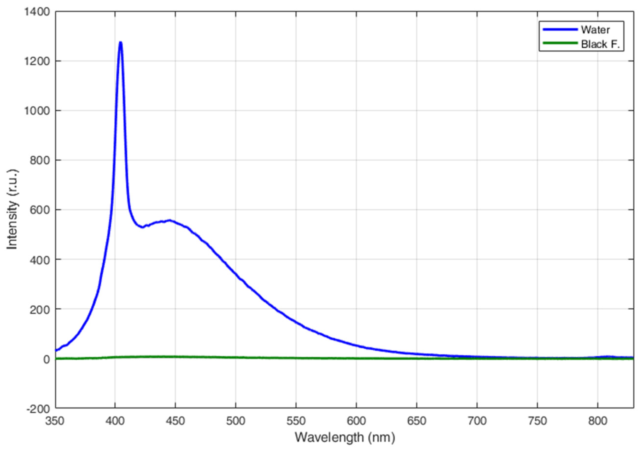
Figure 4 shows the fluorescence LIDAR spectrum obtained on the water column of the container with the only black low-fluorescent sheet on the bottom. In the same graph, we also reported the fluorescence LIDAR spectrum of the black sheet (background) placed at the bottom of the container, whose fluorescence contribution is, in fact, negligible (green line in Figure 4). The spectrum of the water clearly shows a considerable fluorescence contribution due to CDOM with a maximum at about 440 nm. Moreover, the spectrum shows the typical Raman scattering signal at 404 nm due to the OH-stretching of the water molecules. This is the typical fluorescence LIDAR spectrum that can be expected by measurements acquired in coastal waters with a significant CDOM fluorescence contribution [59].
Figure 5 shows all the fluorescence LIDAR spectra acquired on the different samples of plastics (sample A through L) when these were plunged into the 50 cm water column. For the sake of clarity, the fluorescence LIDAR spectrum of the correspondent water column (without plastics) is also reported in Figure 5 (cyan dashed line). All spectra had the contribution due to the water Raman signal centered at 404 nm, although the latter is definitely less apparent in the spectra obtained on the strongly fluorescent PET samples. In general, all strongly fluorescent plastic samples (samples A, B, D, H, I, J, L) showed a fluorescence contribution that can be easily detected as a major, abrupt change in the fluorescence intensity of the spectrum, especially in the 410–470 nm spectral range. On the other hand, the less fluorescent samples (samples C, E, F, G, K) show a fluorescence contribution of plastics that can be hardly decoupled from that due to the CDOM present in the water column.
In order to remove the contributions of Raman scattering and of CDOM fluorescence from the spectra of plastic samples in Figure 5, we subtracted the acquired LIDAR spectrum obtained on the water column with the only black low-fluorescent sheet on the bottom (blue line in Figure 4). A first estimate σtot of the uncertainties on the measurement of strongly fluorescent plastics such as PET follows error propagation rules for the subtraction of two signals and it is proportional to:
where Sp and Sw are the two averaged fluorescence signals referring to the plastic and the sea water, respectively, and N is the number of laser shots.
The procedure has been applied to all spectra acquired on the plastic samples submerged into the water column (Figure 5). The results are reported in Figure 6, which shows the corrected fluorescence spectrum of each plastic sample retrieved from the fluorescence spectrum measured when the sample was plunged into the water. For comparison, the retrieved fluorescence spectrum of each sample is reported together with the fluorescence spectrum of the corresponding dry sample. In general, there is a very good agreement between the retrieved spectrum and the corresponding spectrum acquired on the dry sample for all the samples exhibiting medium to high fluorescence efficiency. The procedure still provides an acceptable corrected spectrum also for those samples with low fluorescence emission (samples C, E, G, K), although in this case, the retrieved spectra are very noisy. The intensity of all corrected spectra, however, is decreased, mainly due to the effects of the water layer.
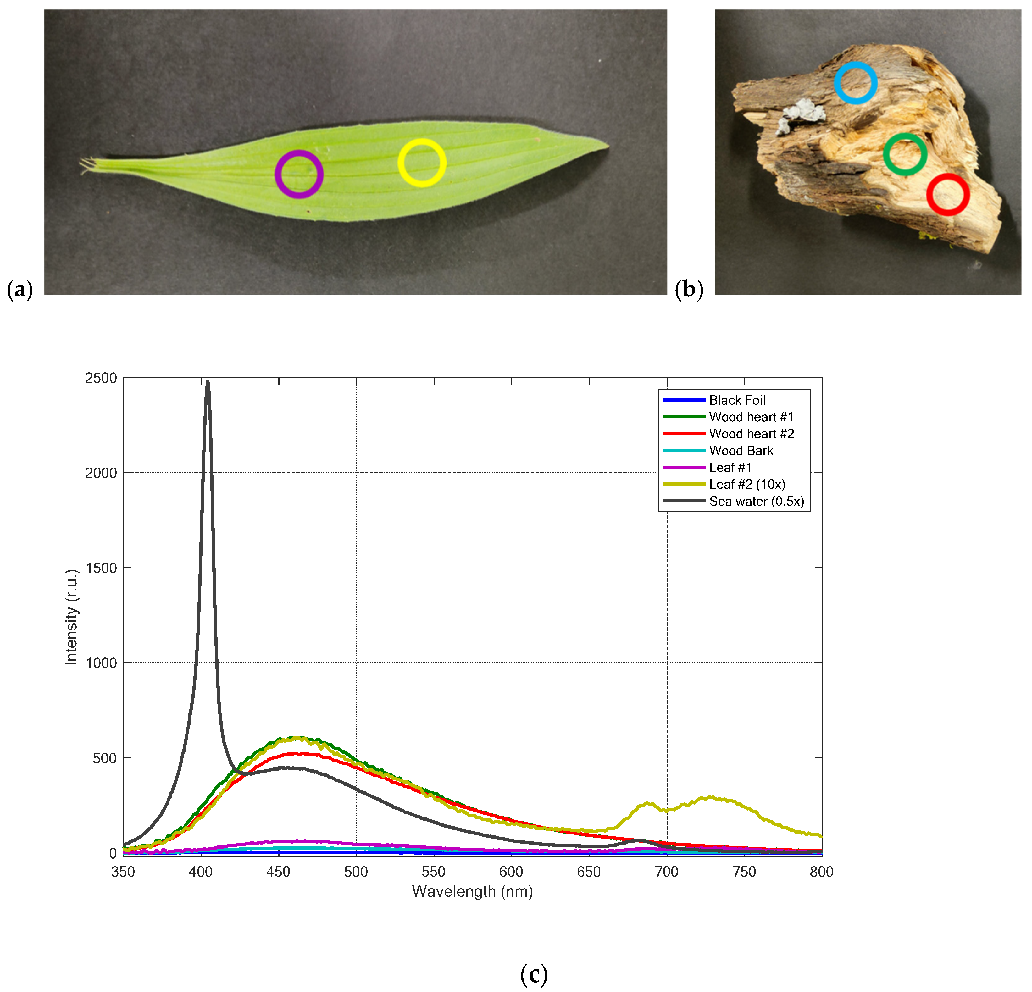
In order to investigate the feasibility of distinguishing plastics from other typical marine debris featuring fluorescence properties, we acquired fluorescence spectra also on wood logs and vegetation. The latter, in fact, can be typically found in a marine scenario and can contribute, in addition to CDOM, to the fluorescence spectrum collected in natural waters. Figure 7 shows the fluorescence spectra acquired in different spots of a wooden log, including the bark, and on two spots of a leaf. For a clearer visualization, the spectrum acquired on leaf spot #2 was multiplied by a factor of 10. In the same graph, for the sake of comparison, we also reported the fluorescence of the black foil used as a background and the typical fluorescence spectrum obtained in sea water featuring the Raman signal and the fluorescence contribution due to phytoplankton.
The fluorescence spectra, detected on a log of wood (Quercus L.), were acquired on both the wood heart and the wood bark. All the fluorescence spectra showed a maximum at about 460 nm, which is consistent with the fluorescence features of wood typically due to the presence of lignin when excited at 355 nm [60].
The fluorescence spectra acquired on the leaf showed the typical fluorescence emission of vegetation in the red region of the spectrum, which is due to the presence of chlorophyll a, common to all plants. It is characterized by two fluorescence bands at about 680 nm and 740 nm that are tightly linked to photosystems II and I [61,62]. The typical fluorescence peak of chlorophyll at about 680 nm is also widely used for the detection of phytoplankton—including macroalgae that can represent another type of marine debris—in natural waters [63].
4. Discussion
The experimental results presented here are the first fluorescence hyperspectral data acquired by using a fluorescence LIDAR, in standoff configuration, on plastics samples plunged into a layer of natural water. The results clearly show how the fluorescence LIDAR technique—using an excitation wavelength at 355 nm—is able to detect the fluorescence signal of several types of weathered commercial plastic samples when the latter are suspended in a layer of natural water, and not necessarily floating on the surface. This stands also in the presence of a considerable fluorescence contribution of the CDOM in the water, as it is expected in a real case scenario, especially in coastal waters, and the Raman scattering signal due to the OH-stretching of the water molecules.
Among the examined commercial samples, the ones with the most intense fluorescence signal were the PET-containing plastic samples, which makes them an easily detectable target for a real case scenario. On the other hand, some plastic samples (HDPE- and PP-containing samples) showed only a faint fluorescence when excited at 355 nm, which can make it difficult to decouple it from the CDOM fluorescence in a real case scenario, depending on the class of waters and the corresponding CDOM content. It is interesting to note that the detection feasibility applies also to samples that, being transparent, cannot be detected easily by using, for example, VHR RGB cameras, especially if they are not floating on the surface. In particular, PET-containing samples, when excited at 355 nm, showed a very intense fluorescence signal with a relatively narrow (50 nm, approximately) Full-Width Half Maximum—(FWHM), which makes it easier for detection with respect to background fluorescence of the water column due to the CDOM, the latter being characterized by a wider emission contribution with FWHM of about 150 nm.
Fluorescence contributions from different types of marine debris, such as phytoplankton or vegetation, can be easily identified by means of hyperspectral fluorescence LIDAR thanks to their typical, well-known fluorescence band due to chlorophyll in the red region of the spectrum (Figure 7). This can be exploited as a signature to identify natural marine debris such as floating leaves, benthos or buoyant macroalgae, against plastic litter. On the other hand, wooden debris is expected to contribute to the fluorescence signal only to a minor extent, with a wider band (150 nm FWHM) and with a maximum extent at longer wavelengths (around 460 nm) with respect to PET-containing plastics. With reference to less fluorescent plastic types, the only sample that showed a fluorescence contribution with a maximum at about 460 nm was the blue-colored HDPE (sample G), although with a narrower band (100 nm FWHM).
A strategy to detect MPL from the fluorescence LIDAR spectra acquired in a real case scenario could consist of two steps. The first step will select the spectra—out of a time series—with an abrupt depression of the Raman signal with respect to the adjacent measurements: this step aims at selecting all the spectra that contains anthropogenic or natural litter floating on the sea surface or below it. The second step should rely on the retrieval of the spectral shape by means of the comparison with the spectral shape of the adjacent fluorescence measurements, the latter assumed to refer to the only water column content (including CDOM and phytoplankton).
The spectral shape of the examined weathered plastic samples, and those retrieved from the relevant fluorescence spectra when the samples are plunged into the water, are consistent with the fluorescence spectra found in the literature for commercial plastics obtained in the laboratory under UV illumination: in particular, the fluorescence band at about 410–420 nm, which is very intense in PET samples, can be attributed to the polymers [51] and it is consistent with fluorescence spectra recently acquired with 350 nm excitation on label-free PET nanoplastics [64]. The less intense band at about 440 nm present in the fluorescence spectrum of HDPE-containing samples can be attributed to a charge-transfer complex of HDPE with oxygen, as reported in [54].
It should be noted, however, that most studies related to autofluorescence and, more specifically, to LIF of plastics have addressed excitation sources emitting at shorter wavelengths, typically in the range between 245 nm (KrF excimer laser) and 337 nm (nitrogen ion laser). The choice of a shorter wavelengths (e.g., 266 nm as in [56]), actually allows for the detection of important fluorescence contributions at about 350 nm from carbonyl groups present in polymers based on chains of methylene groups, such as polyethylene and polypropylene, which can be useful for a thorough characterization of the type of plastics [56]. In this study, however, we focused our research on the 355 nm excitation provided by a tripled frequency Nd:YAG laser since the latter can be regarded as the most widely used in fluorescence LIDAR remote sensing applications to the marine environment: differently from 266 nm excitation, 355 nm wavelength can still provide a reasonably good penetration into the water column. On the other hand, longer wavelengths which could guarantee better penetration depth into the water column (blue-green-emitting lasers) would not be suitable to excite fluorescence of most of the examined samples since fluorescence maximum is expected between 400 nm and 500 nm. In general, solid-state laser sources offer a high reliability and ruggedness, which make them very suitable for field operation in the marine environment [46]. These are, in fact, the same class of lasers that have already been deployed also from spaceborne platforms—although for different application scenarios—and that can provide a sound basis for a future pathway towards fluorescence LIDAR missions from space dedicated to the marine scenarios [46].
Future research directions will extend the database of fluorescence signatures of raw and weathered plastics, including ocean- and beach-harvested plastics, and the execution of LIDAR measurements at sea, in a real case scenario.
5. Conclusions
This study has investigated the potential of the fluorescence LIDAR technique for the remote sensing of plastics submerged in natural water in order to address it as a tool for the remote sensing of plastics in marine scenarios. The results of the experiments, conducted in controlled conditions in the laboratory on different types of weathered commercial plastics from a distance of 11 m, showed the capability of the fluorescence LIDAR to detect the signatures of plastics also when submerged in natural water and to decouple them from the fluorescence due to CDOM and from Raman scattering due to the OH-stretching of the water molecules. Further fluorescence-affecting factors, such as phytoplankton suspended in the water column and other types of possible natural marine debris have also been discussed. The outcome of the study lays a basis for the remote sensing of plastics in the marine environment by means of the hyperspectral fluorescence LIDAR technique and paves the way to the detection and discrimination of MPL also in experimental conditions that are likely to be challenging by using other passive remote sensing techniques, such as plastics suspended below the water surface or transparent plastics. Future work will focus on ocean- and beach-harvested plastics, compared to raw plastics, and realistic marine scenarios.
Author Contributions
Conceptualization, V.R.; methodology, L.P. and V.R.; validation, L.P. and V.R.; formal analysis, L.P. and V.R.; investigation, L.P. and V.R.; resources, V.R.; Software and figure preparation, L.P.; data curation, L.P. and V.R.; writing, V.R.; supervision, V.R.; funding acquisition, V.R. All authors have read and agreed to the published version of the manuscript.
Funding
This research was partly funded by the Discovery Element of the European Space Agency’s Basic Activities, grant number 4000132184/20/NL/GLC. The view expressed in this publication can in no way be taken to reflect the official opinion of the European Space Agency.
Data Availability Statement
All data are available upon request by mail to the authors.
Acknowledgments
The authors would like to thank Andrea Donati for technical support regarding the experiments.
Conflicts of Interest
The authors declare no conflict of interest.
References
- Halsband, C.; Herzke, D. Plastic Litter in the European Arctic: What Do We Know? Emerg. Contam. 2019, 5, 308–318. [Google Scholar] [CrossRef]
- Strand, K.O.; Huserbråten, M.; Dagestad, K.-F.; Mauritzen, C.; Grøsvik, B.E.; Nogueira, L.A.; Melsom, A.; Röhrs, J. Potential Sources of Marine Plastic from Survey Beaches in the Arctic and Northeast Atlantic. Sci. Total Environ. 2021, 790, 148009. [Google Scholar] [CrossRef] [PubMed]
- Mallory, M.L.; Baak, J.; Gjerdrum, C.; Mallory, O.E.; Manley, B.; Swan, C.; Provencher, J.F. Anthropogenic Litter in Marine Waters and Coastlines of Arctic Canada and West Greenland. Sci. Total Environ. 2021, 783, 146971. [Google Scholar] [CrossRef] [PubMed]
- Barnes, D.K.A.; Walters, A.; Gonçalves, L. Macroplastics at Sea around Antarctica. Mar. Environ. Res. 2010, 70, 250–252. [Google Scholar] [CrossRef] [PubMed]
- Waller, C.L.; Griffiths, H.J.; Waluda, C.M.; Thorpe, S.E.; Loaiza, I.; Moreno, B.; Pacherres, C.O.; Hughes, K.A. Microplastics in the Antarctic Marine System: An Emerging Area of Research. Sci. Total Environ. 2017, 598, 220–227. [Google Scholar] [CrossRef] [Green Version]
- Ciappa, A.C. Marine Plastic Litter Detection Offshore Hawai’i by Sentinel-2. Mar. Pollut. Bull. 2021, 168, 112457. [Google Scholar] [CrossRef]
- MacLeod, M.; Arp, H.P.H.; Tekman, M.B.; Jahnke, A. The global threat from plastic pollution. Science 2021, 373, 61–65. [Google Scholar] [CrossRef]
- World Health Organization. Microplastics in Drinking-Water; World Health Organization: Geneva, Switzterland, 2019; ISBN 978-92-4-151619-8. [Google Scholar]
- Werner, S.; Budziak, A.; van Franeker, J.; Galgani, F.; Hanke, G.; Maes, T.; Matiddi, M.; Nilsson, P.; Oosterbaan, L.; Priestland, E.; et al. Harm caused by Marine Litter. In MSFD GES TG Marine Litter-Thematic Report; JRC Technical Report; EUR 28317 EN; Publication office of the European Union: Luxenbourg, 2016. [Google Scholar] [CrossRef]
- Haarr, M.L.; Falk-Andersson, J.; Fabres, J. Global Marine Litter Research 2015–2020: Geographical and Methodological Trends. Sci. Total Environ. 2022, 820, 153162. [Google Scholar] [CrossRef]
- PlasticsEurope: Plastics-the Facts 2021: An Analysis of European Plastics Production, Demand and Waste Data. Available online: https://plasticseurope.org/wp-content/uploads/2021/12/Plastics-the-Facts-2021-web-final.pdf (accessed on 4 August 2022).
- Lyons, B.P.; Cowie, W.J.; Maes, T.; Le Quesne, W.J.F. Marine Plastic Litter in the ROPME Sea Area: Current Knowledge and Recommendations. Ecotoxicol. Environ. Saf. 2020, 187, 109839. [Google Scholar] [CrossRef]
- Sabatira, F. Southeast Asia regional cooperation on tackling marine plastic litter. Lampung J. Int. Law 2020, 2, 69–84. [Google Scholar] [CrossRef]
- Lebreton, L.; Egger, M.; Slat, B. A Global Mass Budget for Positively Buoyant Macroplastic Debris in the Ocean. Sci. Rep. 2019, 9, 12922. [Google Scholar] [CrossRef] [Green Version]
- Olivelli, A.; Hardesty, B.D.; Wilcox, C. Coastal Margins and Backshores Represent a Major Sink for Marine Debris: Insights from a Continental-Scale Analysis. Environ. Res. Lett. 2020, 15, 074037. [Google Scholar] [CrossRef]
- Napper, I.E.; Thompson, R.C. Chapter 22-Marine Plastic Pollution: Other Than Microplastic. In Waste, 2nd ed.; Letcher, T.M., Vallero, D.A., Eds.; Academic Press: Cambridge, MA, USA, 2019; pp. 425–442. ISBN 978-0-12-815060-3. [Google Scholar]
- Maximenko, N.; Arvesen, J.; Asner, G.; Carlton, J.; Castrence, M.; Centurioni, L.; Chao, Y.; Chapman, J.; Chirayath, V.; Corradi, P.; et al. Remote Sensing of Marine Debris to Study Dynamics, Balances and Trends. 2017. Available online: https://ecocast.arc.nasa.gov/las/Reports%20and%20Papers/Marine-Debris-Workshop-2017.pdf (accessed on 5 August 2022).
- Martínez-Vicente, V.; Clark, J.R.; Corradi, P.; Aliani, S.; Arias, M.; Bochow, M.; Bonnery, G.; Cole, M.; Cózar, A.; Donnelly, R.; et al. Measuring Marine Plastic Debris from Space: Initial Assessment of Observation Requirements. Remote Sens. 2019, 11, 2443. [Google Scholar] [CrossRef] [Green Version]
- Garaba, S.P.; Aitken, J.; Slat, B.; Dierssen, H.M.; Lebreton, L.; Zielinski, O.; Reisser, J. Sensing Ocean Plastics with an Airborne Hyperspectral Shortwave Infrared Imager. Environ. Sci. Technol. 2018, 52, 11699–11707. [Google Scholar] [CrossRef]
- Tasseron, P.; van Emmerik, T.; Peller, J.; Schreyers, L.; Biermann, L. Advancing Floating Macroplastic Detection from Space Using Experimental Hyperspectral Imagery. Remote Sens. 2021, 13, 2335. [Google Scholar] [CrossRef]
- Goddijn-Murphy, L.; Peters, S.; van Sebille, E.; James, N.A.; Gibb, S. Concept for a Hyperspectral Remote Sensing Algorithm for Floating Marine Macro Plastics. Mar. Pollut. Bull. 2018, 126, 255–262. [Google Scholar] [CrossRef] [Green Version]
- Kremezi, M.; Kristollari, V.; Karathanassi, V.; Topouzelis, K.; Kolokoussis, P.; Taggio, N.; Aiello, A.; Ceriola, G.; Barbone, E.; Corradi, P. Pansharpening PRISMA Data for Marine Plastic Litter Detection Using Plastic Indexes. IEEE Access 2021, 9, 61955–61971. [Google Scholar] [CrossRef]
- Balsi, M.; Moroni, M.; Chiarabini, V.; Tanda, G. High-Resolution Aerial Detection of Marine Plastic Litter by Hyperspectral Sensing. Remote Sens. 2021, 13, 1557. [Google Scholar] [CrossRef]
- Biermann, L.; Clewley, D.; Martinez-Vicente, V.; Topouzelis, K. Finding Plastic Patches in Coastal Waters Using Optical Satellite Data. Sci. Rep. 2020, 10, 5364. [Google Scholar] [CrossRef]
- Themistocleous, K.; Papoutsa, C.; Michaelides, S.; Hadjimitsis, D. Investigating Detection of Floating Plastic Litter from Space Using Sentinel-2 Imagery. Remote Sens. 2020, 12, 2648. [Google Scholar] [CrossRef]
- Park, Y.-J.; Garaba, S.; Sainte-Rose, B. Detecting Great Pacific Garbage Patch Floating Plastic Litter Using WorldView-3 Satellite Imagery. Opt. Express 2021, 29, 35288. [Google Scholar] [CrossRef] [PubMed]
- Goddijn-Murphy, L.; Williamson, B. On Thermal Infrared Remote Sensing of Plastic Pollution in Natural Waters. Remote Sens. 2019, 11, 2159. [Google Scholar] [CrossRef] [Green Version]
- Evans, M.; Ruf, C. Toward the Detection and Imaging of Ocean Microplastics With a Spaceborne Radar. IEEE Trans. Geosci. Remote Sens. 2021, 60, 1–9. [Google Scholar] [CrossRef]
- Geraeds, M.; van Emmerik, T.; de Vries, R.; bin Ab Razak, M.S. Riverine Plastic Litter Monitoring Using Unmanned Aerial Vehicles (UAVs). Remote Sens. 2019, 11, 2045. [Google Scholar] [CrossRef] [Green Version]
- Gil, G.; Andriolo, U.; Gonçalves, L.; Sobral, P.; Bessa, F. Quantifying Marine Macro Litter Abundance on a Sandy Beach Using Unmanned Aerial Systems and Object-Oriented Machine Learning Methods. Remote Sens. 2020, 12, 2599. [Google Scholar] [CrossRef]
- Andriolo, U.; Gonçalves, G.; Bessa, F.; Sobral, P. Mapping Marine Litter on Coastal Dunes with Unmanned Aerial Systems: A Showcase on the Atlantic Coast. Sci. Total Environ. 2020, 736, 139632. [Google Scholar] [CrossRef]
- Mace, T.H. At-sea detection of marine debris: Overview of technologies, processes, issues, and options. Mar. Pollut. Bull. 2012, 65, 23–27. [Google Scholar] [CrossRef]
- Maximenko, N.; Corradi, P.; Law, K.L.; Van Sebille, E.; Garaba, S.P.; Lampitt, R.S.; Galgani, F.; Martinez-Vicente, V.; Goddijn-Murphy, L.; Veiga, J.M.; et al. Toward the Integrated Marine Debris Observing System. Front. Mar. Sci. 2019, 447. [Google Scholar] [CrossRef] [Green Version]
- Measures, R.M. Laser Remote Sensing: Fundamentals and Applications; Wiley-Interscience: New York, NY, USA, 1984. [Google Scholar]
- Rogers, S.R.; Webster, T.; Livingstone, W.; O’Driscoll, N.J. Airborne Laser-Induced Fluorescence (LIF) Light Detection and Ranging (LiDAR) for the Quantification of Dissolved Organic Matter Concentration in Natural Waters. Estuaries Coasts 2012, 35, 959–975. [Google Scholar] [CrossRef]
- Palmer, S.C.J.; Pelevin, V.V.; Goncharenko, I.; Kovács, A.W.; Zlinszky, A.; Présing, M.; Horváth, H.; Nicolás-Perea, V.; Balzter, H.; Tóth, V.R. Ultraviolet Fluorescence LiDAR (UFL) as a Measurement Tool for Water Quality Parameters in Turbid Lake Conditions. Remote Sens. 2013, 5, 4405–4422. [Google Scholar] [CrossRef]
- Churnside, J.H.; Brown, E.D.; Parker-Stetter, S.; Horne, J.K.; Hunt, G.L., Jr.; Hillgruber, N.; Sigler, M.F.; Vollenweider, J.J. Airborne Remote Sensing of a Biological Hot Spot in the Southeastern Bering Sea. Remote Sens. 2011, 3, 621–637. [Google Scholar] [CrossRef] [Green Version]
- Saito, Y.; Takano, K.; Kobayashi, F.; Kobayashi, K.; Park, H.-D. Development of a UV Laser-Induced Fluorescence Lidar for Monitoring Blue-Green Algae in Lake Suwa. Appl. Opt. 2014, 53, 7030–7036. [Google Scholar] [CrossRef] [PubMed]
- Liu, H.; Chen, P.; Mao, Z.; Pan, D.; He, Y. Subsurface Plankton Layers Observed from Airborne Lidar in Sanya Bay, South China Sea. Opt. Express 2018, 26, 29134–29147. [Google Scholar] [CrossRef]
- Churnside, J.H.; Thorne, R.E. Comparison of Airborne Lidar Measurements with 420 KHz Echo-Sounder Measurements of Zooplankton. Appl. Opt. 2005, 44, 5504–5511. [Google Scholar] [CrossRef]
- Raimondi, V.; Palombi, L.; Lognoli, D.; Masini, A.; Simeone, E. Experimental Tests and Radiometric Calculations for the Feasibility of Fluorescence LIDAR-Based Discrimination of Oil Spills from UAV. Int. J. Appl. Earth Obs. Geoinf. 2017, 61, 46–54. [Google Scholar] [CrossRef]
- NASA/LARC/SD/ASDC CALIPSO Lidar Level 2 Aerosol Profile, V4-20 [Data Set]; NASA Langley Atmospheric Science Data Center DAAC. 2018. Available online: https://doi.org/10.5067/CALIOP/CALIPSO/LID_L2_05KMAPRO-STANDARD-V4-20 (accessed on 7 July 2022).
- Straume, A.G.; Elfving, A.; Wernham, D.; de Bruin, F.; Kanitz, T.; Schuettemeyer, D.; von Bismarck, J.; Buscaglione, F.; Lecrenier, O.; McGoldrick, P. ESA’s Spaceborne Lidar Mission ADM-Aeolus; Project Status and Preparations for Launch. EPJ Web Conf. 2018, 176, 04007. [Google Scholar] [CrossRef] [Green Version]
- Churnside, J.H. LIDAR Detection of Plankton in the Ocean. In Proceedings of the 2007 IEEE International Geoscience and Remote Sensing Symposium, Barcelona, Spain, 23–28 July 2007; IEEE: Barcelona, Spain, 2007; pp. 3174–3177. [Google Scholar]
- Behrenfeld, M.J.; Hu, Y.; Hostetler, C.A.; Dall’Olmo, G.; Rodier, S.D.; Hair, J.W.; Trepte, C.R. Space-Based Lidar Measurements of Global Ocean Carbon Stocks. Geophys. Res. Lett. 2013, 40, 4355–4360. [Google Scholar] [CrossRef]
- Hostetler, C.A.; Behrenfeld, M.J.; Hu, Y.; Hair, J.W.; Schulien, J.A. Spaceborne Lidar in the Study of Marine Systems. Annu. Rev. Mar. Sci. 2018, 10, 121–147. [Google Scholar] [CrossRef] [Green Version]
- Jamet, C.; Ibrahim, A.; Ahmad, Z.; Angelini, F.; Babin, M.; Behrenfeld, M.J.; Boss, E.; Cairns, B.; Churnside, J.; Chowdhary, J.; et al. Going Beyond Standard Ocean Color Observations: Lidar and Polarimetry. Front. Mar. Sci. 2019, 6, 251. [Google Scholar] [CrossRef]
- Pichel, W.G.; Veenstra, T.S.; Churnside, J.H.; Arabini, E.; Friedman, K.S.; Foley, D.G.; Brainard, R.E.; Kiefer, D.; Ogle, S.; Clemente-Colón, P.; et al. GhostNet Marine Debris Survey in the Gulf of Alaska–Satellite Guidance and Aircraft Observations. Mar. Pollut. Bull. 2012, 65, 28–41. [Google Scholar] [CrossRef]
- Ge, Z.; Shi, H.; Mei, X.; Dai, Z.; Li, D. Semi-Automatic Recognition of Marine Debris on Beaches. Sci. Rep. 2016, 6, 25759. [Google Scholar] [CrossRef] [PubMed] [Green Version]
- Merlino, S.; Paterni, M.; Berton, A.; Massetti, L. Unmanned Aerial Vehicles for Debris Survey in Coastal Areas: Long-Term Monitoring Programme to Study Spatial and Temporal Accumulation of the Dynamics of Beached Marine Litter. Remote Sens. 2020, 12, 1260. [Google Scholar] [CrossRef] [Green Version]
- Allen, N.S.; Homer, J.; McKellar, J.F. The Use of Luminescence Spectroscopy in Aiding the Identification of Commercial Polymers. Analyst 1976, 101, 260. [Google Scholar] [CrossRef]
- Ahmad, S.R. UV Laser Induced Fluorescence in High-Density Polyethylene. J. Phys. D Appl. Phys. 1983, 16, L137–L144. [Google Scholar] [CrossRef]
- Piruska, A.; Nikcevic, I.; Lee, S.H.; Ahn, C.; Heineman, W.R.; Limbach, P.A.; Seliskar, C.J. The Autofluorescence of Plastic Materials and Chips Measured under Laser Irradiation. Lab Chip 2005, 5, 1348. [Google Scholar] [CrossRef]
- Htun, M.T. Characterization of High-Density Polyethylene Using Laser-Induced Fluorescence (LIF). J. Polym. Res. 2012, 19, 9823. [Google Scholar] [CrossRef]
- Langhals, H.; Zgela, D.; Schlücker, T. High Performance Recycling of Polymers by Means of Their Fluorescence Lifetimes. GSC 2014, 4, 144–150. [Google Scholar] [CrossRef] [Green Version]
- Spizzichino, V.; Caneve, L.; Colao, F.; Ruggiero, L. Characterization and Discrimination of Plastic Materials Using Laser-Induced Fluorescence. Appl. Spectrosc. 2016, 70, 1001–1008. [Google Scholar] [CrossRef]
- Monteleone, A.; Wenzel, F.; Langhals, H.; Dietrich, D. New Application for the Identification and Differentiation of Microplastics Based on Fluorescence Lifetime Imaging Microscopy (FLIM). J. Environ. Chem. Eng. 2021, 9, 104769. [Google Scholar] [CrossRef]
- Palombi, L.; Alderighi, D.; Cecchi, G.; Raimondi, V.; Toci, G.; Lognoli, D. A Fluorescence LIDAR Sensor for Hyper-Spectral Time-Resolved Remote Sensing and Mapping. Opt. Express 2013, 21, 14736–14746. [Google Scholar] [CrossRef]
- Cecchi, G.; Palombi, L.; Mochi, I.; Lognoli, D.; Raimondi, V.; Tirelli, D.; Trambusti, M.; Breschi, B. LIDAR Measurement of the Attenuation Coefficient of Natural Waters. In Proceedings of the 22nd International Laser Radar Conference, Paris, France, 12–16 July 2004; European Space Agency: Paris, France, 2004; Volume 827. [Google Scholar]
- Donaldson, L. Softwood and hardwood lignin fluorescence spectra of wood cell walls in different mounting media. IAWA J. 2013, 34, 3–19. [Google Scholar] [CrossRef]
- Lichtenthaler, H.K.; Rinderle, U. The Role of Chlorophyll Fluorescence in The Detection of Stress Conditions in Plants. CRC Crit. Rev. Anal. Chem. 1988, 19, S29–S85. [Google Scholar] [CrossRef]
- Palombi, L.; Cecchi, G.; Lognoli, D.; Raimondi, V.; Toci, G.; Agati, G. A Retrieval Algorithm to Evaluate the Photosystem I and Photosystem II Spectral Contributions to Leaf Chlorophyll Fluorescence at Physiological Temperatures. Photosynth. Res. 2011, 108, 225–239. [Google Scholar] [CrossRef] [PubMed]
- Falkowski, P.G.; Kolber, Z. Variations in Chlorophyll Fluorescence Yields in Phytoplankton in the World Oceans. Funct. Plant Biol. 1995, 22, 341–355. [Google Scholar] [CrossRef]
- Lionetto, F.; Lionetto, M.G.; Mele, C.; Corcione, C.E.; Bagheri, S.; Udayan, G.; Maffezzoli, A. Autofluorescence of Model Polyethylene Terephthalate Nanoplastics for Cell Interaction Studies. Nanomaterials 2022, 12, 1560. [Google Scholar] [CrossRef]
Figure 1.
Picture of the used commercial plastic samples used in the fluorescence LIDAR experiment. The meaning of the labels (A–M) is detailed in Table 1.
Figure 1.
Picture of the used commercial plastic samples used in the fluorescence LIDAR experiment. The meaning of the labels (A–M) is detailed in Table 1.
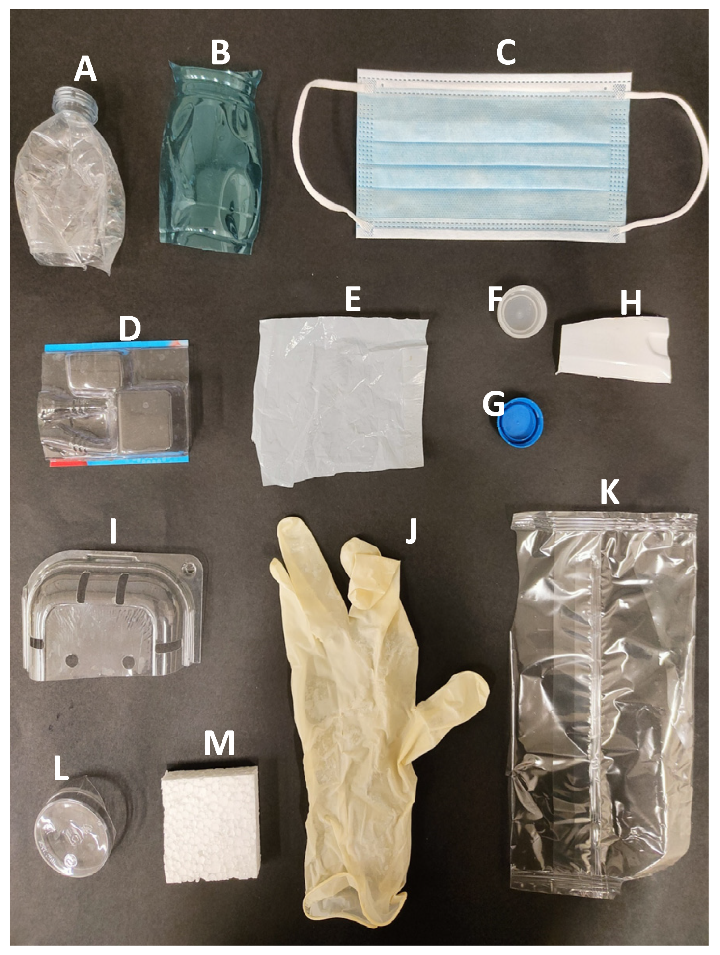
Figure 2.
Experimental set-up in the laboratory for the fluorescence LIDAR experiments: (a) block diagram of the experimental set-up, (b) detail of the 45° mirror and the container filled with water, and (c) photo of the laser-induced fluorescence emitted from dissolved organic matter present in the water column and from the plastic bottle when hit by the laser beam.
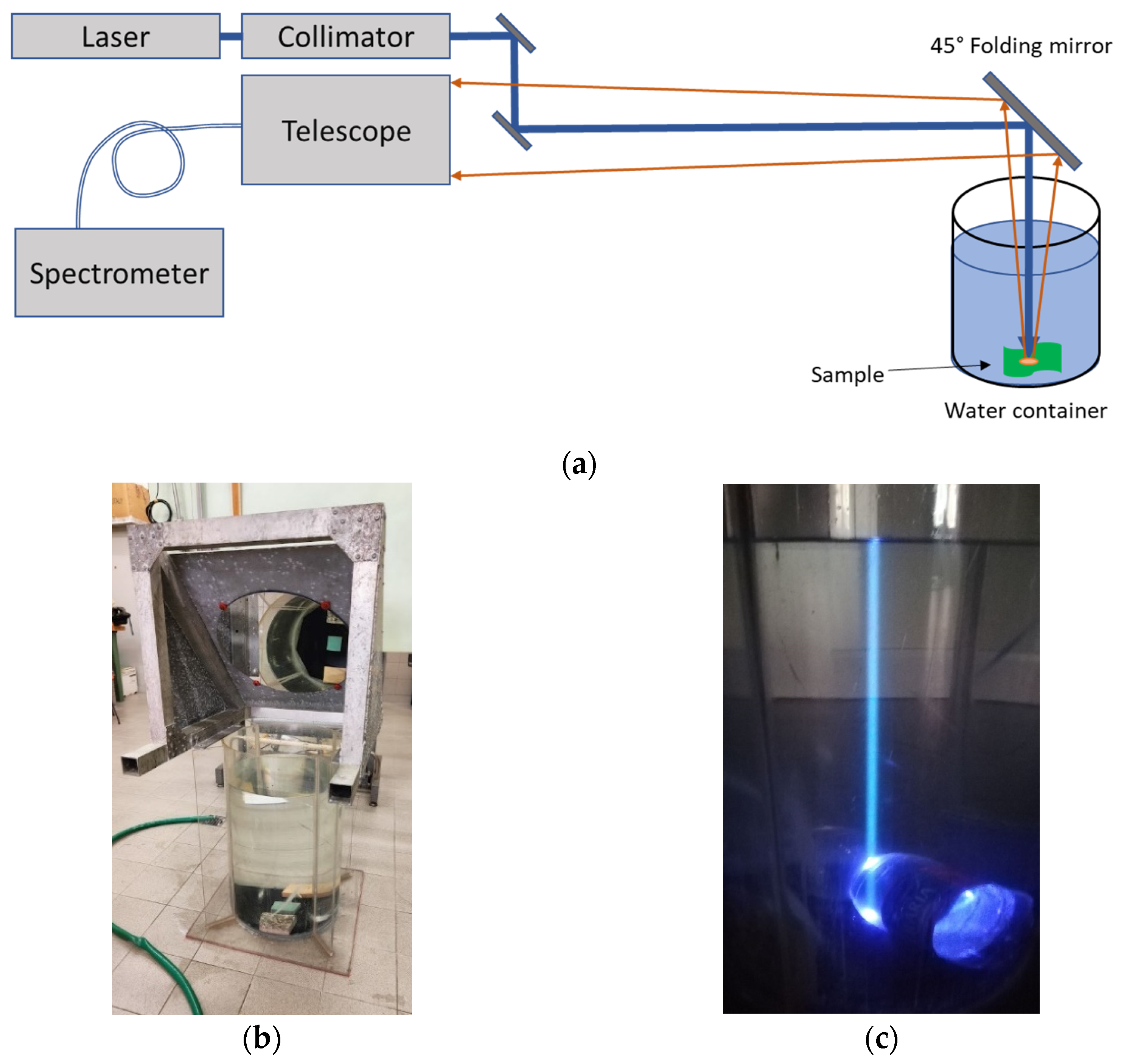
Figure 3.
Fluorescence LIDAR spectra of the dry plastic samples: (a) fluorescence spectra of samples A, B, D, H, I, J, L; (b) fluorescence spectra of samples C, E, F, G, K, M; (c) fluorescence spectra of samples A, B, D, H, I, J, L, normalized to the standard deviation (STD), and (d) fluorescence spectra of samples C, E, F, G, K, M, normalized to the standard deviation (STD).
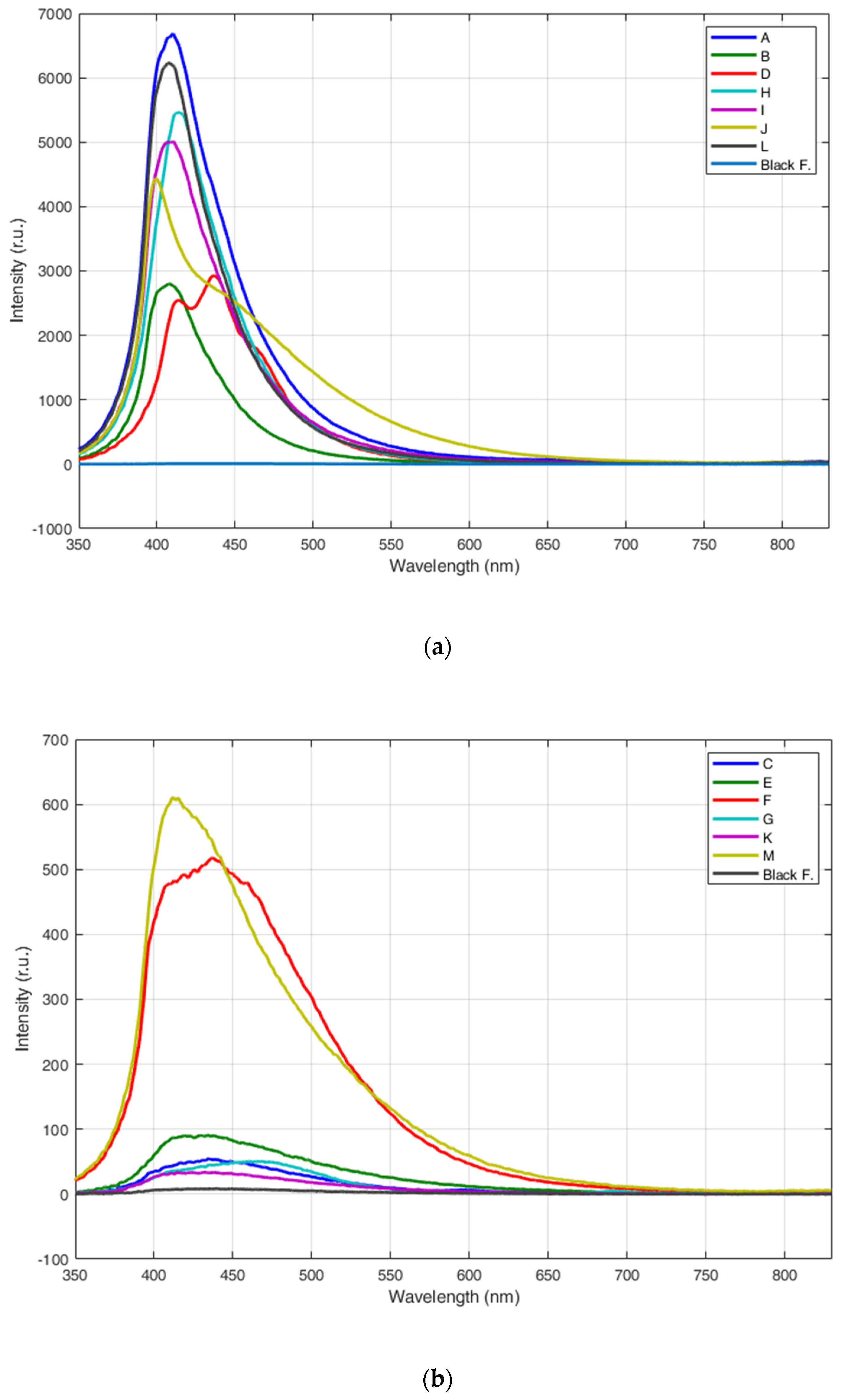
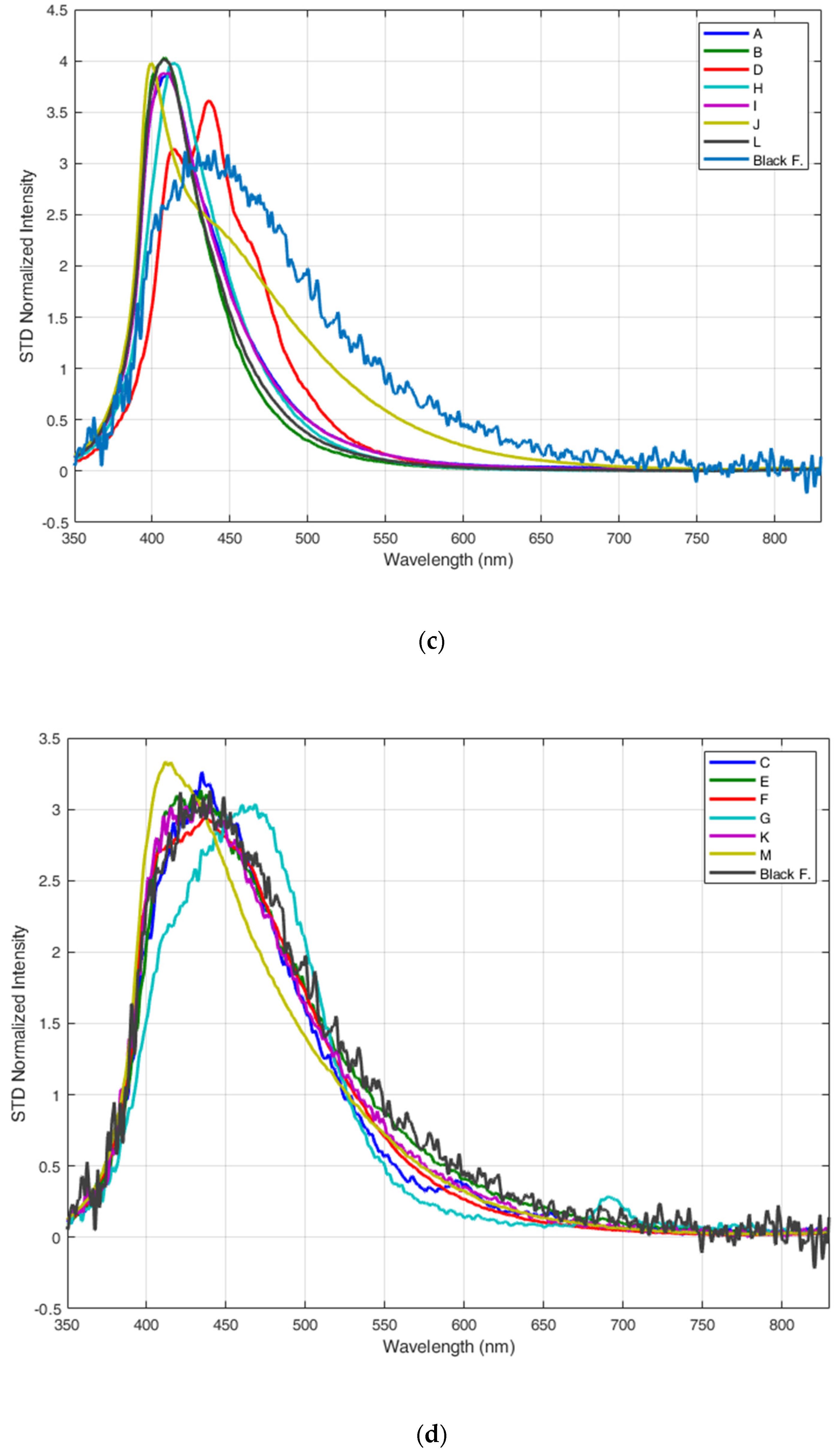
Figure 4.
Fluorescence LIDAR spectra of a 50 cm high water column (blue line) and of the background (Black F—black foil at the bottom of the empty container—green line).
Figure 4.
Fluorescence LIDAR spectra of a 50 cm high water column (blue line) and of the background (Black F—black foil at the bottom of the empty container—green line).

Figure 5.
Fluorescence LIDAR spectra of samples A through L immersed in a 50 cm water column and, for comparison, the fluorescence LIDAR spectrum of the 50 cm water column (dashed cyan line).
Figure 5.
Fluorescence LIDAR spectra of samples A through L immersed in a 50 cm water column and, for comparison, the fluorescence LIDAR spectrum of the 50 cm water column (dashed cyan line).
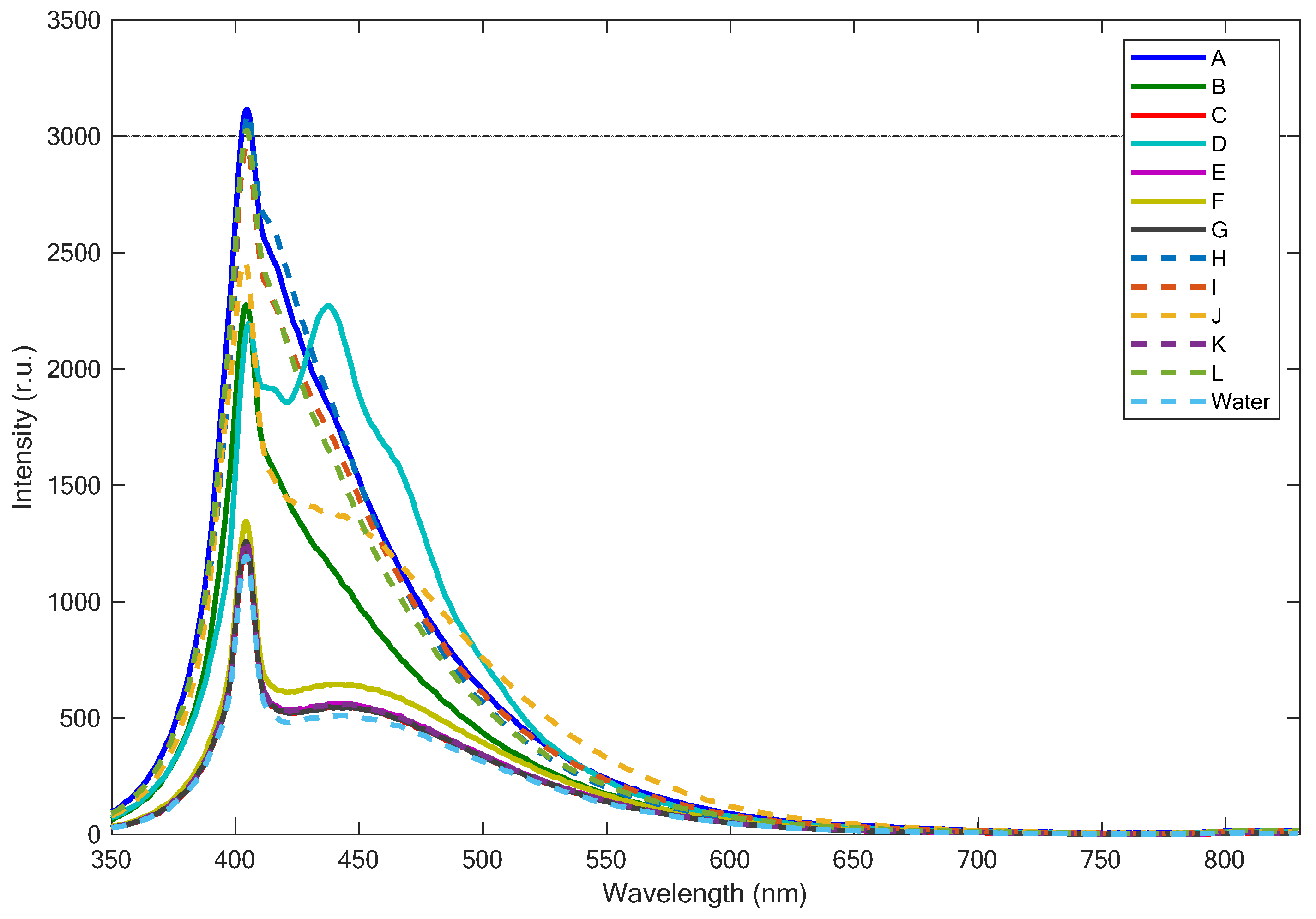
Figure 6.
Corrected fluorescence spectra retrieved from the spectra acquired on the wet samples (green lines) and the corresponding spectra acquired on the dry samples (blue lines): (A) transparent PET bottle, (B) blue PET bottle, (C) surgical mask, (D) transparent blister, (E) white plastic bag, (F) white bottle cap, (G) blue bottle cap, (H) white bottle, (I) fresh fruit container, (J) latex glove, (K) transparent packaging, (L) transparent plastic glass.

Figure 7.
Fluorescence LIDAR spectra of the other materials that can be typically found as marine debris: (a) leaf, (b) wood log, and (c) relevant fluorescence spectra (wood heart, wood bark, leaf) together with a typical fluorescence spectrum of (mesotrophic) sea waters. For the sake of clarity, one spectrum acquired on the leaf was multiplied by a 10 factor (in order to see the chlorophyll fluorescence spectral shape) and sea water spectrum by a 0.5 factor (in order to see the Raman signal). The locations where the fluorescence measurements were acquired are marked in (a,b) with circles of the same color of the spectra in (c).

Table 1.
List of commercial plastic samples.
| Name | Description | Material | Thickness (µm) |
|---|---|---|---|
| A | Transparent Bottle | Polyethylene terephthalate (PET) | 140 |
| B | Bluish Bottle | Polyethylene terephthalate (PET) | 180 |
| C | Surgical Mask | Polypropylene (PP) | 300 |
| D | Blister | Polyvinyl chloride (PVC) | 160 |
| E | Plastic Bag | n.a. | 30 |
| F | White Bottle Cap | High-density polyethylene (HDPE) | 550 |
| G | Blue Bottle Cap | High-density polyethylene (HDPE) | 700 |
| H | White Bottle | Polyethylene terephthalate (PET) | 600 |
| I | Fresh Fruit Container | Recycled polyethylene terephthalate (R-PET) | 260 |
| J | Surgical Glove | LATEX | 230 |
| K | Transparent Packaging | Polypropylene (PP) | 60 |
| L | Transparent Plastic Glass | Polyethylene terephthalate (PET) | 430 |
| M | Polystyrene Slab | Expanded polystyrene (EPS) | 10,000 |
Table 2.
Main technical data of the fluorescence LIDAR system.
| Parameter | Value |
|---|---|
| Laser source | 3ω Nd:YAG, Q-Switched (355 nm, 12 mJ@20 Hz, 5 ns) |
| Telescope | Newtonian (1000-mm focal length, f/4) |
| Operative distance range | from 4 m to 100 m |
| IFOV | 1 mrad |
| Spectrometer | 300 mm focal length, f/3.9 |
| Spectral range | 350–830 nm |
| Spectral resolution | 0.5 nm, 0.1 nm or 0.02 nm depending on the used grating (150 gg/mm, 600 gg/mm, 2400 gg/mm) |
| Pointing field of view | Full solid angle |
| Pointing accuracy | 25 µrad |
| Size | 100 cm × 85 cm × 75 cm (operative) |
| Weight | 35 kg + spectrometer module |
Publisher’s Note: MDPI stays neutral with regard to jurisdictional claims in published maps and institutional affiliations. |
© 2022 by the authors. Licensee MDPI, Basel, Switzerland. This article is an open access article distributed under the terms and conditions of the Creative Commons Attribution (CC BY) license (https://creativecommons.org/licenses/by/4.0/).
Share and Cite
MDPI and ACS Style
Palombi, L.; Raimondi, V. Experimental Tests for Fluorescence LIDAR Remote Sensing of Submerged Plastic Marine Litter. Remote Sens. 2022, 14, 5914. https://doi.org/10.3390/rs14235914
AMA Style
Palombi L, Raimondi V. Experimental Tests for Fluorescence LIDAR Remote Sensing of Submerged Plastic Marine Litter. Remote Sensing. 2022; 14(23):5914. https://doi.org/10.3390/rs14235914
Chicago/Turabian StylePalombi, Lorenzo, and Valentina Raimondi. 2022. "Experimental Tests for Fluorescence LIDAR Remote Sensing of Submerged Plastic Marine Litter" Remote Sensing 14, no. 23: 5914. https://doi.org/10.3390/rs14235914
Note that from the first issue of 2016, this journal uses article numbers instead of page numbers. See further details here.