
An Integrated Approach to Map the Impact of Climate Change on the Distributions of Crataegus azarolus and Crataegus monogyna in Kurdistan Region, Iraq


Abstract
1. Introduction
2. Materials and Methods
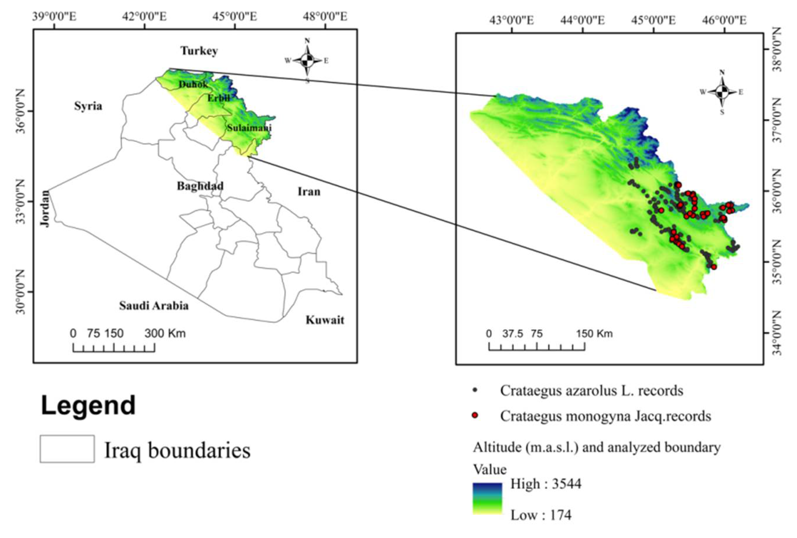
2.1. Study Area
2.2. Species Occurrence Data Collection
2.3. Environmental Data Sources
2.4. Model Building
2.5. Model Evaluation
2.6. Current and Future Habitat Distributions Change Analysis for the Species
3. Results
3.1. The Model’s Performance
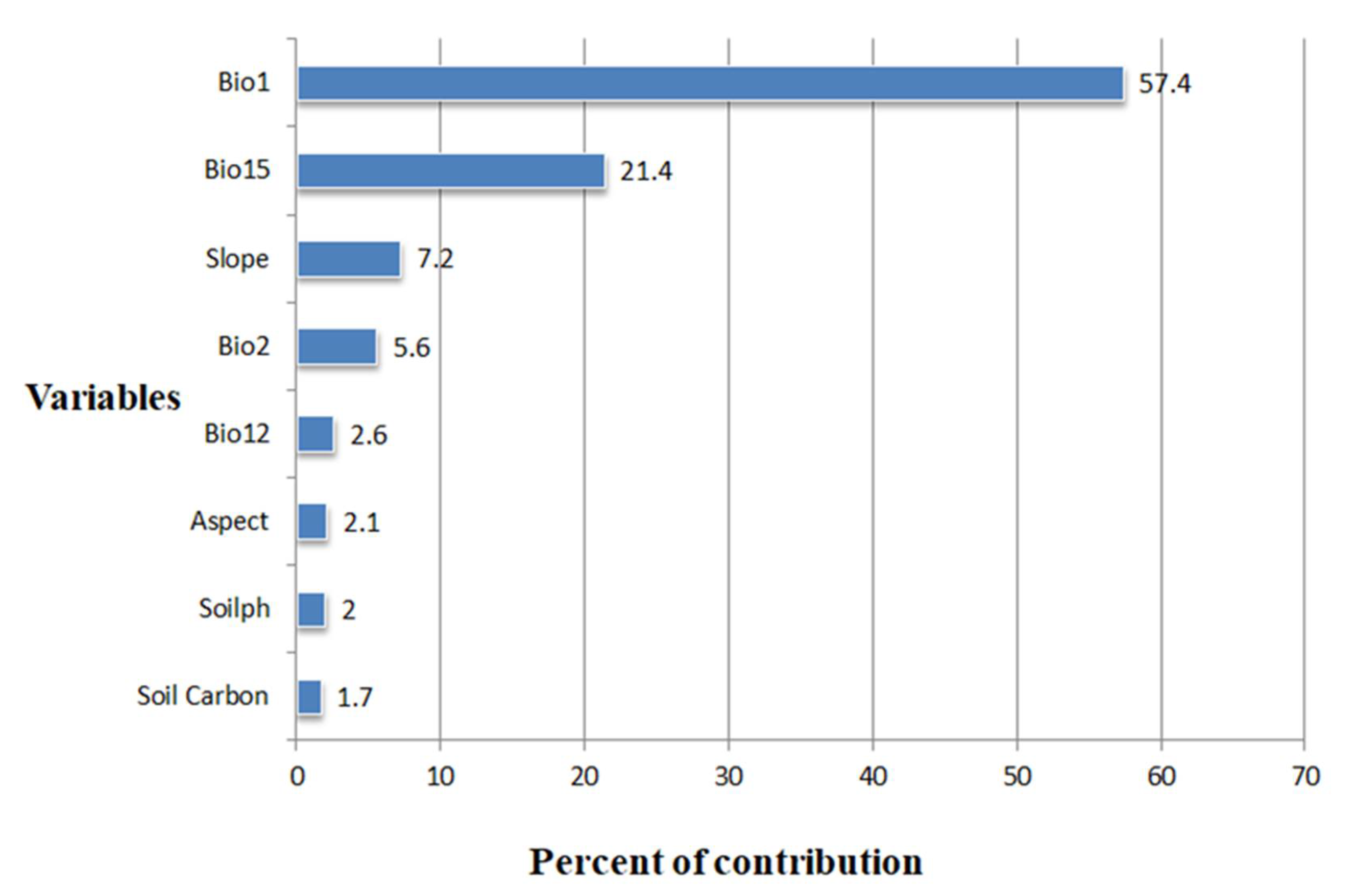
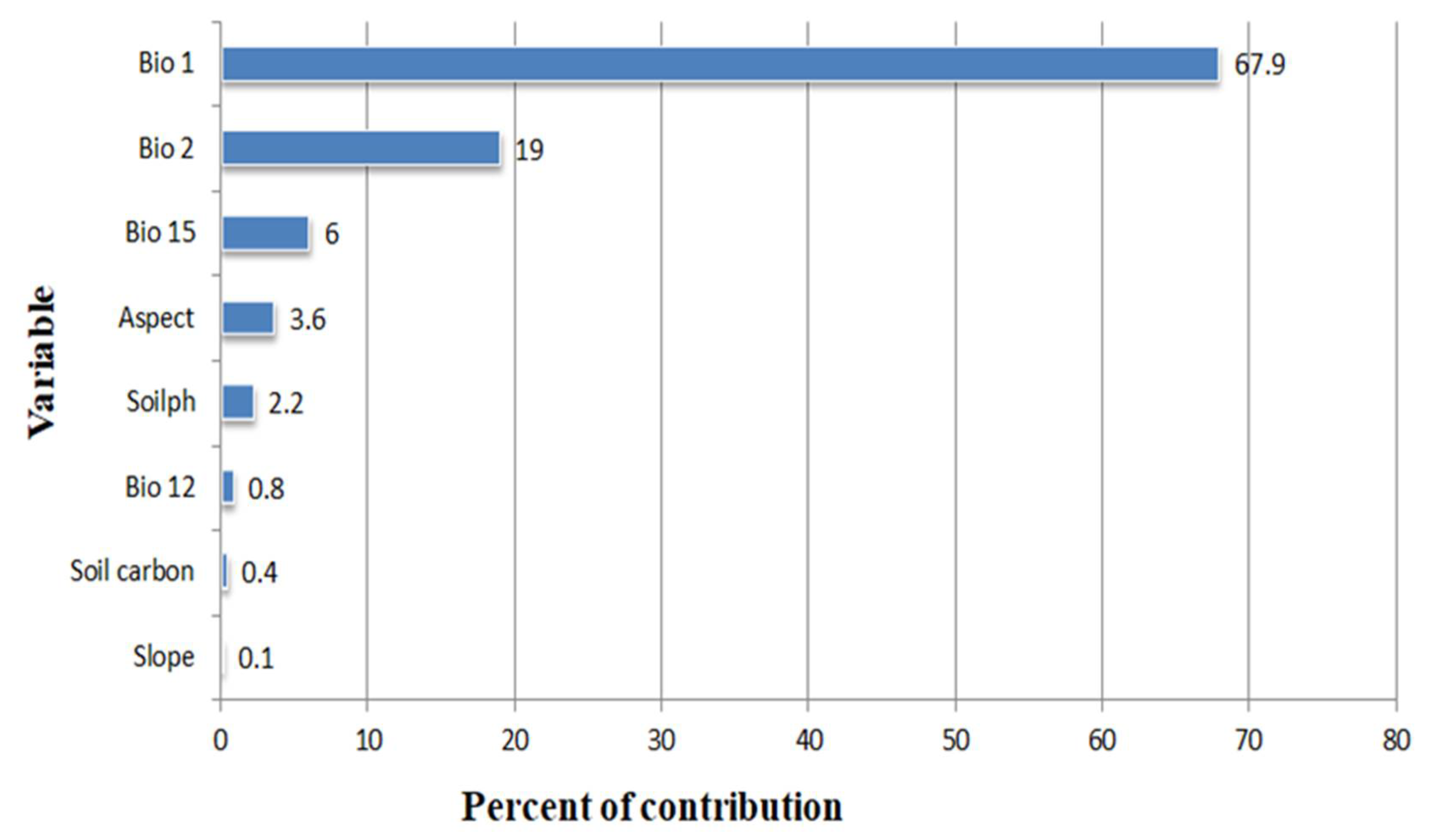
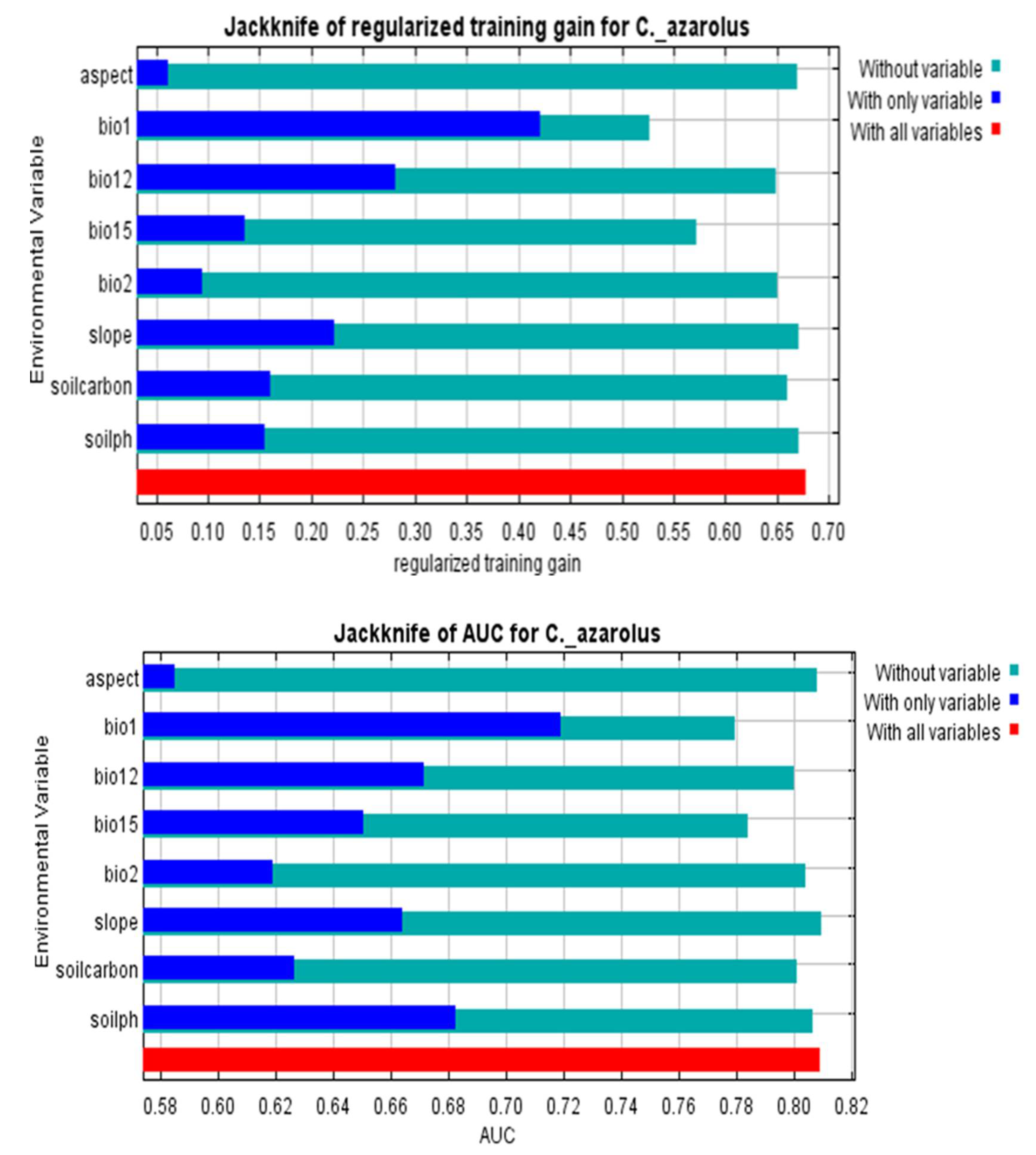
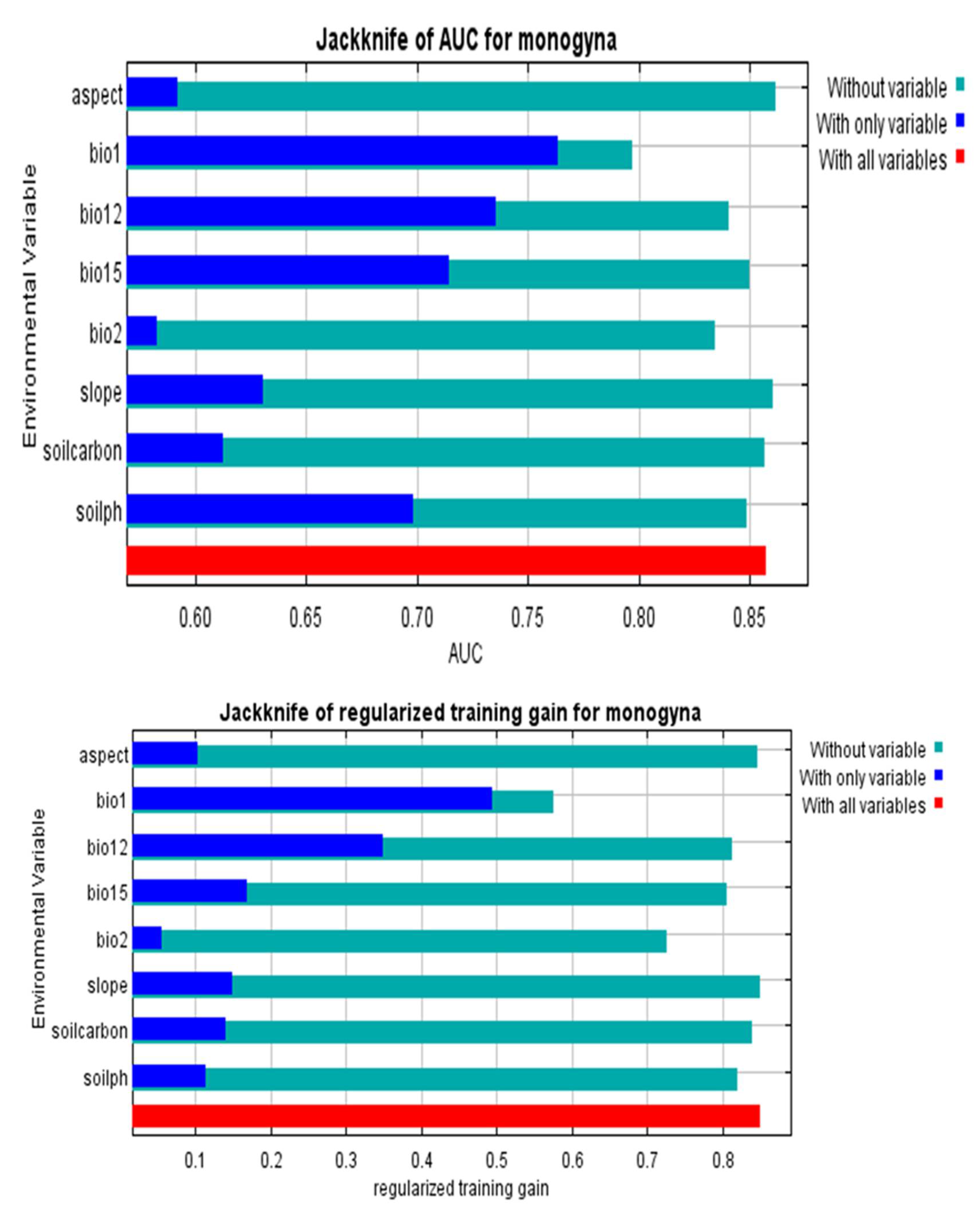
3.2. Determinants of C. monogyna and C. azarolus Distributions
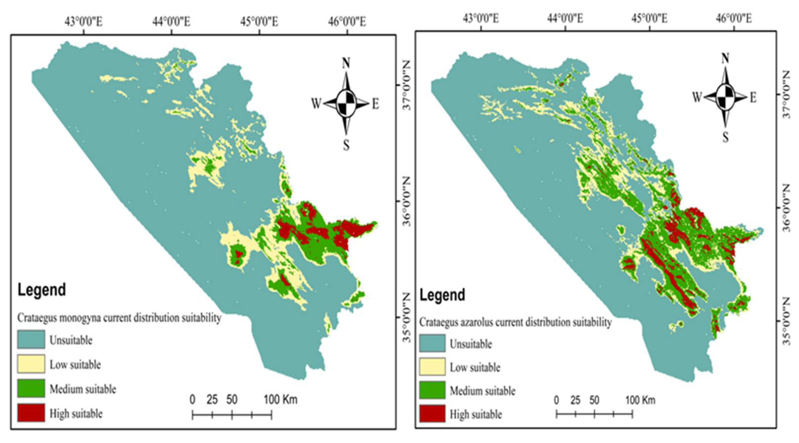
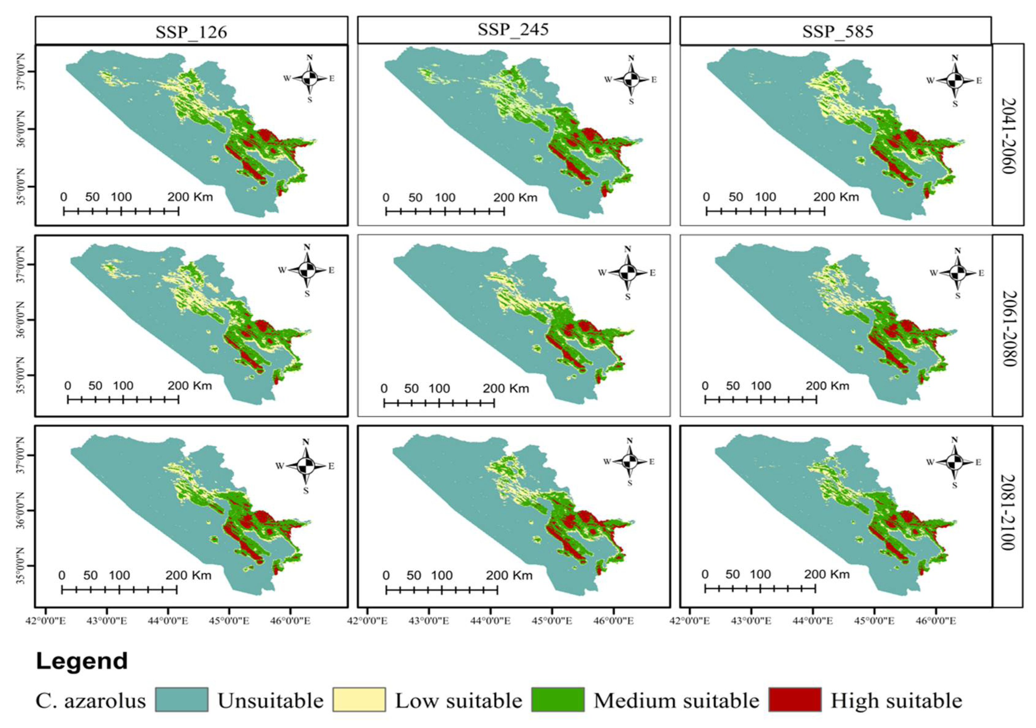
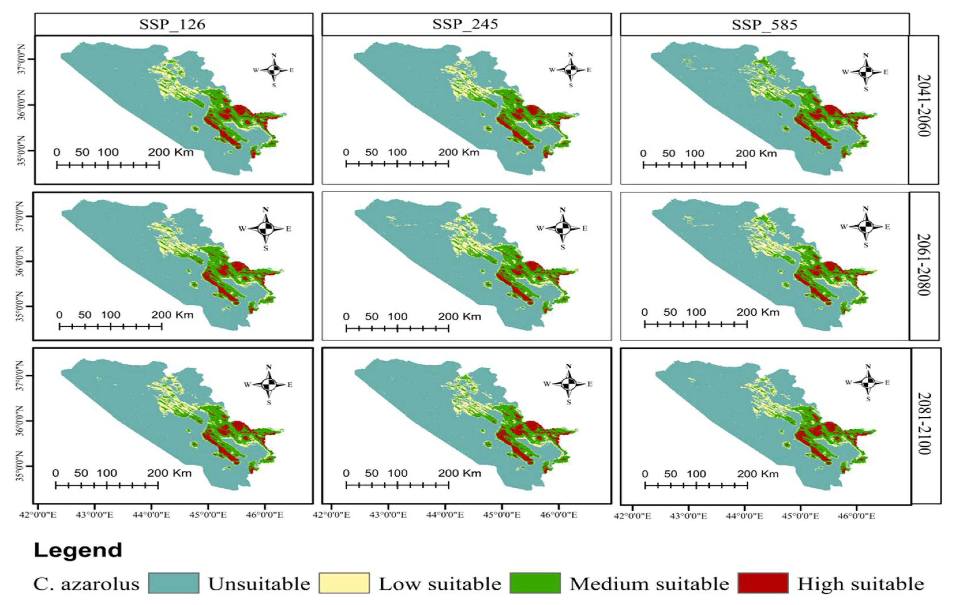
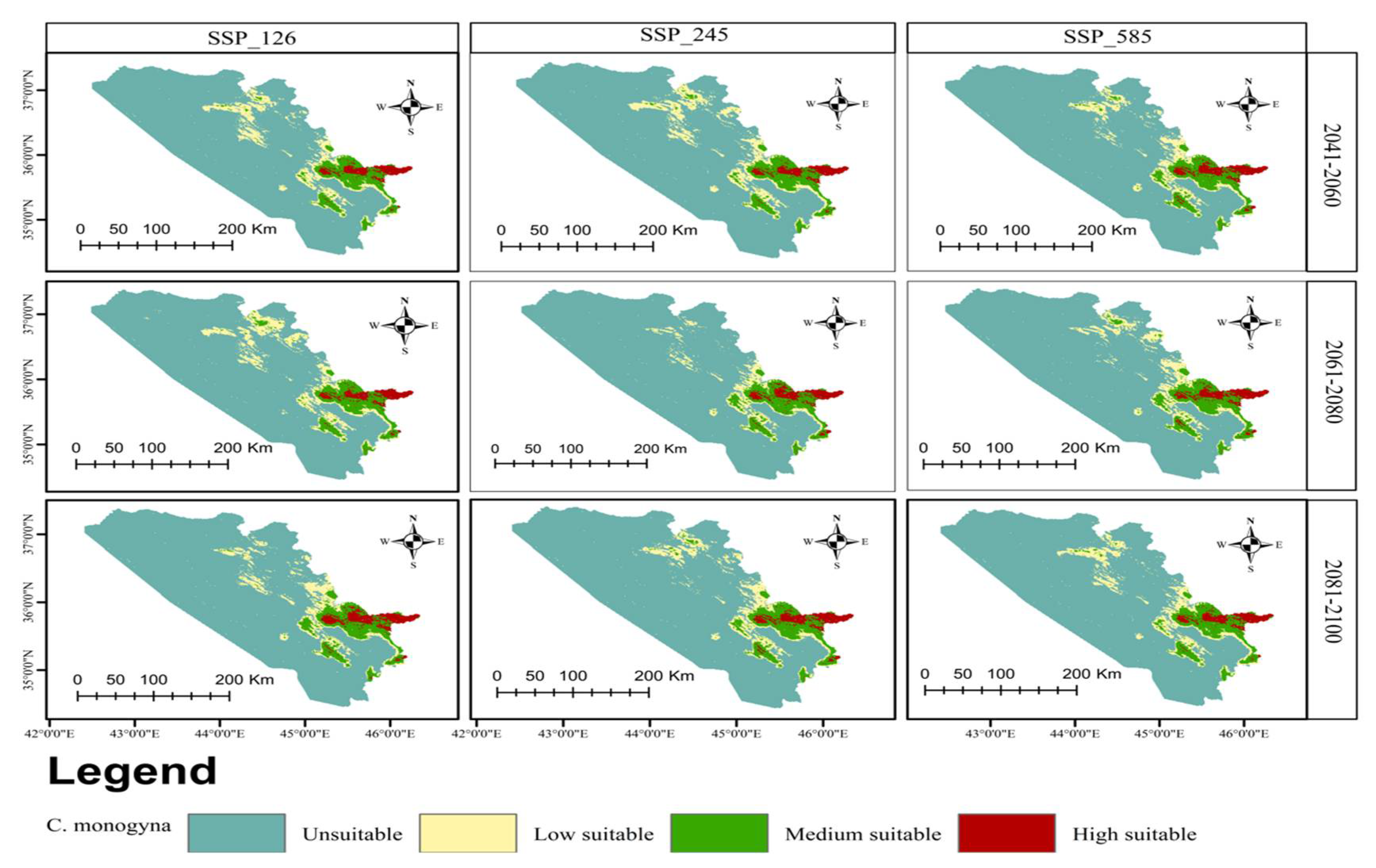
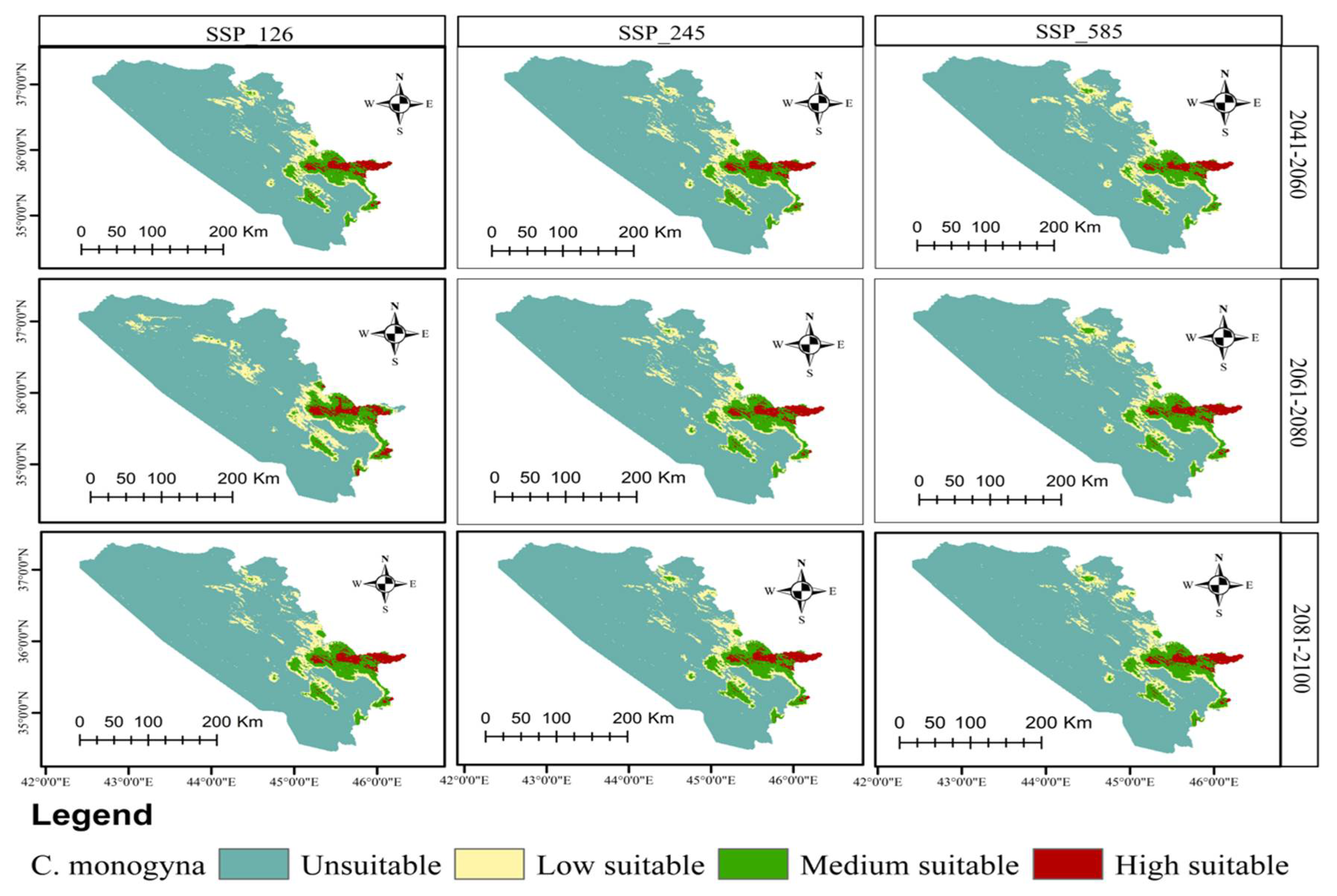
3.3. Current and Future Distributions of C. monogyna and C. azarolus
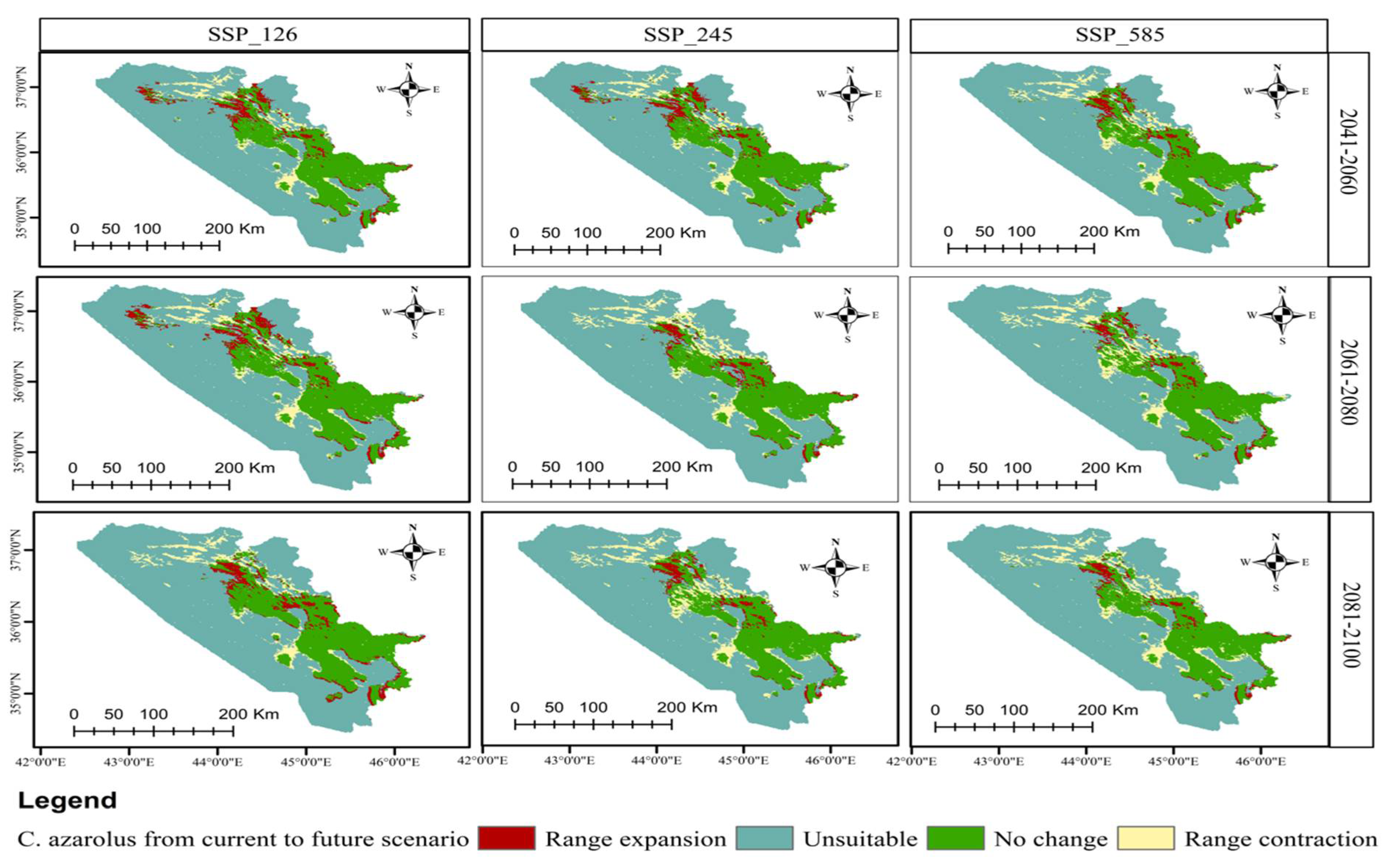
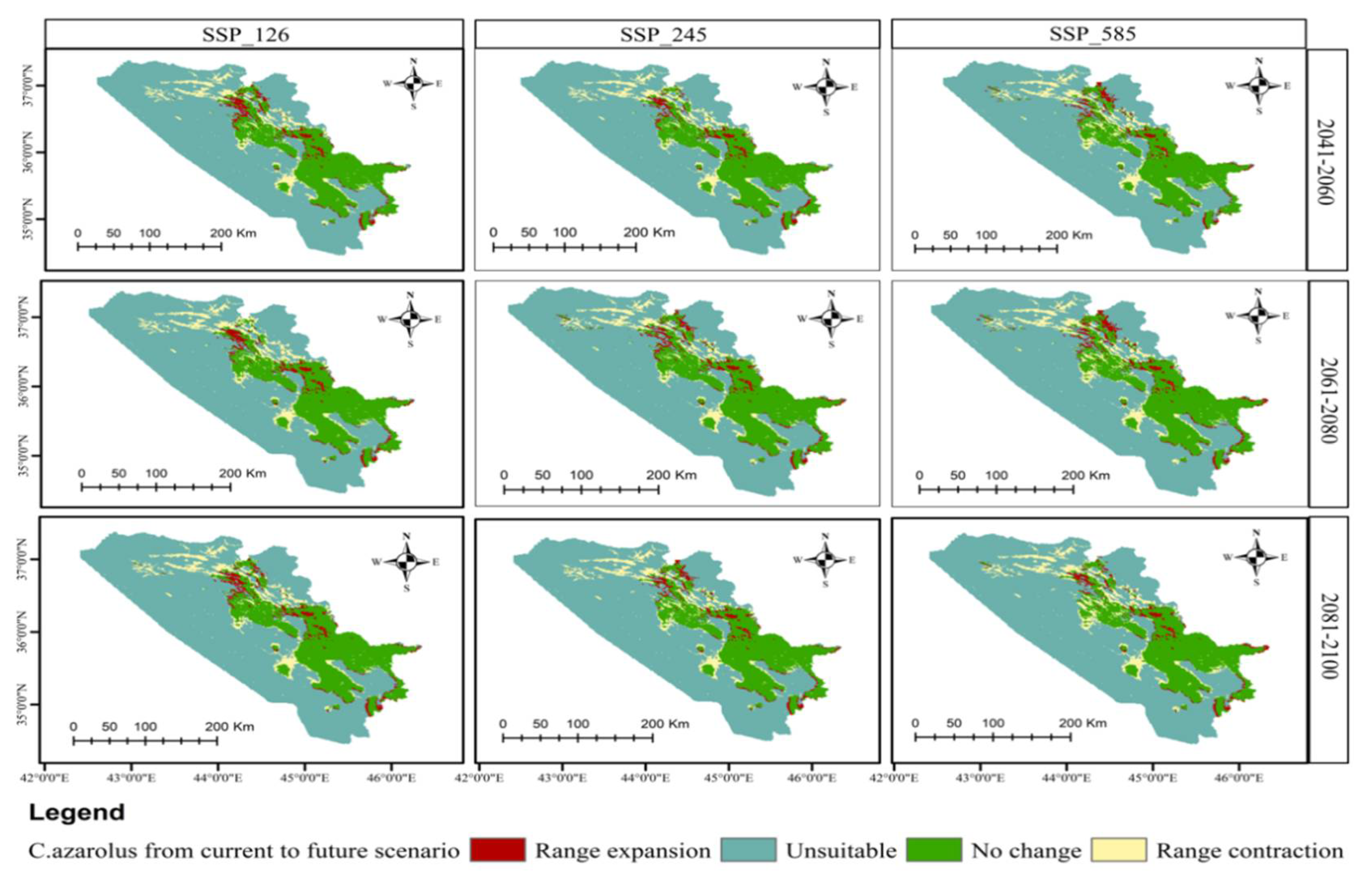
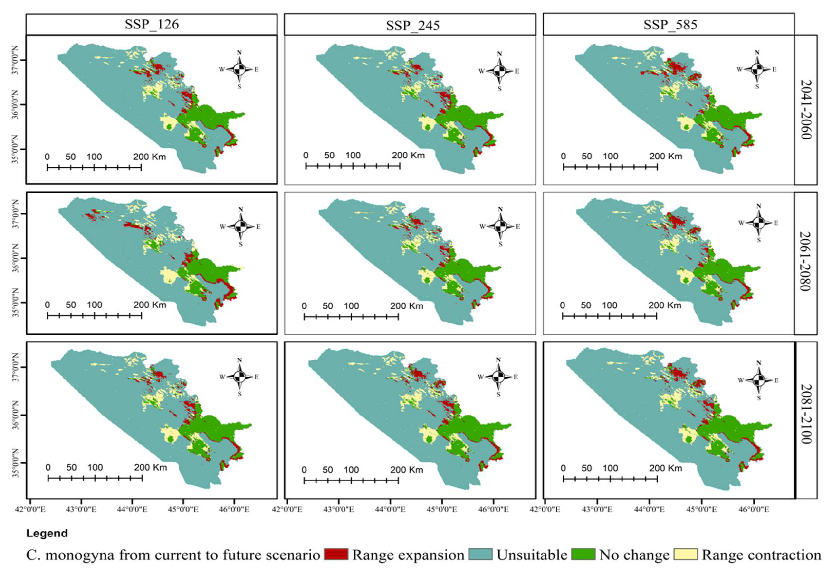
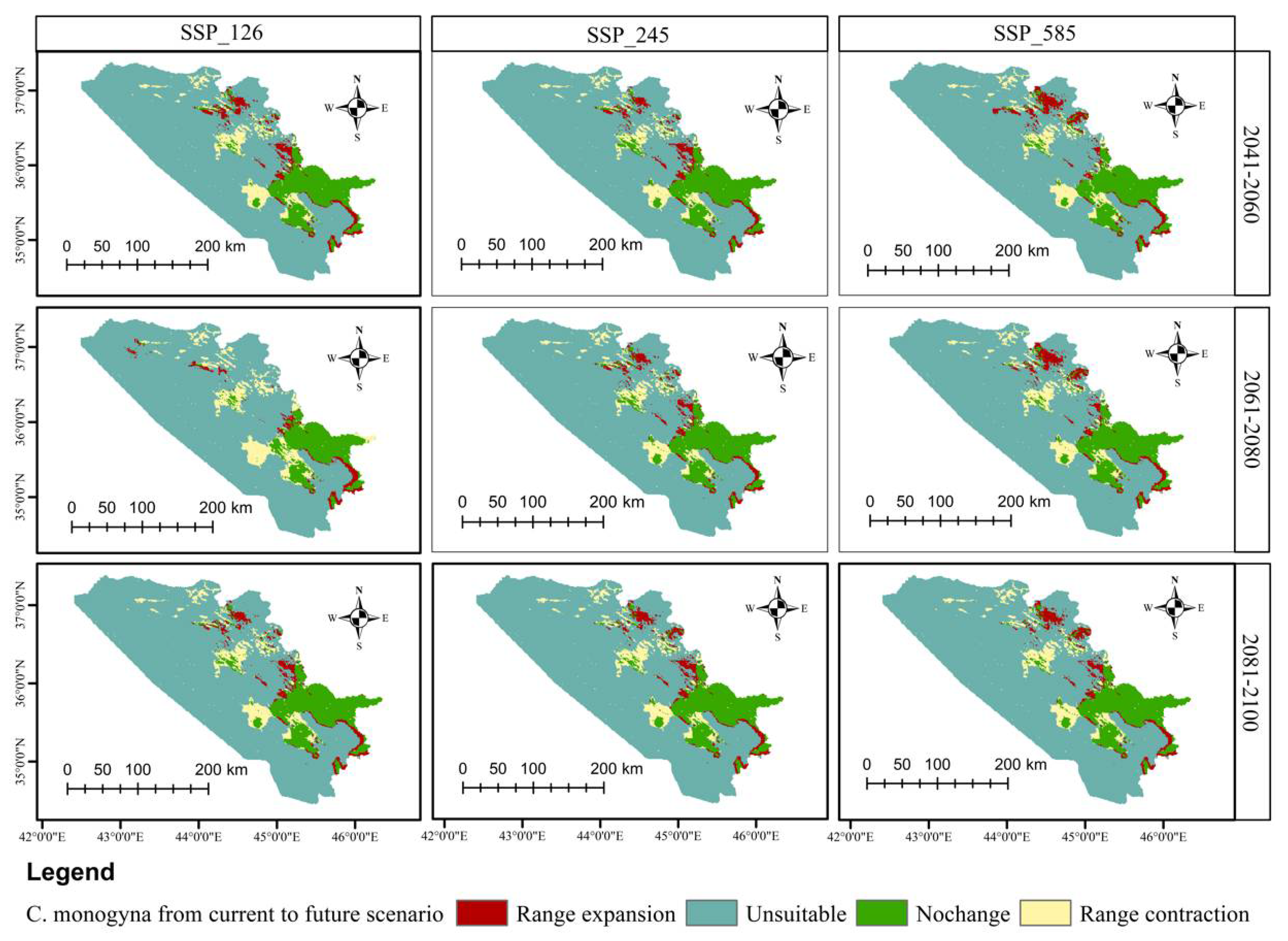
3.4. Distribution Change Analysis between Current and Future Habitat for C. azarolus and C. monogyna
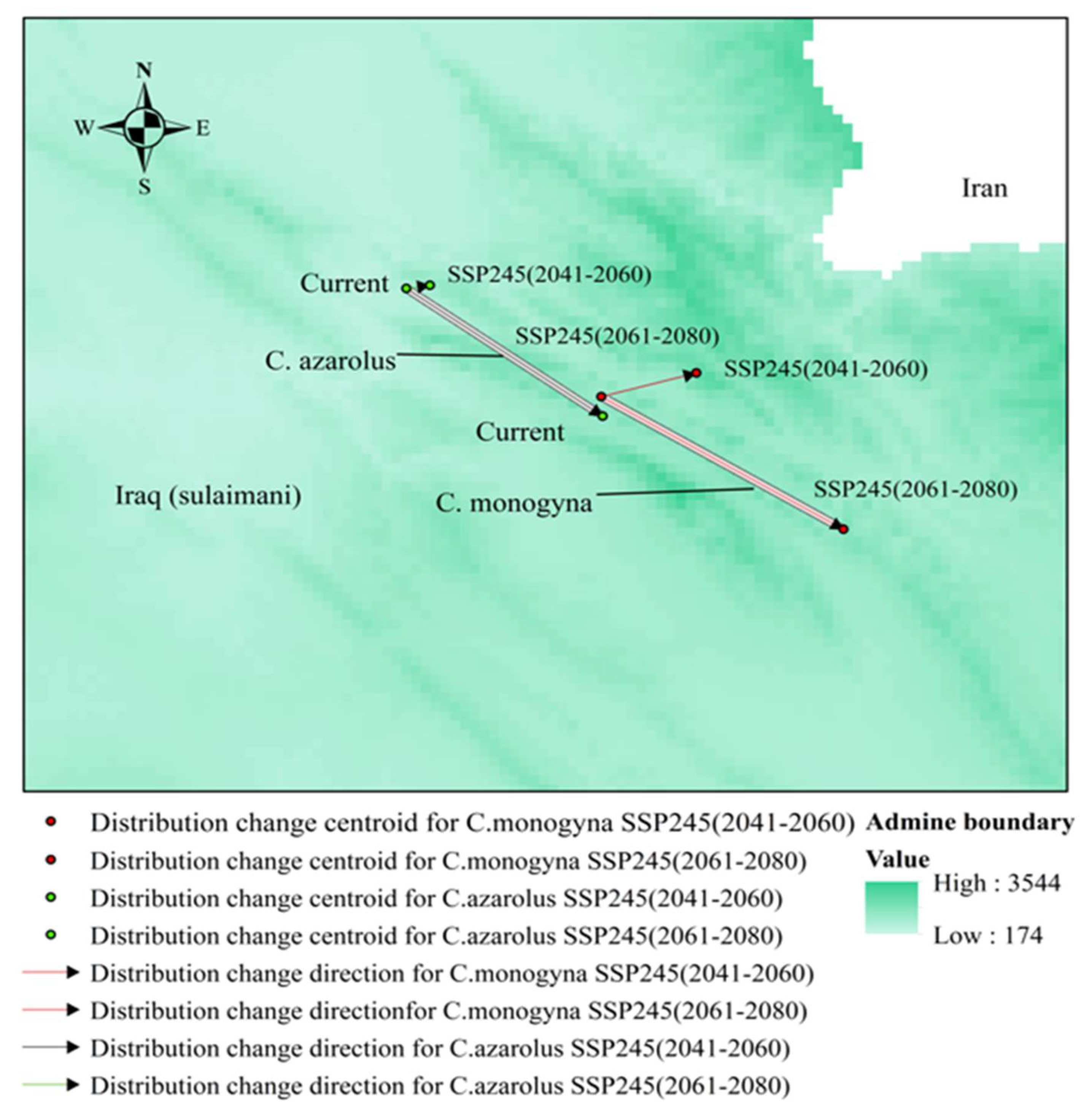
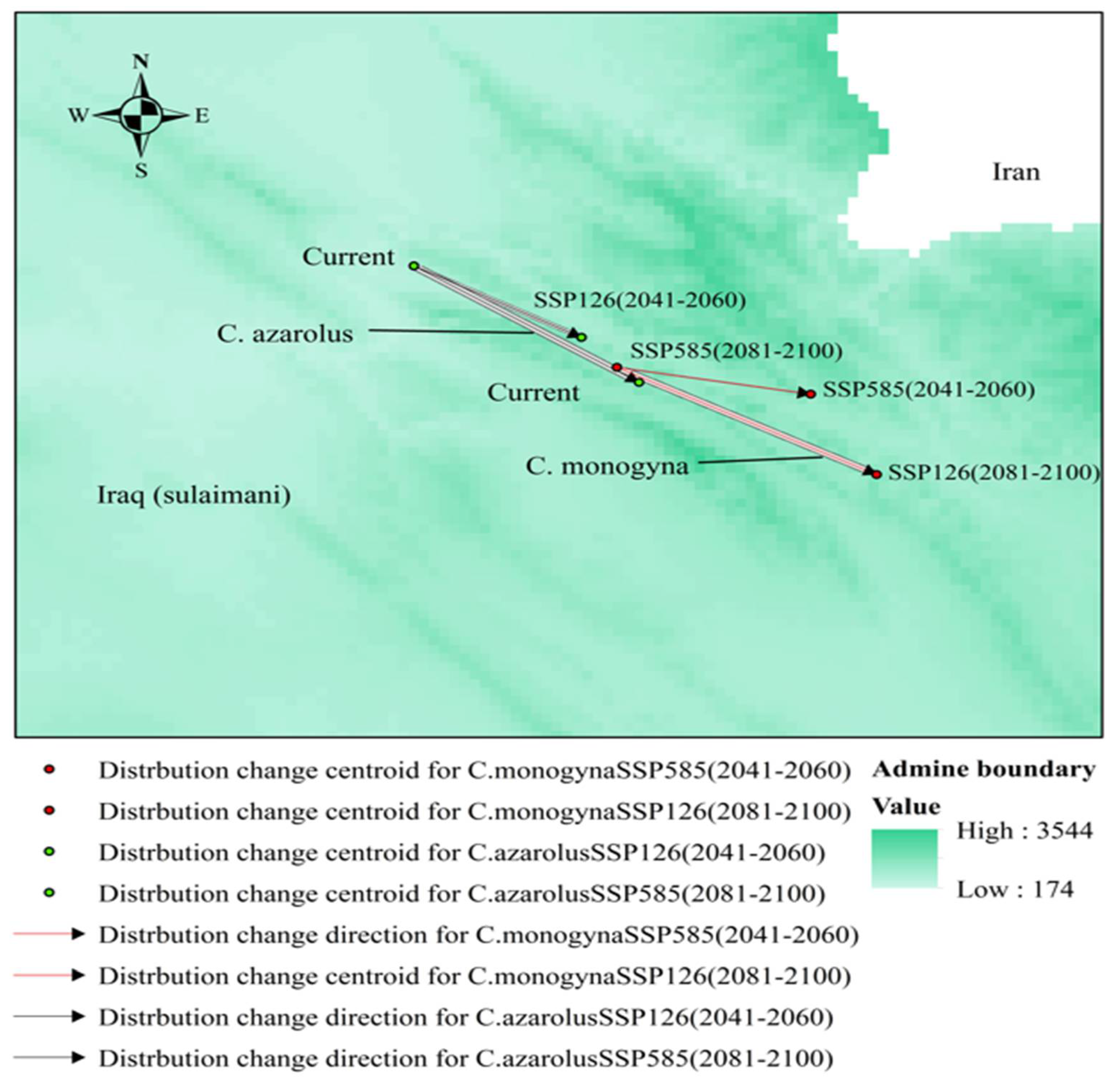
3.5. Distributional Change Direction and Migration of Geographical Patterns for C. azarolus and C. monogyna under Future Changes in Climate
4. Discussion
4.1. Distribution of C. azarolus and C. monogyna Undercurrent and Future Climate Conditions
4.2. Environmental Variables Controlling the Distribution of C. monogyna and C. azarolus
4.3. Implications for Conservation
5. Conclusions
Author Contributions
Funding
Institutional Review Board Statement
Informed Consent Statement
Data Availability Statement
Acknowledgments
Conflicts of Interest
Appendix A


| Variables | Code and Unit |
|---|---|
| Annual mean temperature | Bio1 (°C) |
| Mean diurnal range | Bio2 (°C) |
| Isothermality (Bio2/Bio7) | Bio3 (×100) |
| Temperature seasonality | Bio4 (standard deviation × 100) |
| Max temperature of warmest month | Bio5 (°C) |
| Min temperature of coldest month | Bio6 (°C) |
| Temperature annual range | Bio7 (Bio5-Bio6) (°C) |
| Mean temperature of wettest quarter | Bio8 (°C) |
| Mean temperature of driest quarter | Bio9 (°C) |
| Mean temperature of warmest quarter | Bio10 (°C) |
| Mean temperature of coldest quarter | Bio11 (°C) |
| Annual precipitation | Bio12 (mm) |
| Precipitation of wettest month | Bio13 (mm) |
| Precipitation of driest month | Bio14 (mm) |
| Precipitation seasonality (coefficient of variation) | Bio15 (mm) |
| Precipitation of wettest quarter | Bio16 (mm) |
| Precipitation of driest quarter | Bio17 (mm) |
| Precipitation of warmest quarter | Bio18 (mm) |
| Precipitation of coldest quarter | Bio19 (mm) |
| Slope | Slope (degree) |
| Aspect | Aspect (degree) |
| Soil pH | Soil (parts hydrogen) |
| Soil carbon | gm·kg−1 |
| Soil moisture | Soil moisture (mm) |


References
- Christensen, K.I. Revision of Crataegus sect. Crataegus and Nothosect. Crataeguineae (Rosaceae-Maloideae) in the old world. Syst. Bot. Monogr. 1992, 35, 1–199. [Google Scholar] [CrossRef]
- Özcan, M.; Hacıseferoğulları, H.; Marakoğlu, T.; Arslan, D. Hawthorn (Crataegus spp.) fruit: Some physical and chemical properties. J. Food Eng. 2005, 69, 409–413. [Google Scholar] [CrossRef]
- Naghipour, A.A.; Asl, S.T.; Ashrafzadeh, M.R.; Haidarian, M. Predicting the Potential Distribution of Crataegus azarolus L. under Climate Change in Central Zagros, Iran. J. Wildl. Biodivers. 2021, 5, 28–43. [Google Scholar]
- Zeravan, A.S.; Shahbaz, S.I.; AL Maa, A.M. Numerical Taxonomy for Genus Crataegus L. (Rosaceae) in North of Iraq. Rafidain J. Sci. 2007, 18, 1–15. [Google Scholar]
- Gurlen, A.; Gundogdu, M.; Ozer, G.; Ercisli, S.; Duralija, B. Primary, secondary metabolites and molecular characterization of hawthorn (Crataegus spp.) genotypes. Agronomy 2020, 10, 1731. [Google Scholar] [CrossRef]
- Shahbaz, S.E.; Sadeq, Z.A. Crataegus azarolus var. sharania (Rosaceae), a new variety for the flora of Iraq. Nord. J. Bot. 2003, 23, 713–717. [Google Scholar] [CrossRef]
- Saadatian, M.; Peshawa, F.; Asiaban, K.; Karzan, A.; Muhammad, H. Determination of biochemical content and some pomological characteristics of 4 Hawthorn species (Crataegus spp.) grown in Erbil Province, Kregion, Iraq. Adv. Environ. Biol. 2014, 8, 2465–2469. [Google Scholar]
- Al-Ansari, N. Topography and climate of Iraq. J. Earth Sci. Geotech. Eng. 2021, 11, 1–13. [Google Scholar] [CrossRef]
- Khwarahm, N.R. Mapping current and potential future distributions of the oak tree (Quercus aegilops) in the Kurdistan Region, Iraq. Ecol. Process. 2020, 9, 56. [Google Scholar] [CrossRef]
- Ahmadloo, F.; Kochaksaraei, M.T.; Azadi, P.; Hamidi, A.; Beiramizadeh, E. Effects of pectinase, BAP and dry storage on dormancy breaking and emergence rate of Crataegus pseudoheterophylla Pojark. New For. 2015, 46, 373–386. [Google Scholar] [CrossRef]
- Nazhand, A.; Lucarini, M.; Durazzo, A.; Zaccardelli, M.; Cristarella, S.; Souto, S.B.; Silva, A.M.; Severino, P.; Souto, E.B.; Santini, A. Hawthorn (Crataegus spp.): An updated overview on its beneficial properties. Forests 2020, 11, 564. [Google Scholar] [CrossRef]
- Özyurt, G.; Yücesan, Z.; Ak, N.; Oktan, E.; Üçler, A. Ecological and economic importance of studying propagation techniques of common hawthorn Crataegus monogyna Jacq. Cибиpcкий Лecнoй Жypнaл 2019, 4, 63–67. [Google Scholar]
- Khwarahm, N.R. Spatial modeling of land use and land cover change in Sulaimani, Iraq, using multitemporal satellite data. Environ. Monit. Assess. 2021, 193, 1–18. [Google Scholar] [CrossRef] [PubMed]
- Nasser, M. Forests and forestry in Iraq: Prospects and limitations. Commonw. For. Rev. 1984, 63, 299–304. [Google Scholar]
- Khwarahm, N.R. Modeling forest-shrubland fire susceptibility based on machine learning and geospatial approaches in mountains of Kurdistan Region, Iraq. Arab. J. Geosci. 2022, 15, 1–17. [Google Scholar] [CrossRef]
- Adamo, N.; Al-Ansari, N.; Sissakian, V.; Fahmi, K.J.; Ali Abed, S. Climate Change: Droughts and Increasing Desertification in the Middle East, with Special Reference to Iraq. Engineering 2022, 14, 235–273. [Google Scholar] [CrossRef]
- Alnasrawi, A. Iraq: Economic sanctions and consequences, 1990–2000. Third World Q. 2001, 22, 205–218. [Google Scholar] [CrossRef]
- Monzón, J.; Moyer-Horner, L.; Palamar, M.B. Climate change and species range dynamics in protected areas. Bioscience 2011, 61, 752–761. [Google Scholar] [CrossRef]
- Balaky, H.H.; Khalid, K.; Hasan, A.; Tahir, S.; Sedat, U.; Khedir, A. Estimation of total tannin and total phenolic content in plant (Crataegus azarolus L.) by orbital shaker technique. Int. J. Agric. Environ. Food Sci. 2021, 5, 1–6. [Google Scholar] [CrossRef]
- Mahmud, S.A.; Al-Habib, O.A.; Bugoni, S.; Clericuzio, M.; Vidari, G. A new ursane-type triterpenoid and other constituents from the leaves of Crataegus azarolus var. aronia. Nat. Prod. Commun. 2016, 11, 1934578X1601101103. [Google Scholar] [CrossRef]
- Beigmohamadi, M.; Rahmani, F.; Mirzaei, L. Study of Genetic Diversity Among Crataegus Species (Hawthorn) Using ISSR Markers in Northwestern of Iran. Pharm. Biomed. Res. 2021, 7, 59–66. [Google Scholar] [CrossRef]
- Khadivi-Khub, A.; Karimi, S.; Kameli, M. Morphological diversity of naturally grown Crataegus monogyna (Rosaceae, Maloideae) in Central Iran. Braz. J. Bot. 2015, 38, 921–936. [Google Scholar] [CrossRef]
- Moustafa, A.; Zaghloul, M.; Mansour, S.; Alotaibi, M. Conservation Strategy for protecting Crataegus x sinaica against climate change and anthropologic activities in South Sinai Mountains, Egypt. Catrina Int. J. Environ. Sci. 2019, 18, 1–6. [Google Scholar] [CrossRef]
- Yanar, M.; Ercisli, S.; Yilmaz, K.; Sahiner, H.; Taskin, T.; Zengin, Y.; Akgul, I.; Celik, F. Morphological and chemical diversity among hawthorn (Crataegus spp.) genotypes from Turkey. Sci. Res. Essays 2011, 6, 35–38. [Google Scholar]
- Hu, G.; Wang, Y.; Wang, Y.; Zheng, S.; Dong, W.; Dong, N. New insight into the phylogeny and taxonomy of cultivated and related species of Crataegus in China, based on complete chloroplast genome sequencing. Horticulturae 2021, 7, 301. [Google Scholar] [CrossRef]
- Du, X.; Zhang, X.; Bu, H.; Zhang, T.; Lao, Y.; Dong, W. Molecular analysis of evolution and origins of cultivated hawthorn (Crataegus spp.) and related species in China. Front. Plant Sci. 2019, 10, 443. [Google Scholar] [CrossRef] [PubMed]
- Hu, G.; Zheng, S.; Pan, Q.; Dong, N. The complete chloroplast genome of Crataegus hupehensis Sarg. (Rosaceae), a medicinal and edible plant in China. Mitochondrial DNA Part B 2021, 6, 315–317. [Google Scholar] [CrossRef]
- Lyons, M.P.; Kozak, K.H. Vanishing islands in the sky? A comparison of correlation-and mechanism-based forecasts of range dynamics for montane salamanders under climate change. Ecography 2020, 43, 481–493. [Google Scholar] [CrossRef]
- Di Pasquale, G.; Saracino, A.; Bosso, L.; Russo, D.; Moroni, A.; Bonanomi, G.; Allevato, E. Coastal pine-oak glacial refugia in the Mediterranean basin: A biogeographic approach based on charcoal analysis and spatial modelling. Forests 2020, 11, 673. [Google Scholar] [CrossRef]
- Elith, J.; Leathwick, J.R. Species distribution models: Ecological explanation and prediction across space and time. Annu. Rev. Ecol. Evol. Syst. 2009, 40, 677–697. [Google Scholar] [CrossRef]
- Franklin, J. Mapping Species Distributions: Spatial Inference and Prediction; Cambridge University Press: Cambridge, UK, 2010. [Google Scholar]
- Elith, J.; Phillips, S.J.; Hastie, T.; Dudík, M.; Chee, Y.E.; Yates, C.J. A statistical explanation of MaxEnt for ecologists. Divers. Distrib. 2011, 17, 43–57. [Google Scholar] [CrossRef]
- Phillips, S.J.; Anderson, R.P.; Schapire, R.E. Maximum entropy modeling of species geographic distributions. Ecol. Model. 2006, 190, 231–259. [Google Scholar] [CrossRef]
- Støa, B.; Halvorsen, R.; Stokland, J.N.; Gusarov, V.I. How much is enough? Influence of number of presence observations on the performance of species distribution models. Sommerfeltia 2019, 39, 1–28. [Google Scholar] [CrossRef]
- Phillips, S.J.; Dudík, M. Modeling of species distributions with Maxent: New extensions and a comprehensive evaluation. Ecography 2008, 31, 161–175. [Google Scholar] [CrossRef]
- Sissakian, V.; Jabbar, M.A.; Al-Ansari, N.; Knutsson, S. Development of Gulley Ali Beg Gorge in Rawandooz Area, Northern Iraq. Engineering 2015, 7, 16–30. [Google Scholar] [CrossRef]
- Khwarahm, N.R.; Ararat, K.; Qader, S.; Sabir, D.K. Modeling the distribution of the Near Eastern fire salamander (Salamandra infraimmaculata) and Kurdistan newt (Neurergus derjugini) under current and future climate conditions in Iraq. Ecol. Inform. 2021, 63, 101309. [Google Scholar] [CrossRef]
- Townsend, C.; Guest, E. 1985 Flora of Iraq; Ministry of Agriculture and Agrarian Reform: Baghdad, Iraq, 1966; Volume 2–8. [Google Scholar]
- Morales, N.S.; Fernández, I.C.; Baca-González, V. MaxEnt’s parameter configuration and small samples: Are we paying attention to recommendations? A systematic review. PeerJ 2017, 5, e3093. [Google Scholar] [CrossRef]
- Bhatta, K.P.; Chaudhary, R.P.; Vetaas, O.R. A comparison of systematic versus stratified-random sampling design for gradient analyses: A case study in subalpine Himalaya, Nepal. Phytocoenologia 2012, 42, 191–202. [Google Scholar] [CrossRef]
- Boakes, E.H.; McGowan, P.J.; Fuller, R.A.; Chang-qing, D.; Clark, N.E.; O’Connor, K.; Mace, G.M. Distorted views of biodiversity: Spatial and temporal bias in species occurrence data. PLoS Biol. 2010, 8, e1000385. [Google Scholar] [CrossRef]
- Moreno, J.S.; Sandoval-Arango, S.; Palacio, R.D.; Alzate, N.F.; Rincón, M.; Gil, K.; Morales, N.G.; Harding, P.; Hazzi, N.A. Distribution Models and Spatial Analyses Provide Robust Assessments of Conservation Status of Orchid Species in Colombia: The Case of Lephantes mucronata. Harv. Pap. Bot. 2020, 25, 111–121. [Google Scholar] [CrossRef]
- Boria, R.A.; Olson, L.E.; Goodman, S.M.; Anderson, R.P. Spatial filtering to reduce sampling bias can improve the performance of ecological niche models. Ecol. Model. 2014, 275, 73–77. [Google Scholar] [CrossRef]
- Brown, J.L. SDM toolbox: A python-based GIS toolkit for landscape genetic, biogeographic and species distribution model analyses. Methods Ecol. Evol. 2014, 5, 694–700. [Google Scholar] [CrossRef]
- Jafari, A.; Alipour, M.; Abbasi, M.; Soltani, A. Distribution Modeling of Hawthorn (Crataegus azarolus L.) in Chaharmahal & Bakhtiari Province Using the Maximum Entropy Method; SID: Singapore, 2019. [Google Scholar]
- Elith, J.; Kearney, M.; Phillips, S. The art of modelling range-shifting species. Methods Ecol. Evol. 2010, 1, 330–342. [Google Scholar] [CrossRef]
- Li, J.; Fan, G.; He, Y. Predicting the current and future distribution of three Coptis herbs in China under climate change conditions, using the MaxEnt model and chemical analysis. Sci. Total Environ. 2020, 698, 134141. [Google Scholar] [CrossRef] [PubMed]
- Zhang, J.; Song, M.; Li, Z.; Peng, X.; Su, S.; Li, B.; Xu, X.; Wang, W. Effects of climate change on the distribution of Akebia quinata. Predict. Manag. Clim.-Driven Range Shifts Plants 2022, 9, 752682. [Google Scholar] [CrossRef]
- Díaz, J.V.R.; González, F.d.B.J.-A.; Álvarez, P.Á.; García, M.Á.Á. Environmental niche and distribution of six deciduous tree species in the Spanish Atlantic region. Iforest-Biogeosciences For. 2014, 8, 214–221. [Google Scholar] [CrossRef]
- Pecchi, M.; Marchi, M.; Burton, V.; Giannetti, F.; Moriondo, M.; Bernetti, I.; Bindi, M.; Chirici, G. Species distribution modelling to support forest management. A literature review. Ecol. Model. 2019, 411, 108817. [Google Scholar] [CrossRef]
- Voldoire, A.; Saint-Martin, D.; Sénési, S.; Decharme, B.; Alias, A.; Chevallier, M.; Colin, J.; Guérémy, J.F.; Michou, M.; Moine, M.P. Evaluation of CMIP6 deck experiments with CNRM-CM6-1. J. Adv. Modeling Earth Syst. 2019, 11, 2177–2213. [Google Scholar] [CrossRef]
- Brzozowski, M.; Pełechaty, M.; Bogawski, P. A winner or a loser in climate change? Modelling the past, current, and future potential distributions of a rare charophyte species. Glob. Ecol. Conserv. 2022, 34, e02038. [Google Scholar] [CrossRef]
- Wu, T.; Lu, Y.; Fang, Y.; Xin, X.; Li, L.; Li, W.; Jie, W.; Zhang, J.; Liu, Y.; Zhang, L. The Beijing Climate Center climate system model (BCC-CSM): The main progress from CMIP5 to CMIP6. Geosci. Model Dev. 2019, 12, 1573–1600. [Google Scholar] [CrossRef]
- Iqbal, Z.; Shahid, S.; Ahmed, K.; Ismail, T.; Khan, N.; Virk, Z.T.; Johar, W. Evaluation of global climate models for precipitation projection in sub-Himalaya region of Pakistan. Atmos. Res. 2020, 245, 105061. [Google Scholar] [CrossRef]
- Mahmoodi, S.; Heydari, M.; Ahmadi, K.; Khwarahm, N.R.; Karami, O.; Almasieh, K.; Naderi, B.; Bernard, P.; Mosavi, A. The current and future potential geographical distribution of Nepeta crispa Willd., an endemic, rare and threatened aromatic plant of Iran: Implications for ecological conservation and restoration. Ecol. Indic. 2022, 137, 108752. [Google Scholar] [CrossRef]
- Katiraie-Boroujerdy, P.S.; Asanjan, A.A.; Chavoshian, A.; Hsu, K.l.; Sorooshian, S. Assessment of seven CMIP5 model precipitation extremes over Iran based on a satellite-based climate data set. Int. J. Climatol. 2019, 39, 3505–3522. [Google Scholar] [CrossRef]
- Zuur, A.F.; Ieno, E.N.; Elphick, C.S. A protocol for data exploration to avoid common statistical problems. Methods Ecol. Evol. 2010, 1, 3–14. [Google Scholar] [CrossRef]
- Brown, J.L.; Bennett, J.R.; French, C.M. SDMtoolbox 2.0: The next generation Python-based GIS toolkit for landscape genetic, biogeographic and species distribution model analyses. PeerJ 2017, 5, e4095. [Google Scholar] [CrossRef] [PubMed]
- Dormann, C.F.; Elith, J.; Bacher, S.; Buchmann, C.; Carl, G.; Carré, G.; Marquéz, J.R.G.; Gruber, B.; Lafourcade, B.; Leitão, P.J. Collinearity: A review of methods to deal with it and a simulation study evaluating their performance. Ecography 2013, 36, 27–46. [Google Scholar] [CrossRef]
- Li, J.; Chang, H.; Liu, T.; Zhang, C. The potential geographical distribution of Haloxylon across Central Asia under climate change in the 21st century. Agric. For. Meteorol. 2019, 275, 243–254. [Google Scholar] [CrossRef]
- Qin, A.; Liu, B.; Guo, Q.; Bussmann, R.W.; Ma, F.; Jian, Z.; Xu, G.; Pei, S. Maxent modeling for predicting impacts of climate change on the potential distribution of Thuja sutchuenensis Franch., an extremely endangered conifer from southwestern China. Glob. Ecol. Conserv. 2017, 10, 139–146. [Google Scholar] [CrossRef]
- Elith, J.; Graham, C.H.; Anderson, R.P.; Dudík, M.; Ferrier, S.; Guisan, A.; Hijmans, R.J.; Huettmann, F.; Leathwick, J.R.; Lehmann, A. Novel methods improve prediction of species’ distributions from occurrence data. Ecography 2006, 29, 129–151. [Google Scholar] [CrossRef]
- Phillips, S.J.; Dudík, M.; Schapire, R.E. A maximum entropy approach to species distribution modeling. In Proceedings of the Twenty-First International Conference on Machine Learning, New York, NY, USA, 4–8 June 2004; p. 83. [Google Scholar]
- Merow, C.; Smith, M.J.; Silander, J.A., Jr. A practical guide to MaxEnt for modeling species’ distributions: What it does, and why inputs and settings matter. Ecography 2013, 36, 1058–1069. [Google Scholar] [CrossRef]
- Phillips, S.J.; Anderson, R.P.; Dudík, M.; Schapire, R.E.; Blair, M.E. Opening the black box: An open-source release of Maxent. Ecography 2017, 40, 887–893. [Google Scholar] [CrossRef]
- Zhang, S.; Liu, X.; Li, R.; Wang, X.; Cheng, J.; Yang, Q.; Kong, H. AHP-GIS and MaxEnt for delineation of potential distribution of Arabica coffee plantation under future climate in Yunnan, China. Ecol. Indic. 2021, 132, 108339. [Google Scholar] [CrossRef]
- Fielding, A.H.; Bell, J.F. A review of methods for the assessment of prediction errors in conservation presence/absence models. Environ. Conserv. 1997, 24, 38–49. [Google Scholar] [CrossRef]
- Abolmaali, S.M.-R.; Tarkesh, M.; Bashari, H. MaxEnt modeling for predicting suitable habitats and identifying the effects of climate change on a threatened species, Daphne mucronata, in central Iran. Ecol. Inform. 2018, 43, 116–123. [Google Scholar] [CrossRef]
- Yang, X.-Q.; Kushwaha, S.; Saran, S.; Xu, J.; Roy, P. Maxent modeling for predicting the potential distribution of medicinal plant, Justicia adhatoda L. in Lesser Himalayan foothills. Ecol. Eng. 2013, 51, 83–87. [Google Scholar] [CrossRef]
- Pearce, J.; Ferrier, S. Evaluating the predictive performance of habitat models developed using logistic regression. Ecol. Model. 2000, 133, 225–245. [Google Scholar] [CrossRef]
- Leroy, B.; Delsol, R.; Hugueny, B.; Meynard, C.N.; Barhoumi, C.; Barbet-Massin, M.; Bellard, C. Without quality presence–absence data, discrimination metrics such as TSS can be misleading measures of model performance. J. Biogeogr. 2018, 45, 1994–2002. [Google Scholar] [CrossRef]
- Jiang, R.; Zou, M.; Qin, Y.; Tan, G.; Huang, S.; Quan, H.; Zhou, J.; Liao, H. Modeling of the potential geographical distribution of three Fritillaria species under climate change. Front. Plant Sci. 2021, 12, 749838. [Google Scholar] [CrossRef]
- Yan, X.; Wang, S.; Duan, Y.; Han, J.; Huang, D.; Zhou, J. Current and future distribution of the deciduous shrub Hydrangea macrophylla in China estimated by MaxEnt. Ecol. Evol. 2021, 11, 16099–16112. [Google Scholar] [CrossRef]
- Ouyang, X.; Chen, A.; Lin, H. Predicting the potential distribution of pine wilt disease in China under climate change. Authorea Prepr. 2022. [Google Scholar] [CrossRef]
- Saha, A.; Rahman, S.; Alam, S. Modeling current and future potential distributions of desert locust Schistocerca gregaria (Forskål) under climate change scenarios using MaxEnt. J. Asia-Pac. Biodivers. 2021, 14, 399–409. [Google Scholar] [CrossRef]
- Mulieri, P.R.; Patitucci, L.D. Using ecological niche models to describe the geographical distribution of the myiasis-causing Cochliomyia hominivorax (Diptera: Calliphoridae) in southern South America. Parasitol. Res. 2019, 118, 1077–1086. [Google Scholar] [CrossRef] [PubMed]
- Al-Qaddi, N.; Vessella, F.; Stephan, J.; Al-Eisawi, D.; Schirone, B. Current and future suitability areas of kermes oak (Quercus coccifera L.) in the Levant under climate change. Reg. Environ. Change 2017, 17, 143–156. [Google Scholar] [CrossRef]
- Çoban, H.O.; Örücü, Ö.K.; Arslan, E.S. MaxEnt modeling for predicting the current and future potential geographical distribution of Quercus libani Olivier. Sustainability 2020, 12, 2671. [Google Scholar] [CrossRef]
- Arslan, E.S.; Akyol, A.; Örücü, Ö.K.; Sarıkaya, A.G. Distribution of rose hip (Rosa canina L.) under current and future climate conditions. Reg. Environ. Change 2020, 20, 1–13. [Google Scholar] [CrossRef]
- Körner, C.; Basler, D.; Hoch, G.; Kollas, C.; Lenz, A.; Randin, C.F.; Vitasse, Y.; Zimmermann, N.E. Where, why and how? Explaining the low-temperature range limits of temperate tree species. J. Ecol. 2016, 104, 1076–1088. [Google Scholar] [CrossRef]
- Zohary, M. Geobotanical Foundations of the Middle East; Fischer: Brownsville, TX, USA, 1973. [Google Scholar]
- Rajpoot, R.; Adhikari, D.; Verma, S.; Saikia, P.; Kumar, A.; Grant, K.R.; Dayanandan, A.; Kumar, A.; Khare, P.K.; Khan, M.L. Climate models predict a divergent future for the medicinal tree Boswellia serrata Roxb. in India. Glob. Ecol. Conserv. 2020, 23, e01040. [Google Scholar] [CrossRef]
- Zhang, L.; Zhu, L.; Li, Y.; Zhu, W.; Chen, Y. Maxent modelling predicts a shift in suitable habitats of a subtropical evergreen tree (Cyclobalanopsis glauca (Thunberg) Oersted) under climate change scenarios in China. Forests 2022, 13, 126. [Google Scholar] [CrossRef]
- Junttila, O.; Nilsen, J. Growth and development of northern forest trees as affected by temperature and light. For. Dev. Cold Clim. 1993, 43–57. [Google Scholar]
- Zhao, M.; Running, S.W. Drought-induced reduction in global terrestrial net primary production from 2000 through 2009. Science 2010, 329, 940–943. [Google Scholar] [CrossRef]
- Wu, C.; Chen, J. The use of precipitation intensity in estimating gross primary production in four northern grasslands. J. Arid. Environ. 2012, 82, 11–18. [Google Scholar] [CrossRef]
- Sepúlveda, M.; Bown, H.E.; Miranda, M.D.; Fernández, B. Impact of rainfall frequency and intensity on inter-and intra-annual satellite-derived EVI vegetation productivity of an Acacia caven shrubland community in Central Chile. Plant Ecol. 2018, 219, 1209–1223. [Google Scholar] [CrossRef]
- Bertrand, R.; Lenoir, J.; Piedallu, C.; Riofrío-Dillon, G.; De Ruffray, P.; Vidal, C.; Pierrat, J.-C.; Gégout, J.-C. Changes in plant community composition lag behind climate warming in lowland forests. Nature 2011, 479, 517–520. [Google Scholar] [CrossRef] [PubMed]
- Braunisch, V.; Coppes, J.; Arlettaz, R.; Suchant, R.; Zellweger, F.; Bollmann, K. Temperate mountain forest biodiversity under climate change: Compensating negative effects by increasing structural complexity. PLoS ONE 2014, 9, e97718. [Google Scholar] [CrossRef] [PubMed]
- Khwarahm, N.R.; Ararat, K.; HamadAmin, B.A.; Najmaddin, P.M.; Rasul, A.; Qader, S. Spatial distribution modeling of the wild boar (Sus scrofa) under current and future climate conditions in Iraq. Biologia 2022, 77, 369–383. [Google Scholar] [CrossRef]
- Hansen, W.D.; Braziunas, K.H.; Rammer, W.; Seidl, R.; Turner, M.G. It takes a few to tango: Changing climate and fire regimes can cause regeneration failure of two subalpine conifers. Ecology 2018, 99, 966–977. [Google Scholar] [CrossRef]
- Zhang, K.; Yao, L.; Meng, J.; Tao, J. Maxent modeling for predicting the potential geographical distribution of two peony species under climate change. Sci. Total Environ. 2018, 634, 1326–1334. [Google Scholar] [CrossRef]
- Zhao, L.; Wang, L.; Xiao, H.; Liu, X.; Cheng, G.; Ruan, Y. The effects of short-term rainfall variability on leaf isotopic traits of desert plants in sand-binding ecosystems. Ecol. Eng. 2013, 60, 116–125. [Google Scholar] [CrossRef][Green Version]
- Yan, H.; Liang, C.; Li, Z.; Liu, Z.; Miao, B.; He, C.; Sheng, L. Impact of precipitation patterns on biomass and species richness of annuals in a dry steppe. PLoS ONE 2015, 10, e0125300. [Google Scholar]
- Tielbörger, K.; Salguero-Gómez, R. Some like it hot: Are desert plants indifferent to climate change? In Progress in Botany; Springer: Berlin/Heidelberg, Germany, 2014; pp. 377–400. [Google Scholar]
- Miranda, J.d.D.; Padilla, F.; Lázaro, R.; Pugnaire, F. Do changes in rainfall patterns affect semiarid annual plant communities? J. Veg. Sci. 2009, 20, 269–276. [Google Scholar] [CrossRef]
- Salim, M.; Ararat, K.; Abdulrahman, O.F. A provisional checklist of the Birds of Iraq. Iraq Marsh Bull. 2010, 5, 56–95. [Google Scholar]
- Desta, F.; Colbert, J.; Rentch, J.S.; Gottschalk, K.W. Aspect induced differences in vegetation, soil, and microclimatic characteristics of an Appalachian watershed. Castanea 2004, 69, 92–108. [Google Scholar] [CrossRef]
- Fekedulegn, D.; Hicks, R.R., Jr.; Colbert, J. Influence of topographic aspect, precipitation and drought on radial growth of four major tree species in an Appalachian watershed. For. Ecol. Manag. 2003, 177, 409–425. [Google Scholar] [CrossRef]
- Rosenberg, N.J.; Blad, B.L.; Verma, S.B. Microclimate: The Biological Environment; John Wiley & Sons: Hoboken, NJ, USA, 1983. [Google Scholar]
- Sangoony, H.; Vahabi, M.; Tarkesh, M.; Soltani, S. Range shift of Bromus tomentellus Boiss. as a reaction to climate change in Central Zagros, Iran. Appl. Ecol. Environ. Res. 2016, 14, 85–100. [Google Scholar] [CrossRef]
- Faticov, M.; Abdelfattah, A.; Roslin, T.; Vacher, C.; Hambäck, P.; Blanchet, F.G.; Lindahl, B.D.; Tack, A.J. Climate warming dominates over plant genotype in shaping the seasonal trajectory of foliar fungal communities on oak. New Phytol. 2021, 231, 1770–1783. [Google Scholar] [CrossRef]
- Monteith, K.L.; Klaver, R.W.; Hersey, K.R.; Holland, A.A.; Thomas, T.P.; Kauffman, M.J. Effects of climate and plant phenology on recruitment of moose at the southern extent of their range. Oecologia 2015, 178, 1137–1148. [Google Scholar] [CrossRef]
- Beaumont, L.J.; Esperón-Rodríguez, M.; Nipperess, D.A.; Wauchope-Drumm, M.; Baumgartner, J.B. Incorporating future climate uncertainty into the identification of climate change refugia for threatened species. Biol. Conserv. 2019, 237, 230–237. [Google Scholar] [CrossRef]
- Milanesi, P.; Caniglia, R.; Fabbri, E.; Puopolo, F.; Galaverni, M.; Holderegger, R. Combining Bayesian genetic clustering and ecological niche modeling: Insights into wolf intraspecific genetic structure. Ecol. Evol. 2018, 8, 11224–11234. [Google Scholar] [CrossRef]
- Eulewi, H.K.; Hasan, A. Monitoring of the temporal changes in the forests of northern Iraq through the directed classification and the index of natural vegetative difference. Plant Arch. 2020, 20, 5745–5750. [Google Scholar]


| Unsuitable | Low Suitable | Medium Suitable | High Suitable | Increases in Unsuitable Area | Decreases in Total Suitable Area | ||
|---|---|---|---|---|---|---|---|
| Area km2 (%) | Area km2 (%) | Area km2 (%) | Area km2 (%) | % | % | ||
| Current | 37,167.90 (72.15) | 5331.29 (10.34) | 7321.48 (14.22) | 1700.13 (3.29) | |||
| 2041–2060 | SSP126 | 37,430.21 (72.65) | 4700.34 (9.12) | 7674.13 (14.89) | 1716.12 (3.33) | 0.50 | −1.83 |
| SSP245 | 37,536.70 (72.85) | 4691.29 (9.10) | 7425.10 (14.41) | 1867.71 (3.63) | 0.70 | −2.57 | |
| SSP585 | 38,591.20 (74.90) | 4336.53 (8.42) | 6883.22 (13.36) | 1709.85 (3.32) | 2.75 | −9.92 | |
| 2061–2080 | SSP126 | 38,500.10 (74.73) | 4366.44 (8.48) | 6948.06 (13.49) | 1706.21 (3.31) | 2.58 | −9.28 |
| SSP245 | 39,158.10 (76.00) | 4012.39 (7.79) | 6668.37 (12.85) | 1721.94 (3.34) | 3.85 | −13.59 | |
| SSP585 | 39,179.70 (76.04) | 3706.99 (7.20) | 6560.45 (12.73) | 2073.66 (4.03) | 3.89 | −14.02 | |
| 2081–2100 | SSP126 | 39,071.90 (75.84) | 2902.84 (5.63) | 7159.37 (13.90) | 2386.69 (4.63) | 3.69 | −13.27 |
| SSP245 | 39,079.50 (75.85) | 3340.43 (6.48) | 6758.69 (13.12) | 2342.18 (4.55) | 3.70 | −13.32 | |
| SSP585 | 39,606.82 (76.87) | 2733.14 (5.31) | 7305.88 (14.18) | 1874.96 (3.64) | 4.72 | −14.35 | |
| Unsuitable | Low Suitable | Medium Suitable | High Suitable | Increases in Unsuitable Area | Decreases in Total Suitable Area | ||
|---|---|---|---|---|---|---|---|
| Area km2 (%) | Area km2 (%) | Area km2 (%) | Area km2 (%) | % | % | ||
| Current | 37,167.90 (72.15) | 5331.29 (10.34) | 7321.48 (14.22) | 1700.13 (3.29) | |||
| 2041–2060 | SSP126 | 38,786.03 (75.28) | 3658.28 (7.10) | 6724.61 (13.05) | 2351.91 (4.56) | 3.13 | −11.27 |
| SSP245 | 39,127.51 (75.95) | 3583.89 (6.96) | 6821.99 (13.24) | 1987.42 (3.86) | 3.80 | −13.65 | |
| SSP585 | 39,285.43 (76.25) | 2912.58 (5.65) | 6895.04 (13.38) | 2427.75 (4.71) | 4.10 | −14.75 | |
| 2061–2080 | SSP126 | 39,181.82 (76.05) | 3423.17 (6.64) | 6712.78 (13.03) | 2203.05 (4.28) | 3.90 | −14.03 |
| SSP245 | 39,044.43 (75.78) | 3576.05 (6.94) | 6967.38 (13.52) | 1983.94 (3.85) | 3.63 | −12.72 | |
| SSP585 | 39,189.40 (76.07) | 3658.36 (7.10) | 6657.81 (12.92) | 2015.23 (3.91) | 3.92 | −14.08 | |
| 2081–2100 | SSP126 | 38,854.80 (75.42) | 3631.16 (7.05) | 6777.49 (13.16) | 2257.32 (4.38) | 3.27 | −11.75 |
| SSP245 | 39,098.18 (75.89) | 3301.55 (6.41) | 6547.24 (12.70) | 2573.83 (4.99) | 3.74 | −13.45 | |
| SSP585 | 39,490.64 (76.65) | 3375.87 (6.55) | 6250.21 (12.13) | 2404.08 (4.67) | 4.50 | −16.18 | |
| Unsuitable | Low Suitable | Medium Suitable | High Suitable | Increases in Unsuitable Area | Decreases in Total Suitable Area | ||
|---|---|---|---|---|---|---|---|
| Area km2 (%) | Area km2 (%) | Area km2 (%) | Area km2 (%) | % | % | ||
| Current | 42,111.70 (81.74) | 4979.28 (9.66) | 3185.96 (6.18) | 1243.78 (2.41) | |||
| 2041–2060 | SSP126 | 43,105.80 (83.67) | 4129.23 (8.01) | 3198.81 (6.21) | 1086.96 (2.14) | 1.93 | −10.56 |
| SSP245 | 42,646.02 (82.77) | 4485.39 (8.70) | 3325.78 (6.46) | 1063.61 (2.06) | 1.03 | −5.68 | |
| SSP585 | 43,131.53 (83.71) | 3735.34 (7.31) | 3451.02 (6.65) | 1202.91 (2.33) | 1.97 | −10.84 | |
| 2061–2080 | SSP126 | 42,822.02 (83.12) | 4310.09 (8.37) | 3282.65 (6.37) | 1106.04 (2.15) | 1.38 | −7.55 |
| SSP245 | 43,181.94 (83.82) | 3774.52 (7.05) | 3341.09 (6.49) | 1223.25 (2.37) | 2.08 | −11.37 | |
| SSP585 | 43,021.21 (83.50) | 3666.99 (7.12) | 3614.47 (7.02) | 1218.13 (2.36) | 1.76 | −9.67 | |
| 2081–2100 | SSP126 | 43,297.82 (84.04) | 3444.04 (6.68) | 3583.39 (6.96) | 1195.55 (2.32) | 2.30 | −12.61 |
| SSP245 | 43,183.04 (83.82) | 3665.25 (7.11) | 3562.13 (6.91) | 1110.38 (2.16) | 2.08 | −11.39 | |
| SSP585 | 43,423.03 (84.28) | 3755.68 (7.29) | 3219.35 (6.25) | 1122.74 (2.18) | 2.54 | −13.94 | |
| Unsuitable | Low Suitable | Medium Suitable | High Suitable | Increases in Unsuitable Area | Decrease in Suitable Area | ||
|---|---|---|---|---|---|---|---|
| Area km2 (%) | Area km2 (%) | Area km2 (%) | Area km2 (%) | % | % | ||
| Current | 42,111.70 (81.74) | 4979.28 (9.66) | 3185.96 (6.18) | 1243.78 (2.41) | |||
| 2041–2060 | SSP126 | 43,262.31 (83.97) | 3592.90 (6.97) | 3451.69 (6.69) | 1213.87 (2.37) | 2.23 | −12.23 |
| SSP245 | 43,267.92 (83.98) | 3716.72 (7.21) | 3370.30 (6.54) | 1165.87 (2.26) | 2.24 | −12.29 | |
| SSP585 | 43,068.94 (83.60) | 4095.14 (7.94) | 3318.83 (6.44) | 1037.87 (2.02) | 1.86 | −10.17 | |
| 2061–2080 | SSP126 | 43,217.43 (83.88) | 3826.00 (7.43) | 3346.31 (6.50) | 1131.09 (2.19) | 2.14 | −11.75 |
| SSP245 | 43,314.50 (84.07) | 3640.90 (7.07) | 3372.39 (6.55) | 1193.01 (2.31) | 2.33 | −12.78 | |
| SSP585 | 43,164.95 (83.79) | 3642.29 (7.07) | 3556.73 (6.90) | 1156.83 (2.24) | 2.05 | −11.19 | |
| 2081–2100 | SSP126 | 43,403.55 (84.24) | 3536.56 (6.86) | 3409.26 (6.62) | 1171.43 (2.28) | 2.50 | −13.73 |
| SSP245 | 43,228.93 (83.91) | 3531.69 (6.85) | 3558.84 (6.91) | 1201.34 (2.33) | 2.17 | −11.87 | |
| SSP585 | 43,160.06 (83.77) | 3546.30 (6.88) | 3590.14 (6.97) | 1224.30 (2.38) | 2.03 | −11.14 | |
| Year | Scenario | Remained Unsuitable | No Change | Range Contraction | Range Expansion | Habitat Change |
|---|---|---|---|---|---|---|
| Area km2 | Area km2 | Area km2 (%) | Area km2 (%) | % | ||
| 2041–2060 | SSP126 | 34,749.19 | 11,674.70 | 2680.94 (5.20) | 2415.90 (4.68) | −0.52 |
| SSP245 | 34,809.80 | 11,628.80 | 2726.85 (5.29) | 2355.38 (4.57) | −0.72 | |
| SSP585 | 35,435.80 | 11,200.30 | 3155.35 (6.12) | 1729.31 (3.35) | −2.77 | |
| 2061–2080 | SSP126 | 34,777.82 | 11,612.79 | 2742.85 (5.32) | 2387.34 (4.63) | −0.69 |
| SSP245 | 35,619.50 | 10,817.00 | 3538.64 (6.86) | 1545.68 (3.00) | −3.86 | |
| SSP585 | 35,611.10 | 10,787.10 | 3568.56 (6.92) | 1554.03 (3.01) | −3.91 | |
| 2081–2100 | SSP126 | 34,955.20 | 11,742.21 | 2613.46 (5.07) | 2210.00 (4.28) | −0.79 |
| SSP245 | 35,589.60 | 10,867.10 | 3488.56 (6.77) | 1575.58 (3.05) | −3.72 | |
| SSP585 | 35,890.80 | 10,641.00 | 3714.64 (7.20) | 1274.38 (2.47) | −4.73 |
| Year | Scenario | Remained Unsuitable | No Change | Range Contraction | Range Expansion | Habitat Change |
|---|---|---|---|---|---|---|
| Area km2 | Area km2 | Area km2 (%) | Area km2 (%) | % | ||
| 2041–2060 | SSP126 | 35,635.50 | 11,206.50 | 3149.09 (6.12) | 1529.68 (2.96) | −3.16 |
| SSP245 | 35,830.89 | 11,059.00 | 3296.57 (6.41) | 1334.21 (2.59) | −3.82 | |
| SSP585 | 35,786.40 | 10,858.04 | 3497.62 (6.78) | 1378.74 (2.67) | −4.11 | |
| 2061–2080 | SSP126 | 35,819.10 | 10,994.40 | 3361.27 (6.53) | 1346.03 (2.61) | −3.92 |
| SSP245 | 35,600.72 | 11,165.12 | 3190.49 (6.19) | 1564.47 (3.04) | −3.15 | |
| SSP585 | 35,537.39 | 11,153.59 | 3201.95 (6.22) | 1627.76 (3.16) | −3.06 | |
| 2081–2100 | SSP126 | 35,720.34 | 11,182.52 | 3173.09 (6.16) | 1444.85 (2.80) | −3.36 |
| SSP245 | 35,764.19 | 11,123.00 | 3232.57 (6.27) | 1400.98 (2.72) | −3.55 | |
| SSP585 | 35,940.19 | 10,805.09 | 3550.46 (6.89) | 1225.00 (2.37) | −4.52 |
| Year | Scenario | Remained Unsuitable | No Change | Range Contraction | Range Expansion | Habitat Change |
|---|---|---|---|---|---|---|
| Area km2 | Area km2 | Area km2 (%) | Area km2 (%) | (%) | ||
| 2041–2060 | SSP126 | 40,045.09 | 6498.27 | 2910.75 (5.64) | 2066.69 (4.01) | −1.63 |
| SSP245 | 39,585.20 | 6348.27 | 3060.75 (5.94) | 2526.51 (4.90) | −1.04 | |
| SSP585 | 40,005.40 | 6284.28 | 3124.75 (6.06) | 2106.35 (4.08) | −1.98 | |
| 2061–2080 | SSP126 | 39,526.80 | 6215.24 | 3293.78 (6.39) | 2484.93 (4.82) | −1.57 |
| SSP245 | 40,362.23 | 6484.62 | 2924.41 (5.67) | 1749.50 (3.39) | −2.28 | |
| SSP585 | 39,772.40 | 6170.19 | 3238.83 (6.28) | 2339.39 (4.54) | −1.74 | |
| 2081–2100 | SSP126 | 40,277.40 | 6391.40 | 3017.62 (5.85) | 1834.36 (3.56) | −2.29 |
| SSP245 | 39,903.80 | 6131.93 | 3277.09 (6.36) | 2207.91 (4.28) | −2.08 | |
| SSP585 | 40,251.60 | 6239.06 | 3169.95 (6.15) | 1860.10 (3.61) | −2.54 |
| Year | Scenario | Remained Unsuitable | No Change | Range Contraction | Range Expansion | Habitat Change |
|---|---|---|---|---|---|---|
| Area km2 | Area km2 | Area km2 (%) | Area km2 % | % | ||
| 2041–2060 | SSP126 | 40,117.40 | 6264.12 | 3144.92 (6.10) | 1994.36 (3.87) | −2.23 |
| SSP245 | 40,250.30 | 6391.39 | 3017.62 (5.85) | 1861.49 (3.61) | −2.24 | |
| SSP585 | 39,942.81 | 6282.88 | 3126.15 (6.06) | 2168.96 (4.21) | −1.85 | |
| 2061–2080 | SSP126 | 39,942.13 | 6171.54 | 3310.48 (6.42) | 2096.65 (4.20) | −2.22 |
| SSP245 | 40,327.50 | 6423.39 | 2985.63 (5.79) | 1784.28 (3.46) | −2.33 | |
| SSP585 | 40,043.00 | 6288.45 | 3120.57 (6.05) | 2068.79 (4.01) | −2.04 | |
| 2081–2100 | SSP126 | 40,317.69 | 6323.23 | 3085.79 (5.98) | 1794.02 (3.47) | −2.51 |
| SSP245 | 40,151.50 | 6331.58 | 3077.44 (5.97) | 1960.27 (3.80) | −2.17 | |
| SSP585 | 40,074.90 | 6325.32 | 3083.71 (6.02) | 2036.79 (3.95) | −2.07 |
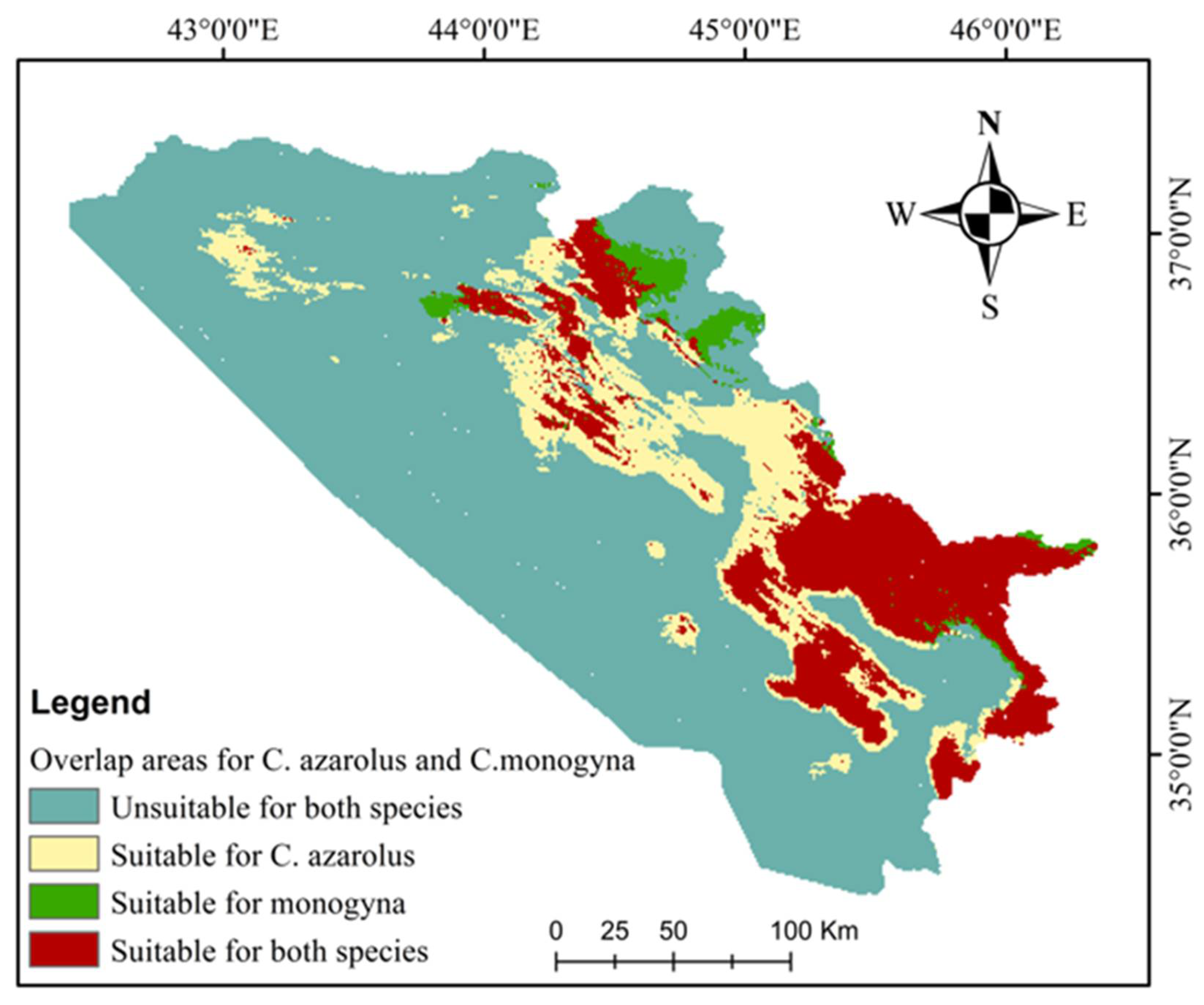
| Class | Area | % |
|---|---|---|
| Unsuitable for both species | 37,750.15 | 73.27 |
| Suitable for C. azarolus only | 5449.10 | 10.58 |
| Suitable for C. monogyna only | 695.02 | 1.35 |
| Suitable for both species | 7626.53 | 14.80 |
| Total area | 51,520.80 | 100.00 |
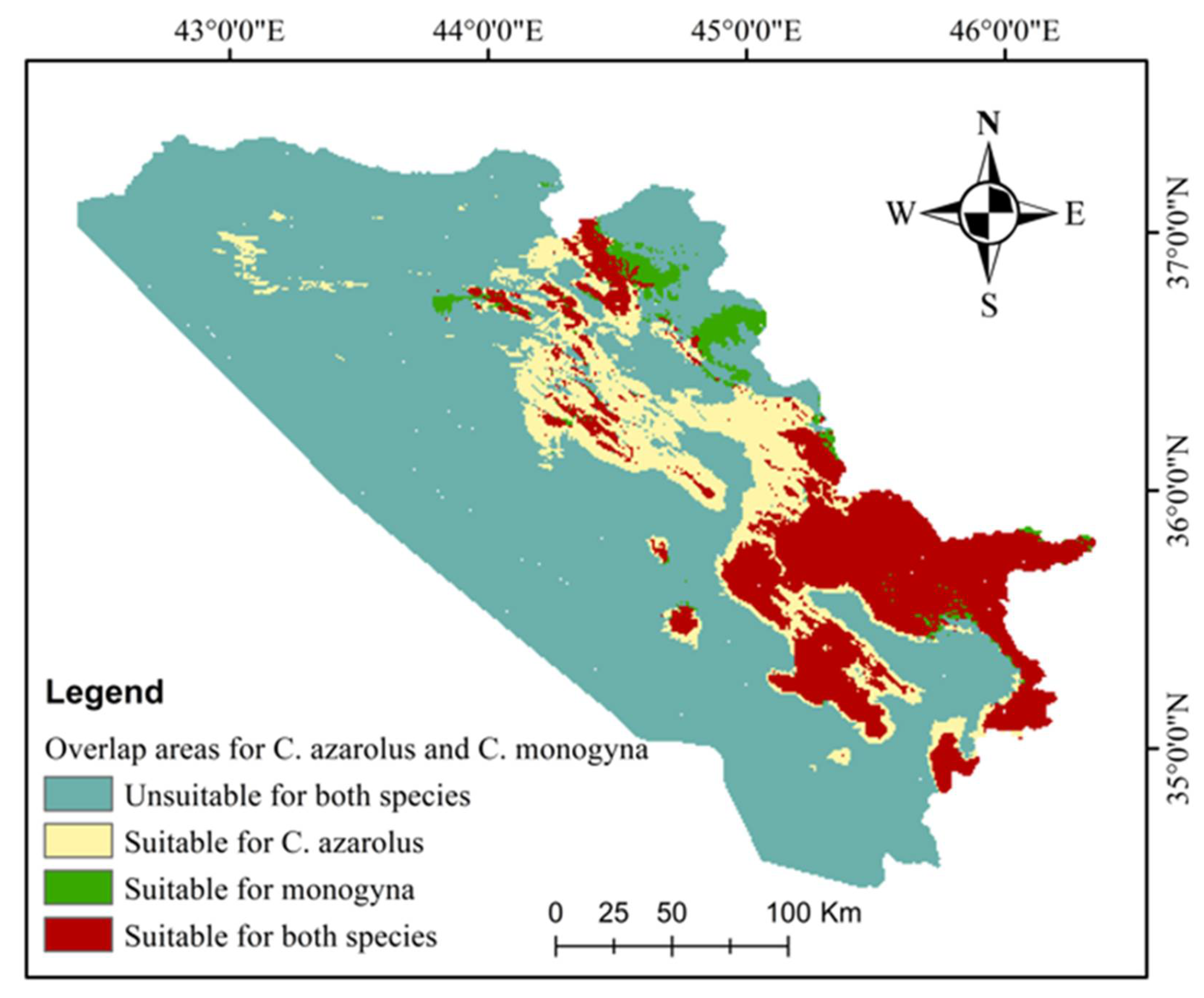
| Class | Area | % |
|---|---|---|
| Unsuitable for both species | 38,147.63 | 74.04 |
| Suitable for C. azarolus only | 5283.82 | 10.26 |
| Suitable for C. monogyna only | 737.90 | 1.43 |
| Suitable for both species | 7351.45 | 14.27 |
| Total area | 51,520.80 | 100.00 |
Publisher’s Note: MDPI stays neutral with regard to jurisdictional claims in published maps and institutional affiliations. |
© 2022 by the authors. Licensee MDPI, Basel, Switzerland. This article is an open access article distributed under the terms and conditions of the Creative Commons Attribution (CC BY) license (https://creativecommons.org/licenses/by/4.0/).
Share and Cite
Radha, K.O.; Khwarahm, N.R. An Integrated Approach to Map the Impact of Climate Change on the Distributions of Crataegus azarolus and Crataegus monogyna in Kurdistan Region, Iraq. Sustainability 2022, 14, 14621. https://doi.org/10.3390/su142114621
Radha KO, Khwarahm NR. An Integrated Approach to Map the Impact of Climate Change on the Distributions of Crataegus azarolus and Crataegus monogyna in Kurdistan Region, Iraq. Sustainability. 2022; 14(21):14621. https://doi.org/10.3390/su142114621
Chicago/Turabian StyleRadha, Kalthum O., and Nabaz R. Khwarahm. 2022. "An Integrated Approach to Map the Impact of Climate Change on the Distributions of Crataegus azarolus and Crataegus monogyna in Kurdistan Region, Iraq" Sustainability 14, no. 21: 14621. https://doi.org/10.3390/su142114621
APA StyleRadha, K. O., & Khwarahm, N. R. (2022). An Integrated Approach to Map the Impact of Climate Change on the Distributions of Crataegus azarolus and Crataegus monogyna in Kurdistan Region, Iraq. Sustainability, 14(21), 14621. https://doi.org/10.3390/su142114621