3.1. Data and Variables
For the purpose of this study, annual data for Croatia, Albania, and the European Union (EU27) covering the period 1995–2024 are used in the analysis. The baseline data for the core analysis were obtained from the World Bank World Development Indicators (WDI) database. The WDI series is retained as the baseline because it provides a harmonized source for Croatia, Albania, and the EU27 over the full study period, while the EEA inventory series is used as an alternative specification to assess source sensitivity. The starting year was selected primarily to avoid war-related disruptions and the strongest early-transition distortions, particularly in Croatia, while providing a sufficiently long and comparable period for the two countries.
Three variables are included in the core analysis: real gross domestic product (GDP), total CO
2 emissions, and carbon intensity. Real GDP is expressed in constant 2015 US dollars (
World Bank, 2026b) and is used to measure economic activity independently of price changes. CO
2 emissions are expressed in million tons of CO
2 equivalent (Mt CO
2e) (
World Bank, 2026a) and refer to total carbon dioxide emissions excluding land use, land use change, and forestry (LULUCF). Carbon intensity is calculated as the ratio of CO
2 emissions to real GDP.
For the alternative-source robustness check, CO
2 emissions data were additionally obtained from the European Environment Agency (EEA) Greenhouse Gases Data Viewer (
EEA, 2026). The EEA series corresponds to the “Total emissions (UNFCCC)” CO
2 category, excluding LULUCF, and covers the same 1995–2024 period. These data are used only as an alternative emissions specification; the World Bank real GDP series is retained throughout the robustness analysis. For the supplementary consumption-based robustness check, Croatia’s CO
2 emission footprint was obtained from Eurostat’s FIGARO carbon dioxide emission footprints dataset (env_ac_co2fp). The series attributes CO
2 emissions along global production chains to final demand and, using the aggregate for all NACE activities plus households, is available for the 2010–2023 period used in this check (
Eurostat, 2026a). The consumption-based robustness check is restricted to Croatia because a comparable consumption-based CO
2 emissions series is not available for Albania in the FIGARO dataset.
For the supplementary LMDI decomposition, total energy supply (TES) was obtained from Eurostat energy balances and is measured in thousand tons of oil equivalent (ktoe) (
Eurostat, 2026c). Energy sector CO
2 emissions were obtained from the EEA Greenhouse Gases Data Viewer using the IPCC Sector 1 (Energy) CO
2 series for Croatia, Albania, and the EU27 (
EEA, 2026). The decomposition covers the same 1995–2024 period. The use of Sector 1 emissions in this supplementary analysis provides a closer correspondence between the emissions measure and the energy variable used in the decomposition.
The EU27 series represents the current membership composition retrospectively over the full period, with the United Kingdom excluded throughout. Croatia is therefore included in the EU27 aggregate throughout the series, although its weight in the aggregate is small. This should be kept in mind when interpreting comparisons between the two national economies and the EU27 benchmark.
Total GDP and total CO2 emissions are used rather than per capita measures because the study focuses on economy-wide decoupling between aggregate economic activity and total territorial emissions. Per capita indicators would address a related but different question by incorporating population dynamics and are therefore outside the scope of the present analysis.
Carbon intensity is calculated as:
where
CIt represents carbon intensity in year t,
CO2,t represents total CO
2 emissions, and
GDPt represents real GDP. A decline in carbon intensity means that less CO
2 is emitted per unit of economic output. It therefore indicates an improvement in the emission efficiency of the economy but not necessarily absolute decoupling, since total emissions may still increase when GDP grows more rapidly.
For the supplementary analysis of regulatory transition exposure, bilateral trade data were obtained from Eurostat Comext (dataset DS-059322, EU trade since 2002 by HS2-4-6 and CN8) for the period 2015–2024 (
Eurostat, 2026b). The EU27 was specified as the reporting area, Albania as the partner country, and imports as the trade flow, with trade values expressed in euros. Both the numerator and denominator of the exposure measure were therefore constructed from the same reporting perspective and data source.
3.2. Analytical Approach
The empirical analysis combines long-term trend assessment with annual and medium-term measures of decoupling. Long-term changes in carbon intensity are first examined using indexed trends and non-parametric trend methods. The relationship between economic growth and CO
2 emissions is then assessed using the Tapio elasticity framework at annual and medium-term horizons. Statistical comparisons and sensitivity checks are used to examine the robustness of the resulting decoupling patterns. An LMDI decomposition is additionally used to examine the contributions of economic activity, energy intensity, and the carbon intensity of energy to changes in energy sector CO
2 emissions. The supplementary CBAM analysis presented in
Section 3.3 adds a regulatory transition risk perspective for Albania.
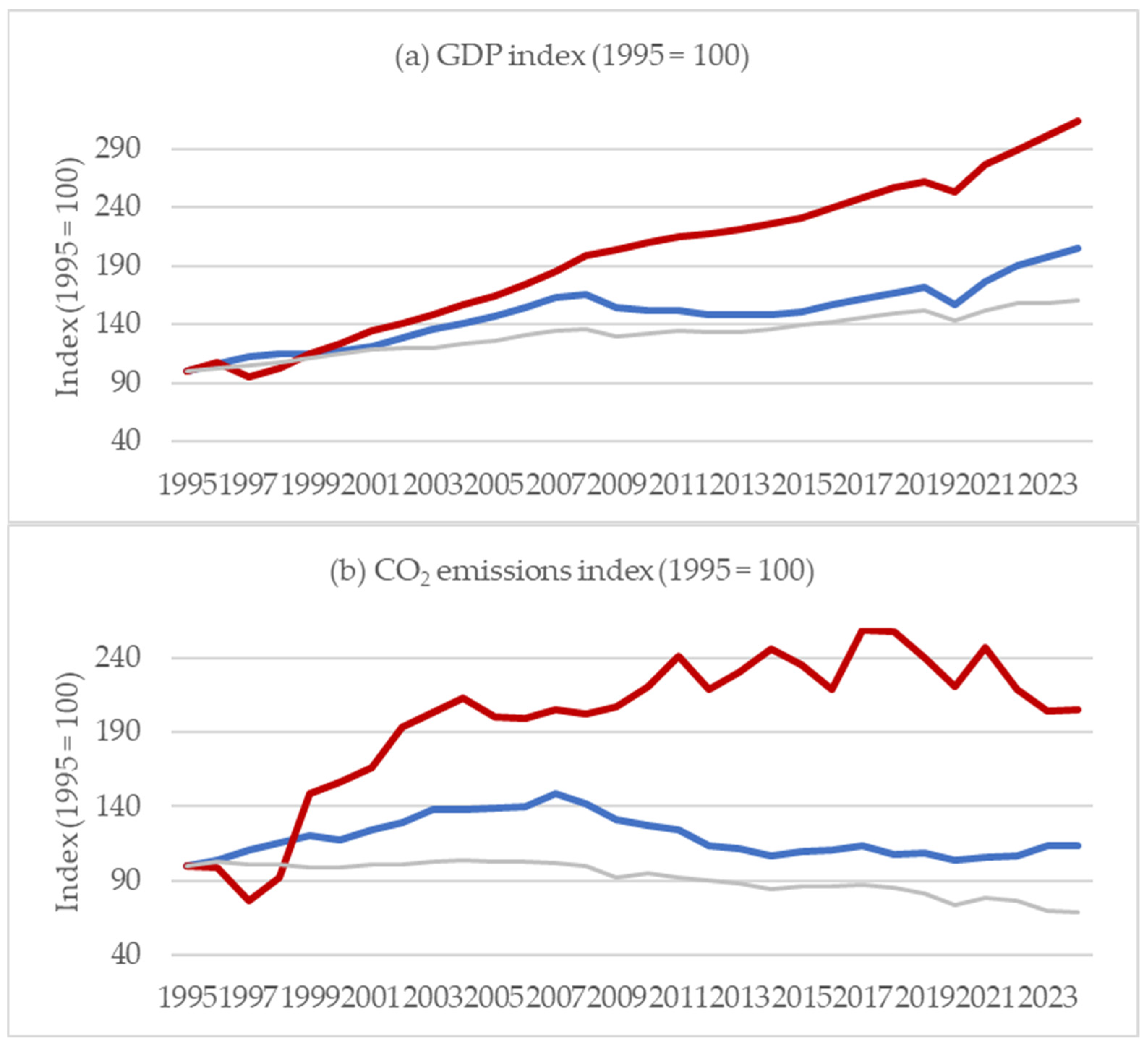
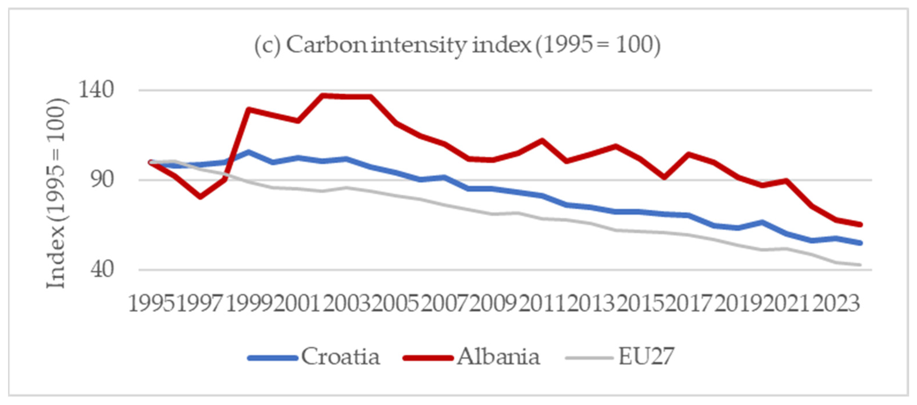
Long-term developments in GDP, CO2 emissions, and carbon intensity are first presented as index series, with 1995 set as the base year (1995 = 100). Indexing allows the relative trajectories of variables measured in different units to be compared across Croatia, Albania, and the EU27 despite substantial differences in their initial levels. This provides a descriptive indication of whether economic growth and emissions have moved together over time or have increasingly diverged.
The long-term trend in carbon intensity is subsequently examined using the Mann–Kendall trend test (
Mann, 1945) and Sen’s slope estimator (
Sen, 1968). The Mann–Kendall test is a non-parametric procedure for detecting monotonic trends and does not require observations to follow a normal distribution. Sen’s slope complements the test by estimating the direction and magnitude of the trend. Statistical significance is assessed at the 5% level.
Because serial autocorrelation can affect inference from the Mann–Kendall test, first-order serial autocorrelation is assessed for each carbon intensity series after detrending. Where significant autocorrelation is detected, the Trend-Free Pre-Whitening (TFPW) procedure of
Yue et al. (
2002) is applied before performing the Mann–Kendall test. The Mann–Kendall test is therefore conducted on the TFPW-adjusted series, while Sen’s slope is estimated from the original time series.
The trend analysis is supplemented by several robustness diagnostics. Lag-1 autocorrelation is reported for each carbon intensity series, and statistical significance is additionally assessed using the Hamed–Rao modified Mann–Kendall test (
Hamed & Rao, 1998), which adjusts the variance of the test statistic for serial dependence. This provides an alternative treatment of autocorrelation and makes it possible to assess whether the inference on the direction and significance of the trend is robust to the method used to address serial dependence. Sen’s slope is also reported with its 95% confidence interval.
Since absolute Sen slopes are affected by differences in carbon intensity levels, the slope is additionally expressed relative to mean carbon intensity:
where
RSi denotes the relative Sen slope for economy
i,
βi is the corresponding Sen slope, and
is mean carbon intensity over the study period. The resulting measure expresses the estimated annual trend as a percentage of the economy’s average carbon intensity level and facilitates comparison across the three economies.
Annual decoupling between changes in real GDP and CO
2 emissions is examined using the Tapio elasticity approach (
Tapio, 2005). Whereas the preceding analysis focuses on longer-term developments in carbon intensity, the Tapio framework captures changes in the relationship between economic activity and emissions from one period to another. The decoupling index is calculated as:
where
DIt denotes the decoupling index in year
t, while
and
denote the annual percentage changes in CO
2 emissions and real GDP, respectively.
The interpretation of the index depends on both its value and the direction of change in GDP and emissions. The same elasticity value may therefore correspond to a different decoupling state depending on whether the economy is expanding or contracting. Following
Tapio (
2005), observations are classified into eight decoupling states using the conventional threshold values of 0.8 and 1.2, as shown in
Table 1. Because annual changes require a preceding-year observation, the annual analysis comprises 29 observations for each economy, covering 1996–2024.
Strong decoupling represents the most favorable state, as real GDP increases while absolute CO2 emissions decline. Weak decoupling also represents a favorable outcome, although emissions continue to increase at a slower rate than GDP. For the comparative frequency analysis, strong and weak decoupling are therefore grouped as favorable decoupling outcomes. The remaining categories distinguish between different forms of coupling and negative decoupling during periods of economic expansion or contraction. This distinction is relevant over a period that includes recessions and major external shocks, since a decline in emissions during an economic contraction does not carry the same interpretation as declining emissions alongside economic growth.
The annual analysis reports the frequency and share of each Tapio state for Croatia, Albania, and the EU27. Favorable annual shares are compared using pairwise two-proportion tests, supplemented by an omnibus chi-square test of differences across the three economies. These tests are used to distinguish descriptive differences in annual frequencies from statistically supported differences in proportions.
The annual analysis is then extended to a medium-term horizon. Changes in GDP and CO2 emissions are calculated over six contiguous endpoint intervals: 1995–2000, 2000–2005, 2005–2010, 2010–2015, 2015–2020, and 2020–2024. For each interval, the percentage change in CO2 emissions is related to the percentage change in real GDP and classified according to the same eight Tapio states used in the annual analysis. The final interval covers four rather than five years because 2024 is the last year in the dataset. These intervals are used as a descriptive medium-term diagnostic rather than as a formal test of persistence.
To reduce dependence on a small number of fixed endpoints, the medium-term analysis is supplemented with rolling five-year windows. The rolling specification covers 25 overlapping intervals, from 1995–2000 to 2019–2024, with the observation window moving forward by one year at a time. This provides a broader view of whether the decoupling pattern remains similar when the timing of the five-year period changes. However, adjacent rolling windows share four years of observations and are therefore not statistically independent. For this reason, the frequency of favorable outcomes across the rolling windows is treated as a descriptive measure of temporal consistency rather than used for inferential comparisons of proportions. The rolling-window analysis is thus intended to assess the medium-term stability of the observed decoupling patterns rather than to provide a formal statistical test of persistence.
The robustness of the Tapio classifications is examined in two additional ways. First, the conventional 0.8/1.2 thresholds are compared with narrower 0.9/1.1 and wider 0.7/1.3 specifications. The alternative thresholds are applied to both the annual observations and the rolling five-year windows. This makes it possible to assess whether the comparative pattern of favorable decoupling depends materially on the conventional boundary values used to distinguish the Tapio states.
Second, particular attention is given to observations in which the change in GDP is close to zero. Since GDP growth appears in the denominator of the Tapio elasticity, very small changes in GDP can generate large elasticity values and potentially unstable classifications. Observations for which |ΔGDP| < 0.5% are therefore identified in both the annual and rolling analyses. Favorable decoupling shares are recalculated after excluding these observations and compared with the baseline results. The observations are retained in the main analysis; their exclusion serves only as a sensitivity check on whether near-zero GDP changes materially affect the comparative findings.
Taken together, the different analytical components capture related but distinct aspects of the growth–emissions relationship. The carbon intensity analysis identifies the direction and rate of long-term change, while the annual Tapio classifications show how frequently favorable decoupling occurs from year to year. The contiguous and rolling analyses provide a medium-term perspective on the stability of these patterns, and the sensitivity checks indicate how strongly the classifications depend on threshold choice and near-zero GDP changes. This distinction is important because a relatively high frequency of favorable annual outcomes does not necessarily imply that decoupling is equally stable across longer time horizons.
Finally, source sensitivity is assessed by repeating the main analysis using the alternative EEA CO
2 series described in
Section 3.1 while retaining the World Bank real GDP series. Carbon intensity trends, annual Tapio classifications, rolling five-year windows, and contiguous medium-term intervals are recalculated for Croatia, Albania, and the EU27.
As a supplementary robustness check, production-based and consumption-based CO2 outcomes were compared for Croatia over their common 2010–2023 period. Consumption-based emissions were used to assess whether the decoupling results are sensitive to emissions embodied in international trade. Using the same real GDP series, carbon intensity changes and annual Tapio classifications were recalculated with the consumption-based CO2 series and compared with the corresponding production-based results.
To provide a more direct decomposition of the factors associated with changes in energy-related CO
2 emissions, an additive Logarithmic Mean Divisia Index (LMDI-I) decomposition based on the Kaya identity was applied following
Ang (
2005). The additive LMDI-I formulation provides an exact decomposition without a residual term (
Ang, 2005). Energy sector CO
2 emissions were expressed as the product of real GDP, energy intensity, and the carbon intensity of energy:
where
TES denotes total energy supply. The change in energy sector CO
2 emissions was decomposed into three additive components: an activity effect, reflecting changes in real GDP; an energy intensity effect, reflecting changes in TES per unit of GDP; and a carbon-intensity-of-energy effect, reflecting changes in energy sector CO
2 emissions per unit of TES.
The decomposition covers 1995–2024 for Croatia, Albania, and the EU27 using the GDP, TES, and energy sector CO
2 series described in
Section 3.1. The main decomposition compares the 1995 and 2024 endpoints, while annual decompositions are used as a supplementary diagnostic of changes over time.
3.3. CBAM Trade Exposure Analysis
To complement the decoupling analysis with a regulatory transition risk perspective, a descriptive CBAM trade exposure indicator is constructed for Albania. The analysis is restricted to Albania because, unlike Croatia, it is a non-EU trading partner whose exports to the EU fall within the external scope of the mechanism, whereas Croatia, as an EU Member State, operates within the EU’s internal carbon-pricing framework. The indicator measures the share of annual EU27 imports from Albania that falls within the product scope of the Carbon Border Adjustment Mechanism (CBAM). For each year
t, CBAM trade exposure is calculated as:
where
CBAM-covered importst denotes the value of EU27 imports from Albania falling within the product scope of Annex I to Regulation (EU) 2023/956, and
Total EU27 imports from Albaniat denotes the total value of EU27 imports from Albania in the same year.
Product coverage is operationalized using the Combined Nomenclature (CN) codes specified in Annex I to Regulation (EU) 2023/956. The relevant codes are assigned to the six CBAM sectors covered by the Regulation: cement, electricity, fertilizers, iron and steel, aluminum, and hydrogen. Where an Annex I heading contains an explicit exclusion, the corresponding non-covered products are removed where the available CN classification permits this. In particular, the exclusions specified within Chapter 72 for iron and steel, including ferrous waste and scrap (CN 7204) and the excluded ferro-alloy categories, are removed from the CBAM-covered trade values. The explicit exclusion of CN 3105 60 00 from the fertilizer category is treated in the same way. This procedure avoids including products outside the regulatory scope and reduces the risk of double counting.
In addition to the aggregate exposure ratio, sector-specific exposure shares are calculated by dividing the annual value of imports in each CBAM sector by total EU27 imports from Albania. The sectoral breakdown is used to identify which product groups account for the observed level and changes in overall CBAM trade exposure.
The indicator should not be interpreted as an estimate of Albania’s actual financial burden under CBAM. Such an estimate would require product-level information on embedded emissions, the applicable EU carbon price, and any carbon price effectively paid in the country of origin. The measure used here instead captures the share of Albania’s exports to the EU that falls within product categories directly covered by the CBAM framework. It is therefore interpreted as an indicator of regulatory trade exposure relevant to transition risk assessment rather than as a measure of monetary compliance costs.
A minor product-mapping limitation concerns CN code ex 2507 00 80 in the current CBAM product scope. The “ex” designation means that only part of the corresponding CN8 category is covered, while the historical Comext data used here do not allow the covered subcomponent to be isolated consistently over the full 2015–2024 period. The full CN8 category is therefore retained in the mapping. Given its very small contribution to total CBAM exposure, this limitation is unlikely to materially affect the overall results.