On the Performance of Lagged Momentum and Reversal Strategies Across Daytime and Overnight Sessions in Bitcoin and Ethereum Cryptocurrencies

Abstract

Cryptocurrency markets trade continuously, but their return dynamics need not be uniform over the 24 h cycle. Using hourly Kraken prices from 2016 to 2025, we divide each day into complementary 12 h sessions and evaluate 25 ordered combinations of cash, long, short, momentum, and reversal positions across all 12 non-redundant hourly boundaries. The full-sample selection identifies Reversal/Reversal at an 08:00 UTC daytime start for Bitcoin (BTC) and Long/Reversal at a 05:00 UTC start for Ethereum (ETH). The return mechanisms differ: BTC is associated with conditional reversal in both sessions, whereas ETH combines positive overnight drift with daytime reversal. The selected rules generate higher realized terminal wealth and more favorable drawdown and Sharpe-ratio outcomes than buy-and-hold along the observed full-sample path. These realized differences, however, are not statistically significant in paired bootstrap tests, and Hansen’s Superior Predictive Ability test does not reject the null after accounting for the search over 300 cutoff–strategy combinations. A chronological holdout exercise, in which selection uses only 2016–2020 and evaluation uses 2021–2025, further shows that the ETH rule persists, but the BTC training-selected rule underperforms buy-and-hold. The findings should therefore be interpreted as evidence of asset-specific historical return structure, not as proof of a stable or readily implementable abnormal-profit opportunity. The 0–2 basis-point cost scenarios are illustrative and exclude slippage, market impact, borrowing, and funding costs.

1. Introduction

Cryptocurrency markets operate continuously, but trading conditions vary systematically throughout the day. Market participation, liquidity, and information arrival change as activity moves across regions and time zones. Consequently, a return measured over a complete 24 h period may combine several shorter return processes. This paper examines whether separating the cryptocurrency trading day into paired sessions reveals return predictability that is not visible in daily returns.

The analysis focuses on Bitcoin (BTC) and Ethereum (ETH), the two largest and most actively traded cryptocurrencies. Although both assets trade around the clock, they need not exhibit the same intraday return behavior. A trading rule that is effective for Bitcoin may not work for Ethereum, and a session boundary that is informative for one asset may be uninformative for the other. This paper therefore does not assume that cryptocurrency markets share a universal daytime or nighttime return pattern.

More specifically, this paper proposes four research questions:

1.

Does dividing the 24 h market into paired daytime and nighttime sessions reveal economically meaningful predictability in returns?

2.

Do the selected session boundaries and trading rules differ between Bitcoin and Ethereum?

3.

Does strategy performance arise from an unconditional session return or from a conditional continuation or reversal pattern?

4.

Do the main findings survive trading costs, multiple-testing adjustment, and chronological holdout evaluation?

We study these questions using hourly BTC and ETH prices from 2016 through 2025. Instead of imposing a single day–night boundary, we compare all 12 non-redundant symmetric session partitions and evaluate simple trading rules constructed from lagged price information. We then assess the resulting full-sample choices using transaction-cost and risk measures, paired block-bootstrap inference, a Superior Predictive Ability test covering the full model search, and a chronological 2016–2020 training/2021–2025 holdout exercise. A separate return-source analysis distinguishes persistent appreciation during a particular session from a conditional response to lagged returns.

The results do not support a single nighttime effect that applies uniformly to both cryptocurrencies. Bitcoin’s full-sample optimum is associated primarily with conditional reversal across the two sessions. Ethereum exhibits a different structure, combining a positive nighttime component with daytime reversal. Although both selected specifications produce large realized wealth ratios relative to buy-and-hold, neither difference reaches conventional statistical significance after accounting for sampling uncertainty and model search. Moreover, the chronological holdout preserves the ETH specification but selects a different BTC rule that subsequently underperforms. The evidence therefore supports asset-specific historical predictability while also showing that positive session returns, in-sample strategy rankings, and stable out-of-sample profitability are distinct claims.

This paper’s main contribution is a transparent framework for identifying the timing and source of short-horizon cryptocurrency return predictability while making the consequences of model selection visible. The rules use hourly prices, lagged returns, and basic position choices without proprietary inputs or an estimated forecasting model. The contribution is not a new momentum or reversal concept; it is the joint organization of familiar rules, paired sessions, return-source tests, and model-search adjustments. This design makes the empirical exercise reproducible, but simplicity alone does not guarantee implementability once fees, slippage, shorting constraints, and exchange-specific execution are considered.

The remainder of this paper is organized as follows. Section 2 reviews the related literature. Section 3 describes the data and return construction. Section 4 presents the session definitions, trading rules, selection procedure, performance measures, and inference. Section 5 reports the main empirical results and statistical tests. Section 6 examines subperiod and chronological holdout evidence, implementation limits, and the exploratory ETF extension. Section 7 concludes. Appendix A reports the complete subperiod strategy matrices.

2. Literature Review

Research on cryptocurrency return predictability begins with the fundamental question of how digital assets are priced. Cryptocurrency returns are not fully explained by the factors commonly used for equities, currencies, and commodities (Liu & Tsyvinski, 2021). However, cryptocurrencies share systematic sources of return variation related to the aggregate market, size, momentum, and investor attention (Liu et al., 2022). Their prices are also formed across fragmented trading venues, where price dispersion and limits to arbitrage can persist even for actively traded assets (Makarov & Schoar, 2020). These features suggest that cryptocurrency returns may reflect both common risk exposures and market-specific trading frictions, making the timing of trading activity potentially relevant for expected returns.

The related literature examines whether cryptocurrency markets reflect weak-form efficiency. Early evidence indicates that Bitcoin returns exhibit statistically detectable dependence, although the degree of predictability varies across sample periods (Urquhart, 2016). Subsequent studies provide further evidence that market efficiency evolves rather than remaining constant. Bariviera documents changes in the persistence of Bitcoin returns over time (Bariviera, 2017), while Khuntia and Pattanayak interpret the changing predictability of Bitcoin through the adaptive-market hypothesis (Khuntia & Pattanayak, 2018). Meanwhile, Sensoy similarly finds that informational efficiency varies with both time and sampling frequency by using high-frequency price (Sensoy, 2019). In these cases, the evidence implies that a strategy that is profitable in one market regime or sample period need not perform equally well in another. This consideration is particularly relevant for cryptocurrencies because their investor base, liquidity, market infrastructure, and institutional participation changed substantially during the development of the market.

The present study is also related to research on the allocation of returns across different parts of the trading day. In conventional financial markets, the institutional opening and closing times provide natural boundaries between overnight and intraday returns. These two return components can display markedly different patterns. Lou et al. show that overnight and intraday expected returns can reflect opposing continuation and reversal forces (Lou et al., 2019). Gao et al. further indicate that returns near the beginning of a trading session can predict returns over the remainder of that session (Gao et al., 2018). This literature demonstrates that aggregating all price changes into a single daily return may conceal economically meaningful within-day return dynamics.

Applying the same framework to cryptocurrencies is less straightforward because cryptocurrency exchanges operate continuously. There is no institutionally determined opening or closing price, and consequently, there is no unique economic definition of daytime and nighttime returns. Any division of the 24 h market must instead be treated as an empirical specification. This distinction matters because changing a session boundary changes not only which hourly returns are classified as daytime or nighttime but also the information used to construct a lagged trading signal.

Existing evidence nevertheless shows that cryptocurrency markets exhibit substantial time-of-day variation. Baur et al. document intraday patterns in Bitcoin returns and trading volume across several exchanges and show that these patterns are not uniformly persistent over time (Baur et al., 2019). Wang et al. identify time-of-day periodicity in Bitcoin trading volume and volatility and examine their relationship with activity in conventional stock markets (Wang et al., 2020). These findings indicate that continuous trading does not imply that information arrival, liquidity, volatility, or investor participation is uniform over the 24 h cycle. They also suggest that conclusions about a daytime or nighttime return effect may be sensitive to the particular hours assigned to each session.

On the other hand, several literature studies show momentum and reversal in cryptocurrency returns. At the cross-sectional level, Grobys and Sapkota provide evidence of momentum among cryptocurrencies (Grobys & Sapkota, 2019). At shorter horizons, Shen et al. document intraday time-series momentum in Bitcoin and relate its strength to periods of elevated trading volume and volatility (Shen et al., 2022). Wen et al. find that intraday momentum and reversal can coexist across cryptocurrency markets, with their relative importance depending on the return horizon and market conditions (Wen et al., 2022). These results imply that cryptocurrency predictability cannot generally be characterized as purely momentum or purely reversal. Instead, the relevant pattern may depend on the asset, trading horizon, sample period, and definition of the return interval.

The closely related literature translates return predictability into implementable trading strategies. Simple technical trading rules have a long history in empirical finance. For example, Brock et al. examine moving-average and trading-range-breakout rules in equity markets and show that simple transformations of past prices can contain information about subsequent returns (Brock et al., 1992). Cryptocurrency studies apply similar ideas to digital assets. Corbet et al. evaluate moving-average oscillator and trading-range-breakout strategies using high-frequency Bitcoin prices and report their strongest evidence for moving-average rules (Corbet et al., 2019). Grobys et al. test technical trading rules across multiple liquid cryptocurrencies (Grobys et al., 2020), while Detzel et al. show that the ratio of the Bitcoin price to its moving average can forecast subsequent returns both in and out of sample (Detzel et al., 2021). Gerritsen et al. examine several trend-following indicators and find that trading-range-breakout rules can outperform a buy-and-hold benchmark in some market conditions (Gerritsen et al., 2020).

Although these strategies are more transparent than many statistical forecasting models, their implementation generally requires the researcher to select moving-average windows, breakout periods, filter sizes, or trading thresholds. Their performance can therefore depend on parameter choices as well as on the underlying return predictability. Transaction costs are also important because signals generated from high-frequency prices can imply frequent changes in position. Consequently, a statistically predictable return does not necessarily translate into an economically profitable trading strategy after implementation costs.

Other studies employ larger predictor sets and more flexible statistical methods. Huang et al. construct 124 price-based technical indicators and use a classification-tree model to predict Bitcoin returns (Huang et al., 2019). Sebastião and Godinho compare machine-learning models for Bitcoin, Ethereum, and Litecoin under changing market conditions and construct trading strategies from ensembles of model signals (Sebastião & Godinho, 2021). Wei et al. combine machine-learning techniques with narrative sentiment, volatility, and time-varying leverage in forecasting and trading Bitcoin (Wei et al., 2023). More generally, the survey by Fang et al. documents the rapid expansion of cryptocurrency trading research across statistical forecasting, technical analysis, machine learning, portfolio construction, and automated trading systems (Fang et al., 2022).

These methods can incorporate more information and capture nonlinear relationships, but they also require additional data, model training, parameter estimation, variable selection, and validation choices. This creates a trade-off between model flexibility and interpretability. Moreover, when many predictors, parameter values, or trading strategies are evaluated, the best observed result may partly reflect repeated model search rather than stable predictability. The data-snooping literature therefore emphasizes that trading-rule performance should be assessed in the context of the full set of alternatives considered (White, 2000). Economic evaluation should likewise account for transaction costs, risk, drawdowns, and stability across sample periods rather than relying exclusively on the highest in-sample terminal wealth.

Taken together, the literature establishes that cryptocurrency returns can be predictable, that this predictability changes over time, and that both simple technical rules and complex forecasting models can exploit parts of it. However, a narrower question remains less developed: how does the preferred conditional trading rule change when a continuously traded cryptocurrency market is divided into alternative paired sessions? Most existing strategies begin with a predetermined daily horizon, a technical indicator window, or an intraday interval. In a market without an official close, fixing a single session boundary may conceal the extent to which the estimated trading pattern depends on that boundary.

The present study addresses this question by jointly organizing session definitions and trading rules within a deliberately parsimonious framework. We divide each 24 h period into complementary daytime and nighttime sessions and evaluate the 12 symmetric 12 h/12 h partitions. Each session is assigned one of five positions—Cash, Long, Short, Momentum, or Reversal—and their ordered combinations generate twenty-five day-night strategies. The Momentum and Reversal positions depend only on the sign of the corresponding lagged session return. Thus, once the session boundary is specified, every position follows from a direct rule based on observed hourly prices.

The contribution is not the introduction of momentum or reversal as new trading concepts. Rather, this paper places these familiar rules in a common session-based framework, evaluates them jointly across alternative boundaries, and compares their performance for Bitcoin and Ethereum. Unlike moving-average strategies, the proposed rules require neither the selection of a signal-formation horizon nor the calibration of an indicator threshold. Unlike machine-learning approaches, they require no estimated forecasting model, order-book information, network variable, or sentiment measure. The analysis further evaluates transaction costs, risk-adjusted performance, drawdowns, turnover, and stability across the 2016–2020 and 2021–2025 sub-periods. The resulting framework is therefore both practical and transparent: the complete strategy set can be reproduced from hourly prices using basic arithmetic, while the sensitivity of the results to the session boundary, asset, trading cost, and sample period remains directly observable.

3. Data

3.1. Data Source and Sample Construction

We use hourly price data for Bitcoin against the U.S. dollar (BTCUSD) and Ethereum against the U.S. dollar (ETHUSD). The data are obtained from Kraken’s official historical market data archive. The sample begins at 00:00 UTC on 1 January 2016 and ends at 23:00 UTC on 31 December 2025. The ten-year period contains 3652 calendar days and 87,672 hourly price observations for each asset.

The original files contain hourly OHLC (Open, High, Low, and Close) prices and volume information. Our analysis uses the closing price because both session returns and strategy signals are constructed from close-to-close price changes. BTC and ETH are evaluated separately, but they share the same hourly timestamp grid and sample period. We do not combine observations from different exchanges or interpolate prices across missing periods.

All timestamps are converted to Coordinated Universal Time (UTC). UTC provides a fixed reference point and avoids changes caused by daylight-saving time. The recorded UTC time is cross-checked against the Unix timestamp included in each file. The validation procedure identifies no missing hours, duplicate timestamps, timestamp mismatches, or non-positive closing prices.

3.2. Return Construction

Let $P_{\tau }$ denote the closing price of an asset at hourly observation $\tau$. The simple hourly return is

$$r_{\tau }={\displaystyle \frac{P_{\tau }}{P_{\tau -1}}}-1,$$

(1)

and the corresponding hourly log return is

$${\mathcal{l}}_{\tau }=ln\left(P_{\tau }\right)-ln\left(P_{\tau -1}\right).$$

(2)

Simple returns are used to construct the trading strategies and wealth series. Log returns are used in the nighttime-return experiment because they can be added across consecutive hourly intervals.

For the trading date t, session s, and cutoff c, the session return is obtained by compounding all hourly simple returns within that session:

$$R_{t,s}\left(c\right)=\prod _{\tau \in {\mathcal{H}}_{t,s}\left(c\right)}(1+r_{\tau })-1,s\in \{N,D\},$$

(3)

where ${\mathcal{H}}_{t,s}\left(c\right)$ is the set of hourly observations assigned to the nighttime session N or daytime session D. Equivalently, the session log return is

$$L_{t,s}\left(c\right)=\sum _{\tau \in {\mathcal{H}}_{t,s}\left(c\right)}{\mathcal{l}}_{\tau }.$$

(4)

We retain only trading dates containing all 12 hourly observations in both sessions. This produces 3652 complete night-day cycles for BTC and ETH under every symmetric cutoff.

3.3. Daytime and Nighttime Definitions

Cryptocurrency markets do not have official opening and closing times. We therefore use the terms ‘daytime’ and ‘nighttime’ as operational labels for two consecutive trading sessions rather than as references to daylight conditions in a particular geographic market.

Let (h) denote the starting hour of the daytime session, expressed in Coordinated Universal Time (UTC). For trading date (t), the nighttime session begins at hour (h + 12) on the preceding calendar date and ends at hour (h) on date (t). The daytime session then begins at hour (h) on date (t) and ends 12 h later. Each session therefore covers 12 h, and the two sessions together form one complete 24 h trading cycle.

The nighttime return, denoted by $r_t^N\left(h\right)$, is measured between the beginning and end of the nighttime session. The daytime return, denoted by $r_t^D\left(h\right)$, is measured between the beginning and end of the daytime session. The full-day return, denoted by $r_t^{24}\left(h\right)$, spans both sessions. Figure 1 illustrates these return intervals.

4. Methodology

4.1. Session-Level Strategy Rules

We apply five possible position rules to the nighttime and daytime sessions independently: cash, long, short, momentum, and reversal. Let $z_{t,s}^j$ denote the position selected by strategy j for the session s on the trading date t. The five positions are defined as

$$z_{t,s}^j=\left\{\begin{array}{cc}0,\hfill & j=\mathrm{Cash},\hfill \\ 1,\hfill & j=\mathrm{Long},\hfill \\ -1,\hfill & j=\mathrm{Short},\hfill \\ sign\left(R_{t-1,s}\right),\hfill & j=\mathrm{momentum},\hfill \\ -sign\left(R_{t-1,s}\right),\hfill & j=\mathrm{Reversal}.\hfill \end{array}\right.$$

(5)

The cash strategy has no exposure to cryptocurrency. The long strategy means keeping a positive unit position, while the short strategy maintains a negative unit position. The momentum strategy takes a long position after a positive return in the previous realization of the same session and a short position after a negative return, while the reversal strategy takes the opposite position.

The time lag in Equation (5) refers to the previous realization of the same session type. The position of the current nighttime session depends on the preceding nighttime return, while the current daytime position depends on the preceding daytime return. The daytime signal does not use the immediately preceding nighttime return. If the lagged return is exactly zero or undefined, as in the first session of the sample, the position is set to cash. This construction ensures that every position is based only on the information available before the corresponding session begins.

Each nighttime rule is combined with one of the five daytime rules. This yields twenty-five night–day strategy combinations for every asset. The gross return of a position during a session is

$$G_{t,s}^j=z_{t,s}^j{R}_{t,s}.$$

(6)

The set of admissible positions is restricted to $\{-1,0,1\}$, so the strategies do not use leverage.

4.2. Illustrative Bitcoin Strategy Examples

To make the strategy rules more transparent, this part provides a hypothetical Bitcoin example. The presentation follows the table-based organization in Salotra et al. (2026), but the strategies are implemented using the same-session lag specification defined in Equation (5). Each strategy is represented by an ordered pair.

$$(\mathrm{Night}\mathrm{rule},\mathrm{Day}\mathrm{rule}),$$

where Long, Short, and Cash correspond to positions of 1, $-1$, and 0, respectively. The five possible rules for each session generate 25 combinations. Strategy 0, $(\mathrm{Cash},\mathrm{Cash})$, is a zero-exposure benchmark, while Strategies 1–24 are active trading strategies.

The Bitcoin returns reported in the table are hypothetical and are used only to illustrate the construction of the positions and strategy returns. All strategies begin with “Cash” during the initialization period. The initialization returns are then used to determine the first dynamic positions on $t_1$. Then, a Momentum position follows the sign of the preceding return from the same session, while a Reversal position takes the opposite sign. Thus, the nighttime position on t depends on the nighttime return on $t-1$, and the daytime position on t depends on the daytime return on $t-1$. To make the economic implications of these positions more transparent, each strategy is accompanied by an illustrative wealth index. The index is normalized to 100 at the beginning of the initialization period and is updated sequentially after each nighttime and daytime session. Specifically, the wealth index evolves according to

$$W_s=W_{s-1}\left(1+p_s{r}_s\right),$$

(7)

where $W_s$ denotes the wealth index after session s, $r_s$ is the hypothetical Bitcoin return during that session, and $p_s$ denotes the corresponding strategy position. The position variable takes the value 1 for Long, $-1$ for Short, and 0 for Cash. Because every strategy remains in Cash during the initialization period, its wealth index remains at 100 in the first two columns. The reported wealth values are purely illustrative and are not part of the empirical results presented in Section 4.

4.2.1. Single-Session Static Strategies

The first group takes a fixed Long or Short position during one session and remains in Cash during the other. Strategy 0 is included as the no-trade benchmark. This is shown in

Table 1. Hypothetical Bitcoin returns and single-session static strategies’ performance (starting balance USD 100).

#	Strategy Rule	Initialization		${\mathit{t}}_1$		${\mathit{t}}_2$		${\mathit{t}}_3$		${\mathit{t}}_4$
		Night	Day	Night	Day	Night	Day	Night	Day	Night	Day
		$1.00\%$	$-2.00\%$	$2.00\%$	$-1.00\%$	$-3.00\%$	$-2.00\%$	$-1.00\%$	$2.00\%$	$4.00\%$	$1.00\%$
0	(Cash, Cash)	Cash	Cash	Cash	Cash	Cash	Cash	Cash	Cash	Cash	Cash
		100	100	100	100	100	100	100	100	100	100
1	(Long, Cash)	Cash	Cash	Long	Cash	Long	Cash	Long	Cash	Long	Cash
		100	100	102.00	102.00	98.94	98.94	97.95	97.95	101.87	101.87
2	(Short, Cash)	Cash	Cash	Short	Cash	Short	Cash	Short	Cash	Short	Cash
		100	100	98.00	98.00	100.94	100.94	101.95	101.95	97.87	97.87
3	(Cash, Long)	Cash	Cash	Cash	Long	Cash	Long	Cash	Long	Cash	Long
		100	100	100	99.00	99.00	97.02	97.02	98.96	98.96	99.95
4	(Cash, Short)	Cash	Cash	Cash	Short	Cash	Short	Cash	Short	Cash	Short
		100	100	100	101.00	101.00	103.02	103.02	100.96	100.96	99.95

.

4.2.2. Combined Static Strategies

The combined static strategies maintain fixed positions during both the nighttime and daytime sessions. Their positions do not depend on previously observed returns. This is shown in

Table 2. Hypothetical Bitcoin returns and combined static strategies.

#	Strategy Rule	Initialization		${\mathit{t}}_1$		${\mathit{t}}_2$		${\mathit{t}}_3$		${\mathit{t}}_4$
		Night	Day	Night	Day	Night	Day	Night	Day	Night	Day
		$1.00\%$	$-2.00\%$	$2.00\%$	$-1.00\%$	$-3.00\%$	$-2.00\%$	$-1.00\%$	$2.00\%$	$4.00\%$	$1.00\%$
5	(Long, Long)	Cash	Cash	Long	Long	Long	Long	Long	Long	Long	Long
		100	100	102.00	100.98	97.95	95.99	95.03	96.93	100.81	101.82
6	(Short, Short)	Cash	Cash	Short	Short	Short	Short	Short	Short	Short	Short
		100	100	98.00	98.98	101.95	103.99	105.03	102.93	98.81	97.82
7	(Short, Long)	Cash	Cash	Short	Long	Short	Long	Short	Long	Short	Long
		100	100	98.00	97.02	99.93	97.93	98.91	100.89	96.85	97.82
8	(Long, Short)	Cash	Cash	Long	Short	Long	Short	Long	Short	Long	Short
		100	100	102.00	103.02	99.93	101.93	100.91	98.89	102.85	101.82

.

4.2.3. Single-Session Dynamic Strategies

The next group applies either a Momentum or a Reversal rule in one session and remains in Cash in the other. Each dynamic position is determined using the preceding return from the same session. This is shown in

Table 3. Hypothetical Bitcoin returns and single-session dynamic strategies.

#	Strategy Rule	Initialization		${\mathit{t}}_1$		${\mathit{t}}_2$		${\mathit{t}}_3$		${\mathit{t}}_4$
		Night	Day	Night	Day	Night	Day	Night	Day	Night	Day
		$1.00\%$	$-2.00\%$	$2.00\%$	$-1.00\%$	$-3.00\%$	$-2.00\%$	$-1.00\%$	$2.00\%$	$4.00\%$	$1.00\%$
9	(Cash, Momentum)	Cash	Cash	Cash	Short	Cash	Short	Cash	Short	Cash	Long
		100	100	100	101.00	101.00	103.02	103.02	100.96	100.96	101.97
10	(Cash, Reversal)	Cash	Cash	Cash	Long	Cash	Long	Cash	Long	Cash	Short
		100	100	100	99.00	99.00	97.02	97.02	98.96	98.96	97.97
11	(Momentum, Cash)	Cash	Cash	Long	Cash	Long	Cash	Short	Cash	Short	Cash
		100	100	102.00	102.00	98.94	98.94	99.93	99.93	95.93	95.93
12	(Reversal, Cash)	Cash	Cash	Short	Cash	Short	Cash	Long	Cash	Long	Cash
		100	100	98.00	98.00	100.94	100.94	99.93	99.93	103.93	103.93

.

4.2.4. Combined Dynamic Strategies

The combined dynamic strategies apply a Momentum or Reversal rule separately to both sessions. Because the two positions are constructed from different lagged session returns, the nighttime and daytime positions do not necessarily point in the same direction. This is shown in

Table 4. HypotheticalBitcoin returns and combined dynamic strategies.

#	Strategy Rule	Initialization		${\mathit{t}}_1$		${\mathit{t}}_2$		${\mathit{t}}_3$		${\mathit{t}}_4$
		Night	Day	Night	Day	Night	Day	Night	Day	Night	Day
		$1.00\%$	$-2.00\%$	$2.00\%$	$-1.00\%$	$-3.00\%$	$-2.00\%$	$-1.00\%$	$2.00\%$	$4.00\%$	$1.00\%$
13	(Momentum, Momentum)	Cash	Cash	Long	Short	Long	Short	Short	Short	Short	Long
		100	100	102.00	103.02	99.93	101.93	102.95	100.89	96.85	97.82
14	(Momentum, Reversal)	Cash	Cash	Long	Long	Long	Long	Short	Long	Short	Short
		100	100	102.00	100.98	97.95	95.99	96.95	98.89	94.93	93.99
15	(Reversal, Momentum)	Cash	Cash	Short	Short	Short	Short	Long	Short	Long	Long
		100	100	98.00	98.98	101.95	103.99	102.95	100.89	104.93	105.97
16	(Reversal, Reversal)	Cash	Cash	Short	Long	Short	Long	Long	Long	Long	Short
		100	100	98.00	97.02	99.93	97.93	96.95	98.89	102.85	101.82

.

4.2.5. Static Night and Dynamic Day Strategies

This group combines a fixed nighttime position with a dynamic daytime position. The daytime position is determined from the preceding daytime return rather than the nighttime return observed on the same date. This is shown in

Table 5. Hypothetical Bitcoin returns and static night–dynamic day strategies.

#	Strategy Rule	Initialization		${\mathit{t}}_1$		${\mathit{t}}_2$		${\mathit{t}}_3$		${\mathit{t}}_4$
		Night	Day	Night	Day	Night	Day	Night	Day	Night	Day
		$1.00\%$	$-2.00\%$	$2.00\%$	$-1.00\%$	$-3.00\%$	$-2.00\%$	$-1.00\%$	$2.00\%$	$4.00\%$	$1.00\%$
17	(Long, Momentum)	Cash	Cash	Long	Short	Long	Short	Long	Short	Long	Long
		100	100	102	103.02	99.93	101.93	100.91	98.89	102.85	103.87
18	(Long, Reversal)	Cash	Cash	Long	Long	Long	Long	Long	Long	Long	Short
		100	100	102	100.98	97.95	95.99	95.03	96.93	100.81	99.80
19	(Short, Momentum)	Cash	Cash	Short	Short	Short	Short	Short	Short	Short	Long
		100	100	98	98.98	101.95	103.99	105.03	102.93	98.81	99.80
20	(Short, Reversal)	Cash	Cash	Short	Long	Short	Long	Short	Long	Short	Short
		100	100	98	97.02	99.93	97.93	98.91	100.89	96.85	95.89

.

4.2.6. Dynamic Night and Static Day Strategies

The final group combines a dynamic nighttime position with a fixed daytime position. The nighttime position is determined from the preceding nighttime return. This is shown in

Table 6. Hypothetical Bitcoin returns and dynamic night–static day strategies.

#	Strategy Rule	Initialization		${\mathit{t}}_1$		${\mathit{t}}_2$		${\mathit{t}}_3$		${\mathit{t}}_4$
		Night	Day	Night	Day	Night	Day	Night	Day	Night	Day
		$1.00\%$	$-2.00\%$	$2.00\%$	$-1.00\%$	$-3.00\%$	$-2.00\%$	$-1.00\%$	$2.00\%$	$4.00\%$	$1.00\%$
21	(Momentum, Long)	Cash	Cash	Long	Long	Long	Long	Short	Long	Short	Long
		100	100	102	100.98	97.95	95.99	96.95	98.89	94.93	95.88
22	(Reversal, Long)	Cash	Cash	Short	Long	Short	Long	Long	Long	Long	Long
		100	100	98	97.02	99.93	97.93	96.95	98.89	102.85	103.88
23	(Momentum, Short)	Cash	Cash	Long	Short	Long	Short	Short	Short	Short	Short
		100	100	102	103.02	99.93	101.93	102.95	100.89	96.85	95.88
24	(Reversal, Short)	Cash	Cash	Short	Short	Short	Short	Long	Short	Long	Short
		100	100	98	98.98	101.95	103.99	102.95	100.89	104.93	103.88

.

4.2.7. Example Return Computation

The section below is meant to illustrate how to convert positions into strategy returns; consider Strategy 13, $(\mathrm{Momentum},\mathrm{Momentum})$. The initialization nighttime return is positive, while the initialization daytime return is negative. The strategy therefore takes a Long nighttime position and a Short daytime position on $t_1$.

Without transaction costs, the strategy return on date t is

$$R_t^S=\left(1+z_{t,N}^S{R}_t^N\right)\left(1+z_{t,D}^S{R}_t^D\right)-1,$$

(8)

where $z_{t,N}^S$ and $z_{t,D}^S$ denote the nighttime and daytime positions, respectively. For Strategy 13 on $t_1$,

$$R_{t_1}^{\left(13\right)}=\left[1+\left(1\right)\left(0.0200\right)\right]\left[1+(-1)(-0.0100)\right]-1=\left(1.0200\right)\left(1.0100\right)-1=0.0302,$$

(9)

which corresponds to a gross strategy return of $3.02\%$. This is illustrated in

Table 7. Illustrative gross returns for Strategy 13: (Momentum, Momentum).

Date	Position		Returns
	Overnight	Daytime	Overnight	Daytime	24 h
	${\mathit{z}}_{\mathit{t},\mathit{N}}$	${\mathit{z}}_{\mathit{t},\mathit{D}}$	${\mathit{R}}_{\mathit{t}}^{\mathit{N}}$	${\mathit{R}}_{\mathit{t}}^{\mathit{D}}$	${\mathit{R}}_{\mathit{t}}^{\left(13\right)}$
$t_1$	1	$-1$	$2.00\%$	$-1.00\%$	$3.02\%$
$t_2$	1	$-1$	$-3.00\%$	$-2.00\%$	$-1.06\%$
$t_3$	$-1$	$-1$	$-1.00\%$	$2.00\%$	$-1.02\%$
$t_4$	$-1$	1	$4.00\%$	$1.00\%$	$-3.04\%$

.

Applying the same calculation to the remaining dates gives the following returns.

If the strategy begins with an initial portfolio value of $W_0=100$, its value after the four hypothetical trading dates is

$$W_4=100\left(1.0302\right)\left(0.9894\right)\left(0.9898\right)\left(0.9696\right)=97.8213.$$

(10)

The corresponding cumulative gross return is therefore

$${\displaystyle \frac{W_4}{W_0}}-1={\displaystyle \frac{97.8213}{100}}-1=-2.1787\%.$$

(11)

This numerical result is purely illustrative and should not be interpreted as empirical evidence about Bitcoin profitability. Transaction costs are excluded here because their treatment is introduced separately in Section 3.3.

These examples also clarify the timing of the signals used in Equation (5). Each dynamic position is determined before the corresponding session begins and uses only the most recently observed return from the same session type. The strategies use only information available at the time of trading and do not rely on future returns.

4.3. Cutoff Selection Procedure

In conventional financial markets, overnight and intraday returns can be defined using official exchange opening and closing times (Lou et al., 2019). Cryptocurrency markets, however, trade continuously and do not have externally determined session boundaries. This distinction is important because previous studies document systematic time-of-day variation in Bitcoin returns, trading volume, and volatility (Baur et al., 2019; Wang et al., 2020), as well as intraday momentum and reversal predictability in cryptocurrency markets (Wen et al., 2022). We therefore evaluate alternative session boundaries instead of imposing a single cutoff without comparison.

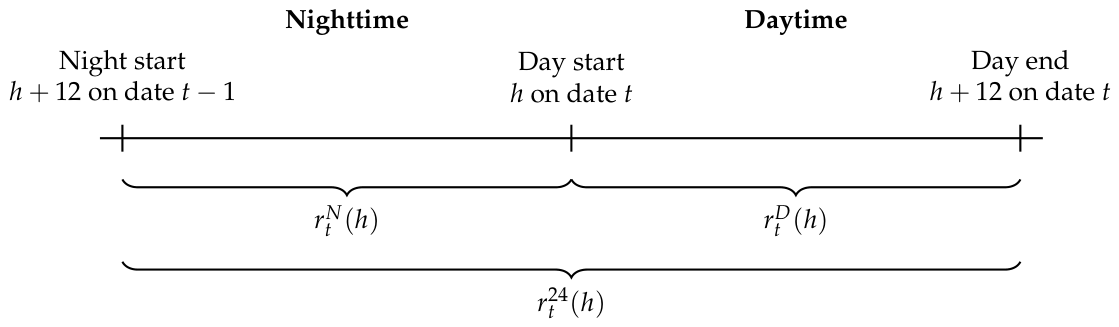
For a candidate daytime starting hour (h), we define the daytime and nighttime sessions as

$$D\left(h\right)=[h,h+12),N\left(h\right)=[h+12,h+24),$$

(12)

where all hours are expressed in UTC and calculated modulo 24. Each specification, therefore, divides the trading day into two non-overlapping 12 h sessions that jointly cover the entire 24 h period.

We consider the following set of candidate daytime starting hours:

$$\mathcal{H}=0,1,\dots ,11.$$

(13)

These 12 specifications represent all non-redundant hourly partitions under the 12 h/12 h restriction. A starting hour of $(h+12)$ produces the same two session boundaries as (h) but reverses the daytime and nighttime labels. Because all ordered combinations of the five session rules are evaluated, testing the remaining 12 starting hours would duplicate the same set of cutoff–strategy outcomes.

For each asset and each candidate cutoff, we rerun all 25 combinations of the Cash, Long, Short, Momentum, and Reversal rules across the two sessions. This produces

$$12\mathrm{cutoffs}\times 25\mathrm{strategies}=300$$

(14)

cutoff–strategy combinations for each cryptocurrency. The Cash/Cash strategy is retained as a normalization check, while the other 24 active strategies are examined in the main performance analysis. All dynamic positions are generated using lagged information so that the position for the current session does not depend on contemporaneous or future returns.

Initial wealth is normalized to 100. Transaction costs are set to zero during the cutoff-selection stage so that the comparison isolates differences attributable to the session boundary and trading rule. Transaction-cost sensitivity is examined separately after the asset-specific cutoffs have been selected.

Let $W_{a,h,s}^{\left(0\right)}$ denote the terminal wealth of the strategy s for asset a, under cutoff h and zero transaction costs. For every candidate cutoff, we first identify the highest terminal wealth among the 25 strategies:

$$W_a^{\ast }\left(h\right)=\underset{s\in \mathcal{S}}{max}{W}_{a,h,s}^{\left(0\right)}.$$

(15)

The asset-specific cutoff and strategy are then selected jointly according to

$$({\widehat{h}}_a,{\widehat{s}}_a)arg\underset{h\in \mathcal{H},,s\in \mathcal{S}}{max}{W}_{a,h,s}^{\left(0\right)}.$$

(16)

This procedure allows the identity of the best-performing strategy to change across cutoff specifications. It therefore captures the interaction between the session boundary and the trading rule rather than evaluating only one predetermined strategy under different cutoffs.

Because both the boundary and the rule are selected by maximizing terminal wealth over the full sample, the selected pair is an in-sample optimum and is mechanically subject to model-selection bias. We therefore treat its terminal wealth as a historical description and evaluate the selection separately with a model-search-adjusted test and a chronological holdout design.

4.4. Transaction Costs and Wealth Accumulation

The baseline results are first calculated without transaction costs. We then repeat the analysis using proportional costs of 1 and 2 basis points per unit of turnover. Let i index the chronological sequence of nighttime and daytime sessions, and let

$$Q_i=|z_i-z_{i-1}|$$

(17)

denote position turnover. Moving from cash to long or short produces turnover of one, while moving directly from long to short produces turnover of two.

For transaction-cost rate c, the net session return is calculated as

$${\tilde{G}}_i=(1+z_i{R}_i)(1-c{Q}_i)-1,c\in \left\{0,1\times {10}^{-4},2\times {10}^{-4}\right\}.$$

(18)

This specification deducts costs (0 bps, 1 bps, or 2 bps) whenever the position changes. These cost levels are sensitivity scenarios rather than a claim about the all-in cost faced by a particular investor. The calculation does not separately model bid–ask spread, price slippage at the session boundary, market impact, exchange-specific fees, short-position borrowing costs, perpetual-futures funding, or taxes. Consequently, the reported net wealth is likely to overstate implementable performance whenever these omitted frictions are material.

All strategies begin with initial wealth of 100. Wealth evolves according to

$$W_i=W_{i-1}(1+{\tilde{G}}_i),W_0=100.$$

(19)

The daily strategy return combines the nighttime and daytime returns assigned to the same trading date:

$$G_t^{\mathrm{daily}}=(1+{\tilde{G}}_{t,N})(1+{\tilde{G}}_{t,D})-1.$$

(20)

4.5. Performance Measures

We compare the 25 strategies using terminal wealth, the annualized Sharpe ratio, maximum drawdown, and turnover. Terminal wealth is

$$W_T=100{\displaystyle \prod _{t=1}^T}(1+G_t^{\mathrm{daily}}).$$

(21)

The Sharpe ratio is calculated from daily net strategy returns. Because the assets trade every day, the ratio is annualized using $\sqrt{365}$:

$$SR=\sqrt{365}{\displaystyle \frac{{\overline{G}}^{\mathrm{daily}}}{\sigma (G^{\mathrm{daily}})}}.$$

(22)

The risk-free rate is set to zero because the analysis focuses on short-horizon cryptocurrency return differences rather than the performance of a funded portfolio.

Maximum drawdown measures the largest decline from a previous wealth peak:

$$MDD=\underset{i}{min}\left({\displaystyle \frac{W_i}{{max}_{j\le i}{W}_j}}-1\right).$$

(23)

We report both the full-sample maximum drawdown and the average annual maximum drawdown. For the annual measure, the wealth index is reset to one at the beginning of each calendar year. The ten-yearly maximum drawdowns from 2016 through 2025 are then averaged. The resulting measure prevents a single drawdown episode from completely determining the risk comparison over the full ten-year sample.

For each asset, cutoff, and transaction-cost assumption, the 25 strategies are ranked by terminal wealth. Sharpe ratios and drawdowns are reported alongside terminal wealth so that the comparison does not depend on ending wealth alone. Since the strategy ranking is conducted using the same sample in which performance is measured, the ranking is interpreted as an in-sample description of session-level predictability.

4.6. Robustness Tests

We conduct four sets of robustness tests. First, we repeat the backtests using transaction costs of 0, 1, and 2 basis points per unit of turnover. This test determines whether the main ranking is driven by frequent position changes.

Second, we divide the ten-year sample into 2016–2020 and 2021–2025. The same strategy definitions are applied to both subperiods. Strategy signals are reset to cash at the first observation of each subperiod, so the evaluation does not use a return from outside the relevant sample. This test shows whether the full-sample results are present in both parts of the sample or concentrated in one period.

Third, we conduct a chronological holdout exercise that separates model selection from evaluation. We use only 2016–2020 to choose the zero-cost terminal-wealth-maximizing cutoff and rule from the complete set of 300 combinations for each asset. The selected specification is then frozen and applied to 2021–2025 under costs of 0, 1, and 2 basis points. No 2021–2025 return enters the selection step. This is a historical holdout rather than a live trading experiment, but it provides a stricter stability check than applying the full-sample selection retrospectively to both subperiods.

Fourth, we conduct a focused cutoff retest. For BTC, the evening boundary is held at 20:00 UTC; for ETH, it is held at 17:00 UTC. We then move the morning boundary while keeping the selected strategy rule unchanged. This allows the daytime and nighttime sessions to have different lengths. The purpose is to determine whether performance depends on an exact 12 h/12 h division or remains present under nearby asymmetric session definitions.

4.7. Statistical Inference

We conduct two sets of statistical tests. The first examines whether the conditional return patterns underlying the preferred trading rules are present in the data. The second evaluates whether the preferred strategies perform differently from the corresponding buy-and-hold benchmarks.

Let $r_{a,s,t}$ denote the return of asset a during session s on trading date t, where $s\in \{N,D\}$ denotes the nighttime and daytime sessions, respectively. For a session assigned the Reversal rule, we measure conditional predictability using

$${\mathsf{\Delta }}_{a,s}=\mathbb{E}\left[r_{a,s,t}|r_{a,s,t-1}<0\right]-\mathbb{E}\left[r_{a,s,t}|r_{a,s,t-1}>0\right].$$

(24)

Under a reversal pattern, the current session return should be higher following a negative lagged same-session return than following a positive lagged same-session return. Accordingly, a positive value of ${\mathsf{\Delta }}_{a,s}$ supports the Reversal rule. We test the null hypothesis $H_0:{\mathsf{\Delta }}_{a,s}=0$ for both Bitcoin sessions and for the Ethereum daytime session. Observations for which the lagged same-session return equals zero are excluded from the positive-versus-negative conditional comparison.

The preferred Ethereum specification assigns the Long rule to the nighttime session. Its statistical basis is therefore evaluated using the unconditional mean nighttime return,

$${\mu }_{\mathrm{ETH},N}=\mathbb{E}\left[r_{\mathrm{ETH},N,t}\right],$$

(25)

with the null hypothesis $H_0:{\mu }_{\mathrm{ETH},N}=0$. This test distinguishes an unconditional nighttime return premium from the conditional reversal effect examined in Equation (24).

We next compare each asset-specific preferred strategy with the corresponding buy-and-hold benchmark. Let $g_{a,t}^P\left(c\right)$ denote the daily net return of the preferred strategy for asset a under a transaction cost of c basis points, and let $g_{a,t}^{BH}$ denote the daily buy-and-hold return. The daily performance differential is defined as

$$d_{a,t}\left(c\right)=ln\left(1+g_{a,t}^P\left(c\right)\right)-ln\left(1+g_{a,t}^{BH}\right).$$

(26)

The use of log-return differences connects the statistical test directly to terminal wealth because

$${\displaystyle \sum _{t=1}^T}{d}_{a,t}\left(c\right)=ln\left({\displaystyle \frac{W_{a,T}^P\left(c\right)}{W_{a,T}^{BH}}}\right).$$

(27)

We test the null hypothesis $H_0:\mathbb{E}\left[d_{a,t}\left(c\right)\right]=0$ at transaction costs of 0, 1, and 2 basis points. A positive mean differential indicates that the preferred strategy generates a higher average log wealth increment than buy-and-hold. Strategy and buy-and-hold returns are paired by trading date throughout the analysis.

Statistical uncertainty is evaluated using the stationary block bootstrap (Politis & Romano, 1994). We use 5000 bootstrap replications and an expected block length of seven calendar days. Resampling consecutive dates preserves short-run dependence in cryptocurrency returns while retaining the pairing between strategy and benchmark returns. We report two-sided bootstrap p-values and 95% percentile confidence intervals. Raw p-values and Holm-adjusted p-values are reported within each asset, sample period, and test family. The tests are conducted for the full 2016–2025 sample and separately for 2016–2020 and 2021–2025.

To account directly for the joint search over session boundaries and trading rules, we additionally apply Hansen’s Superior Predictive Ability (SPA) test (Hansen, 2005). For each asset and transaction-cost level, the candidate universe contains all 300 combinations formed by 12 cutoffs and 25 ordered strategies; Cash/Cash is removed automatically from the studentized statistic because its differential has zero variance. The benchmark is the corresponding buy-and-hold return, performance is measured by the daily log-return differential, and dependence is preserved with 5000 stationary-bootstrap replications and an expected block length of seven days. We report Hansen’s consistent SPA p-value. The null is that no candidate in the searched universe has superior expected performance relative to buy-and-hold.

5. Main Results

This section first reports the selection of the asset-specific day–night cutoffs. It then evaluates terminal wealth under alternative transaction-cost assumptions and compares the risk and risk-adjusted performance of the trading strategies.

5.1. Cutoff Selection Results

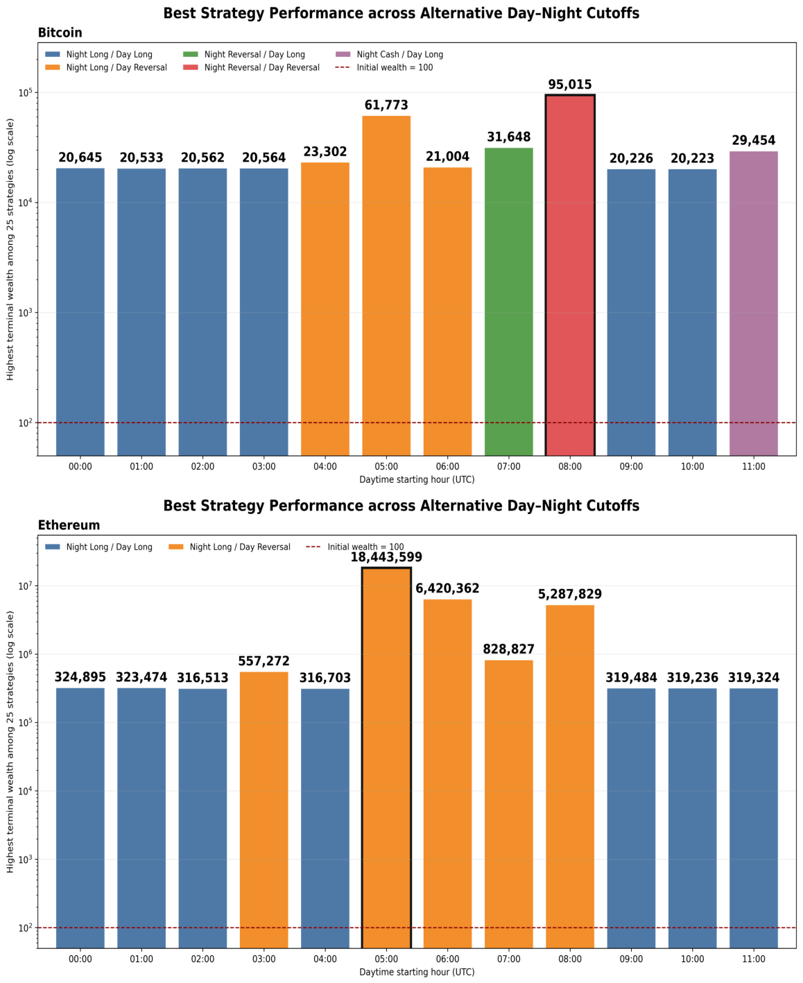
Applying the cutoff-selection procedure described in Section 4.3, we compare the best-performing strategy under each of the 12 alternative day–night partitions. Figure 2 reports the highest terminal wealth among the 25 strategies for each daytime starting hour.

For Bitcoin, the highest terminal wealth is obtained when daytime is defined as 08:00–20:00 UTC and nighttime as 20:00–08:00 UTC. Under this partition, the nighttime Reversal combined with the daytime Reversal strategy produces a terminal wealth of 95,015, the highest value among the 300 Bitcoin cutoff strategy combinations. The corresponding maximum values at the adjacent 07:00 and 09:00 starting hours are 31,648 and 20,226, respectively. The sharp decline on either side of 08:00 is evidence of boundary sensitivity, not a stable economic optimum, and is one reason the selected BTC specification requires holdout validation. In addition, the identity of the best-performing strategy changes across several cutoffs, demonstrating an interaction between the session definition and the trading rule.

For Ethereum, the highest terminal wealth is obtained when daytime is defined as 05:00–17:00 UTC and nighttime as 17:00–05:00 UTC. The nighttime Long combined with the daytime Reversal strategy generates a terminal wealth of 18,443,599 under this specification. The same strategy remains the best-performing rule at the 06:00, 07:00, and 08:00 starting hours, although its terminal wealth is lower than under the 05:00 cutoff. Ethereum’s strongest result, therefore, extends across a broader range of neighboring early-UTC cutoffs, whereas the Bitcoin result is more sharply concentrated around a single starting hour. The two assets exhibit different cutoff–strategy combinations. Bitcoin is characterized by reversal behavior in both sessions under the 08:00 cutoff, whereas Ethereum combines a nighttime long position with a daytime reversal rule under the 05:00 cutoff. This difference suggests that a common session boundary would obscure asset-specific return patterns. Based on these results, the remainder of the analysis uses 08:00–20:00 UTC as the Bitcoin daytime session and 05:00–17:00 UTC as the Ethereum daytime session. These asset-specific cutoffs are held fixed when comparing terminal wealth under alternative transaction costs and when evaluating risk and risk-adjusted performance.

5.2. Terminal Wealth and Transaction-Cost Sensitivity

Table 8. Terminal wealth of Bitcoin and Ethereum strategies, 2016–2025.

#	Strategy		Bitcoin			Ethereum
	Overnight	Daytime	0 bps	1 bp	2 bps	0 bps	1 bp	2 bps
1	Long	Cash	1311	632	304	79,518	38,303	18,449
2	Short	Cash	1	1	0	0	0	0
3	Cash	Long	1542	743	358	402	194	93
4	Cash	Short	0	0	0	0	0	0
5	Long	Long	20,216	20,214	20,212	319,711	319,679	319,647
6	Short	Short	0	0	0	0	0	0
7	Short	Long	19	4	1	0	0	0
8	Long	Short	6	1	0	175	41	9
9	Cash	Momentum	0	0	0	0	0	0
10	Cash	Reversal	3431	1653	796	23,194	11,178	5387
11	Momentum	Cash	1	0	0	3	1	1
12	Reversal	Cash	2770	1334	643	50	24	12
13	Momentum	Momentum	0	0	0	0	0	0
14	Momentum	Reversal	20	10	5	598	292	142
15	Reversal	Momentum	6	3	1	0	0	0
16	Reversal	Reversal	95,015	44,946	21,258	11,652	5550	2644
17	Long	Momentum	3	1	1	3	1	1
18	Long	Reversal	44,978	20,880	9692	18,443,599	8,859,976	4,255,551
19	Short	Momentum	0	0	0	0	0	0
20	Short	Reversal	43	21	11	0	0	0
21	Momentum	Long	9	4	2	10	5	3
22	Reversal	Long	42,706	20,017	9381	202	93	43
23	Momentum	Short	0	0	0	0	0	0
24	Reversal	Short	13	6	3	0	0	0

Notes: Terminal wealth is based on an initial wealth index of 100 and is rounded to the nearest whole unit. Blue-shaded cells denote buy-and-hold. Green-shaded cells exceed the corresponding buy-and-hold value for the same cryptocurrency and transaction cost. Red-shaded cells report remaining strategy outcomes.

reports the terminal wealth of the 24 active strategies for Bitcoin and Ethereum under transaction costs of 0, 1, and 2 basis points. All strategies begin with an initial wealth of 100. The dark-blue cells identify the buy-and-hold benchmark, while the red cells indicate strategies that generate higher terminal wealth than buy-and-hold for the same cryptocurrency and transaction-cost assumption.

For Bitcoin, the strongest result is obtained from Strategy 16, $(\mathrm{Reversal},\mathrm{Reversal})$. With no transaction costs, its terminal wealth reaches 95,015, compared with 20,216 for buy-and-hold. Two other strategies also exceed the benchmark along the realized path in the absence of costs: $(\mathrm{Long},\mathrm{Reversal})$, with a terminal wealth of 44,978, and $(\mathrm{Reversal},\mathrm{Long})$, with a terminal wealth of 42,706. The zero-cost Reversal/Reversal value corresponds to a compound annual growth rate (CAGR) of approximately 98.5%, compared with 70.0% for buy-and-hold. At 2 basis points, the strategy’s realized terminal wealth is only 21,258 versus 20,212 for buy-and-hold, a wealth ratio of 1.05. The paired inference and SPA results below show that these differences are not statistically significant; “above buy-and-hold” here describes the observed sample path, not superior expected performance.

The results for Ethereum are different. Strategy 18, $(\mathrm{Long},\mathrm{Reversal})$, produces the highest terminal wealth under all three transaction-cost assumptions. Its terminal wealth declines from 18,443,599 with no transaction costs to 8,859,976 at 1 basis point and 4,255,551 at 2 basis points. The extreme zero-cost value is generated by repeated compounding over 3652 daily observations and corresponds to a CAGR of approximately 236.2%, compared with 124.1% for buy-and-hold. It should not be interpreted as evidence that capital of arbitrary size could be scaled through the same trades: the calculation omits liquidity-dependent slippage and market impact, and the estimated mean differential remains imprecise. None of the other strategies exceeds Buy-and-hold. The result is therefore not evidence that dynamic trading rules work uniformly for Ethereum. Rather, the realized advantage is concentrated in a specific combination: maintaining a Long position overnight and applying a Reversal rule during the daytime session.

In this case, Table 8 shows that the best-performing rule differs across the two cryptocurrencies. Bitcoin favors a reversal in both sessions, whereas Ether favors a static Long overnight position combined with a daytime reversal. This distinction is consistent with different sources of short-horizon return predictability across the two assets. The table, however, compares strategies only in terms of terminal wealth. Their volatility, maximum drawdown, and risk-adjusted performance are examined separately in the following tables.

5.3. Risk and Risk-Adjusted Performance

Terminal wealth provides a direct measure of the cumulative value generated by each strategy, but it does not fully describe the risk involved in achieving that value. A strategy may produce high terminal wealth while exposing investors to severe peak-to-trough declines, substantial return fluctuations, or an unfavorable trade-off between return and risk. In this case, the terminal-wealth results alone are insufficient to determine whether the dynamic strategies offer a meaningful improvement over buy-and-hold. A more complete evaluation requires examining both downside risk and the stability of strategy returns over the sample period.

Table 9. Risk metrics of Bitcoin and Ethereum strategies, 2016–2025 (0 bps).

#	Strategy		Bitcoin			Ethereum
	Overnight	Daytime	MDD (%)	Sharpe	Vol. (%)	MDD (%)	Sharpe	Vol. (%)
1	Long	Cash	$-70.0$	0.8	42.5	$-84.0$	1.3	65.6
2	Short	Cash	$-99.0$	$-0.8$	42.5	$-100.0$	$-1.3$	65.6
3	Cash	Long	$-70.4$	0.8	51.1	$-85.6$	0.5	68.5
4	Cash	Short	$-99.7$	$-0.8$	51.1	$-99.9$	$-0.5$	68.5
5	Long	Long	$-83.6$	1.1	67.2	$-94.0$	1.3	95.3
6	Short	Short	$-100.0$	$-1.1$	67.3	$-100.0$	$-1.3$	94.8
7	Short	Long	$-87.6$	0.1	66.0	$-100.0$	$-0.5$	94.9
8	Long	Short	$-97.3$	$-0.1$	65.5	$-99.7$	0.5	94.6
9	Cash	Momentum	$-99.9$	$-0.9$	51.1	$-100.0$	$-1.1$	68.4
10	Cash	Reversal	$-55.3$	0.9	51.1	$-92.1$	1.1	68.4
11	Momentum	Cash	$-99.7$	$-1.0$	42.5	$-99.7$	$-0.2$	65.7
12	Reversal	Cash	$-59.3$	1.0	42.5	$-92.4$	0.2	65.7
13	Momentum	Momentum	$-100.0$	$-1.3$	67.3	$-100.0$	$-1.1$	91.3
14	Momentum	Reversal	$-91.4$	0.1	65.8	$-99.2$	0.7	99.2
15	Reversal	Momentum	$-96.6$	$-0.1$	65.3	$-100.0$	$-0.6$	97.5
16	Reversal	Reversal	$-75.1$	1.4	67.5	$-96.1$	1.0	91.5
17	Long	Momentum	$-99.5$	$-0.2$	68.5	$-100.0$	0.1	94.9
18	Long	Reversal	$-79.0$	1.3	64.1	$-73.0$	1.7	94.9
19	Short	Momentum	$-100.0$	$-1.3$	64.1	$-100.0$	$-1.8$	93.8
20	Short	Reversal	$-92.3$	0.2	69.1	$-100.0$	$-0.1$	95.7
21	Momentum	Long	$-98.6$	0.0	67.1	$-99.8$	0.2	97.4
22	Reversal	Long	$-53.5$	1.2	66.0	$-96.8$	0.5	93.0
23	Momentum	Short	$-100.0$	$-1.3$	66.0	$-100.0$	$-0.6$	93.4
24	Reversal	Short	$-97.9$	0.0	66.8	$-99.9$	$-0.2$	96.2

Notes: All figures are computed at 0 bps transaction cost over the full 2016–2025 sample. BTC uses the 8–8–8 UTC session split (day 08:00–20:00; night 20:00–08:00); ETH uses the 5–5–5 UTC session split (day 05:00–17:00; night 17:00–05:00). MDD is the maximum drawdown of the wealth index over the entire ten-year period. The Sharpe ratio is the mean divided by the standard deviation of daily net returns, annualized by $\sqrt{365}$ with a zero risk-free rate. Volatility is the annualized standard deviation of daily net returns. Blue-shaded cells denote buy-and-hold (Long overnight/Long daytime). Green-shaded cells are superior to the corresponding buy-and-hold metric for the same cryptocurrency: a less negative drawdown, a higher Sharpe ratio, or a lower volatility. Red-shaded cells report remaining strategy outcomes.

reports three complementary risk measures with zero transaction costs: maximum drawdown (MDD), annualized Sharpe ratio, and annualized volatility. MDD measures the largest peak-to-trough decline and captures the severity of losses that an investor could experience while applying a strategy. Annualized volatility measures the overall variability of returns, while the Sharpe ratio evaluates return relative to that variability. In these cases, these measures help determine whether the strategies that generate higher terminal wealth also provide more favorable risk characteristics. Buy-and-hold is used as the benchmark for each cryptocurrency, and the green-shaded cells indicate strategies that improve on the corresponding benchmark metric.

For Bitcoin, the preferred Reversal/Reversal strategy delivers a substantially higher Sharpe ratio and a shallower maximum drawdown than buy-and-hold, while its annualized volatility remains approximately unchanged. This distinction is important. The strategy does not outperform by broadly suppressing short-term price fluctuations; rather, it improves the return earned per unit of volatility and reduces the severity of cumulative peak-to-trough losses. Applying reversal in both sessions allows the position to respond conditionally to prior same-session returns, rather than maintaining uninterrupted long exposure throughout the market cycle. The resulting performance is therefore not simply compensation for taking greater market risk.

For Ethereum, the preferred Long/Reversal strategy indicates an even broader improvement in the risk profile. Maintaining a long position overnight while applying reversal during the daytime produces a markedly smaller maximum drawdown and a higher Sharpe ratio than buy-and-hold, together with slightly lower annualized volatility. This result highlights the distinct economic roles of the two Ethereum sessions: the strategy preserves overnight market exposure while adjusting daytime exposure based on the reversal signal. Its terminal-wealth advantage is therefore accompanied by meaningful downside risk protection rather than being generated by additional volatility.

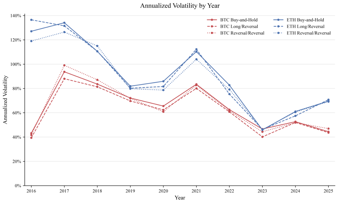
The full-sample risk measures reported above summarize volatility over the entire sample period, but they do not show how the risk of each strategy changes across market conditions. To examine this temporal variation, Figure 3 reports annualized volatility separately for each calendar year. In addition to buy-and-hold, the figure includes the Long/Reversal and Reversal/Reversal strategies for both BTC and ETH. This broader comparison allows the volatility profile of each preferred strategy to be evaluated against both passive exposure and an alternative conditional trading rule.

Figure 3 reveals substantial time variation in cryptocurrency risk.

As shown in Figure 3, volatility was relatively high during 2017–2018 and increased again in 2021, before declining sharply in 2022 and reaching its lowest level in 2023. Volatility subsequently increased for both assets in 2024. In 2025, ETH volatility remained elevated relative to 2023, whereas BTC volatility declined slightly. ETH was generally more volatile than BTC throughout the sample, although the difference narrowed considerably in 2023.

Within each asset, the three strategies follow broadly similar volatility cycles and reach their turning points at approximately the same time. This co-movement indicates that market-wide conditions remain the primary source of annual variation in cryptocurrency volatility. The conditional strategies change the magnitude of volatility in individual years, but they do not remove the underlying volatility regimes of the two assets.

For BTC, both conditional strategies produce lower volatility than buy-and-hold in several middle and later years. However, the preferred Reversal/Reversal strategy does not have the lowest volatility in every year and exceeds buy-and-hold volatility in periods such as 2017, 2018, and 2025. For ETH, the preferred Long/Reversal strategy produces lower volatility than buy-and-hold in most years after 2018, although this reduction is not uniform across the sample. The Reversal/Reversal strategy also reduces ETH volatility in several periods, but its relative position changes over time.

These results show that there is no specific rule that uniformly minimizes annualized volatility in every calendar year. The preferred strategies are not selected solely because they produce the lowest volatility. Their economic performance must instead be evaluated jointly using terminal wealth, volatility, the Sharpe ratio, and maximum drawdown. The following figure provides this broader comparison of risk-adjusted performance and downside exposure.

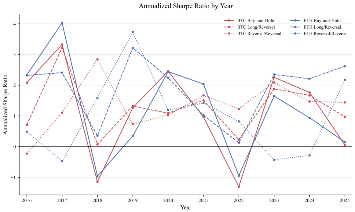
Annualized volatility describes the variability of returns, but it does not show how much return a strategy generates per unit of risk. Figure 4 therefore reports the annualized Sharpe ratio separately for each calendar year. The comparison includes buy-and-hold, Long/Reversal, and Reversal/Reversal for both BTC and ETH, allowing the preferred strategies to be evaluated across different market conditions.

Figure 4 shows that annual risk-adjusted performance varies substantially across time. No strategy produces the highest Sharpe ratio in every calendar year. For BTC, the preferred Reversal/Reversal strategy performs particularly well during years in which buy-and-hold performs poorly. In 2018 and 2022, BTC buy-and-hold records a negative Sharpe ratio, whereas Reversal/Reversal remains positive. Reversal/Reversal also produces a higher Sharpe ratio than buy-and-hold in 2021 and 2025. However, buy-and-hold or Long/Reversal performs better during several strong BTC market years. The preferred BTC strategy therefore improves the stability of risk-adjusted performance without dominating every annual comparison.

The results for ETH provide stronger support for the preferred Long/Reversal strategy. Long/Reversal produces a substantially higher Sharpe ratio than ETH buy-and-hold in 2018, 2019, 2022, 2023, 2024, and 2025. Its advantage is especially important in 2018 and 2022, when the Sharpe ratio of ETH buy-and-hold becomes negative, while Long/Reversal remains positive. Nevertheless, buy-and-hold performs better in some earlier years, including 2017, 2020, and 2021. The annual evidence therefore indicates that the ETH Long/Reversal strategy provides a relatively persistent, but not universal, improvement in risk-adjusted performance.

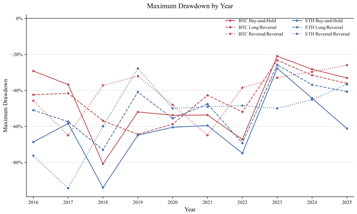
The Sharpe ratio combines returns and volatility, but it does not fully describe the path of cumulative losses. To examine downside exposure directly, Figure 5 reports the maximum drawdown calculated separately within each calendar year. A value closer to zero represents a shallower peak-to-trough decline and therefore stronger downside protection.

Figure 5 shows that the downside-risk advantage of the BTC Reversal/Reversal strategy is concentrated in particular market environments. The strategy produces substantially shallower drawdowns than BTC buy-and-hold in 2018, 2019, and 2022, which are also years in which the Sharpe-ratio comparison favors the reversal rule. It also provides more moderate improvements in several other years. However, Reversal/Reversal generates larger drawdowns than buy-and-hold in some periods, including 2016, 2017, and 2021. Its risk advantage is therefore episodic rather than uniform.

For ETH, the preferred Long/Reversal strategy provides more consistent downside protection. Its annual maximum drawdown is generally less severe than that of ETH buy-and-hold, with particularly visible improvements in 2016, 2018, 2019, 2024, and 2025. The difference is smaller in some years, and Long/Reversal does not outperform buy-and-hold in every annual observation. Nevertheless, the overall pattern indicates that the strategy reduces the severity of ETH drawdowns across a broad range of market conditions.

Taken together, the annual Sharpe-ratio and maximum-drawdown results complement the full-sample risk measures reported above. The BTC Reversal/Reversal strategy provides meaningful protection during several important downturns but does not dominate buy-and-hold in every year. In contrast, the ETH Long/Reversal strategy exhibits a more persistent improvement in both risk-adjusted performance and downside exposure. These findings show that the benefits of the preferred strategies are economically relevant but remain dependent on the prevailing market environment.

5.4. Statistical Evidence on Conditional Predictability and Strategy Performance

We next evaluate the statistical significance of the return mechanisms underlying the preferred trading rules and their performance relative to buy-and-hold. The tests are reported for the full 2016–2025 sample and separately for 2016–2020 and 2021–2025.

Table 10. Conditional predictability under the preferred session definitions: full sample and subperiods.

Asset	Session	Rule	N	Conditional Mean		Estimate	95% CI	Holm p
				Positive Lag	Negative Lag
Panel A: Full Sample, 2016–2025
BTC	Nighttime	Reversal	3651	−1.98	21.92	${23.89}^{ \ast \ast \ast }$	[8.33, 40.16]	0.003
BTC	Daytime	Reversal	3651	−2.08	25.63	${27.71}^{ \ast \ast \ast }$	[11.25, 43.76]	0.002
ETH	Nighttime	Long	3652	–	–	${24.15}^{ \ast \ast \ast }$	[12.60, 36.40]	<$0.001$
ETH	Daytime	Reversal	3651	−10.98	31.80	${42.79}^{ \ast \ast \ast }$	[21.66, 64.85]	<$0.001$
Panel B: 2016–2020
BTC	Nighttime	Reversal	1825	1.63	22.17	${20.54}^{ \ast }$	[−5.01, 46.95]	0.120
BTC	Daytime	Reversal	1825	3.37	37.64	${34.27}^{ \ast \ast }$	[8.95, 58.37]	0.021
ETH	Nighttime	Long	1826	–	–	${40.93}^{ \ast \ast \ast }$	[21.27, 62.24]	0.001
ETH	Daytime	Reversal	1825	−7.83	32.15	${39.98}^{ \ast \ast }$	[5.93, 73.99]	0.020
Panel C: 2021–2025
BTC	Nighttime	Reversal	1825	−5.61	21.66	${27.27}^{ \ast \ast }$	[8.46, 48.23]	0.013
BTC	Daytime	Reversal	1825	−8.00	14.72	${22.72}^{ \ast \ast }$	[2.59, 42.98]	0.030
ETH	Nighttime	Long	1826	–	–	${7.37}^{ \ast }$	[−5.52, 19.86]	0.259
ETH	Daytime	Reversal	1825	−14.10	31.58	${45.68}^{ \ast \ast \ast }$	[19.68, 71.97]	0.003

Notes: Returns and estimates are expressed in basis points per session. For a Reversal rule, Positive Lag and Negative Lag report the mean current-session return conditional on the sign of the lagged same-session return. The estimate is the negative-lag mean minus the positive-lag mean. For the ETH nighttime Long rule, the estimate is the unconditional mean nighttime return. Confidence intervals are 95% percentile intervals from 5000 stationary-block-bootstrap replications with an expected block length of seven calendar days. Reported p-values are two-sided and Holm-adjusted within each asset, sample period, and test family. ***, **, and * denote significance at the 1%, 5%, and 10% levels, respectively.

reports the conditional-predictability results. For a Reversal rule, the estimate compares the mean current-session return following a negative lagged same-session return with the corresponding mean following a positive lagged same-session return. For the Ethereum nighttime Long rule, the estimate is the unconditional mean nighttime return.

The full-sample results provide strong support for the preferred session-level rules. For Bitcoin, the nighttime reversal contrast is 23.89 basis points per session, with a 95% confidence interval of [8.33, 40.16] and a Holm-adjusted p-value of 0.003. The daytime reversal contrast is 27.71 basis points, with a confidence interval of [11.25, 43.76] and an adjusted p-value of 0.002. Both components of the Bitcoin Reversal/Reversal strategy are therefore supported by the full-sample conditional-return evidence.

Ethereum exhibits a different combination of return mechanisms. The daytime reversal contrast is 42.79 basis points, with a 95% confidence interval of [21.66, 64.85] and an adjusted p-value below 0.001. The unconditional mean nighttime return is 24.15 basis points per session, with a confidence interval of [12.60, 36.40] and an adjusted p-value below 0.001. These findings support the Reversal rule during the Ethereum daytime session and the Long rule during the nighttime session.

The subperiod results reveal meaningful time variation. For Bitcoin, the nighttime reversal contrast is not statistically significant during 2016–2020 but becomes significant during 2021–2025. The daytime reversal contrast remains significant at the 5% level in both subperiods. For Ethereum, daytime reversal is also significant in both periods. In contrast, the positive nighttime mean is strongly significant during 2016–2020 but is no longer significant during 2021–2025. Thus, daytime reversal is more stable across the two subperiods than either Bitcoin nighttime reversal or the unconditional Ethereum nighttime return.

Table 11. Preferred strategies versus buy-and-hold: full sample and subperiods.

Asset	Preferred Strategy	Cost (bps)	N	Performance Relative to Buy-and-Hold
				Mean Log Diff. (bps/day)	Annualized Diff. (%)	95% CI	Holm p	Wealth Ratio
Panel A: Full Sample, 2016–2025
BTC	Reversal/Reversal	0	3652	4.24	15.47	[−13.85, 23.00]	1.000	4.70
BTC	Reversal/Reversal	1	3652	2.19	7.99	[−15.92, 20.94]	1.000	2.22
BTC	Reversal/Reversal	2	3652	0.14	0.50	[−17.99, 18.92]	1.000	1.05
ETH	Long/Reversal	0	3652	11.10	40.53	[−4.80, 26.07]	0.498	57.69
ETH	Long/Reversal	1	3652	9.10	33.20	[−6.87, 24.10]	0.500	27.72
ETH	Long/Reversal	2	3652	7.09	25.87	[−8.90, 22.13]	0.500	13.31
Panel B: 2016–2020
BTC	Reversal/Reversal	0	1826	−5.37	−19.59	[−34.42, 24.18]	1.000	0.38
BTC	Reversal/Reversal	1	1826	−7.38	−26.93	[−36.40, 22.15]	1.000	0.26
BTC	Reversal/Reversal	2	1826	−9.39	−34.28	[−38.42, 20.11]	1.000	0.18
ETH	Long/Reversal	0	1826	7.99	29.15	[−17.24, 32.13]	1.000	4.30
ETH	Long/Reversal	1	1826	5.99	21.86	[−19.32, 30.18]	1.000	2.98
ETH	Long/Reversal	2	1826	3.99	14.57	[−21.37, 28.25]	1.000	2.07
Panel C: 2021–2025
BTC	Reversal/Reversal	0	1826	13.89	50.71	[−7.26, 35.66]	0.609	12.64
BTC	Reversal/Reversal	1	1826	11.81	43.10	[−9.31, 33.56]	0.609	8.64
BTC	Reversal/Reversal	2	1826	9.72	35.48	[−11.37, 31.48]	0.609	5.90
ETH	Long/Reversal	0	1826	14.27	52.08	[−4.55, 33.14]	0.412	13.53
ETH	Long/Reversal	1	1826	12.25	44.71	[−6.60, 31.15]	0.412	9.36
ETH	Long/Reversal	2	1826	10.23	37.35	[−8.65, 29.18]	0.412	6.48

Notes: The mean log difference is $\mathrm{10,000}$ times the sample mean of $ln(1+g_t^P)-ln(1+g_t^{BH})$ and is reported in basis points per day. The annualized difference equals 365 times the mean daily log difference. The wealth ratio is preferred-strategy terminal wealth divided by buy-and-hold terminal wealth. Confidence intervals and two-sided p-values are obtained from 5000 paired stationary-block-bootstrap replications with an expected block length of seven calendar days. Reported p-values are Holm-adjusted across the three transaction-cost specifications within each asset and sample period. Buy-and-hold follows the passive-benchmark convention used elsewhere in this paper.

compares the preferred strategies with their corresponding buy-and-hold benchmarks. The test is based on the paired daily log-return difference between each preferred strategy and buy-and-hold.

In the full sample, the mean daily log-return differential for Bitcoin is 4.24 basis points without transaction costs and declines to 0.14 basis points at a cost of 2 basis points; for Ethereum, the corresponding differential declines from 11.10 to 7.09 basis points. The implied terminal wealth ratios are economically large: 4.70 for Bitcoin and 57.69 for Ethereum at zero cost—yet every 95% confidence interval contains zero, and none of the Holm-adjusted p-values approaches conventional significance levels. Therefore, we fail to reject equality of expected log performance between the preferred strategies and buy-and-hold.

This failure to reject reflects the limited power of the test rather than evidence of equal performance. The differential is a small mean embedded in the difference between two highly volatile return series, and its sample standard deviation is large relative to that mean. At the full-sample point estimates, detecting the Ethereum differential at the 5% level would require on the order of two decades of daily observations, and the Bitcoin differential would require an order of magnitude longer still. The confidence intervals are correspondingly wide: at zero cost, the Bitcoin bounds span annualized differentials of roughly $-51\%$ to $+84\%$ and the Ethereum bounds roughly $-18\%$ to $+95\%$. Estimates this imprecise cannot separate the preferred strategies from the passive benchmark in either direction. The wealth ratios should be read in this light; they are realized values along a single historical path and carry no attached sampling uncertainty.

Transaction costs affect the two assets asymmetrically. Each additional basis point of cost reduces the daily differential by approximately two basis points for both assets, consistent with the two trading legs per day implied by the session-based rules. Because Bitcoin’s gross differential is smaller, this erosion is nearly complete: at a cost of 2 basis points, the strategy’s terminal wealth is only 1.05 times that of buy-and-hold, so essentially the entire gross advantage is consumed by trading frictions. Ethereum’s larger gross differential leaves a substantial margin at the same cost level, with a wealth ratio of 13.31, although the estimate remains statistically indistinguishable from zero.

The relative-performance estimates vary considerably across different sub-periods, and for Bitcoin the variation is a change in sign rather than of magnitude. During 2016–2020 the Reversal/Reversal strategy underperforms buy-and-hold at every cost level, with terminal wealth ratios between 0.38 and 0.18; during 2021–2025 it outperforms, with ratios between 12.64 and 5.90. Ethereum’s Long/Reversal strategy has a positive differential in both sub-periods, although the point estimate nearly doubles between them. None of the strategy-benchmark differences is statistically significant at any transaction-cost level. This instability, together with the deterioration of the Ethereum nighttime premium documented in Table 10, cautions against reading the full-sample estimates as descriptions of a stable relationship.

The two tests address different claims. The conditional-predictability results establish that the lagged session signals contain information about subsequent session returns. The strategy comparison instead asks whether that information translates into a precisely estimated incremental return relative to continuous passive exposure, which is a considerably more demanding standard. The comparison is also conducted on raw log returns, so a rule that is out of the market for a substantial fraction of the sample is measured against a fully invested benchmark without adjustment for the difference in exposure. The evidence supports the economic mechanisms underlying the preferred rules, particularly daytime reversal, but it does not establish statistically significant improvement over buy-and-hold, and we do not interpret the strategies as implementable sources of abnormal return.

Table 12. Hansen superior predictive ability test over the full cutoff–strategy search.

Asset	Cost	Candidates	Best Cutoff	Best Rule	SPA p	Decision
BTC	0 bps	300	08:00	Reversal/Reversal	0.899	Fail to reject
BTC	1 bp	300	08:00	Reversal/Reversal	0.954	Fail to reject
BTC	2 bps	300	08:00	Reversal/Reversal	0.996	Fail to reject
ETH	0 bps	300	05:00	Long/Reversal	0.656	Fail to reject
ETH	1 bp	300	05:00	Long/Reversal	0.707	Fail to reject
ETH	2 bps	300	05:00	Long/Reversal	0.771	Fail to reject

Notes: The table reports Hansen’s consistent SPA p-value for the null that no candidate in the complete search universe has superior expected daily log performance relative to buy-and-hold. The universe contains 12 cutoffs × 25 ordered strategies. Cash/Cash remains in the reported candidate count but is excluded from the studentized statistic because its return differential has zero variance, leaving 299 numerical competitors. Results use 5000 stationary-bootstrap replications with an expected block length of seven days.

strengthens the caution implied by the paired strategy tests. The consistent SPA p-values range from 0.899 to 0.996 for Bitcoin and from 0.656 to 0.771 for Ethereum. We therefore fail to reject the null at every cost level after accounting for the complete search over boundaries and rules. The selected specifications are the realized terminal-wealth maxima, but their rankings do not constitute statistically reliable evidence of superior expected performance once repeated model search is incorporated into inference.

6. Discussion and Future Work

6.1. Sub-Period Stability

We have tested the performance of the two preferred strategies across the 2016–2020 and 2021–2025 sub-periods. The Bitcoin analysis retains the 08:00–20:00 UTC daytime session and the Reversal/Reversal strategy, while the Ethereum analysis retains the 05:00–17:00 UTC daytime session and the Long/Reversal strategy. Appendix

Table A1. Terminal wealth of Bitcoin and Ethereum strategies, 2016–2020.

#	Strategy		Bitcoin			Ethereum
	Overnight	Daytime	0 bps	1 bp	2 bps	0 bps	1 bp	2 bps
1	Long	Cash	490	340	236	44,038	30,564	21,212
2	Short	Cash	7	5	3	0	0	0
3	Cash	Long	1365	948	658	178	123	86
4	Cash	Short	1	1	1	2	2	1
5	Long	Long	6691	6690	6689	78,259	78,251	78,243
6	Short	Short	0	0	0	0	0	0
7	Short	Long	97	47	22	0	0	0
8	Long	Short	7	3	2	957	461	222
9	Cash	Momentum	3	2	1	1	0	0
10	Cash	Reversal	697	484	336	764	530	368
11	Momentum	Cash	10	7	5	2	2	1
12	Reversal	Cash	360	250	174	233	162	113
13	Momentum	Momentum	0	0	0	0	0	0
14	Momentum	Reversal	67	47	32	19	13	9
15	Reversal	Momentum	10	7	5	1	1	1
16	Reversal	Reversal	2511	1739	1204	1783	1235	856
17	Long	Momentum	13	9	7	223	155	107
18	Long	Reversal	3415	2290	1535	336,367	233,566	162,172
19	Short	Momentum	0	0	0	0	0	0
20	Short	Reversal	49	35	25	0	0	0
21	Momentum	Long	131	92	65	4	3	2
22	Reversal	Long	4918	3376	2318	415	281	190
23	Momentum	Short	0	0	0	0	0	0
24	Reversal	Short	5	3	2	5	4	3

Notes: Terminal wealth is based on an initial wealth index of 100 and is rounded to the nearest whole unit. BTC results use the 8–8–8 UTC specification (daytime 08:00–20:00 and overnight 20:00–08:00), whereas ETH results use the 5–5–5 UTC specification (daytime 05:00–17:00 and overnight 17:00–05:00). Blue-shaded cells denote buy-and-hold. Green-shaded cells exceed the corresponding buy-and-hold value for the same cryptocurrency and transaction-cost assumption. Red-shaded cells report the remaining strategy outcomes.

and

Table A2. Terminal wealth of Bitcoin and Ethereum strategies, 2021–2025.

#	Strategy		Bitcoin			Ethereum
	Overnight	Daytime	0 bps	1 bp	2 bps	0 bps	1 bp	2 bps
1	Long	Cash	267	186	129	181	125	87
2	Short	Cash	18	12	8	12	9	6
3	Cash	Long	113	78	54	226	157	109
4	Cash	Short	34	24	16	10	7	5
5	Long	Long	302	302	302	409	408	408
6	Short	Short	6	6	6	1	1	1
7	Short	Long	20	10	5	28	14	7
8	Long	Short	91	44	21	18	9	4
9	Cash	Momentum	8	5	4	1	1	0
10	Cash	Reversal	493	342	238	3062	2126	1476
11	Momentum	Cash	6	4	3	102	71	49
12	Reversal	Cash	775	538	373	22	15	11
13	Momentum	Momentum	0	0	0	1	1	0
14	Momentum	Reversal	30	21	15	3122	2187	1532
15	Reversal	Momentum	61	43	30	0	0	0
16	Reversal	Reversal	3820	2610	1783	673	463	319
17	Long	Momentum	21	15	10	1	1	1
18	Long	Reversal	1319	913	632	5529	3825	2646
19	Short	Momentum	1	1	1	0	0	0
20	Short	Reversal	86	60	42	380	265	184
21	Momentum	Long	7	5	3	231	163	116
22	Reversal	Long	875	598	408	50	34	23
23	Momentum	Short	2	1	1	10	7	5
24	Reversal	Short	265	187	132	2	2	1

Notes: Terminal wealth is based on an initial wealth index of 100 and is rounded to the nearest whole unit. BTC results use the 8–8–8 UTC specification (daytime 08:00–20:00 and overnight 20:00–08:00), whereas ETH results use the 5–5–5 UTC specification (daytime 05:00–17:00 and overnight 17:00–05:00). Blue-shaded cells denote buy-and-hold. Green-shaded cells exceed the corresponding buy-and-hold value for the same cryptocurrency and transaction-cost assumption. Red-shaded cells report the remaining strategy outcomes.

report the complete strategy results. Because the session boundaries and preferred strategies were identified using the full sample, the sub-period analysis is intended to evaluate their economic performance and stability over time rather than to serve as a strictly out-of-sample test.

The full-sample-selected Bitcoin Reversal/Reversal strategy produces positive terminal wealth growth in both subperiods, but its realized performance relative to buy-and-hold differs sharply. During 2016–2020, the strategy increased an initial wealth of 100 to 2511 without transaction costs and to 1204 with costs of 2 basis points. These values are below the corresponding buy-and-hold values of 6691 and 6689. A buy-and-hold position maintains continuous long exposure and therefore benefits fully from sustained appreciation, whereas Reversal/Reversal changes direction in response to lagged session returns. During 2021–2025, Reversal/Reversal generates terminal wealth of 3820 without costs and 1783 at 2 basis points, compared with approximately 302 for buy-and-hold. These later-period realized values exceed buy-and-hold, but Table 11 shows that the corresponding return differentials are not statistically significant. The change in ranking across subperiods is therefore evidence of regime dependence rather than proof that reversal is reliably superior when trend returns are weak.

Ethereum exhibits greater descriptive consistency across the two subperiods. During 2016–2020, the Long/Reversal strategy generated terminal wealth of 336,367 without transaction costs, compared with 78,259 for buy-and-hold. Under costs of 2 basis points, the strategy retains terminal wealth of 162,172, compared with 78,243 for buy-and-hold. The same rule generates terminal wealth of 5529 without transaction costs and 2646 at 2 basis points during 2021–2025, compared with buy-and-hold values of 409 and 408. Thus, the realized ETH ranking is preserved in both halves of the sample, although the paired return differences remain statistically insignificant, and the later-period nighttime mean is no longer distinguishable from zero.

The subperiod exercise is descriptive because it carries the full-sample choices backward and forward. It supports a more stable realized ranking for ETH than for BTC, but it cannot by itself validate the selection. The chronological holdout exercise below addresses that limitation directly.

6.2. Chronological Holdout Validation

The holdout results materially qualify the full-sample ranking. Bitcoin’s training-period optimum is Momentum/Long with an 11:00 UTC daytime start, not the full-sample Reversal/Reversal rule at 08:00. It loses 29.1% before costs during 2021–2025 and reaches only 23.6% of buy-and-hold wealth; costs worsen the shortfall. The BTC full-sample optimum is therefore not stable to a genuine temporal separation of selection and evaluation. For Ethereum, the 2016–2020 selection independently chooses the same 05:00 Long/Reversal specification as the full-sample analysis. Its holdout wealth remains above buy-and-hold at all three cost levels. This asymmetric result supports greater temporal stability for the ETH specification, but it remains one historical holdout and does not eliminate the need for future rolling or live evaluation. This is shown in

Table 13. Chronological holdout: selection in 2016–2020 and evaluation in 2021–2025.

Asset	Training-Selected Rule	Cutoff	Cost	Strategy Wealth	B&H Wealth	Wealth Ratio
BTC	Momentum/Long	11:00	0 bps	70.9	300.8	0.236
BTC	Momentum/Long	11:00	1 bp	49.4	300.7	0.164
BTC	Momentum/Long	11:00	2 bps	34.4	300.7	0.114
ETH	Long/Reversal	05:00	0 bps	5483.2	408.5	13.422
ETH	Long/Reversal	05:00	1 bp	3793.7	408.5	9.287
ETH	Long/Reversal	05:00	2 bps	2624.6	408.4	6.426

Notes: For each asset, the cutoff and rule are chosen exclusively by maximum zero-cost terminal wealth over 2016–2020 from all 300 candidates. The selected pair is frozen before 2021–2025 is evaluated. Initial holdout wealth is 100. The first holdout signal may use the immediately preceding same-session return from the training period, but no holdout return enters model selection.

.

6.3. Economic Interpretation and Implementation Limits

The selected start times may be related to the global distribution of market activity. The 05:00 UTC boundary lies near the transition from late Asian trading to early European participation, while 08:00 UTC coincides with a broader rise in European-market activity. Prior evidence documents pronounced time-of-day variation in cryptocurrency volume and volatility and links part of that variation to conventional-market activity (Baur et al., 2019; Wang et al., 2020). This interpretation is plausible but not causal. The discontinuity around the BTC boundary, the absence of volume and liquidity controls, and the different ETH response mean that the estimated cutoffs should remain empirical labels rather than institutional opening times. Liquidity provision, order-flow imbalance, volatility clustering, or changes in the regional investor mix are competing mechanisms that the present price-only design cannot distinguish.

Implementation is also more demanding than the gross strategy rules suggest. In the paired full-sample estimates, each additional basis point of modeled cost lowers the mean daily strategy–benchmark differential by roughly two basis points. A linear extrapolation therefore places the approximate one-way break-even cost near 2.1 basis points for BTC and 5.6 basis points for ETH, before bid–ask spread, slippage, market impact, borrowing, or funding. Costs above those thresholds would erase the corresponding gross mean advantage. Trades are assumed to occur at the observed session-boundary price, so execution slippage is especially relevant, and short positions may require a derivatives or margin account with additional constraints.

The benchmark comparison is not exposure matched. Buy-and-hold is continuously long, whereas the candidate rules can be long, short, or in cash and therefore have different directional beta, gross exposure, and financing needs. Terminal wealth and Sharpe-ratio differences should consequently be interpreted as comparisons of complete investment paths, not estimates of alpha at equal market exposure. In addition, all spot results use Kraken prices only. Exchange-specific liquidity and microstructure may affect both the signals and executable prices; cross-exchange replication, regression controls for volatility and autocorrelation, and heteroskedasticity-robust predictive tests remain priorities for future work.

6.4. Extending Strategies to Cryptocurrency Exchange-Traded Funds

The introduction of spot cryptocurrency exchange-traded products created a new connection between digital-asset markets and the conventional financial system. In January 2024, the U.S. Securities and Exchange Commission approved the listing and trading of spot Bitcoin exchange-traded products (U.S. Securities and Exchange Commission, 2024). The iShares Bitcoin Trust ETF (IBIT) subsequently began trading on Nasdaq on 11 January 2024. The iShares Ethereum Trust ETF (ETHA) followed on 23 July 2024 after its registration statement became effective (iShares Bitcoin Trust ETF, 2025; iShares Ethereum Trust ETF, 2025). Such cryptocurrency ETFs can be attractive for retail investors who do not trade currencies and/or are limited to stocks and ETFs in their accounts.

IBIT and ETHA are not separate cryptocurrencies. They are exchange-traded securities designed to provide exposure to the prices of Bitcoin and Ether, respectively. IBIT holds Bitcoin and seeks to reflect generally the performance of the Bitcoin price, while ETHA holds Ether and seeks to reflect generally the performance of the Ether price. These products allow investors to obtain cryptocurrency exposure through a conventional brokerage account without directly purchasing the underlying asset, maintaining a digital wallet, or arranging private-key custody.

The connection with our spot-market analysis is therefore direct but not exact. Changes in Bitcoin and Ether prices are the primary drivers of IBIT and ETHA returns, so the two ETFs provide a natural setting to examine whether preferred asset-specific rules extend beyond direct cryptocurrency trading. At the same time, ETF shares trade on Nasdaq within the institutional structure of the U.S. securities market, whereas Bitcoin and Ether trade continuously across global cryptocurrency exchanges. ETF returns can consequently be affected by restricted trading hours, price movements in the underlying cryptocurrency while Nasdaq is closed, fund expenses, tracking differences, and secondary-market supply and demand.

The ETF exercise does not impose the spot market’s continuous 12 h UTC sessions on securities that cannot trade at those boundaries. Instead, it transfers only the rule type. For each Nasdaq trading date in the 2025 evaluation sample, “overnight” is measured from the previous regular-session close to the current regular-session open, and “daytime” is measured from the current open to the current close, using America/New_York timestamps. Positions can change only at an observed open or close. A weekend or exchange-holiday price gap is included in the next close-to-open return; the strategy makes no transaction while Nasdaq is closed. The reversal signal uses the immediately preceding return from the same exchange-defined session, and modeled costs are deducted when the position changes at an available endpoint.

We apply Reversal/Reversal to IBIT and Long/Reversal to ETHA and compare each with its buy-and-hold benchmark at 0, 1, and 2 basis points. Because this mapping changes both the clock-time definition and the length of the overnight interval, the exercise tests whether the qualitative rule transfers to an exchange-traded setting; it is not a replication of the spot cutoff and cannot establish that a continuous 12 h strategy is executable in ETF shares. The short histories, one-year evaluation window, closing-price execution assumption, and omission of bid–ask spread and slippage make the ETF evidence exploratory.

Table 14. Terminal wealth of IBIT (Bitcoin ETF) and ETHA (Ethereum ETF) strategies.

Crypto ETF	Strategy		Transaction Cost
	Overnight	Daytime	0 bps	1 bps	2 bps
IBIT	Reversal	Reversal	194.5	184.7	175.3
	Long	Long	93.6	93.6	93.6
ETHA	Long	Reversal	357.0	340.5	324.9
	Long	Long	88.8	88.8	88.7

Notes: Terminal wealth is based on an initial wealth index of 100. The Long/Long strategy is the buy-and-hold benchmark. Green cells denote the preferred asset-specific strategy, while blue cells denote buy-and-hold. Transaction costs are expressed in basis points.

shows that the transferred rules produce higher realized terminal wealth than their ETF buy-and-hold benchmarks in the 2025 sample, and the ranking remains unchanged from 0 to 2 basis points. These are pathwise comparisons over a short window, not statistical evidence of superior expected ETF returns. The result is also conditional on execution at observed opening and closing endpoints and should not be extrapolated to continuous 12 h rebalancing.

The ETF risk results (in

Table 15. Risk metrics of IBIT and ETHA strategies at 0 bps.

Crypto ETF	Strategy		Risk Metric
	Overnight	Daytime	MDD (%)	Sharpe	Annualized Volat. (%)
IBIT	Reversal	Reversal	$-23.5$	1.659	47.0
	Long	Long	$-33.4$	0.053	42.2
ETHA	Long	Reversal	$-43.4$	2.094	74.7
	Long	Long	$-60.6$	0.213	74.8

Notes: Risk metrics are calculated without transaction costs. The Long/Long strategy is the buy-and-hold benchmark. MDD denotes maximum drawdown; a less negative MDD represents a smaller peak-to-trough loss. Green cells outperform the corresponding buy-and-hold value, red cells underperform it, and blue cells denote buy-and-hold. For annualized volatility, a lower value is preferred.

) reinforce the terminal-wealth comparison, although the source of the improvement differs between the two assets. For IBIT, Reversal/Reversal produces a substantially smaller maximum drawdown and a much higher Sharpe ratio than buy-and-hold. Its annualized volatility is higher, however, indicating that the strategy improves downside-risk control and risk-adjusted performance without reducing total return variability.

For ETHA, Long/Reversal provides a more comprehensive improvement. The strategy produces a considerably smaller maximum drawdown and a much higher Sharpe ratio than buy-and-hold, while annualized volatility remains approximately unchanged. Its terminal-wealth advantage, therefore, does not result from accepting greater overall risk. Instead, the strategy generates a more favorable combination of cumulative performance and downside risk control.

Taken together, the ETF evidence is descriptively consistent with the asset-specific strategy assignments identified in the spot-market analysis: Reversal/Reversal for Bitcoin-related exposure and Long/Reversal for Ethereum-related exposure. The result is nevertheless based on exchange-defined close-to-open and open-to-close returns, not the spot market’s 05:00 or 08:00 UTC boundaries. The short histories and different execution structure prevent conclusions about long-run stability or direct transportability of the spot strategies.

As longer ETF histories become available, future research can evaluate these rules over multiple market cycles and through genuinely out-of-sample tests. A matched comparison between spot cryptocurrency and ETF returns during the same trading hours could also help distinguish predictability originating in the underlying cryptocurrency market from patterns associated with ETF trading hours, fund flows, tracking differences, and the creation and redemption mechanism.

7. Conclusions

This paper evaluates 25 ordered session rules over all 12 non-redundant 12 h boundaries using hourly Kraken prices for Bitcoin and Ethereum from 2016 through 2025. The full-sample results reveal different historical return structures: BTC’s maximum terminal wealth occurs under Reversal/Reversal with an 08:00 UTC daytime start, whereas ETH’s maximum occurs under Long/Reversal with a 05:00 UTC start. Conditional-return tests support reversal in both selected BTC sessions and in the ETH daytime session; the full-sample ETH nighttime mean is also positive.

The economic evidence is more qualified than the terminal-wealth rankings alone imply. The selected rules produce higher realized wealth ratios, shallower full-sample drawdowns, and higher Sharpe ratios than buy-and-hold, but the paired strategy–benchmark differences are not statistically significant. Hansen’s SPA test likewise fails to reject the null of no superior model after accounting for all 300 cutoff–strategy combinations. The chronological holdout provides an important asymmetry: the 2016–2020 selection reproduces the ETH 05:00 Long/Reversal rule and that rule remains above buy-and-hold in 2021–2025, whereas the BTC training-period optimum changes to 11:00 Momentum/Long and subsequently underperforms buy-and-hold. The full-sample BTC optimum is therefore particularly vulnerable to selection instability.

Implementation constraints narrow the conclusions further. The 0–2 basis-point scenarios exclude bid–ask spread, session-boundary slippage, market impact, financing, and exchange-specific shorting costs. The strategies and buy-and-hold also differ in directional exposure, so their comparison is not an equal-beta estimate of abnormal return. Because the spot data come only from Kraken, cross-exchange robustness remains untested. The ETF exercise avoids impossible overnight trading by using previous-close-to-open and open-to-close returns and permits position changes only at observable Nasdaq endpoints; it is an exploratory transfer of the rule type, not a replication of the spot UTC cutoff.

The defensible conclusion is therefore narrower than a claim of a generally profitable nighttime strategy. Simple session rules reveal asset-specific historical patterns that daily returns can conceal, and the ETH pattern displays greater temporal stability than the BTC pattern in this sample. Establishing an implementable opportunity requires cross-exchange data, realistic all-in execution costs, exposure-matched benchmarks, and rolling or live out-of-sample evaluation.