Towards Sustainable Financial Inclusion: A Comparative Study of Ensemble Architectures and SHAP-Based Explainability in Bank Loan Prediction

Abstract

As the retail banking sector shifts toward automated lending, the black-box nature of high-performing machine learning models remains a significant barrier to regulatory transparency and institutional trust. A critical gap in existing literature is the lack of deployed frameworks that simultaneously optimize predictive accuracy, manage asymmetric financial risks, and provide actionable interpretability. To bridge this gap, this study aims to develop and evaluate a highly interpretable, ethically accountable ensemble machine learning framework for credit risk assessment. Utilizing a cross-sectional public dataset of over 45,000 generalized retail banking records, this research conducts a comprehensive comparative analysis of four diverse ensemble architectures: Bagging, Boosting, Stacking, and Voting. To address inherent class imbalance and evaluate risk tolerance, the models were integrated with Synthetic Minority Over-sampling Technique (SMOTE) and Adaptive Synthetic Sampling (ADASYN) resampling techniques. While all architectures demonstrated high discriminative power, the SMOTE-balanced Bagging model emerged as the superior performer, achieving a peak Area Under the Curve (AUC) of 0.972 by establishing a safe operational threshold that strictly minimizes costly false approvals. Crucially, a SHapley Additive exPlanations (SHAP) framework was applied across all four models to decode their internal logic. The SHAP analysis successfully validated that the ensembles prioritize core financial behavior, such as default history and loan-to-income ratios, while correctly assigning near-zero predictive weight to demographic traits like gender and education. By empirically proving that high-performance algorithms can be mathematically blind to demographic biases, this framework directly advances SDG 10 (Reduced Inequalities). Furthermore, by resolving the performance-transparency trade-off, this study provides the accountable, feature-level justifications required for secure and sustainable financial inclusion (SDG 8).

1. Introduction

Bank loan prediction is evaluating the likelihood of a loan application repaying or defaulting on a loan, utilizing past financial and demographic data (Dansana et al., 2024). Specifically, these predictive models focus on modeling the credit risk of personal loan applicants to assist banks in lending decisions and identifying the key variables contributing to the delinquent tendencies of a client’s account (Sum et al., 2022). Accurate loan prediction is essential for banks and other financial organizations to minimize losses and maintain portfolio quality. Institutions can efficiently manage credit risk, distribute resources wisely and guarantee long-term financial stability by detecting probable defaulters. Additionally, by providing unbiased and data-driven decision-making, it promotes credibility among customers (SharafEldin et al., 2025).

One major challenge in loan prediction is distinguishing between applicants who are likely to default and those who are reliable borrowers. Model performance can be restricted by imbalanced datasets, missing data, and correlations between defaulters and non-defaulters. Effective data preprocessing, feature engineering, and model optimization are necessary to address these issues and ensure accuracy and fairness (Liu & Feng, 2024). However, despite the high predictive power of modern ensemble techniques, their inherent complexity often results in a “black-box” nature (Mohammad et al., 2025). This opacity makes it difficult for financial regulators and stakeholders to understand the underlying logic of a loan rejection, which is increasingly problematic in a regulated financial landscape.

To address this critical research gap, this study integrates a SHapley Additive exPlanations (SHAP)-based framework to decode the decision-making processes of the primary ensemble models. This approach directly responds to limitations identified in previous research, which suggested that “future work could focus on developing interpretable models or exploring techniques like SHAP to understand the contribution of individual features to the model’s predictions” (Adewumi et al., 2025). By opening the black box of Bagging and Boosting, the global feature importance is provided to ensure high-accuracy results are balanced with the accountability required for real-world financial deployment. This approach not only optimizes predictive performance but also establishes a foundation for trustworthy artificial intelligence (AI) in the lending domain.

The primary objective of this paper is to utilize ensemble machine learning techniques to develop a bank loan prediction model that is both reliable and accurate. The methodology focuses on supervised learning techniques using a labeled dataset from Kaggle. To achieve this, the specific objectives include preprocessing and cleaning the dataset through Data Quality Assessment, Data Cleaning, and Data Encoding to significantly improve data quality. Furthermore, the study aims to perform Feature Engineering and Selection to identify the most relevant predictors via Exploratory Data Analysis (EDA).

A critical component of the research involves applying and comparing four distinct ensemble methods, Bagging, Boosting, Stacking, and Voting, for classification to evaluate their relative performance. Finally, the study utilizes SHAP-based explainable artificial intelligence (XAI) to determine the best-performing and most interpretable ensemble model, ensuring that predictions for loan approval and default risk are both precise and transparent. The observations from this research might help financial institutions by enhancing their decision-making procedures and implementing data-driven methods for risk assessment.

2. Related Works

2.1. Literature Review

This section examines the earlier research and literatures to identify the best Machine Learning (ML) methods to predict bank loan data. It has been divided into six sections as Datasets, Features, Machine Learning Algorithms, Tools, Performance and Application. The taxonomy mapping of this literature review can be seen in Appendix A.1.

Firstly, this paragraph is about the dataset section. As a primary data source, several review studies used datasets from Kaggle which is one of the publicly available repositories. Some of them applied collected data obtained directly from relevant studies or specifically for their works (Divate et al., 2021; Gomathy et al., 2021; Shaik et al., 2022; Shinde et al., 2022; Wang et al., 2023). Although many articles stated that they used datasets from Kaggle—e.g., (Adewumi et al., 2025; Kadam et al., 2021; Sirishma et al., 2024), and so on, only one of them provided the dataset link (Chatterjee, 2018), while other articles did not provide the precise source (Dansana et al., 2024; Hussain et al., 2024). Data were also gathered from financial institutions and online financial resources like LendingClub (Akinjole et al., 2024; Chouksey et al., 2023; Gupta et al., 2024; Jain, 2024; Perera & Premaratne, 2024; Singh et al., 2025), which provide real-world financial records useful for predictive modeling. Different studies utilized various dataset sources, which helped them explore financial behaviors and patterns within their respective research contexts.

These datasets consist of a wide range of features that inform loan prediction models, which can be systematically categorized to capture an applicant’s financial capacity, stability, and risk profile. These categories contain demographic backgrounds (Dansana et al., 2024; Hussain et al., 2024; Uddin et al., 2023), direct financial indicators (Akinjole et al., 2024; Kadam et al., 2021; Sirishma et al., 2024), specific loan details (Lohani et al., 2022; Shaik et al., 2022; Wang et al., 2023), property collateral (Fati, 2024; Perera & Premaratne, 2024; Shinde et al., 2022), historical credit behavior (Adewumi et al., 2025; Gomathy et al., 2021; Gopinath et al., 2021), and calculated financial metrics (Chouksey et al., 2023; Gupta et al., 2024; Noviandy et al., 2024). These features collectively provide a holistic view for assessing both the ability and willingness of a borrower to repay a loan. The detailed features used in related studies can be seen in

Table 1. Summary of Common Features used in Loan Prediction Studies.

Category	Description	Key Examples
Demographic & Backgrounds	Assesses borrower stability and background	Gender, Age, Marital Status, Education, Occupation, Dependents
Financial & Economic	Directly measures repayment capacity and economic standing	Applicant/Co-applicant Income, Credit Score (CIBIL), Total Assets, Employment Type
Loan-Specific	Defines the terms and nature of the borrowing agreement	Loan Amount, Loan Tenure, Interest Rate, Loan Purpose, Loan Type
Property & Collateral	Provides contextual insight into assets and geographic risk	Property Area, Property Location, Home/Car Ownership
Credit History	Indicates past financial behavior and repayment patterns	Past Credit History, Previous Loan Applications, Write-offs, One-Time Settlement
Derived Financial Metrics	Calculated ratios and metrics to improve model accuracy	Debt-to-Income Ratio, Equated Monthly Installment (EMI)

, and researchers have used them to apply various machine learning algorithms to train the prediction models.

A diverse range of machine learning algorithms has been employed to address prediction and classification tasks in the reviewed articles. Frequently, studies leverage traditional models such as Logistic Regression, Decision Trees, Random Forest, and Support Vector Machines (SVM), valued for their interpretability and effectiveness (Anand et al., 2022; Fati, 2024; Hota et al., 2025; Kumari, 2025; Singh et al., 2025; Sirishma et al., 2024). To enhance predictive accuracy and combat overfitting, ensemble techniques like eXtreme Gradient Boosting (XGBoost), Light Gradient Boosting Machine (LightGBM), and Voting/Stacking Ensembles are widely adopted (Hota et al., 2025). For more complex, non-linear patterns, deep learning architectures are utilized, including Artificial Neural Networks (ANNs), Long Short-Term Memory (LSTM) networks, and Convolutional Neural Networks (CNNs) (Anannya et al., 2023; Uddin et al., 2023). This breadth of approaches, from simple classifiers to complex ensembles and deep learning models, highlights a consistent effort to maximize model performance and robustness across different loan prediction scenarios.

The above-mentioned methods and algorithms are utilized by the various tools. Most of the research uses a standardized toolset that is based on Python and its many modules (such as NumPy, Pandas, and Scikit-learn) for data processing and model building (Adewumi et al., 2025; Chouksey et al., 2023; Dansana et al., 2024; Gopinath et al., 2021; Gupta et al., 2024; Hussain et al., 2024; Perera & Premaratne, 2024). Multifunctional environments such as Google Colab Notebooks (Fati, 2024) and Jupyter Notebook (Anand et al., 2022; Dasari et al., 2023; Gopinath et al., 2021; Perera & Premaratne, 2024; Uddin et al., 2023) frequently support the approach. For analysis and output, Matplotlib (Gopinath et al., 2021; Perera & Premaratne, 2024) and Seaborn (Chouksey et al., 2023; Perera & Premaratne, 2024) are used as standard data visualization tools, with minimal-code visual tools like Power BI (Perera & Premaratne, 2024) and sophisticated interactive dashboards developed using Streamlit (Gupta et al., 2024). Support technology like Tkinter (Perera & Premaratne, 2024) and JavaScript (Anannya et al., 2023) is sometimes used to construct simple graphical user interfaces.

Building upon the use of these visualization and interface tools,

Table 2. Accuracy Comparison of Machine Learning Models in Loan Prediction Studies.

Machine Learning Models	Accuracy
	Min	Max
Logistic Regression	70.06%	90.76%
Decision Tree	70.00%	97.64%
Random Forest	76.42%	99.87%
Extra Trees	86.17%	95.20%
Support Vector Machine	68.15%	91.00%
Naïve Bayes	43.09%	99.98%
K Nearest Neighbor	65.00%	89.40%
Passive Aggressive Classifier	73.17%	-
AdaBoost	71.33%	99.99%
Gradient Boosting	75.00%	89.50%
XGBoost	81.00%	97.00%
Light Gradient Boosting	76.00%	98.13%
CatBoost	84.92%	94.00%
Stacking Ensemble	78.00%	83.24%
Neural Network	76.00%	82.00%
Multilayer Perceptron	73.51%	88.58%
Recurrent Neural Network	73.24%	-
Long Short-Term Memory	71.33%	-
Dense Neural Network	73.24%	-

presents the performance comparison of various machine learning models used in the studies. To manage the extensive volume of supporting literature, the corresponding citations for each utilized model are comprehensively mapped in

Table 3. Literature matrix mapping applied machine learning models across reviewed studies.

Study	LR	DT	RF	ET	SVM	NB	KNN	PAC	Ada	GBM	XGB	LGBM	CB	SE	NN	MLP	RNN	LSTM	DNN
Adewumi et al. (2025)	*		*				*			*	*				*
Akinjole et al. (2024)		*	*		*				*	*	*
Anand et al. (2022)	*	*	*	*	*		*		*		*	*	*
Anannya et al. (2023)			*				*		*	*	*				*
Chouksey et al. (2023)	*										*
Dansana et al. (2024)		*	*
Dasari et al. (2023)	*	*	*
Divate et al. (2021)					*
Fati (2024)	*	*	*		*		*
Gomathy et al. (2021)		*
Gopinath et al. (2021)	*
Gupta et al. (2024)			*		*						*	*	*
Haque & Hassan (2024)		*	*		*				*
Hota et al. (2025)		*			*	*					*	*		*	*
Hussain et al. (2024)		*				*								*		*
Jain (2024)		*	*
Kadam et al. (2021)					*	*
Kumari (2025)	*	*	*		*							*
Lohani et al. (2022)	*
Noviandy et al. (2024)		*	*	*					*			*
Perera & Premaratne (2024)										*		*		*
Sayed et al. (2024)	*	*	*			*				*						*
Shaik et al. (2022)			*			*		*	*
Shinde et al. (2022)	*		*
Singh et al. (2025)	*	*	*		*					*
Sirishma et al. (2024)	*	*	*		*		*		*	*	*					*
Uddin et al. (2023)				*	*	*	*		*	*							*	*	*
Wang et al. (2023)			*								*	*	*

An asterisk (*) indicates that the specific machine learning model was utilized in the referenced study. LR = Logistic Regression; DT = Decision Tree; RF = Random Forest; ET = Extra Trees; SVM = Support Vector Machine; NB = Naïve Bayes; KNN = K-Nearest Neighbor; PAC = Passive Aggressive Classifier; Ada = AdaBoost; GBM = Gradient Boosting Machine; XGB = XGBoost; LGBM = Light Gradient Boosting Machine; CB = CatBoost; SE = Stacking Ensemble; NN = Neural Network; MLP = Multilayer Perceptron; RNN = Recurrent Neural Network; LSTM = Long Short-Term Memory; DNN = Dense Neural Network. In terms of application, the prediction systems have been an issue as more and more financial institutions choose to make decisions based on data. The loan prediction systems are primarily applied to forecast the possibility of loan approval or default depending on applicant information and historical lending behavior (Anand et al., 2022). By automating the evaluation process, loan prediction systems help reduce the workload of loan officers (Singh et al., 2025; Sirishma et al., 2024) and prevent human bias (Fati, 2024; Lohani et al., 2022), leading to faster and more consistent decisions (Akinjole et al., 2024; Sirishma et al., 2024). Moreover, they support the reduction of non-performing assets by identifying high-risk borrowers prior to loan approval (Adewumi et al., 2025). Besides efficiency, predictive modeling systems also enhance fairness and transparency of lending as the decision is based on objective facts rather than personal judgment (Adewumi et al., 2025; Noviandy et al., 2024). Overall, the use of predictive modeling in loan approval processes is a revolution from traditional manual assessment to intelligent, mechanized financial systems.

. Overall, the reviewed studies indicate that ensemble models generally achieve higher accuracy than traditional and deep learning models.

2.2. Critical Review

Traditional loan approval processes are often manual, time-consuming, and subject to human bias. As a result, they are inconsistent and inefficient decision-making. The reviewed studies show that machine learning driven systems can improve the accuracy, fairness, and reliability of loan approval and default prediction. As shown in

Table 4. Comparative analysis of machine learning models in the reviewed literature.

Category	Accuracy	Strength	Weakness
Traditional ML	75–85%	Simple, interpretable, efficient	Low accuracy, limited complexity
Ensemble ML	90–99%	High accuracy, robust, handles imbalance	Complex tuning, less interpretable
Deep Learning	85–95%	Learns complex patterns	Needs large data, hard to explain
Hybrid/Explainable Ensemble	95–99%	Combines accuracy and interpretability	Higher implementation effort

, ensemble models such as Random Forest, XGBoost, and LightGBM consistently achieve higher accuracy and robustness, while traditional models like Logistic Regression tend to be less accurate. Deep learning approaches can handle complex data but transparency rate is low and requires higher computational resources. Overall, machine learning offers a promising way of data-driven, objective, and efficient loan evaluation systems.

Loan prediction systems have greatly improved due to machine learning. However, there are still some major issues, such as unbalanced and small datasets, poor real-world validation, and a lack of focus on clarity and fairness. In order to improve transparency and trust, future research should prioritize the use of bigger datasets, the incorporation of advanced methodologies like ensemble and hybrid models, and the use of explainable AI techniques like SHAP. Furthermore, for financial decision-making systems to be dependable, flexible, and ethically acceptable, real-world implementation and ongoing model changes are necessary.

2.3. Research Gap and Contribution

While machine learning has significantly advanced loan prediction, a critical gap remains in balancing predictive accuracy with model transparency and robustness. As noted in recent literature, the inherent complexity of modern ensemble techniques often results in a black-box nature (Mohammad et al., 2025). This opacity makes it difficult for financial regulators and stakeholders to understand the underlying logic of loan decisions, which is increasingly problematic in a regulated financial landscape. Furthermore, model performance and real-world reliability are frequently restricted by unaddressed class imbalances and a lack of rigorous validation frameworks (Liu & Feng, 2024). Many existing studies optimize solely for raw accuracy, failing to account for the asymmetric business costs between false positives (costly loan defaults) and false negatives (lost interest revenue), or failing to prove that their algorithms are free from demographic bias.

To explicitly bridge this gap, the novelty of this manuscript lies in developing a dual-purpose, ethically accountable framework that does not force a compromise between high performance and interpretability. The primary contributions of this research are as follows:

• Comprehensive Ensemble Evaluation: This study moves beyond single-model evaluations by conducting a rigorous comparative analysis of four distinct meta-learning architectures (Bagging, Boosting, Stacking, and Voting) to determine the optimal configuration for complex financial data.
• Strategic Mitigation of Asymmetric Risk: By systematically evaluating Synthetic Minority Over-sampling Technique (SMOTE) and Adaptive Synthetic Sampling (ADASYN) resampling techniques, this research explicitly addresses the precision-recall trade-off. It identifies the SMOTE-balanced Bagging model as a novel, optimized configuration that establishes a safe operational threshold, minimizing costly false approvals while maintaining profitable lending volumes.
• Resolving the Black-Box Dilemma via SHAP: This study introduces a comprehensive post-hoc Explainable AI (XAI) framework across all tested architectures. By translating complex mathematical weights into human-readable feature attributions, it provides the exact transparency required by modern financial regulators.
• Empirical Alignment with Sustainable Development Goals (SDGs): Unlike traditional predictive studies, this research actively validates its ethical integrity. The SHAP analysis empirically proves that the optimized ensemble is mathematically blind to demographic traits like gender and education, explicitly demonstrating how advanced AI can mitigate systemic bias to advance SDG 10 (Reduced Inequalities) and SDG 8 (Decent Work and Economic Growth).

3. Data and Methods

In this section, the Data and the Methods will be explained in detail.

3.1. Data

The dataset used in this study, titled “loan_data”, was obtained from Kaggle (Malviya, 2025). There are 45,000 observations and 14 columns in this dataset. While this dataset provides a robust volume of features necessary for training complex ensemble models and conducting deep SHAP analysis, it is important to note its synthetic nature. This dataset was selected because its comprehensive inclusion of demographic, financial, and credit-history variables provides an ideal, high-dimensional environment to rigorously test the predictive capabilities and interpretability of complex ensemble models.

This dataset consists of 8 numerical variables and 6 categorical variables. A detailed summary of the variables is presented in

Table 5. Dataset Exploration.

Variable	Type	Description
person_age	Numerical	Age of the loan applicant
person_gender	Categorical	Gender of the loan applicant
person_education	Categorical	Educational background
person_income	Numerical	Annual income
person_emp_exp	Numerical	Years of work experience
person_home_ownership	Categorical	Home ownership type
loan_amnt	Numerical	Loan amount requested
loan_intent	Categorical	Purpose of loan
loan_int_rate	Numerical	Loan interest rate
loan_percent_income	Numerical	Loan amount relative to income
cb_person_cred_hist_length	Numerical	Credit history length
credit_score	Numerical	Applicant’s credit score
previous_loan_defaults_on_file	Categorical	Record of past loan defaults
loan_status	Categorical	Outcome of the Loan

. As shown in table, it provides demographic, financial, and credit-related information about loan applicants, which can be used to predict loan approval or default. The loan_status, one of the categorical variables is used as the Target variable.

3.2. Methods

The proposed research work develops an elaborate supervised machine learning model to predict approval of loans from banks. Since the target variable was categorical, the prediction task could be considered binary classification. First, the initial data preprocessing stage includes conducting thorough quality checks of the data, including data cleansing, categorical encoding, and feature engineering. After this, EDA was performed along with feature selection to determine which predictors played a significant role in predicting credit risk.

In order to avoid bias in the training set and ensure maximum model generalizability, several advanced sampling techniques (SMOTE, ADASYN) were employed in combination with stratified k-fold cross-validation. After preparing the data, four types of classification ensembles were constructed and then evaluated based on their relative effectiveness: bagging (Random Forest), boosting (AdaBoost), stacking, and voting. For constructing the meta-ensembles, namely for the voting algorithm, the base models included logistic regression, k-nearest neighbors, and decision tree classifiers. Hyperparameter optimization was performed for all ensembles to enhance predictive accuracy. Finally, to address the black box challenge posed by complicated ensembles, SHAP approach was used to calculate the importance of the features involved in making decisions locally and globally.

3.3. Experimental Setup and Reproducibility

To ensure full replicability, all software dependencies, hyperparameters, and validation strategies were strictly controlled. Experiments were conducted in Python (v3.13.5) using scikit-learn (v1.6.1) and imbalanced-learn (v0.13.0). To guarantee deterministic execution across all pipelines, including data partitioning, synthetic resampling, and model initialization, a global random seed (random_state = 42) was strictly enforced. Models were evaluated using a Stratified 5-Fold Cross-Validation framework to maintain the inherent class distributions. Within this pipeline, features were standardized (StandardScaler (v.1.6.1)) prior to resampling to accommodate distance-based meta-estimators like K-Nearest Neighbors.

Hyperparameters were empirically optimized prior to training, tree-based ensembles utilized 100 estimators, base Logistic Regression models were set to 1000 maximum iterations to ensure convergence, and the Voting classifier employed ‘soft’ probability voting. The complete source code to reproduce these exact findings is publicly accessible at Github (Khine, 2026).

4. Results

This section provides the necessary steps to train the model and the evaluation of model used in this study for bank loan prediction.

4.1. Data Cleaning and Preprocessing

The dataset was initially examined to identify structural quality issues, revealing no missing or duplicate records. However, rather than aggressively removing statistical outliers, which in financial datasets often represent genuine, extreme credit realities rather than errors, a domain-specific logical validation approach was implemented. The data was rigorously screened for chronological and financial impossibilities to ensure real-world validity. Specifically, records containing invalid demographic data (e.g., seven instances of invalid ages) and logically inconsistent credit timelines (such as individuals possessing a credit history predating their 18th birthday) were identified and excluded.

Furthermore, structural checks were performed to eliminate any impossible negative monetary values or standard credit score violations. This targeted cleaning process preserved genuine financial extremes while ensuring the absolute logical integrity of the training data.

4.2. Data Encoding and Feature Engineering

In data encoding stage, the categorical features are primarily transformed into numeric forms by using predefined mapping scheme. For instance, male and female values in person_gender feature are encoded into 0 and 1 respectively while ordinal values from person_education feature are converted as High School = 0, Associated = 1, Bachelor = 2, Master = 3, and Doctorate = 4. Moreover, one hot encoding method is used to encode multi-class nominal features such as personal_home_ownership and loan_intent. This encoding process ensured consistent numerical representation while maintaining interpretability.

After encoding stage, feature engineering is performed to capture more meaning financial and demographic insights. In order to do this, two new features, loan_to_income_ratio and experience_to_age_ratio were created, showing the proportion of loan amount to an individual income and the ratio of employment experience to age respectively. These new features help to understand the relationships between a person’s financial capacity, employment background and loan approval outcomes.

4.3. Feature Selection and Exploratory Data Analysis (EDA)

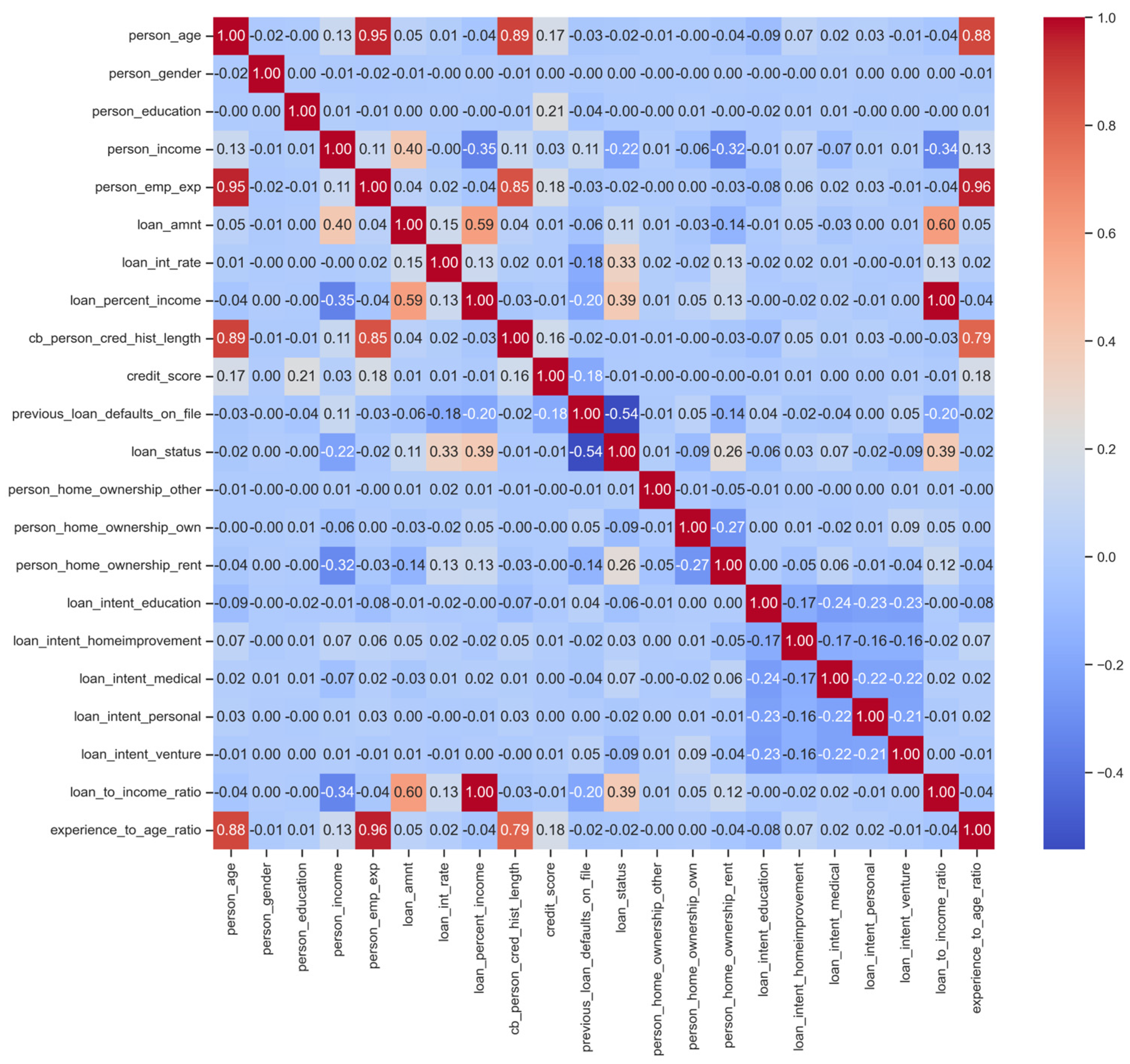
To ensure the independence of the predictor variables and mitigate the risk of multicollinearity, a feature-level correlation matrix was computed and visualized as a heatmap described in Figure 1. Multicollinearity occurs when independent variables are highly correlated with one another, which can inflate model variance, cause overfitting, and distort the subsequent SHAP feature importance calculations.

Analysis of the correlation heatmap revealed significant redundancies among several predictors. Specifically, severe collinearity was observed between person_age and person_emp_exp (employment experience), which exhibited a near-perfect correlation coefficient of 0.95. Additionally, both of these features showed high correlations (0.89 and 0.85, respectively) with cb_person_cred_hist_length. Because employment experience and credit history inherently scale with age, retaining all of these variables introduces redundant noise rather than unique predictive value. Furthermore, loan_percent_income displayed a perfect correlation (1.00) with the engineered loan_to_income_ratio feature, confirming it as a direct mathematical duplicate.

Consequently, to optimize dimensionality and preserve the mathematical stability of the ensemble models, redundant features such as person_age, person_emp_exp, and loan_percent_income were systematically dropped from the dataset. It is important to note that this correlation-based exclusion served only as a preliminary filtering step to remove explicit mathematical redundancies, rather than the definitive feature selection mechanism. Because linear correlation coefficients cannot capture complex, non-linear dependencies, the primary burden of feature selection was delegated to the ensemble algorithms themselves. Specifically, the tree-based architectures utilized in this study (Random Forest and AdaBoost) function as inherent embedded feature selection models. During the training phase, these algorithms naturally evaluate feature splits, handle non-linear interactions, and assign hierarchical importance to the remaining predictors.

In EDA stage, the prepared dataset is visualized to provide better understanding of it before training the model. Two analysis, univariate and bivariate analysis, are conducted to comprehend each variable on its own and to explore relationships between target variable, which is loan_status, and other variables.

4.3.1. Univariate Data Analysis

Univariate analysis is performed to understand the distribution of a single variable. 13 variables are analyzed in this stage and categorized into demographic information, financial and loan-related information, and engineered features.

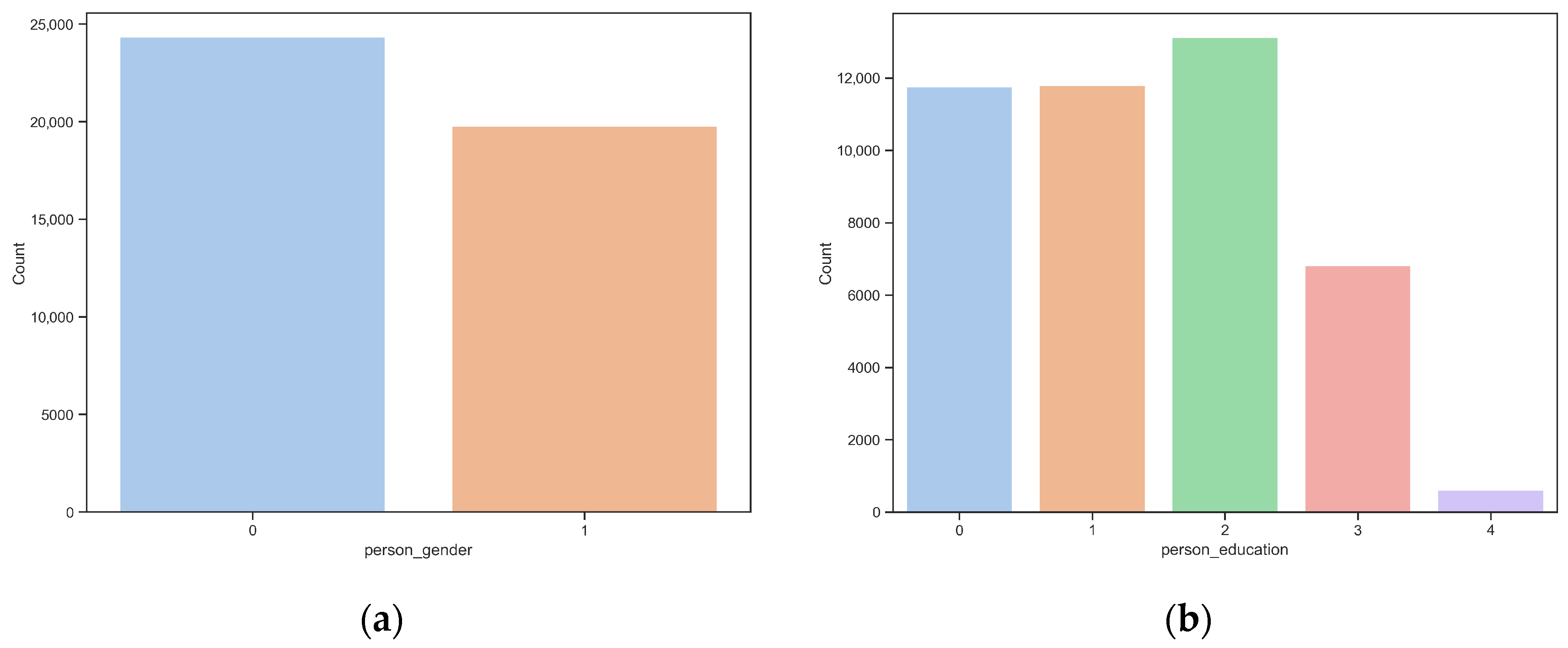
• Demographic Information: Figure 2a,b show count plots for person_gender and person_education. The gender distribution is relatively balanced, with males (0) slightly more frequent than females (1). Education levels are more unevenly distributed, most applicants hold a bachelor’s degree (2), followed by associate (1) and high school (0), while master (3) and doctorate (4) degrees are less common.

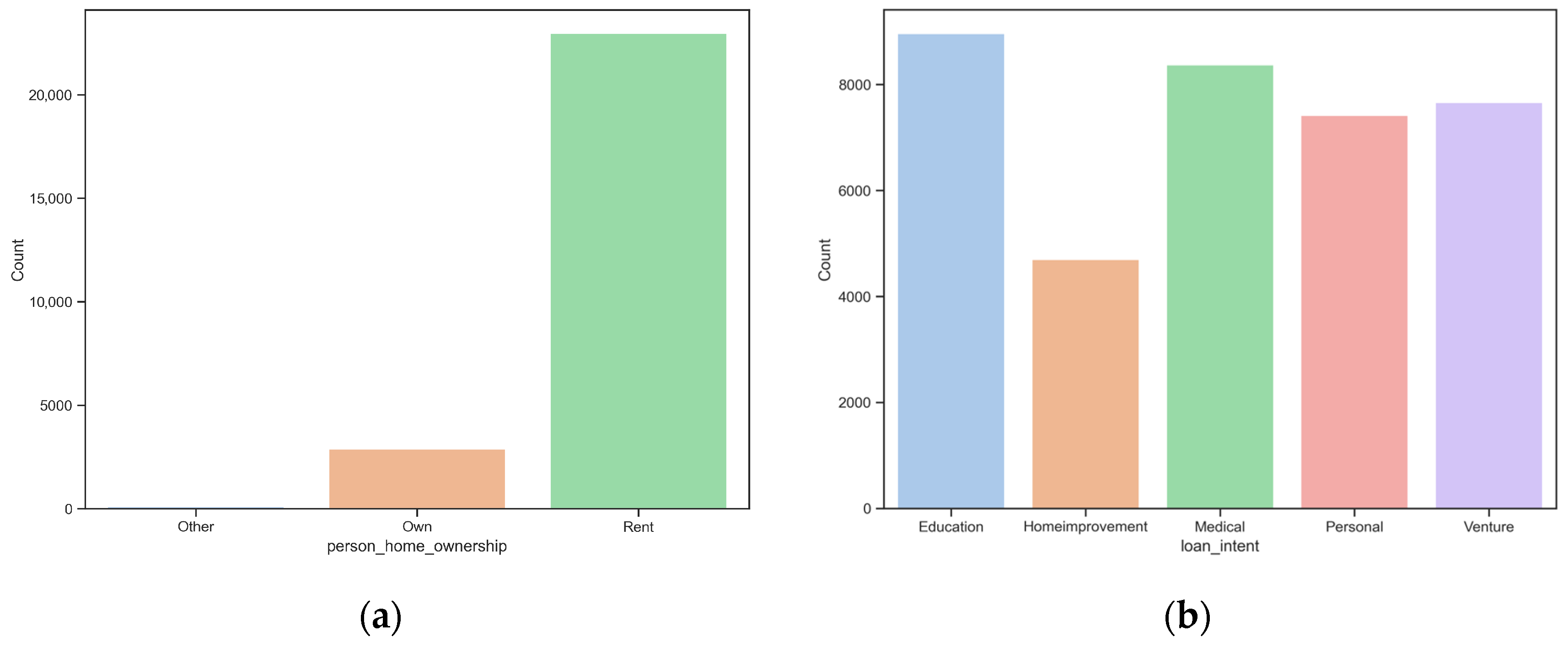
Figure 3a,b show the distributions of person_home_ownership and loan_intent. The homeownership chart reveals a highly imbalanced dataset, with most individuals owning their homes, a smaller portion renting, and very few in the other category. In contrast, loan intent is more evenly distributed across different purposes. The most common reasons for taking a loan are Education and Medical, followed by Venture and Personal, while Home Improvement is the least common. These plots provide insight into applicant profiles and the main purposes for which loans are requested.

2.

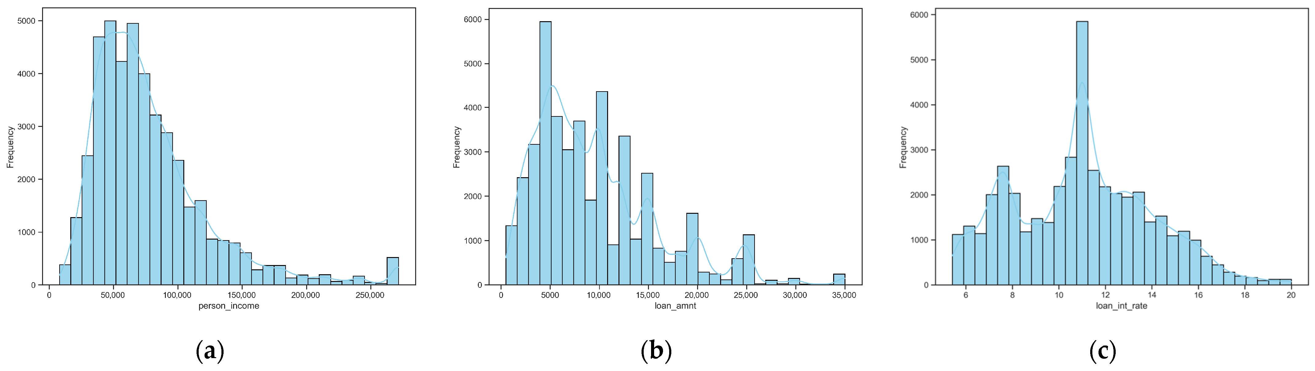
Financial and Loan-related Information: Figure 4a–c show the distributions of person_income, loan_amnt, and loan_int_rate. Most people earn a lower-to-middle income, around $50,000–$60,000, with a few earning much more, creating a long tail on the higher end. Loan amounts have several common values, with peaks at $5000 and $10,000 and smaller peaks at $12,000 and $15,000, showing that loans are usually given in standard amounts. Interest rates also have two main groups, around 7.5–8% and 11%, which likely reflect borrowers with different risk levels. The higher-rate group gradually decreases in frequency.

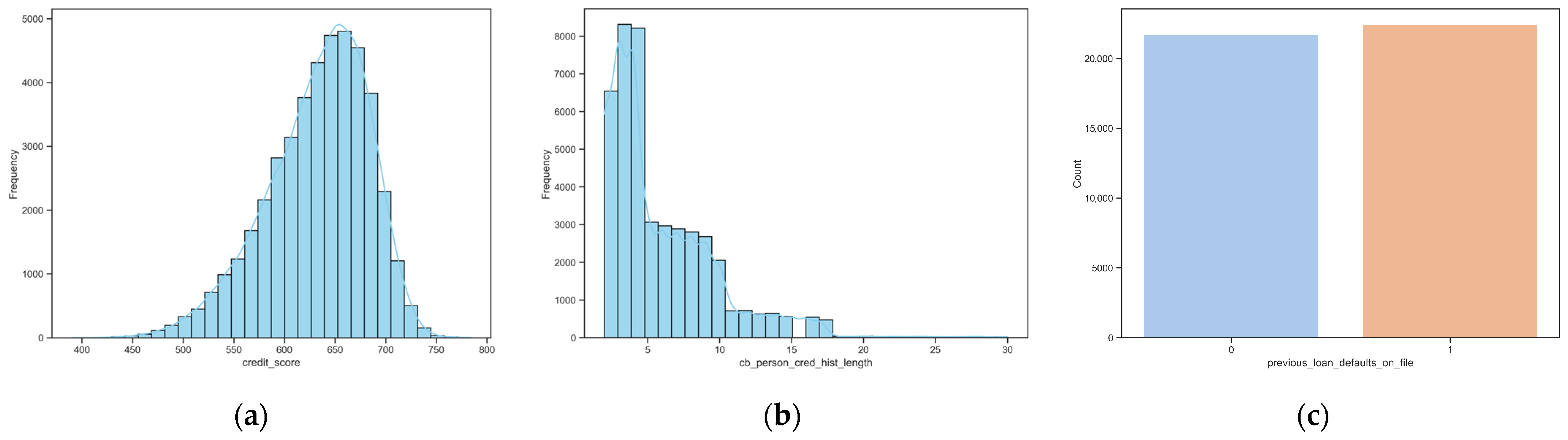
The distributions shown in Figure 5a–c show patterns in credit_score, cb_person_cred_hist_length, and previous_loan_defaults_on_file. The credit_score distribution is clearly left-skewed, with a peak in the upper 600s. This suggests that most applicants have moderately good credit profiles. At the same time, there is a noticeable long tail extending toward lower scores. This indicates the presence of a smaller group of lower-scoring outliers. Conversely, the cb_person_cred_hist_length exhibits a heavily right-skewed distribution. The massive concentration at the lower end demonstrates that most applicants have relatively short credit histories (under 5 years), with the frequency decaying rapidly as history length increases. The categorical distribution of previous_loan_defaults_on_file shows a slightly higher number of applicants with a history of defaults (1) than those with clean records (0). This suggests that defaults are relatively common in this dataset. Overall, it points to a somewhat higher-risk applicant pool than might be expected.

3.

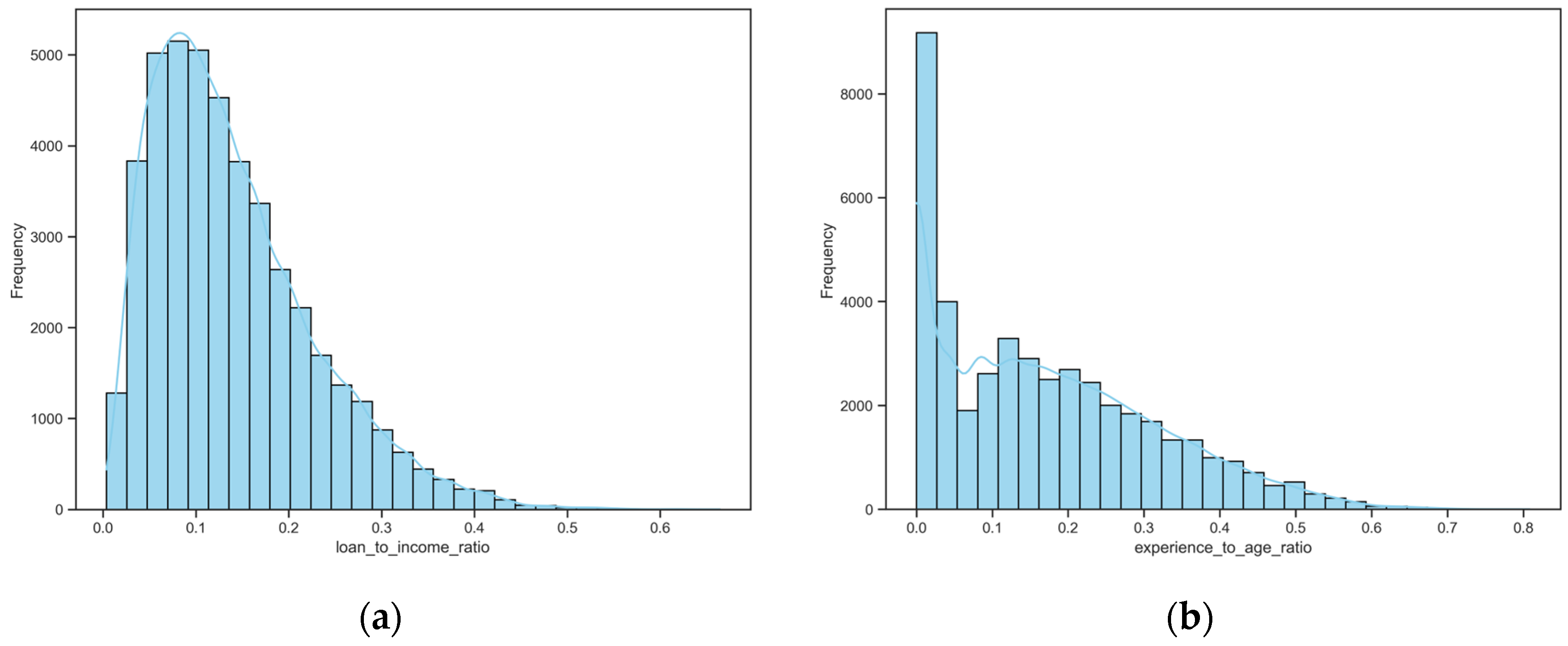
Engineered Features: Figure 6a,b show the distributions of loan_to_income_ratio and experience_to_age_ratio. The loan_to_income_ratio exhibits a distinctly right-skewed distribution. It peaks sharply around the 0.1 mark. This indicates that most applicants request loan amounts representing a relatively conservative fraction (roughly 10%) of their total annual income. Conversely, the experience_to_age_ratio displays a severe rightward skew with a massive initial concentration near zero. This sharp spike suggests a substantial cohort of applicants possesses little to no formal employment history. Beyond this initial peak, the distribution becomes multimodal and gradually tapers off. This structural irregularity highlights the natural variability in career trajectories and work experience relative to an applicant’s age.

4.3.2. Bivariate Data Analysis

Bivariate analysis is performed to understand the relationships between target variable and key variables that can influenced the model. 6 relationships are analyzed in this stage and categorized into numeric and categorical features.

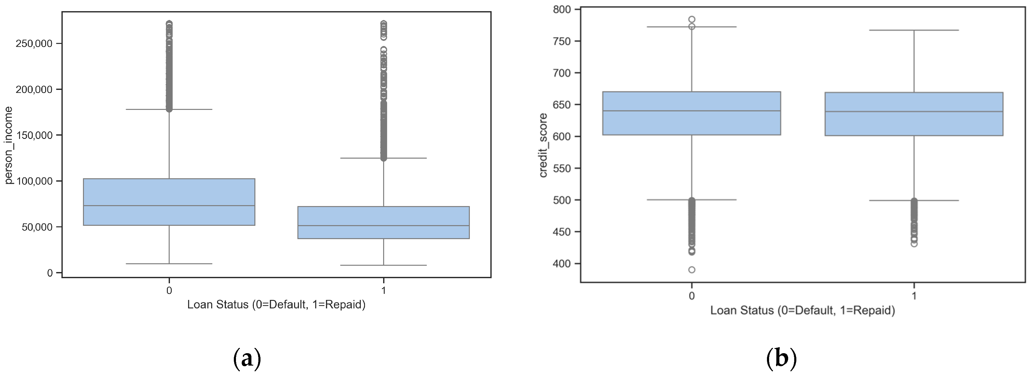
• Numeric Features: Figure 7a,b illustrate the bivariate relationship between person_income, credit_score, and loan_status. The circles plotted beyond the whiskers represent statistical outliers in the dataset. Counterintuitively, Figure 7a reveals that applicants who defaulted on their loans (Class 0) generally exhibit a higher median income than those who successfully repaid (Class 1). This inverse relationship suggests that absolute income alone cannot guarantee successful repayment, likely due to interactions with the requested loan amount. Furthermore, Figure 7b shows virtually indistinguishable credit score distributions between the two classes. Their nearly identical medians and interquartile ranges indicate that credit score is not a strong independent discriminator for predicting loan performance. Together, these findings highlight the limitations of single-variable analysis and strongly justify deploying complex ensemble models to capture deeper, non-linear feature interactions.

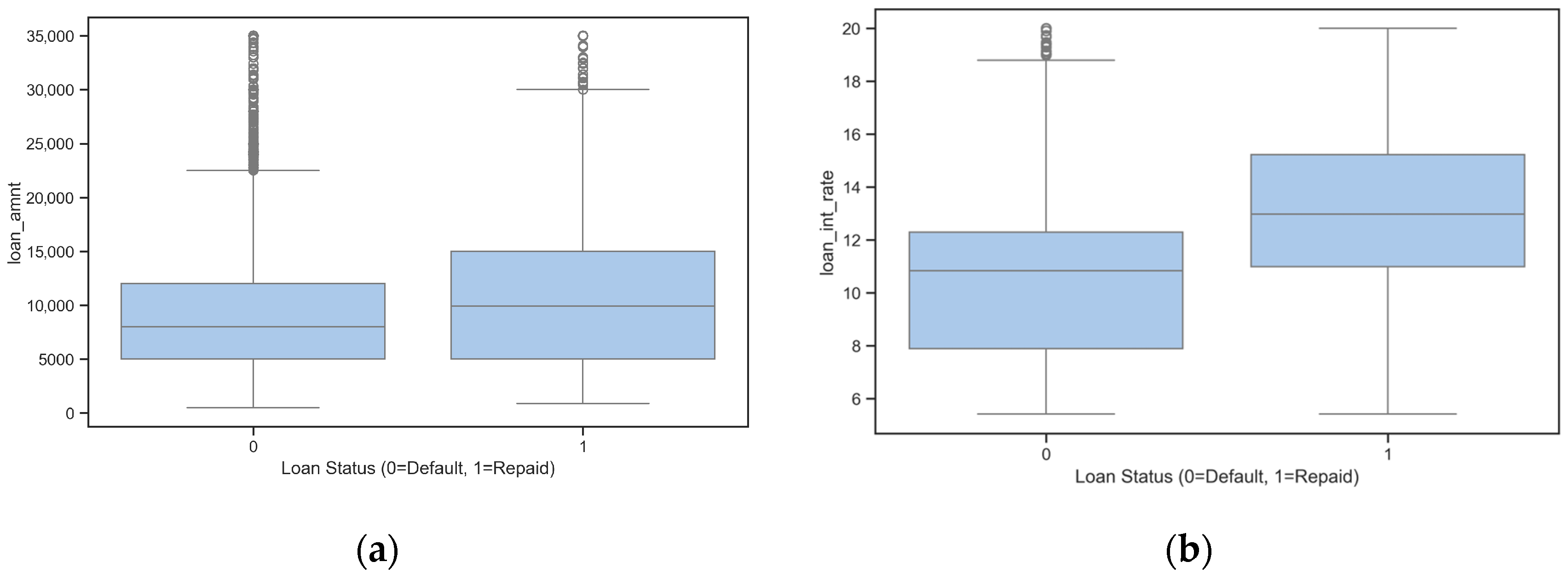
Figure 8a,b illustrate the relationship of loan_amnt and loan_int_rate with loan_status. Statistical outliers in the dataset are identified by the circular markers positioned beyond the whiskers. Figure 8a demonstrates that while the overall ranges overlap heavily, loans that were successfully repaid (Class 1) actually exhibit a slightly higher median loan amount than those that defaulted (Class 0). More strikingly, Figure 8b reveals a clear divergence in interest rates, repaid loans feature noticeably higher interest rates compared to defaulted loans. In traditional finance, higher interest rates typically correlate with higher risk and default rates. However, this dataset reveals a counterintuitive, inverse trend. This suggests that interest rates likely interact with other hidden variables to determine the final repayment outcome, further emphasizing why robust ensemble models are required to decode these complex financial patterns.

2.

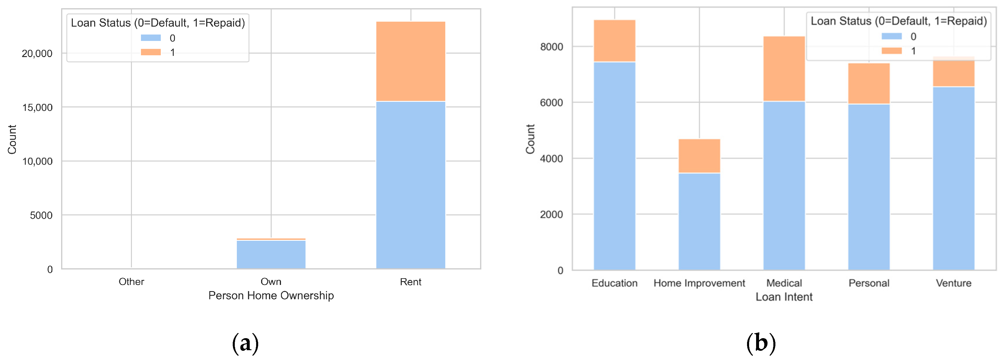
Categorical Features: Figure 9a,b illustrate the bivariate relationships between key categorical features (person_home_ownership and loan_intent) and loan_status. Figure 9a reveals a severe demographic imbalance, with the vast majority of applicants classified as renters. Across all homeownership categories, the volume of defaults (Class 0) significantly outweighs successful repayments (Class 1). Notably, applicants who own their homes represent a surprisingly small subset of the dataset and exhibit a disproportionately high default rate. Furthermore, Figure 9b demonstrates that the declared purpose of the loan also influences repayment outcomes. While defaults heavily dominate every category, the proportional ratio of defaults to repayments varies; for instance, Education and Venture loans exhibit massive default volumes, whereas categories such as Medical and Home Improvement display slightly thicker proportional repayment bands. Together, these variations confirm that categorical demographics encode valuable predictive signals, further ustifying their inclusion in the machine learning pipeline.

4.4. Handling Class Imbalance

Following the feature selection process, an analysis of the loan_status target variable revealed a significant class imbalance. The majority class (reliable borrowers) represented 77.82% of the dataset, while the minority class (defaulters) represented 22.18%. In order to avoid the occurrence of an artificial bias towards the major class in the models, an often-encountered issue which increases model accuracy at the expense of minority class recall, SMOTE and the ADASYN algorithms were used.

Crucially, to maintain methodological rigor and prevent data leakage, these methods were not applied to the dataset globally. Instead, they were strictly integrated within the subsequent k-fold cross-validation pipeline. Synthetic samples were generated exclusively on the training folds during each iteration, ensuring that the validation folds remained entirely authentic and representative of real-world, imbalanced financial distributions.

4.5. Model Development and Evaluation

After performing EDA, the dataset is almost ready to train. However, some values have higher number format compared with other features. For example, the values in loan_int_rate feature are 4000, …, 6000 but those in person_education are 0, 1, …, 5. Such a big difference of values in training dataset can create bias outcome of prediction model. Therefore, higher number values are transformed into standard values by using z-score skilling.

In order to effectively assess the predictive accuracy as well as generalize the results obtained, 5-Fold Stratified Cross-Validation was employed. In this way, the initial ratio within the class distributions in the data, where there was an extreme 78:22 imbalance skewed heavily towards loan default (Class 0), was maintained. Crucially, to prevent data leakage during the cross-validation process, all scaling and class-balancing treatments were embedded directly into modular machine learning pipelines. Within these pipelines, synthetic minority oversampling techniques, SMOTE and ADASYN, were dynamically applied exclusively to the training subsets of each fold. This synthesized the minority repaid class (Class 1) to mitigate the model’s inherent rejection bias without contaminating the validation data.

These preprocessing pipelines were seamlessly integrated with four diverse ensemble classifiers: Random Forest (Bagging), AdaBoost (Boosting), and custom Stacking and Voting ensembles consisting of Logistic Regression, K-Nearest Neighbors, and Decision Tree base learners. This systematic architecture allowed for a mathematically sound, comparative evaluation of how different adaptive resampling techniques influence predictive capabilities under rigorously controlled conditions.

4.5.1. Model Performance Metrics

Table 6. Evaluation of Training Model.

Model	Resampling	Accuracy	Precision	Recall	F1-Score	AUC
Bagging	SMOTE	0.9147 ± 0.0021	0.7840 ± 0.0066	0.8498 ± 0.0062	0.8155 ± 0.0043	0.9719 ± 0.0019
	ADASYN	0.9033 ± 0.0020	0.7363 ± 0.0030	0.8789 ± 0.0071	0.8013 ± 0.0044	0.9706 ± 0.0017
Boosting	SMOTE	0.8744 ± 0.0029	0.6610 ± 0.0075	0.8908 ± 0.0090	0.7588 ± 0.0037	0.9599 ± 0.0021
	ADASYN	0.8403 ± 0.0025	0.5867 ± 0.0045	0.9474 ± 0.0063	0.7246 ± 0.0028	0.9579 ± 0.0017
Stacking	SMOTE	0.8958 ± 0.0047	0.7435 ± 0.0100	0.8096 ± 0.0117	0.7751 ± 0.0102	0.9572 ± 0.0023
	ADASYN	0.8819 ± 0.0036	0.6856 ± 0.0093	0.8638 ± 0.0099	0.7644 ± 0.0057	0.9556 ± 0.0021
Voting	SMOTE	0.8864 ± 0.0036	0.6944 ± 0.0071	0.8710 ± 0.0067	0.7727 ± 0.0069	0.9597 ± 0.0023
	ADASYN	0.8714 ± 0.0031	0.6522 ± 0.0066	0.9004 ± 0.0045	0.7564 ± 0.0045	0.9564 ± 0.0020

describes the evaluation of the trained models, comparing their performance in terms of Accuracy, Precision, Recall, F1-score and Area Under the Curve (AUC) under 5-folds cross-validation using the resampling techniques such as SMOTE and ADASYN to show how well each model predicts loan approval outcomes.

Overall, in the context of credit risk assessment, standard classification metrics must be interpreted through the lens of institutional financial impact. Therefore, this study evaluates model performance with a specific focus on the trade-off between Precision and Recall. Precision represents the model’s ability to minimize False Positives (predicting a loan will be repaid when it actually defaults). In banking, a false positive is the most critical error, as approving a high-risk applicant leads directly to non-performing loans and severe capital loss. Conversely, Recall represents the model’s ability to minimize False Negatives (predicting a loan will default when it would have been repaid). While less immediately destructive than a capital default, excessive false negatives carry a significant business opportunity cost through lost interest revenue, customer dissatisfaction, and the unfair exclusion of reliable borrowers.

The tension between these metrics forms the core of a bank’s risk appetite, and the results clearly illustrate this inherent Precision-Recall trade-off when treating financial data imbalance. Balancing techniques heavily influenced this dynamic: the application of ADASYN consistently maximized Recall across all ensemble architectures at the expense of Precision. Most notably, the Boosting model paired with ADASYN achieved the highest overall Recall (0.9474). While this configuration aggressively prioritizes minimizing unfair rejections (False Negatives), it does so at the unacceptable business cost of severely diminished Precision (0.5867), which would lead to an increase in costly false approvals.

Conversely, the Bagging model paired with SMOTE delivered the most reliable performance, achieving an optimal business equilibrium. It recorded the highest overall Accuracy (0.9147), Precision (0.7840), F1-Score (0.8155), and AUC (0.9719). This indicates that the Bagging architecture is exceptionally capable of maintaining high predictive accuracy, protecting institutional capital through high Precision, while securing enough Recall to ensure profitable lending volume, all without heavily biasing toward the majority class.

Furthermore, to ensure the statistical credibility of the comparative model analysis, performance metrics are supported by standard deviations and 95% confidence intervals derived from the stratified k-fold cross-validation process. The exceptionally low variance observed across all metrics, such as an AUC standard deviation of just ±0.0019 for the top-performing Bagging-SMOTE model, proves the robust stability of the proposed framework. This confirms that the superior discriminative ability of the Bagging architecture is statistically significant, mathematically reliable, and not dependent on a single, randomized data split.

4.5.2. Confusion Matrix Analysis

A comparative analysis of the confusion matrices for the SMOTE-balanced, described in

Table 7. Consolidated Confusion Matrices for SMOTE-Balanced Ensemble Models.

Method	Actual Result	Predicted Result
		Default	Repaid
Bagging	Default	32,042	2292
	Repaid	1470	8316
Boosting	Default	29,861	4473
	Repaid	1069	8717
Stacking	Default	31,600	2734
	Repaid	1863	7923
Voting	Default	30,582	3752
	Repaid	1262	8524

, and ADASYN-balanced, described in

Table 8. Consolidated Confusion Matrices for ADASYN-Balanced Ensemble Models.

Method	Actual Result	Predicted Result
		Default	Repaid
Bagging	Default	31,254	3080
	Repaid	1185	8601
Boosting	Default	27,801	6533
	Repaid	515	9271
Stacking	Default	30,455	3879
	Repaid	1333	8453
Voting	Default	29,633	4701
	Repaid	975	8811

, ensemble models reveals exactly how each resampling technique alters classification behavior. By addressing the dataset’s inherent imbalance, all models successfully shifted away from their initial bias of defaulting to majority-class (default) predictions.

Under the SMOTE configuration, the Bagging model demonstrates the most operationally sound and balanced discrimination. It achieves the highest success rate in correctly identifying high-risk applicants, successfully classifying 32,042 Actual Default instances. More importantly for banking risk management, it produces the lowest number of costly false approvals (predicting Actual Default cases as Repaid) at only 2292 instances. Concurrently, it maintains a strong capability in identifying reliable borrowers (8316 True Repaid).

Conversely, the ADASYN-balanced models behave far more aggressively in predicting the minority class (Repaid loans), significantly reducing the rate of false rejections (predicting Actual Repaid cases as Default) but at the direct cost of increased false approvals. This trade-off is most heavily pronounced in the Boosting model under ADASYN. While it achieves the absolute highest detection of reliable borrowers, correctly identifying 9271 Actual Repaid cases with a remarkably low 515 false defaults, this extreme sensitivity severely compromises precision. It falsely approves 6533 Actual Default loans, which represents an unacceptable level of credit risk for most financial institutions.

Ultimately, while the ADASYN-Boosting configuration is unparalleled in preventing the unfair rejection of reliable candidates, the confusion matrices confirm that the SMOTE-Bagging configuration provides the safest operational threshold. It minimizes institutional exposure to risky defaults while still maintaining highly accurate and fair approval rates.

4.5.3. Receiver Operating Characteristic (ROC) Curve Comparison

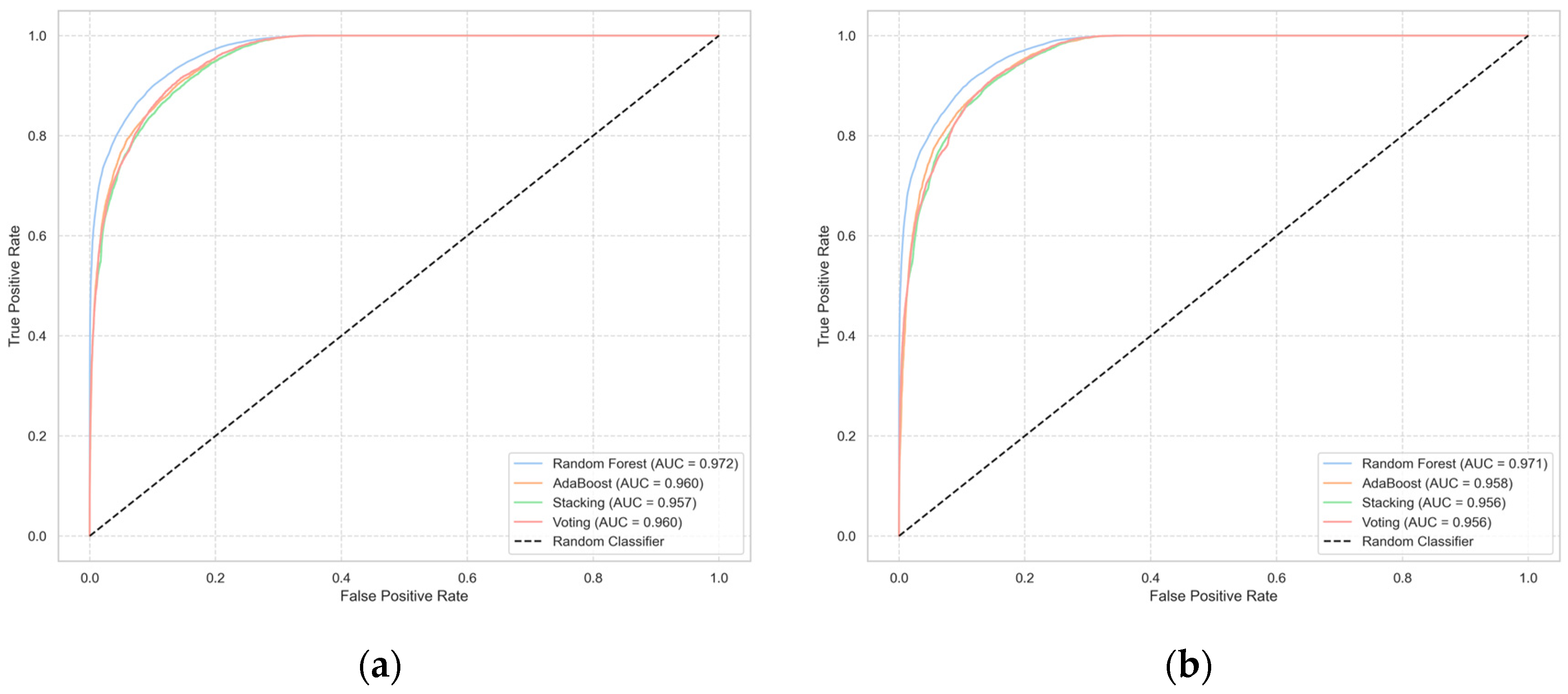
Figure 10a,b illustrate the Receiver Operating Characteristic (ROC) curves for the SMOTE- and ADASYN-balanced models, respectively. As depicted in the visualizations, the Bagging architecture achieves the highest Area Under the Curve (AUC), scoring an impressive 0.972 under the SMOTE configuration and a nearly identical 0.971 under ADASYN. This indicates a superior, highly robust discriminative ability in distinguishing between the default and repaid classes. Although all four ensemble architectures perform exceptionally well, maintaining strong AUC scores above 0.95 across both synthetic resampling techniques, the Bagging model exhibits a distinct, measurable advantage in overall predictive probability and classification performance.

Crucially, these performance metrics must be interpreted through the lens of operational business impact. While the incremental ROC-AUC improvements between the top-performing ensemble architectures may appear mathematically marginal, such as the Bagging model (0.972) outperforming the Voting meta-ensemble (0.960) by a factor of 0.012, this difference carries profound financial significance. The ROC-AUC measures the model’s overall ability to rank-order risk. At the scale of retail banking, a 0.012 improvement in discriminative power means the model significantly excels at separating borderline applicants who share similar demographic and financial profiles. In a high-volume lending environment, capturing these edge cases directly reduces the False Positive Rate at the operational decision threshold. Therefore, the seemingly marginal statistical gain of the SMOTE-Bagging configuration translates to a quantifiable reduction in non-performing loans, preventing compounding capital loss and ensuring institutional financial security.

4.6. SHAP-Based Interpretability Analysis (XAI)

SHAP has been applied in this study to be transparent and improve interpretability of the model. It is widely used to interpret complex black box models because it provides a unified and consistent measure of exactly how much, and in which direction, each input variable influenced the result.

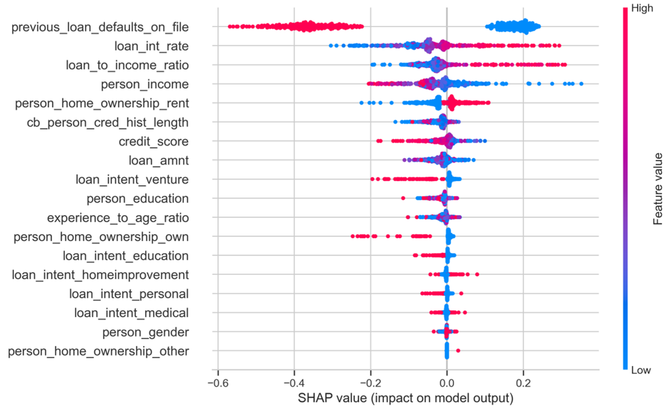
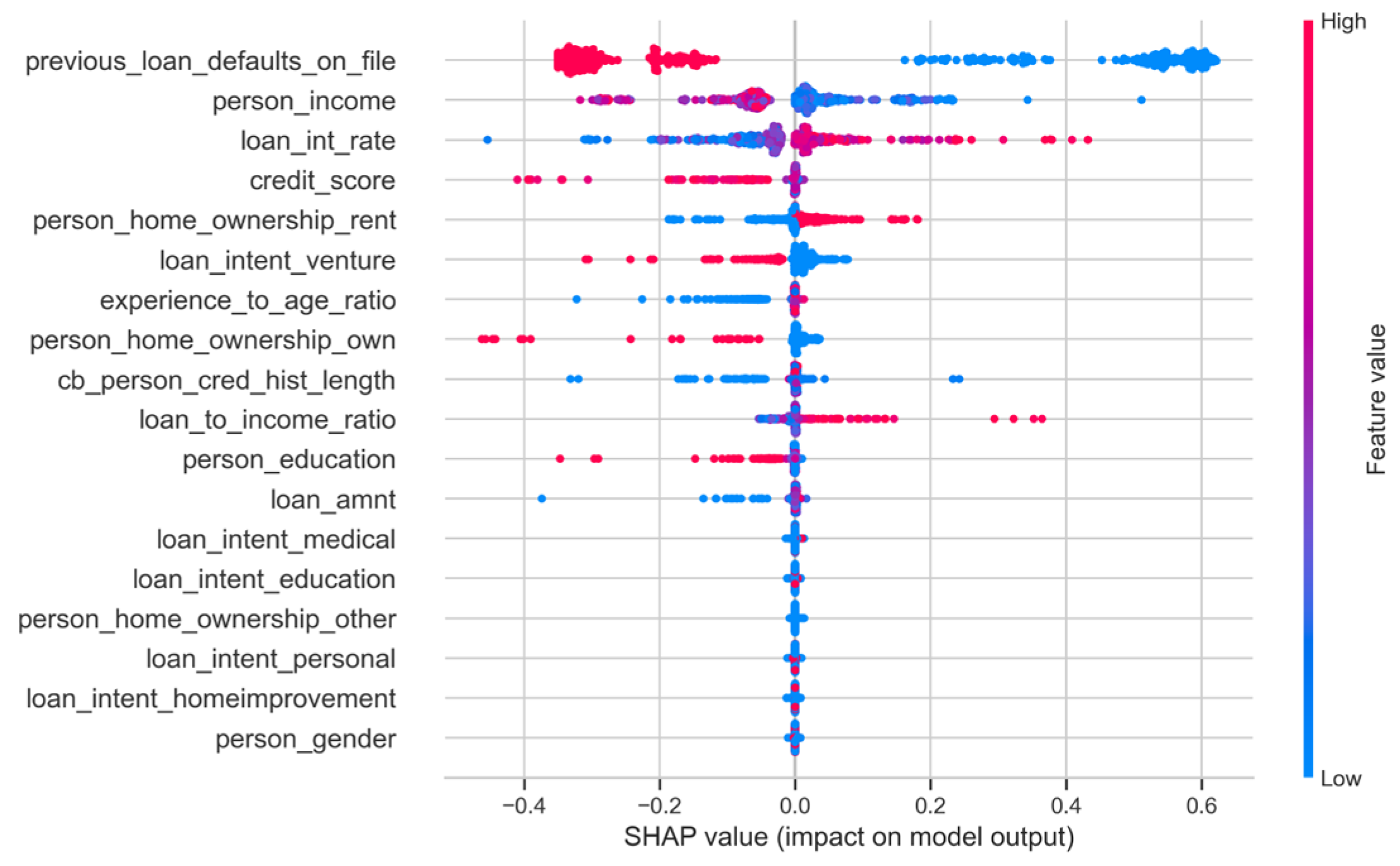
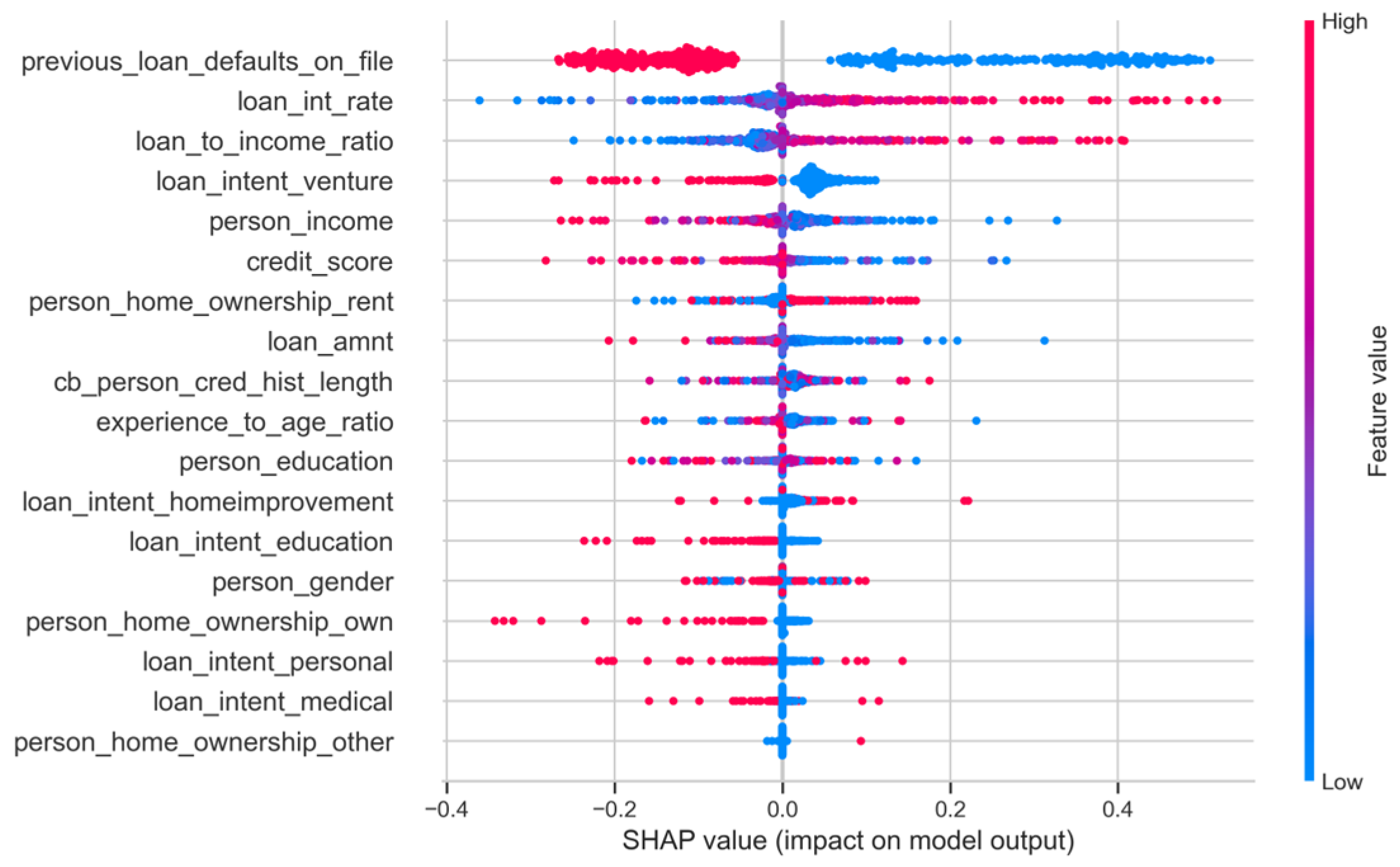
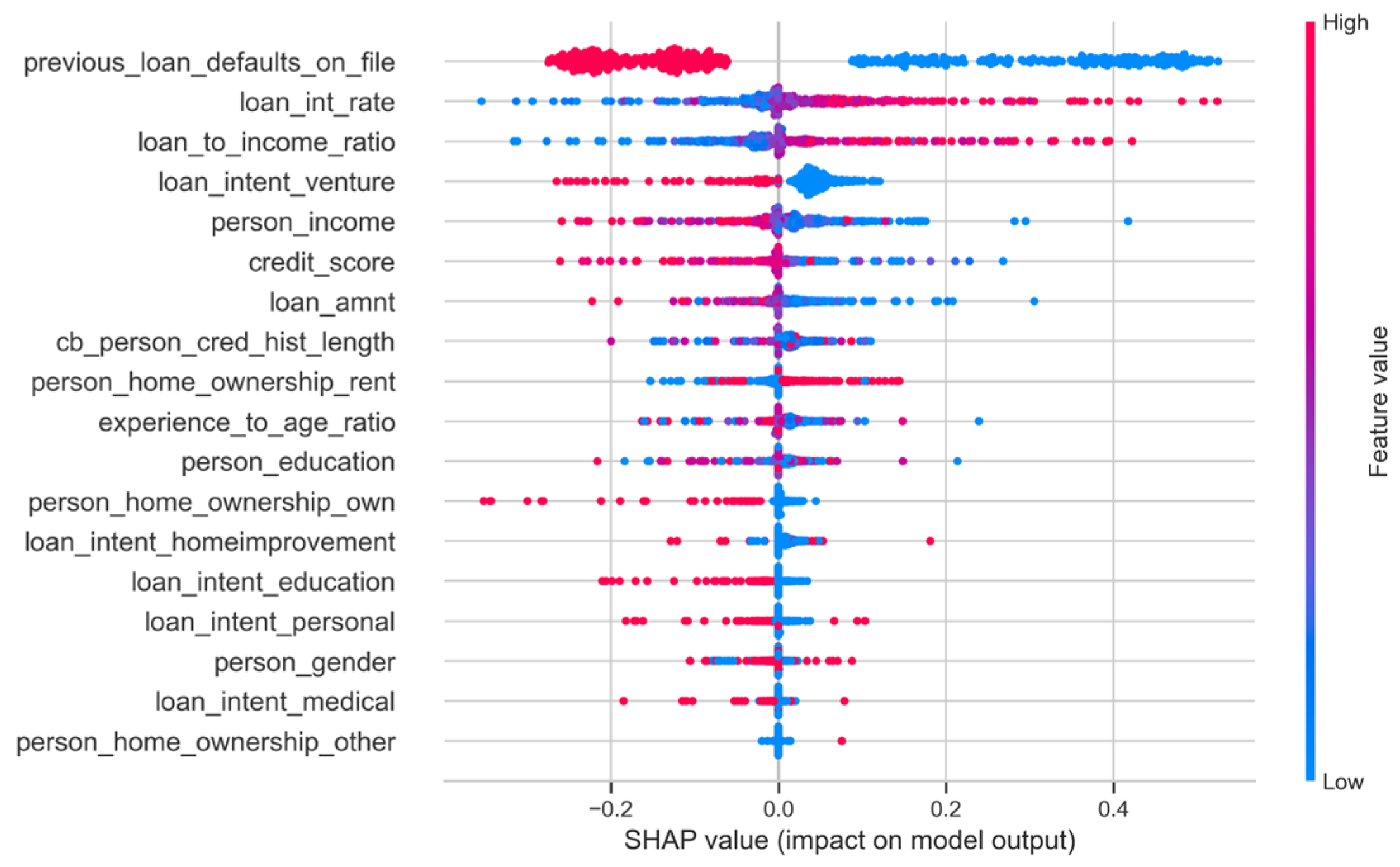
Given the superior predictive performance of the SMOTE-resampled models over their ADASYN counterparts during cross-validation, the interpretability analysis was exclusively focused on these optimal configurations. Due to the prohibitive computational cost of generating SHAP values for advanced meta-learner, particularly the Stacking and Voting classifiers, a statistically representative random sample of 500 instances was utilized for this analysis.

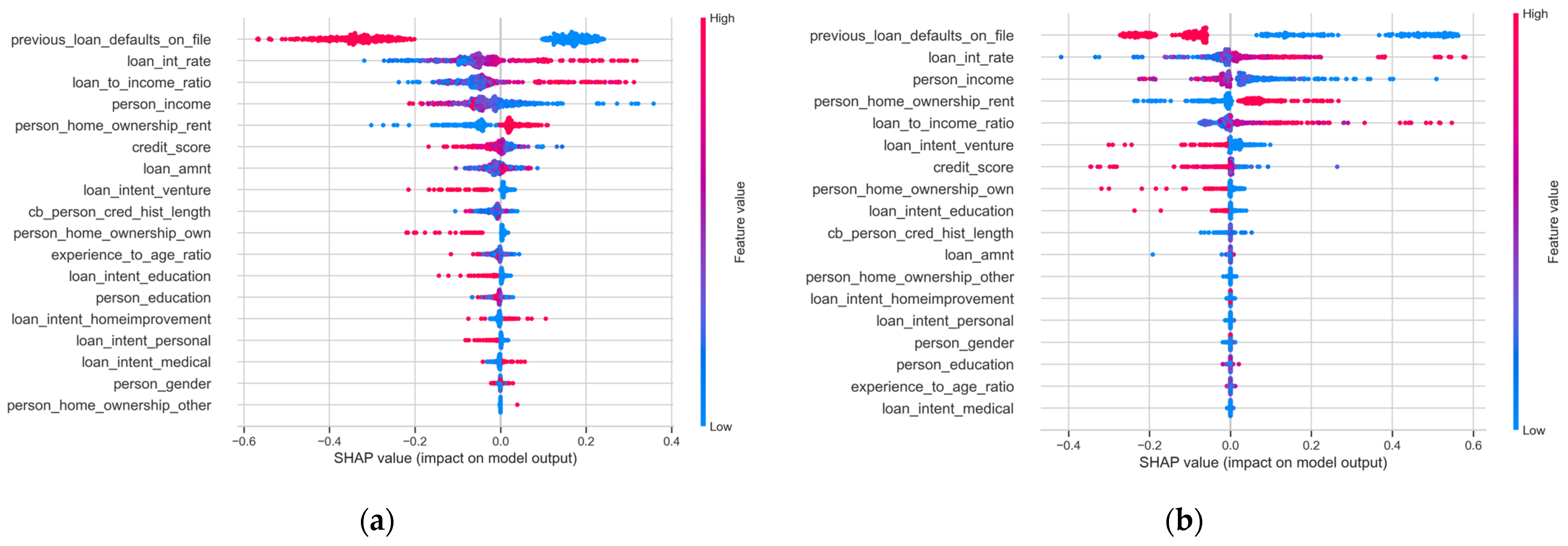
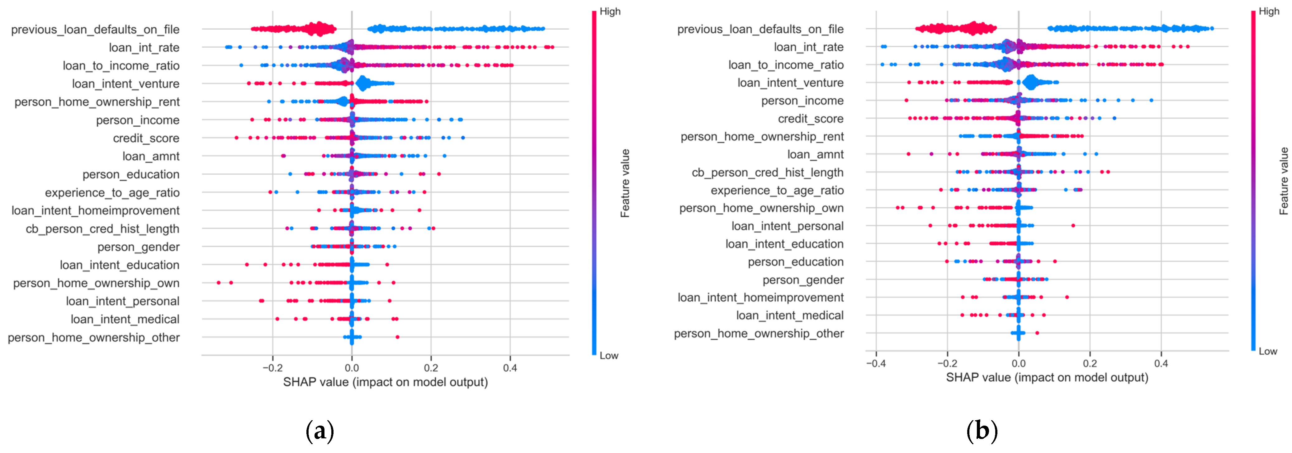
Analysis of the global SHAP summary plots, Figure 11 and Figure 12, reveals a strong consensus among all four SMOTE-balanced ensemble architectures regarding the primary drivers of loan performance.

Across every model, previous_loan_defaults_on_file emerges as the absolute most significant predictor. The visualizations clearly demonstrate that the presence of a default history (indicated by the high-value red data points) exerts a massive negative impact on the model output, strongly driving the prediction toward a ‘Default’ classification. Following this, core financial metrics, specifically loan_int_rate, loan_to_income_ratio, and person_income, form the secondary tier of predictive importance.

Across all architectures, higher absolute incomes consistently shift predictions toward successful repayment, while the models exhibit acute sensitivity to high loan-to-income proportions and elevated interest rates, which push predictions toward default. While the Bagging and Boosting base estimators exhibit highly concentrated feature attribution on these top-tier variables, the Stacking and Voting meta-ensembles demonstrate a slightly broader distribution of feature importance, successfully synthesizing the logic of their underlying algorithms.

Most importantly, across all four predictive architectures, demographic attributes such as person_education and person_gender consistently anchor the bottom of the feature hierarchy. Their SHAP values are clustered tightly around zero, indicating a negligible role in the decision-making process. This confirms that the ensemble framework relies entirely on logical, finance-driven behavioral data rather than demographic identifiers. This alignment between high predictive performance (evidenced by the Bagging model’s peak AUC of 0.972) and transparent, unbiased feature attribution effectively resolves the ‘black-box’ challenge, providing the rigorous accountability required for deployment in modern financial institutions.

5. Discussion

This study evaluated four interpretable ensemble machine learning frameworks for credit risk assessment. The SMOTE-balanced Bagging model (Random Forest) emerged as the optimal configuration, achieving a peak AUC of 0.972. Beyond raw predictive accuracy, integrating post-hoc SHAP analysis resolved the black-box dilemma, confirming that the model relies on logical financial behaviors (e.g., default history, loan-to-income ratio) rather than arbitrary demographic variables. Practically, this configuration establishes the safest operational threshold for banks, minimizing costly false approvals while maintaining profitable lending volumes. Furthermore, generating local and global SHAP explanations enables loan officers to issue transparent, feature-justified credit decisions rather than blind approvals.

Transitioning this framework into real-world banking IT infrastructures is best achieved via a decoupled microservices architecture. This ensures operational cost-efficiency by allowing resource-intensive model retraining to occur in scheduled offline batches, while maintaining a low-latency pipeline for daily credit inference. Additionally, deployment must strictly navigate global data privacy frameworks (e.g., General Data Protection Regulation (GDPR)) through cryptographic anonymization. From a regulatory standpoint, the SHAP-enhanced architecture directly satisfies the stringent governance requirements of upcoming legislation like the EU AI Act, empowering institutions to audit algorithmic decisions, detect proxy biases, and legally justify adverse actions to regulatory bodies.

Finally, this framework actively advances the United Nations Sustainable Development Goals (SDGs). By empirically proving that the optimized Bagging model assigns near-zero predictive weight to demographics like gender and education, the system mitigates explicit algorithmic bias and reduces structural inequalities in credit access (SDG 10). Concurrently, safely expanding credit to reliable borrowers, while protecting institutional infrastructure from catastrophic defaults, fosters the transparent and sustainable financial inclusion required for equitable economic growth (SDG 8).

6. Limitations and Future Study

This study successfully combines an interpretability framework while also addressing data imbalance using SMOTE and rigorous cross-validation. However, several limitations still exist. One key issue is the reliance on a single public dataset, which limits how well the results can be applied in real-world settings. Since the data does not capture specific geographic, socio-economic, or economic conditions, the model’s generalizability remains uncertain. To improve this, future research should test and adapt these models using real-world financial data. Incorporating dynamic, behavioral, or time-based variables could also enhance predictive performance. In addition, the current evaluation does not consider the unequal costs of errors. In practice, approving a loan that later defaults is far more costly than rejecting a reliable borrower. Future studies should therefore apply cost-sensitive learning to better reflect real banking risks.

Moreover, in future research, more detailed XAI (Explainable AI) examples should be included, for example, using SHAP waterfall charts, which will provide an understanding of the way the model decision-making affects the individual candidates. While demographic variables such as gender and education play little to no role according to the results of the SHAP analysis, this does not completely exclude the possibility of any bias. For purposes of ensuring fairness and particularly in respect to SDG 10, it is important that such models be subjected to fairness tests, for instance Demographic Parity or Equalized Odds before actual application.

7. Conclusions

This research successfully addressed the performance-transparency trade-off in automated lending by evaluating four ensemble machine learning architectures—Bagging, Boosting, Stacking, and Voting—integrated with advanced data resampling techniques (SMOTE and ADASYN) and a SHAP-based Explainable AI (XAI) framework. While all ensemble models demonstrated high discriminative power, the SMOTE-balanced Bagging (Random Forest) model emerged as the superior performer for credit risk prediction. Achieving a peak AUC of 0.972, this configuration established the safest operational threshold for banking risk management by strictly minimizing costly false approvals while maintaining a high identification rate of reliable borrowers.

Crucially, the integration of SHAP resolved the black-box challenge traditionally associated with complex meta-learning algorithms. The comparative analysis revealed a strong consensus across all four architectures: the models inherently prioritize logical financial indicators, specifically default history, interest rates, and loan-to-income ratios, while correctly assigning negligible predictive weight to demographic traits such as gender and education. This empirical validation confirms that high-performance ensembles can make decisions based purely on financial behavior rather than biased demographic profiling.

Despite these successes, the reliance on a statically sampled public dataset limits the immediate external validity of the findings, and the current framework does not account for the asymmetric variable costs of real-world misclassifications. Future research must focus on validating these architectures using diverse, longitudinal banking data and incorporating cost-sensitive learning algorithms to dynamically adjust to specific institutional risk tolerances. Furthermore, integrating counterfactual explanations could provide actionable feedback for rejected applicants.

Ultimately, this study demonstrates that high-performance machine learning can be made fully transparent, accountable, and fair. By providing clear, feature-level justifications for automated credit decisions, financial institutions can deploy advanced predictive systems that strictly comply with modern regulatory standards. Consequently, this framework directly advances SDG 10 by mitigating systemic algorithmic bias and promotes SDG 8 by fostering the transparent, sustainable financial inclusion required for equitable economic growth.