Does Mandatory ESG Disclosure Move Stock Prices? Evidence from the European Union’s Corporate Sustainability Reporting Directive

Abstract

The Corporate Sustainability Reporting Directive (CSRD) extends mandatory, assured and standardised sustainability reporting to a European reporting population several times larger than that of its predecessor, on the premise that such disclosure is priced by capital markets. This paper examines whether equity prices responded to the five legislative and standard-setting milestones through which the mandate became public between April 2021 and July 2023. German DAX constituents falling within the scope of Article 19a are compared with matched S&P 500 firms, using an annual difference-in-differences design and a daily market model event study. The annual estimator yields a positive and significant coefficient of +0.204 that is robust to alternative specifications, standard error corrections and influence diagnostics. Four diagnostics nevertheless indicate that it does not identify a regulatory effect: the same design applied to year pairs containing no CSRD or ESRS event yields estimates of comparable magnitude and mixed sign; parallel pre-trends are rejected; the coefficient is concentrated among poorly matched firm pairs and falls to +0.046 once a caliper is imposed; and the design is underpowered for effects of the magnitude it reports. The event study, which measures each firm against its own home market and therefore does not rely on the cross-country comparison, detects no abnormal return at any milestone once multiple testing and cross-sectional dependence are taken into account: the cumulative 3-day reaction across all five events is +0.8 percentage points, with a 95% confidence interval of [−2.5, +4.0], which excludes a repricing of the magnitude the annual estimate implies. The paper contributes a set of design diagnostics that distinguish an identified estimate from one that is merely stable, and shows that the two-country annual comparisons common in this literature do not survive them.

1. Introduction

The European Union has made disclosure the central instrument of its sustainable-finance policy. The reasoning behind that choice is a chain of causation rather than a single step. Mandatory, standardised and independently assured sustainability information is expected to give investors a clearer view of which firms carry climate and social risk; that clearer view is expected to be reflected in the prices those investors pay; the resulting differences in the cost of capital are expected to reward firms that manage such risks well and penalise those that do not; and the prospect of that reward is expected, in turn, to change what firms actually do. The Corporate Sustainability Reporting Directive is the most ambitious application of this logic attempted in any jurisdiction. It extends mandatory sustainability reporting to a reporting population several times larger than its predecessor, subjects that reporting to assurance for the first time, and standardises it through the European Sustainability Reporting Standards.

The chain has a first link, and that link is empirical. If a far-reaching mandate is announced and relative prices do not move, then at the moment of announcement, the capital market channel is not observably operating. The scope of that inference requires precision. A null announcement effect does not falsify the causal premise of mandatory sustainability reporting. Prices may already have impounded the mandate through earlier signals; the effect may be concentrated at implementation rather than at announcement; the channel may operate through the cost of debt, liquidity, or real corporate behaviour rather than through equity returns; and an effect too small for a given design to resolve is not an effect of zero. What an announcement study can test is narrower, and is still worth testing whether each successive resolution of legislative and technical uncertainty produced a discrete, incremental repricing of exposed firms relative to comparable unexposed ones. This is the question asked in this paper, and we confine our conclusions to it.

The literature that has sought to answer this question has not done so. Studies relating ESG disclosure and performance to stock returns report positive, negative and statistically insignificant associations in roughly equal measure, and the pattern persists in the narrower body of work that examines disclosure mandates specifically. The conventional reading of this record attributes the dispersion to genuine heterogeneity: different jurisdictions, different enforcement regimes, different periods, different measures. We advance a less comfortable possibility, and the paper is organised around testing it rather than asserting it. Much of the dispersion may be manufactured by a research design that the literature holds in common. Disclosure mandates are enacted by states, so a researcher who wants a control group of unregulated firms is obliged to look abroad. The resulting comparison—regulated firms in one country against unregulated firms in another, before and after the rule changes—quietly absorbs every difference in monetary policy, energy costs, exchange rates, sectoral composition and investor sentiment between the two economies into the coefficient of interest. Those differences are large, and they are not stable from one year to the next.

Our setting allows this concern to be examined directly rather than raised as a caveat. The European Commission published its CSRD proposal on 21 April 2021; the Directive was adopted in December 2022 and the first reporting standards in July 2023. We compare the constituents of the German DAX, all of which fall within the scope of the Directive, with S&P 500 firms matched on sector, employees, levered beta and market capitalisation. Our strategy proceeds in two stages. We first estimate the design that this literature conventionally uses and subject it to the robustness checks the literature conventionally applies. We then ask a question that is rarely put: whether the number that design produces carries any information about the regulation at all.

The conventional estimator returns +0.204, with a confidence interval excluding zero, and it is stable under heteroskedasticity-consistent, firm-clustered and wild-bootstrap procedures, under winsorisation, under alternative control sets, and under the removal of any single firm. By the standards routinely applied in this field, it looks robust. Four diagnostics nonetheless establish that its stability carries no information about the regulation. First, the estimate is concentrated among the least comparable matched pairs: restricting the sample to pairs within one pooled standard deviation on the matching covariates reduces it from +0.204 to +0.046, with a p-value of 0.757. Second, when every calendar year pair is classified against the full five-event chronology rather than against the April 2021 proposal alone, only five of the nine adjacent pairs are genuinely free of CSRD and ESRS events; the identical design applied to those five return estimates averages 0.225 in absolute value, larger than the CSRD window estimate, with three of five being significant at conventional levels. Third, a 9-year panel rejects the parallel trends assumption on which the design depends. Fourth, the design is severely underpowered for effects of the size at issue: its minimum detectable effect at 80% power is 23.1 percentage points, so a significant estimate from it would on average overstate a true effect of two percentage points by roughly an order of magnitude and would carry the wrong sign about a quarter of the time. Fifth, the estimate is large among firms that happened to belong to the index and indistinguishable from zero among equally in-scope firms that did not, so it splits on index membership rather than on regulatory reach. A daily event study, which measures each firm against its own home market and is therefore not exposed to the cross-country comparison, finds no reaction at any of the five milestones once multiplicity and cross-sectional dependence are taken into account.

Three contributions follow. The first is substantive: across the five CSRD and ESRS milestones, we find no detectable incremental repricing of in-scope firms, and we bound how large an average reaction the data can exclude rather than asserting that the reaction is zero. The second is methodological. An estimate can pass every robustness check this literature customarily applies while identifying nothing, because those checks test whether an estimate is stable rather than whether it means anything, and because they are computed at a level of aggregation at which the treatment was never assigned. The third is interpretive: if cross-country comparisons over annual horizons have a sampling distribution centred on whatever the differential country shock happened to be, then the inconsistency of the mandatory disclosure literature is partly an artefact of how it has been studied, and the remedy is design discipline rather than a further accumulation of estimates.

The findings bear on practice in a mainly cautionary way, and their reach is limited by what an announcement study can establish. We find no evidence that the market capitalised anticipated compliance costs, or rewarded reporting readiness, at any of the five milestones; we cannot rule out reactions smaller than the bounds our tests can resolve, and we do not claim to have tested the regime’s effects once reporting actually began. Investors should be slow to attribute return differences between European and American firms over 2021 and 2022 to the Directive, since differences of comparable size arose in years containing no CSRD event at all. Policymakers and standard-setters weighing the current simplification proposals will find that market-based evidence drawn from cross-country comparisons over this window is too weakly identified to support an argument in either direction, which is a statement about the quality of that evidence and not an argument for or against the mandate itself.

The remainder of the paper is organised as follows. Section 2 sets out the regulatory background, develops the theoretical channels through which a disclosure mandate might be priced, and shows why the existing evidence has been unable to adjudicate between them. Section 3 describes the data, their construction and the four empirical designs. Section 4 presents the results. Section 5 discusses what they imply for the interpretation of this literature, and Section 6 concludes.

2. Institutional Background and Theoretical Framework

2.1. The Escalation of European Disclosure Regulation

European sustainability reporting policy has evolved through a sequence of steps, each one more binding than the last, and the direction of travel is more informative than any single instrument. The Green Paper on corporate social responsibility of 2001 and the European Transparency Initiative of 2005 encouraged firms to report voluntarily. Voluntary reporting duly expanded, but it expanded selectively: firms disclosed what favoured them and omitted what did not. Evidence on ESG controversies documents the consequence. Controversies damage reputation and depress prices (Xue et al., 2023), the Volkswagen emissions scandal being the most conspicuous European instance (Siano et al., 2017), and among European listed firms, the performance penalty from a controversy is not mitigated by prior voluntary ESG disclosure (Nirino et al., 2021)—which is close to a direct demonstration that self-selected reporting was not doing the work asked of it.

The response was to make reporting compulsory and then progressively to close the discretion that remained. Directive 2014/95/EU, the Non-Financial Reporting Directive, obliged large public-interest entities above 500 employees to report non-financial information and introduced the double materiality perspective, but left firms wide latitude over content and imposed no assurance requirement. The European Green Deal of 2019 supplied the policy objective; Regulation (EU) 2019/2088 extended disclosure duties to financial-market participants; and Regulation (EU) 2020/852 established a common taxonomy so that claims of sustainability could be evaluated against a fixed standard. The CSRD completes this progression. It widens the reporting population, mandates assurance, embeds double materiality in the reporting standards themselves rather than in a recital, and replaces discretionary content with the prescriptive European Sustainability Reporting Standards. What had been an invitation to disclose became an obligation to disclose specified information in a specified form and to have it checked.

One feature of the CSRD shapes the empirical design that follows. It did not arrive as a single event. Table 1 sets out the sequence, and each step resolved a different uncertainty: first whether a mandate would be proposed at all, then whether it would survive negotiation and on what thresholds, and finally how detailed the resulting obligations would be. A study that compresses these into one announcement date discards that structure, and if the market priced the steps differently—as theory suggests it might, since a proposal and a prescriptive standard resolve quite different questions—such compression averages over reactions that may not share a sign. We therefore treat the five milestones separately and refer throughout to the European Commission’s CSRD proposal, rather than to a CSRD announcement, when discussing 21 April 2021: on that date no obligation existed, the scope thresholds were not settled, and the reporting standards had not been drafted.

Table 1. Chronology of CSRD and ESRS events used in the analysis.

Date	Event	Uncertainty Resolved
21 April 2021	Commission legislative proposal COM (2021) 189 final	Whether a mandate would be proposed; indicative scope
21 June 2022	Council–Parliament provisional political agreement	Whether the proposal would survive negotiation
10 November 2022	European Parliament plenary vote	Legislative certainty
14 December 2022	Adoption of Directive (EU) 2022/2464	Binding obligation and phase-in schedule
31 July 2023	Delegated Regulation (EU) 2023/2772 adopting the first ESRS	Granularity and cost of what must be reported

Source: Compiled by the authors based on European Commission (2021, 2023) and European Parliament and Council (2014, 2019, 2020, 2022).

Table 1. Chronology of CSRD and ESRS events used in the analysis.

Date	Event	Uncertainty Resolved
21 April 2021	Commission legislative proposal COM (2021) 189 final	Whether a mandate would be proposed; indicative scope
21 June 2022	Council–Parliament provisional political agreement	Whether the proposal would survive negotiation
10 November 2022	European Parliament plenary vote	Legislative certainty
14 December 2022	Adoption of Directive (EU) 2022/2464	Binding obligation and phase-in schedule
31 July 2023	Delegated Regulation (EU) 2023/2772 adopting the first ESRS	Granularity and cost of what must be reported

Source: Compiled by the authors based on European Commission (2021, 2023) and European Parliament and Council (2014, 2019, 2020, 2022).

2.2. Why a Disclosure Mandate Should Move Prices, and Why the Direction Is Ambiguous

The case for mandatory disclosure rests on a specific economic mechanism, and setting that mechanism out carefully reveals why the empirical record is so scattered. The benefits case begins with information asymmetry. In the framework of Bushman and Smith (2001), investors who cannot distinguish good firms from bad demand compensation for that uncertainty, and credible disclosure reduces the compensation required, lowering the cost of equity. Survey evidence is consistent with the premise: investors report using ESG information chiefly as an input to judgements about financial materiality rather than for ethical screening (Amel-Zadeh & Serafeim, 2018), and reporting quality is associated with more efficient firm-level investment (Biddle et al., 2009). A mandate should be more powerful in this respect than voluntary reporting, for two reasons that are specific to the CSRD: it is not self-selected, so silence can no longer be strategic, and it is assured, so the resulting information is more nearly verifiable. On this account, the announcement of a credible mandate should be priced positively, and the gain should be largest for firms whose prior disclosure was poorest, since these are the firms about which most uncertainty is resolved.

Signalling theory complicates this conclusion in an instructive way. If disclosure is informative precisely because it is costly, and therefore separates good firms from bad, then compelling everyone to disclose destroys the separation. Firms that had built reputational capital through voluntary reporting lose an instrument of differentiation at the moment the mandate arrives. The prediction is then not a uniform gain but a redistribution: benefits accruing to previously opaque firms, offset by losses among those that had already chosen transparency. Legitimacy and stakeholder accounts point in a related direction. Firms disclose in order to maintain a social licence to operate, and harmonisation raises the reputational cost of poor sustainability performance by rendering it comparable across firms (Nirino et al., 2021; Xue et al., 2023). Here the reaction should depend on underlying ESG performance rather than on disclosure quality, since it is weak performers who become harder to obscure.

Against all of this stands the costs case, developed most fully by Grewal et al. (2019). Mandated disclosure imposes direct costs of preparation, systems and assurance, and indirect proprietary costs wherever the information disclosed has competitive value. Under the CSRD, these costs are recurring rather than one-off, and they fall disproportionately on firms that lack existing reporting infrastructure. The predicted reaction is negative, and—this is the point that matters—it is again concentrated among firms whose prior disclosure was poorest, because those are the firms for which the incremental obligation is largest.

The two leading accounts therefore predict opposite signs but the same cross-sectional pattern. This has two consequences that organise the rest of the paper. The first is that the sign of an average effect cannot by itself identify a mechanism, so the mechanism claims common in this literature—reading a positive coefficient as evidence of a disclosure-benefits channel—do not follow from the evidence offered for them. The second is that two studies reaching opposite conclusions need not be in conflict about the world at all. If one examines a population of large firms already reporting under an earlier regime, for whom the incremental burden is slight, and another examines smaller firms newly captured, for whom it is substantial, opposite findings are exactly what the theory predicts. Theoretical ambiguity of this kind is a first reason to expect a scattered empirical record. It is not, as Section 2.3 argues, the only reason.

2.3. What the Evidence Shows, and Why It Has Not Settled the Question

The empirical literature has approached this question in three waves, and the difficulties accumulate rather than resolve as one moves through them.

The first wave asked whether ESG performance is associated with financial performance, and produced an almost perfectly indeterminate answer. The same decade yielded positive estimates for United States firms (Shanaev & Ghimire, 2022), Chinese power generators (Zhao et al., 2018), and Indian listed companies (Dalal & Thaker, 2019); negative estimates for German firms (Velte, 2017), the S&P 500 (Nollet et al., 2016), Brazil (Lima Crisóstomo et al., 2011), and Indonesia (Nareswari et al., 2023); results that change sign across components or across the range of the variable (Han et al., 2016; Brammer & Millington, 2008); and a substantial set finding nothing at all (Halbritter & Dorfleitner, 2015; Humphrey et al., 2012; Lins et al., 2017). The dispersion is unsurprising once one notices what these designs have in common. ESG scores are chosen by firms and assigned by rating agencies that disagree with one another; they are correlated with size, profitability and industry; and none of these studies isolates variation in disclosure that is independent of firm quality. They were never in a position to identify a causal effect, and the divergence of their estimates is consistent with their measuring different mixtures of the same confounds.

The second wave addressed this squarely, and it represented a real advance. If a government compels firms to disclose, the change in disclosure is not chosen by the firm, and the mandate can be treated as a quasi-experiment. The resulting evidence is better identified at the level of the individual firm—and remains just as divided. Mandatory reporting in China reduced stock price informativeness, an effect concentrated among firms compelled to disclose (Guo et al., 2022); mandates in the United Kingdom and India were met with positive market responses (Luo, 2022; Desai, 2024); and across 45 jurisdictions, effective mandates improve the efficiency of price discovery (Zhang et al., 2023). Evidence from the United States runs the other way: Wang et al. (2023) examine the passage of the ESG Disclosure Simplification Act of 2021 through the House of Representatives and document a negative average reaction of about 1.1 per cent, concentrated among carbon-intensive firms and attenuated where ESG scores were already high. The economic analysis of Christensen et al. (2021) supplies the framework within which this divergence is intelligible, since the capital market consequences of a reporting mandate depend on enforcement and on the counterfactual level of voluntary disclosure, both of which vary across these settings. Within Europe the same pattern recurs inside a single regulatory regime: the NFRD raised average ESG scores and narrowed the gap between voluntary and compelled reporters (Bigelli et al., 2023) and ESG performance related positively to financial performance around its introduction (Bruna et al., 2022; La Torre et al., 2020), while Italian, Norwegian and pan-European samples yield negative or insignificant relations (Landi & Sciarelli, 2019; Giannopoulos et al., 2022; Gavrilakis & Floros, 2023; Teti et al., 2023).

That the second wave inherited the inconsistency of the first is the observation from which this paper proceeds. Making the treatment exogenous to the firm did not make it exogenous to the environment. A mandate is enacted by a state and applies to all firms within its jurisdiction, so the untreated firms a researcher can compare them with are located somewhere else. The quasi-experiment is thus conducted across a national border, and the estimated effect necessarily contains whatever else distinguished the two economies over the period of study. This is not a minor residual. Over any given year, the difference between two national equity markets in monetary conditions, energy prices, currency movements, sectoral weights and investor flows is easily of the order of tens of percentage points, and it changes sign from year to year. A literature built on such comparisons should be expected to produce estimates that scatter widely and shift with the choice of comparison country and window, which is what it has produced. The window at issue here is a particularly unfavourable one in this respect. Returns in 2020 and 2021 were dominated by the pandemic and by divergent national responses to it, and their cross-section was driven by intangible-asset intensity and by market-specific factors rather than by ESG characteristics (Demers et al., 2021; Takahashi & Yamada, 2021), so any comparison anchored on a 2021 baseline year inherits that variation in full.

The third wave concerns the CSRD itself, and it inherits the same architecture. Boungou and Dufau (2025) provide the most substantial evidence to date, using more than 18 million daily observations on 19,443 firms across OECD countries between January 2020 and February 2024, and finding that CSRD and ESRS adoption is associated with underperformance among firms in affected European countries relative to those in unaffected ones. Their study achieves statistical power that no matched sample can approach, and daily windows are considerably less exposed to macroeconomic contamination than annual ones. Yet the identifying variation remains cross-country, and the window spans the European energy crisis and the invasion of Ukraine. The question this paper puts is accordingly not only whether the CSRD moved prices, but whether the design on which the field relies is capable of telling us.

It is worth stating where this paper sits in relation to work already published in this journal on sustainability reporting and its financial consequences, and what that work leaves open. Giannopoulos et al. (2022) relate ESG disclosure to the financial performance of Norwegian listed firms and report associations that are not uniformly positive, an indication that the sign of the disclosure–performance relation is unstable even within a single European market and a single regulatory regime. Glaveli et al. (2023) assess the maturity of business model and strategy reporting among listed firms in the shadow of the CSRD and find disclosure that is neither complete nor readily comparable across firms; this bears directly on the question we ask, because the information a market could plausibly price at the announcement stage is bounded by what firms were in a position to report. Dincer and Dincer (2024) survey the trends and theoretical perspectives of the sustainability reporting literature and document the same divergence of findings that motivates our design critique, though they attribute it to heterogeneity of setting rather than to research design. Fung et al. (2024) show, for an ESG weight-tilted index, that differences in mean return against the parent index are statistically indistinguishable while differences in downside risk are not, which is a useful reminder that the choice of outcome variable determines what an ESG effect can look like. Taken together, this body of work establishes that the association between sustainability disclosure and financial outcomes is contingent on setting, measure and outcome. What it does not do, and what we add, is to ask whether the estimator conventionally used to recover such an association in a two-country announcement setting carries any information about the regulation at all.

2.4. Hypotheses

The theoretical channels of Section 2.2 generate two competing predictions about the direction of any market response, and the argument of Section 2.3 generates a third hypothesis about whether the conventional design can recover it.

H1 (disclosure-benefits channel).

Firms within CSRD scope experience positive abnormal returns around CSRD and ESRS milestones relative to comparable firms outside scope. This follows from the information-asymmetry channel and is consistent with the improvement in price discovery efficiency documented by Zhang et al. (2023) and with the positive responses to mandates reported by Luo (2022) and Desai (2024).

H2 (proprietary- and compliance-cost channel).

Firms within CSRD scope experience negative abnormal returns around the same milestones. This follows from Grewal et al. (2019) and is consistent with Guo et al. (2022) and, in this specific setting, with Boungou and Dufau (2025).

H3 (design validity).

The two-period cross-country difference-in-differences estimator recovers a regulatory effect rather than a differential country shock. H3 is assessed descriptively rather than by a formal test. If the estimator recovered a regulatory effect, then applying it to year pairs containing none of the five milestones should return estimates near zero and rarely significant. Finding instead that its estimates in event-free periods are of comparable magnitude, of both signs and frequently significant, would show that its output in the CSRD window cannot be attributed to the regulation. With only five event-free pairs available, this comparison supports a descriptive judgement about the estimator, not a p-value.

H1 and H2 are mutually exclusive alternatives rather than independent conjectures, and the null against which both are tested is that milestone-related abnormal returns do not differ between in-scope and out-of-scope firms. We state them in both directions because, as Section 2.2 showed, theory does not deliver an unambiguous sign. H3 is logically prior to both: unless it holds, neither H1 nor H2 can be evaluated using the design through which this literature has generally sought to evaluate them.

3. Data and Methodology

3.1. Sample

The treated population is defined by regulatory scope rather than by index membership. A firm is treated if, on 21 April 2021, it satisfied the size thresholds that Article 19a of Directive 2013/34/EU, as amended by Directive (EU) 2022/2464, applies to large undertakings that are public-interest entities. Because the Directive was not adopted on that date, eligibility is assessed against the thresholds as subsequently enacted, using accounting data for the last financial year closed before the proposal, FY2020. Every firm in the treated group satisfies those thresholds on FY2020 data, so treatment status is fixed entirely by information available before the first event. The control group comprises S&P 500 firms matched to each treated firm on pre-event covariates, as set out below.

The sampling frame is likewise fixed before 21 April 2021, and comprises the firms constituting the German DAX on that date. The distinction from a later snapshot is material. The DAX expanded from 30 to 40 constituents on 20 September 2021, and 13 of the 40 firms in the wider DAX 40 were not constituents when the proposal was published: eight entered at the expansion and five later still, namely Daimler Truck in March 2022, Hannover Rueck in June 2022, Porsche AG in December 2022, Commerzbank in February 2023, and Rheinmetall in March 2023. Admission to a major index is itself a price-relevant event, so a treated group drawn from a post-event snapshot would be selected in part on a post-treatment outcome. To avoid any ambiguity about which specification is preferred, the convention followed throughout the empirical section is stated here and applied consistently thereafter. All tables report as the baseline the full matched sample of 40 treated firms and their 39 surviving controls, an estimation sample of 153 firm-years; this is the specification described as preferred in Table 6, Table 7, Table 8, Table 9, Table 10, Table 11 and Table 12 and the one to which the diagnostics of Section 4.2, Section 4.3, Section 4.4, Section 4.5, Section 4.6 and Section 4.7 are applied. The pre-event frame, comprising the 27 treated firms that were DAX constituents on 21 April 2021, is not set aside: it is reported alongside the baseline in Table 12, where it yields +0.243 (n = 130) against +0.204 for the full frame. Two considerations govern the choice. Restricting the frame ex ante would make the internal falsification test of Section 4.6 impossible, since that test requires both the firms that were constituents at the proposal date and those admitted after it; and the two frames agree in sign, magnitude and statistical significance, so no conclusion drawn in this paper turns on which of them is designated primary. Where the distinction does bear on an inference, as it does in Section 4.6, that is stated explicitly at the point of use.

Matching protocol. Controls are drawn from the constituents of the S&P 500, a pool fixed, like the treated frame, before the first event. Matching proceeds in two stages. Firms are first stratified by sector, and the stratification is exact: all 40 pairs share a sector, with no approximate or cross-sector matches. Within each stratum, a control is then selected by nearest available neighbour on firm size, with market capitalisation the dominant criterion and levered beta and employees used to discriminate among remaining candidates. Matching is one-to-one and without replacement: no control firm is used twice, and the 40 pairs employ 40 distinct S&P 500 firms, of which one, Southwestern Energy, could not be validated against an independent price series and is dropped, leaving 39 controls in estimation. Covariates are measured for the last pre-event financial year, FY2020, and market capitalisation is converted to US dollars at the 21 April 2021 spot rate of 1.2034 before comparison, so that the covariate is measured on a common basis. All 80 firms have non-missing market capitalisation and employees, and two lack a levered beta, so common support is complete on the two covariates that drive the pairing and every treated firm is matched.

No formal distance metric or caliper was imposed ex ante. The matching is therefore documented by its realised quality, which is the quantity a caliper would have constrained. Table 4 reports, for each covariate, the absolute within-pair difference expressed in pooled standard deviations, together with the joint Euclidean distance across the three covariates. The median joint distance is 1.15 pooled standard deviations, the 19th percentile is 2.03, and the maximum is 4.24; 16 of the 40 pairs lie within one pooled standard deviation and five within half of one. Matching is thus tight on market capitalisation, where the median standardised difference is 0.27, and loose on levered beta, where it is 0.72. This is a material limitation of the design and, as Section 4.2 shows, not an innocuous one: imposing a caliper after the fact changes the estimate substantially.

Exposure of the control group to the CSRD. A control firm is untreated only if it lies outside the scope of the Directive, and this cannot be inferred from a US listing. We therefore audited all 39 controls against the scope provisions, and the audit changes how three of them must be classified. Eaton Corporation plc (Irish registration 12401448, registered office Dublin 4), Medtronic plc (Irish registration 545333, registered office Dublin 2), and Willis Towers Watson plc (Irish registration 475616, registered office Dublin 4) are not third-country undertakings at all. Each is an Irish public limited company that already prepares Irish statutory accounts under the Companies Act 2014, and each falls within Article 19a on precisely the same legal basis as the DAX firms. Their treatment as controls is a misclassification of regulatory status. A second group has EU subsidiaries that individually exceed the large-undertaking thresholds and so acquire reporting obligations in their own right, among them PACCAR (DAF Trucks N.V., The Netherlands), FedEx (FedEx Express International B.V., formerly TNT Express, The Netherlands), The Goldman Sachs Group (Goldman Sachs Bank Europe SE, Germany), and Nasdaq (Nasdaq Stockholm AB, Sweden). A third group has EU turnover sufficient to engage the third-country provisions of Article 40a, but those apply only from financial year 2028, and their content was not settled at any of our event dates. A related exposure runs in the opposite direction and deserves recording. Mandatory ESG disclosure was itself under legislative consideration in the United States during the sample window, and Wang et al. (2023) document a negative market reaction to the passage of the ESG Disclosure Simplification Act through the House of Representatives in June 2021. The control group is therefore not free of disclosure regulation news either. This contaminates the cross-country comparison in a direction that cannot be signed from our data, and is a further reason to prefer the home market event study of Design D, in which each firm is measured against the index on which its own shares trade.

The effect on the estimates is limited. Reassigning the three EU-incorporated firms to the treated group yields +0.215, and excluding them yields +0.219, against +0.204 in the baseline specification. The insensitivity is nonetheless informative for the identification question. These firms fall within Article 19a scope on the same basis as the DAX firms, but their equity is priced in New York. An estimator recovering regulatory scope would be sensitive to their classification; an estimator recovering a difference between national equity markets would not. The observed insensitivity is consistent with the second interpretation.

3.2. Data Construction and Validation

Daily closing prices for all 80 firms are collected for the period 2014–2024 and cross-validated against an independent price series, with the home market index of each firm collected over the same period for use in the event study. Annual returns are computed from dividend- and split-adjusted year-end prices, so that the outcome captures the total return to a shareholder rather than the price change alone. The market proxies used in the event study are identified explicitly: the DAX performance index (Deutsche Boerse, ^GDAXI) for firms listed in Frankfurt and the S&P 500 composite index (^GSPC) for firms listed in New York. Each firm’s abnormal return is measured against the index of the market on which its own shares trade, which is what removes the common national component. The three control firms that are EU-incorporated but US-listed are assigned the S&P 500, since that is the market in which their shares are priced.

Validation identified one material data anomaly, which we document explicitly rather than leave implicit in the data record. The 2021 return recorded for Zalando SE in the initial extract was +5.7639, an implied gain of some 576 per cent. Rebuilt from dividend- and split-adjusted year-end prices, the corresponding 2021 total return is −0.2807 in US dollars and −0.2188 in euros, an absolute discrepancy of 6.04; no corporate action of that magnitude occurred in the period, so the original figure was an artefact of the extract and not a feature of the price series. The observation has been corrected. All returns used in this paper are the independently rebuilt series, and the original figure is retained in the replication package for comparison only, where it is flagged and excluded from estimation. The correction is consequential, and its effect is stated plainly: estimated on the uncorrected extract, the annual difference-in-differences coefficient is +0.041 with a p-value of 0.809, whereas on the corrected panel it is +0.204 with a p-value of 0.015; deleting the Zalando firm-years altogether from the uncorrected extract gives +0.182. The headline estimate reported below therefore rests on the corrected observation and not on the anomaly. Four further firm-years differed from the rebuilt series by more than nine percentage points (Volkswagen, Sartorius and Henkel in 2021, and Lululemon Athletica in 2021) and six firm-years by between three and nine points; all were replaced by rebuilt values, and every remaining firm-year agrees with the rebuilt series to within three percentage points. The complete firm-year comparison is reported in the validation record accompanying the replication package.

Returns are expressed in US dollars, with German prices being converted at year-end spot rates so that both groups are measured in a common currency. Because the euro depreciated against the dollar over the sample window, the choice is not innocuous, and Section 4.2 also reports every estimate in local currency.

A return is computed for a firm-year only where the firm traded for the full calendar year, and a year-end price exists for the preceding year. The rule excludes Porsche AG, which first traded on 30 September 2022, in both years, and Daimler Truck in 2021, which first traded on 10 December 2021; Southwestern Energy could not be matched to an independent price series and is excluded throughout. Of the 160 potential firm-years, 155 satisfy the rule, and two further observations lack current-ratio data, giving an estimation sample of 153.

3.3. Variables

The primary outcome is the annual total return. Total returns are preferred to price-only returns because payout policy differs systematically between German and American large-capitalisation firms, so that excluding dividends would bias the very comparison on which the design depends; price-only returns are reported alongside. Five accounting ratios serve as controls, chosen for their documented association with returns and summarised in Table 2. Their temporal measurement requires an explicit caveat. The ratios enter the annual regression contemporaneously: each firm-year observation is matched to the accounting ratios of the same financial year, so that the 2021 observations carry FY2021 values and the 2022 observations FY2022 values. FY2022 ratios are thus measured after four of the five milestones of Table 1 and are not pre-treatment quantities. Profitability, liquidity and leverage may themselves respond to the shocks that move returns, and in principle to the regulation itself, so conditioning on them can absorb part of any effect, or open a non-causal path, rather than close a confounding one. They should accordingly be interpreted as descriptive covariates and not as conventional pre-treatment causal controls, and we do not read their coefficients causally anywhere in the paper. A specification conditioned only on quantities fixed at FY2020, the last financial year closed before the proposal, would be preferable in principle; the matching covariates of Section 3.1 are measured on that basis. The practical consequence is in any case slight, since dropping the accounting controls entirely moves the coefficient only from +0.204 to +0.222 (Table 6), so the estimate is not being produced by them. Two of them, total debt to equity and its long-term variant, correlate at 0.86 and carry variance inflation factors of 4.3 and 5.6, so specifications are reported with and without each and with no controls at all. Seventeen firm-years across 13 firms have negative book equity, for which an equity-scaled ratio is not interpretable; these are reported separately and excluded in a robustness specification.

Table 2. Variable definitions and measurement.

Variable	Definition and Measurement	Role
CAR(τ1, τ2)	Market model cumulative abnormal return over the event window	Primary outcome, Design D
Total return	Annual return including dividends, from adjusted year-end prices	Primary outcome, Designs A–C
Price return	Annual change in year-end price, excluding dividends	Secondary outcome
Treated	1 if within CSRD scope under Article 19a thresholds	Treatment indicator
Post	1 for the post-event period	Period indicator
ROA	Net profit/total assets	Control (Ligocká & Stavárek, 2019)
ROE	Net profit after tax/equity	Control (Sharif et al., 2015)
CR	Current assets/current liabilities	Control (Loya & Rahmawati, 2022)
D/E	Total debt/equity	Control (Lestari & Usman, 2020)
LTD/E	Long-term debt/equity	Control (Cai & Zhang, 2011)

Source: Developed by the authors. Ratio controls enter the regressions as z-scores. They are measured contemporaneously with the return of the same firm-year and are not pre-treatment controls; see Section 3.3.

Table 2. Variable definitions and measurement.

Variable	Definition and Measurement	Role
CAR(τ1, τ2)	Market model cumulative abnormal return over the event window	Primary outcome, Design D
Total return	Annual return including dividends, from adjusted year-end prices	Primary outcome, Designs A–C
Price return	Annual change in year-end price, excluding dividends	Secondary outcome
Treated	1 if within CSRD scope under Article 19a thresholds	Treatment indicator
Post	1 for the post-event period	Period indicator
ROA	Net profit/total assets	Control (Ligocká & Stavárek, 2019)
ROE	Net profit after tax/equity	Control (Sharif et al., 2015)
CR	Current assets/current liabilities	Control (Loya & Rahmawati, 2022)
D/E	Total debt/equity	Control (Lestari & Usman, 2020)
LTD/E	Long-term debt/equity	Control (Cai & Zhang, 2011)

Source: Developed by the authors. Ratio controls enter the regressions as z-scores. They are measured contemporaneously with the return of the same firm-year and are not pre-treatment controls; see Section 3.3.

3.4. Empirical Designs

Four designs are estimated. Design A is the two-period annual difference-in-differences specification conventional in this literature,

Return_it = b₀ + b₁ (Treated_i × Post_t) + b₂ Treated_i + b₃ Post_t + X′_it b + e_it,

with Post equal to one for 2022. The unit at which the policy is assigned is the country, not the firm. There are exactly two jurisdictions in this design, and therefore two independent treatment assignments, so no method of inference applied to this specification can deliver a valid test of a policy effect. With two clusters, cluster-robust and wild-bootstrap procedures have no asymptotic justification, and permuting treatment status across firms permutes a label that was never independently assigned at the firm level. We nonetheless report conventional, heteroskedasticity-consistent, firm-clustered and wild cluster bootstrap standard errors, together with a firm-level permutation distribution, for one purpose: to document that the estimate’s apparent robustness is unrelated to whether it identifies anything. These quantities are conditional firm-sampling diagnostics, describing how much the coefficient moves under resampling of firms drawn from these two countries, and we do not interpret any of them as a p-value for a policy effect. A design-based test at the level at which treatment was assigned would require either several treated and several comparison jurisdictions, or a synthetic-control or generalised synthetic-control estimator with placebo assignment across jurisdictions. Neither is available in a two-country comparison; Section 6 sets out what such a design would require. The level of treatment, the level of clustering and the level of any randomisation are aligned throughout the remainder of the paper on this basis: the annual specification is reported as a descriptive decomposition of a country differential, and causal language is reserved for the event study, whose identification does not rest on the cross-country comparison.

Design B applies Design A, unchanged, to every adjacent year pair from 2015–2016 to 2023–2024, and classifies each pair against the full chronology of Table 1 rather than against the April 2021 proposal alone. A pair is event-free only if neither of its two calendar years contains any of the five milestones. Four pairs fail that test and are not placebos: 2020–2021 and 2021–2022 both contain the April 2021 proposal; 2021–2022 and 2022–2023 both contain the three milestones of 2022; and 2022–2023 and 2023–2024 both contain the ESRS delegated act of July 2023. Five pairs, 2015–2016 through 2019–2020, are genuinely event-free. This classification also disqualifies the designated CSRD window itself as a clean two-period comparison, because its baseline year, 2021, already contains the proposal, so the pre-period is in part post-treatment. We report the dispersion of the five event-free estimates as descriptive evidence about the behaviour of the German–American return differential in the absence of regulatory news. We do not compute an empirical p-value from them: five observations cannot support one, and the quantity such a p-value would appear to estimate is not identified by this design in any case.

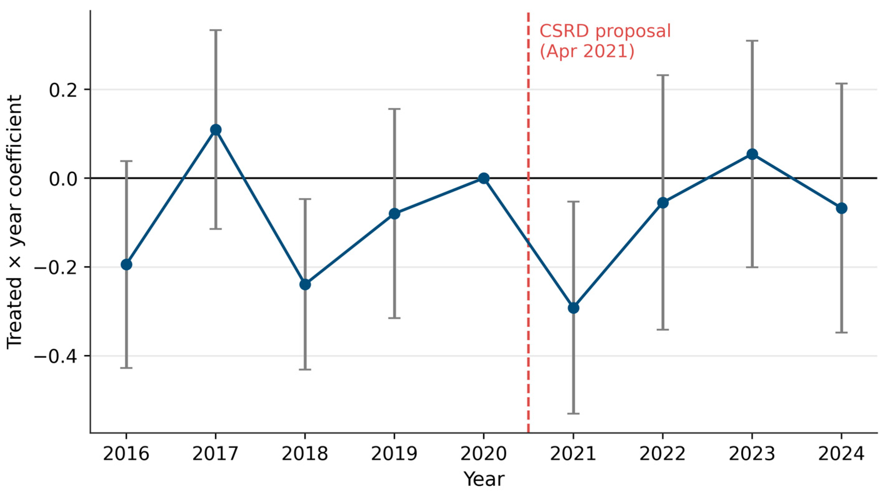
Design C tests parallel trends directly. On a panel spanning 2016 to 2024, we estimate treated-by-year interactions with firm and year fixed effects, normalised to 2020, the last complete year before the proposal, with standard errors clustered by firm. The pre-period coefficients are then jointly testable—the test the two-period design cannot support.

Design D is a daily event study. Abnormal returns are estimated from a market model over a 250-trading-day window ending 30 days before each event, using each firm’s own home market index as the market proxy. Because the common national market movement is removed by construction, this design is not exposed to the cross-country confounding that afflicts Design A. We cumulate abnormal returns over windows of one, three, five and 10 trading days either side of each of the five milestones and test the difference in mean cumulative abnormal return between in-scope and out-of-scope firms. Since this generates 20 tests, Bonferroni and Benjamini–Hochberg adjusted p-values are reported. Two further features of this design require attention. First, all firms share the same five event dates, so abnormal returns are cross-sectionally correlated within each group, and the conventional cross-sectional t-test overstates precision. We therefore report test statistics adjusted by the factor (1 + (n − 1) rho)^(1/2) of Kolari and Pynnönen (2010) across a range of average residual correlations rho, since rho cannot be estimated precisely from five event dates. Second, because our conclusion is a failure to reject, we do not treat a non-significant result as evidence of no effect. We conduct two one-sided tests of equivalence against a pre-specified bound of two percentage points, the order of magnitude of the announcement reactions reported for comparable disclosure mandates by Grewal et al. (2019), and we additionally report for each test the smallest bound at which equivalence would be established. This is what licences a statement about the range of effects the data exclude, in place of a statement that the effect is zero.

4. Results

4.1. Balance and Group Means

Table 3 reports balance on the matching covariates, on a common US-dollar basis. The correction matters for the first row. Converted at the 21 April 2021 spot rate of 1.2034, the treated mean is USD 47.78bn against USD 46.16bn for controls, a normalised difference of +0.042; comparing euro figures against dollar figures would instead indicate a difference of −0.181, which reflects the exchange rate rather than any difference in size. The groups are well balanced on size. Levered beta is likewise balanced at +0.084. Employees remain imbalanced at +0.307, treated firms being substantially larger. The final row is not a matching covariate and should not be read as a failure of the matching procedure, but it is the most consequential entry in the table: the 2021 pre-period return differs between the groups by more than one pooled standard deviation, so matching on sector, size, beta and market capitalisation did not produce groups whose returns behaved comparably. That anticipates the pre-trend rejection of Section 4.4.

Table 3. Pre-treatment balance on the matching variables.

Variable	Treated Mean	Control Mean	Normalised Difference	Variance Ratio	Balanced?
Market capitalisation (USD bn)	47.8	46.2	+0.042	1.22	yes
Employees	101,022	64,459	+0.307	2.31	no
Levered beta	1.047	1.016	+0.084	1.56	yes
Pre-period return (2021)	0.065	0.321	−1.009	0.66	no

Source: Authors’ calculations. Normalised differences above 0.25 in absolute value conventionally indicate imbalance. Market capitalisation is stated for both groups in US dollars, treated firms’ figures being converted from euro at the 21 April 2021 spot rate of 1.2034; comparing euro against dollar figures would yield a spurious normalised difference of −0.181 for that row. The pre-period return is not a matching covariate and is shown for comparison. Table 4 reports the realised within-pair matching distance, which balance in means does not capture.

Table 3. Pre-treatment balance on the matching variables.

Variable	Treated Mean	Control Mean	Normalised Difference	Variance Ratio	Balanced?
Market capitalisation (USD bn)	47.8	46.2	+0.042	1.22	yes
Employees	101,022	64,459	+0.307	2.31	no
Levered beta	1.047	1.016	+0.084	1.56	yes
Pre-period return (2021)	0.065	0.321	−1.009	0.66	no

Source: Authors’ calculations. Normalised differences above 0.25 in absolute value conventionally indicate imbalance. Market capitalisation is stated for both groups in US dollars, treated firms’ figures being converted from euro at the 21 April 2021 spot rate of 1.2034; comparing euro against dollar figures would yield a spurious normalised difference of −0.181 for that row. The pre-period return is not a matching covariate and is shown for comparison. Table 4 reports the realised within-pair matching distance, which balance in means does not capture.

Group-level balance is a limited diagnostic for a pair-matched design, since it may hold while individual pairs remain dissimilar. Table 4 therefore reports the realised distance within pairs, expressed in pooled standard deviations. The median absolute within-pair difference is 0.27 for market capitalisation and 0.18 for employees, but 0.72 for levered beta. The joint Euclidean distance across the three covariates has a median of 1.15, a 19th percentile of 2.03 and a maximum of 4.24, and 16 of the 40 pairs lie within one pooled standard deviation. The widest distances are recorded for Volkswagen and General Motors (4.24), Infineon and Texas Instruments (2.80), and Siemens and Eaton (2.60). The consequences for estimation are examined in Section 4.2.

Table 4. Realised within-pair matching distance, in pooled standard deviations.

Covariate	Median	Mean	90th Percentile	Maximum
Market capitalisation (USD)	0.265	0.388	0.905	2.075
Employees	0.180	0.444	0.764	4.156
Levered beta	0.718	0.889	1.740	2.412
Joint Euclidean distance	1.152	1.301	2.030	4.245

Source: Authors’ calculations. Each entry is the absolute difference between a treated firm and its matched control on the stated covariate, divided by the pooled standard deviation of that covariate across all 80 firms; the final row is the Euclidean norm of the three. Market capitalisation is converted to US dollars at the 21 April 2021 spot rate of 1.2034 before differencing. Sector is matched exactly for all 40 pairs. Sixteen of the 40 pairs lie within one pooled standard deviation on the joint measure and five within half of one. No caliper was imposed when the pairs were formed; Table 7 reports the effect of imposing one after the fact.

Table 4. Realised within-pair matching distance, in pooled standard deviations.

Covariate	Median	Mean	90th Percentile	Maximum
Market capitalisation (USD)	0.265	0.388	0.905	2.075
Employees	0.180	0.444	0.764	4.156
Levered beta	0.718	0.889	1.740	2.412
Joint Euclidean distance	1.152	1.301	2.030	4.245

Source: Authors’ calculations. Each entry is the absolute difference between a treated firm and its matched control on the stated covariate, divided by the pooled standard deviation of that covariate across all 80 firms; the final row is the Euclidean norm of the three. Market capitalisation is converted to US dollars at the 21 April 2021 spot rate of 1.2034 before differencing. Sector is matched exactly for all 40 pairs. Sixteen of the 40 pairs lie within one pooled standard deviation on the joint measure and five within half of one. No caliper was imposed when the pairs were formed; Table 7 reports the effect of imposing one after the fact.

Table 5 gives the four group-period means from which the difference-in-differences estimate is constructed, so that the estimate can be reconstructed by hand. Both groups earned markedly lower returns in 2022 than in 2021, this being a year of falling equity markets on both sides of the Atlantic, but the decline was smaller among treated firms. It is that difference in declines, 22.2 percentage points, which the estimator reports.

Table 5. Mean annual total returns (USD) by group and period.

	2021 (Pre)	2022 (Post)	Difference
Treated (in CSRD scope)	0.065	−0.135	−0.200
Control (out of scope)	0.322	−0.100	−0.422
Difference-in-differences			+0.222

Source: Authors’ calculations.

Table 5. Mean annual total returns (USD) by group and period.

	2021 (Pre)	2022 (Post)	Difference
Treated (in CSRD scope)	0.065	−0.135	−0.200
Control (out of scope)	0.322	−0.100	−0.422
Difference-in-differences			+0.222

Source: Authors’ calculations.

4.2. The Conventional Estimator

Table 6 reports the estimate across specifications. Two features stand out. The estimate is materially smaller, and no longer significant at conventional levels, when returns are measured in local currency, so roughly four percentage points of it reflect the differential depreciation of the euro rather than any difference in underlying performance. Furthermore, it is almost wholly insensitive to the control set, moving by less than two percentage points between the fully controlled specification and one with no firm-level controls at all, which suggests the accounting ratios contribute little.

Table 6. Difference-in-differences estimate across specifications.

Specification	n	Estimate	95% CI	p
Total return, USD (preferred)	153	+0.204	[0.041, 0.368]	0.015
Price return, USD	153	+0.194	[0.031, 0.356]	0.020
Total return, local currency	153	+0.167	[−0.003, 0.336]	0.054
Price return, local currency	153	+0.156	[−0.013, 0.325]	0.070
No firm-level controls	153	+0.222	[0.057, 0.388]	0.009
ROA only	153	+0.210	[0.046, 0.375]	0.013
Winsorised at 1%/99%	153	+0.189	[0.036, 0.341]	0.016

Source: Authors’ calculations.

Table 6. Difference-in-differences estimate across specifications.

Specification	n	Estimate	95% CI	p
Total return, USD (preferred)	153	+0.204	[0.041, 0.368]	0.015
Price return, USD	153	+0.194	[0.031, 0.356]	0.020
Total return, local currency	153	+0.167	[−0.003, 0.336]	0.054
Price return, local currency	153	+0.156	[−0.013, 0.325]	0.070
No firm-level controls	153	+0.222	[0.057, 0.388]	0.009
ROA only	153	+0.210	[0.046, 0.375]	0.013
Winsorised at 1%/99%	153	+0.189	[0.036, 0.341]	0.016

Source: Authors’ calculations.

Two sensitivity analyses address the construction of the control group. The first varies the composition of the matched sample; the second replaces pair matching with weighting. Both are reported in Table 7. Since no caliper was applied when the pairs were formed, one is applied ex post: pairs whose joint standardised distance in Table 4 exceeds a stated threshold are excluded and the specification re-estimated on the remainder. The estimate declines as the threshold tightens. At two pooled standard deviations it is +0.204 (n = 137, p = 0.022); at 1.5 standard deviations it falls to +0.123 and is no longer significant at conventional levels (n = 103, p = 0.235); at one standard deviation it is +0.046 (n = 63, p = 0.757). The estimate is therefore concentrated among the less comparable pairs and is not distinguishable from zero among the more comparable ones. A regulatory effect would not be expected to follow this pattern, since the Directive applies uniformly within the treated group irrespective of match quality. Residual heterogeneity between the two national samples is consistent with it.

Table 7. Sensitivity to control-pool composition and to weighting in place of pair matching.

Specification	n	Estimate	95% CI	p
Full matched sample (Table 6)	153	+0.204	[0.044, 0.365]	0.012
Caliper: pairs within 2.0 pooled SD	137	+0.204	[0.029, 0.379]	0.022
Caliper: pairs within 1.5 pooled SD	103	+0.123	[−0.080, 0.325]	0.235
Caliper: pairs within 1.0 pooled SD	63	+0.046	[−0.245, 0.336]	0.757
Propensity score ATT weighting	152	+0.210	[0.032, 0.387]	0.021
Entropy balancing	152	+0.231	[0.045, 0.417]	0.015

Source: Authors’ calculations, HC1 standard errors, preferred specification throughout (total return in US dollars, five accounting controls as z-scores). The caliper rows discard matched pairs whose joint standardised distance in Table 4 exceeds the stated threshold and re-estimate on the remainder. The propensity score is estimated by logit on log market capitalisation, log employees and levered beta, with average treatment effect on the treated weights of e/(1 − e) applied to controls. Entropy balancing reweights controls so that the means of those three covariates equal the treated means exactly; the resulting reweighted control means reproduce the treated means to three decimal places on all three covariates.

Table 7. Sensitivity to control-pool composition and to weighting in place of pair matching.

Specification	n	Estimate	95% CI	p
Full matched sample (Table 6)	153	+0.204	[0.044, 0.365]	0.012
Caliper: pairs within 2.0 pooled SD	137	+0.204	[0.029, 0.379]	0.022
Caliper: pairs within 1.5 pooled SD	103	+0.123	[−0.080, 0.325]	0.235
Caliper: pairs within 1.0 pooled SD	63	+0.046	[−0.245, 0.336]	0.757
Propensity score ATT weighting	152	+0.210	[0.032, 0.387]	0.021
Entropy balancing	152	+0.231	[0.045, 0.417]	0.015

Source: Authors’ calculations, HC1 standard errors, preferred specification throughout (total return in US dollars, five accounting controls as z-scores). The caliper rows discard matched pairs whose joint standardised distance in Table 4 exceeds the stated threshold and re-estimate on the remainder. The propensity score is estimated by logit on log market capitalisation, log employees and levered beta, with average treatment effect on the treated weights of e/(1 − e) applied to controls. Entropy balancing reweights controls so that the means of those three covariates equal the treated means exactly; the resulting reweighted control means reproduce the treated means to three decimal places on all three covariates.

The weighting estimators yield a different result. Propensity score weighting on log market capitalisation, log employees and levered beta gives +0.210 (p = 0.021); entropy balancing, which reweights the control group so that the means of these three covariates equal those of the treated group, gives +0.231 (p = 0.015). Neither departs materially from the baseline estimate. The divergence between the two exercises reflects the constraint each imposes. Weighting equalises covariate means across the two groups without altering the comparability of individual firms, whereas the caliper restricts the sample to firms that are similar pairwise. That the estimate is sensitive to the second constraint and not to the first is consistent with confounding at the level of the individual comparison rather than with a treatment effect.

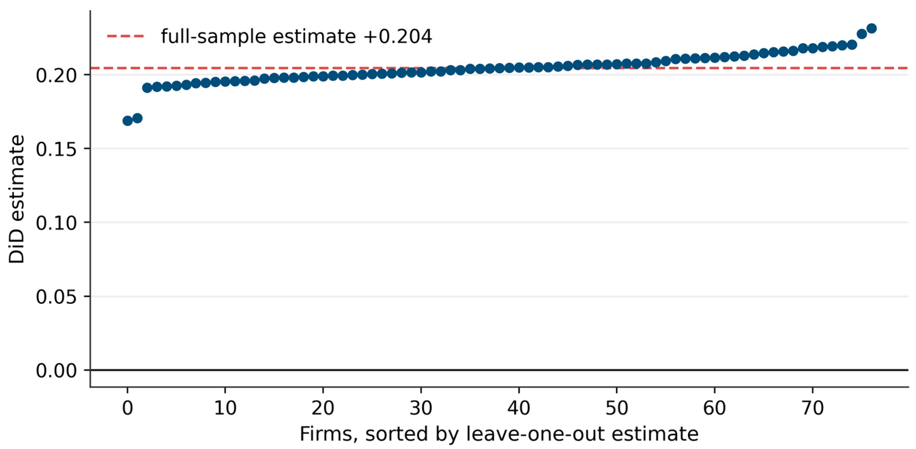
Table 8 shows that the estimate is equally insensitive to the method of inference. Leave-one-out estimation, dropping each firm in turn, confines it to the interval [0.169, 0.232], with a standard deviation across the 80 estimates of 0.010. By every criterion this literature conventionally applies—that is, robust and clustered standard errors, bootstrap methods, permutation distributions, winsorisation, control set sensitivity, and influence diagnostics—the estimate is stable. Stability is what all these criteria establish, and each of them conditions on firms being the relevant sampling units when treatment was in fact assigned to countries. The entries in Table 8 are accordingly reported as conditional firm-sampling diagnostics and not as tests of a policy effect. The remainder of this section establishes that the coefficient they describe is uninformative about the regulation.

Table 8. Inference on the preferred specification.

Method	Estimate	SE	95% CI	p
Conventional OLS	+0.204	0.083	[0.041, 0.368]	0.015
HC1 heteroskedasticity-consistent	+0.204	0.082	[0.044, 0.365]	0.012
Firm-clustered	+0.204	0.087	[0.034, 0.374]	0.018
Wild cluster bootstrap-t (4999 reps)	+0.204	—	—	0.019
Randomisation inference (4999 perms)	+0.204	—	—	0.021

Source: Authors’ calculations. n = 153 firm-years on 80 firms in two countries. The firm-clustered standard errors and the wild cluster bootstrap-t both cluster at the firm level, G = 80, with mean cluster size 1.9 (minimum 1, maximum 2). The bootstrap is a wild cluster bootstrap-t with Rademacher weights and the null imposed, 4999 replications, resampling at the firm level, with the p-value computed from the symmetric distribution of the studentised statistic. The permutation distribution reassigns the treated label across the 80 firms over 4999 draws, holding the number of treated firms fixed. None of these is inference at the level at which treatment was assigned. Treatment is assigned at the country level, giving G = 2, at which cluster-robust and wild-bootstrap procedures have no asymptotic justification and a permutation distribution admits at most two distinct assignments. The quantities reported here are therefore conditional firm-sampling diagnostics describing the stability of the coefficient under resampling of firms; they are not p-values for a policy effect and should not be read as such.

Table 8. Inference on the preferred specification.

Method	Estimate	SE	95% CI	p
Conventional OLS	+0.204	0.083	[0.041, 0.368]	0.015
HC1 heteroskedasticity-consistent	+0.204	0.082	[0.044, 0.365]	0.012
Firm-clustered	+0.204	0.087	[0.034, 0.374]	0.018
Wild cluster bootstrap-t (4999 reps)	+0.204	—	—	0.019
Randomisation inference (4999 perms)	+0.204	—	—	0.021

Source: Authors’ calculations. n = 153 firm-years on 80 firms in two countries. The firm-clustered standard errors and the wild cluster bootstrap-t both cluster at the firm level, G = 80, with mean cluster size 1.9 (minimum 1, maximum 2). The bootstrap is a wild cluster bootstrap-t with Rademacher weights and the null imposed, 4999 replications, resampling at the firm level, with the p-value computed from the symmetric distribution of the studentised statistic. The permutation distribution reassigns the treated label across the 80 firms over 4999 draws, holding the number of treated firms fixed. None of these is inference at the level at which treatment was assigned. Treatment is assigned at the country level, giving G = 2, at which cluster-robust and wild-bootstrap procedures have no asymptotic justification and a permutation distribution admits at most two distinct assignments. The quantities reported here are therefore conditional firm-sampling diagnostics describing the stability of the coefficient under resampling of firms; they are not p-values for a policy effect and should not be read as such.

4.3. Estimates from Event-Free Periods

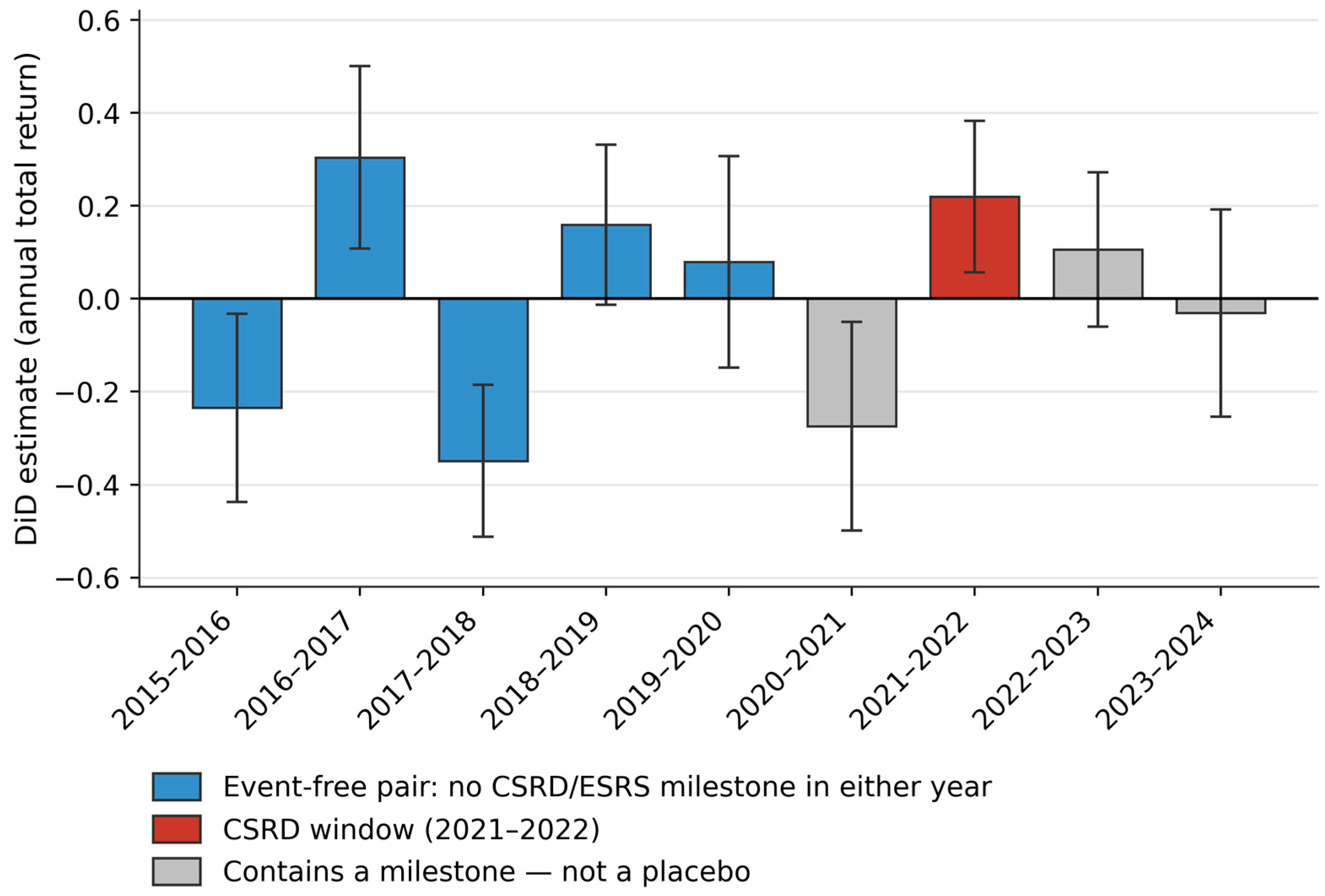
Table 9 and Figure 1 report Design B. Each of the nine adjacent year pairs is classified against the full five-event chronology of Table 1. Only five pairs, 2015–2016 through 2019–2020, contain none of the five milestones in either of their two calendar years. The four remaining pairs each contain at least one event and are not placebos; they are shown for completeness but excluded from the summary statistics.

Table 9. The identical design applied to every adjacent year pair.

Year Pair and Event Classification	n	Estimate	95% CI	p
2015–2016—event-free	144	−0.235	[−0.437, −0.032]	0.023
2016–2017—event-free	148	+0.304	[0.108, 0.501]	0.002
2017–2018—event-free	148	−0.349	[−0.512, −0.186]	<0.001
2018–2019—event-free	148	+0.160	[−0.013, 0.332]	0.069
2019–2020—event-free	150	+0.079	[−0.148, 0.307]	0.495
2020–2021—contains proposal (21 April 2021)	152	−0.274	[−0.498, −0.050]	0.017
2021–2022 (CSRD)—contains 2022 milestones; baseline year contains the proposal	154	+0.220	[0.057, 0.383]	0.008
2022–2023—contains 2022 milestones and ESRS (31 July 2023)	156	+0.106	[−0.060, 0.272]	0.211
2023–2024—contains ESRS (31 July 2023)	158	−0.031	[−0.253, 0.192]	0.788

Source: Authors’ calculations, HC1 standard errors. A pair is classified event-free only if neither of its calendar years contains any of the five milestones of Table 1. Across the five event-free pairs, the mean absolute estimate is 0.225, the standard deviation of the estimates is 0.274, the range is [−0.349, +0.304], and three of the five are significant at the 5% level. No empirical p-value is reported: five event-free comparisons cannot support one, and the design does not identify the null distribution that such a p-value would require. The four event-containing pairs, including the CSRD window itself, are shown for completeness only.

Table 9. The identical design applied to every adjacent year pair.

Year Pair and Event Classification	n	Estimate	95% CI	p
2015–2016—event-free	144	−0.235	[−0.437, −0.032]	0.023
2016–2017—event-free	148	+0.304	[0.108, 0.501]	0.002
2017–2018—event-free	148	−0.349	[−0.512, −0.186]	<0.001
2018–2019—event-free	148	+0.160	[−0.013, 0.332]	0.069
2019–2020—event-free	150	+0.079	[−0.148, 0.307]	0.495
2020–2021—contains proposal (21 April 2021)	152	−0.274	[−0.498, −0.050]	0.017
2021–2022 (CSRD)—contains 2022 milestones; baseline year contains the proposal	154	+0.220	[0.057, 0.383]	0.008
2022–2023—contains 2022 milestones and ESRS (31 July 2023)	156	+0.106	[−0.060, 0.272]	0.211
2023–2024—contains ESRS (31 July 2023)	158	−0.031	[−0.253, 0.192]	0.788

Source: Authors’ calculations, HC1 standard errors. A pair is classified event-free only if neither of its calendar years contains any of the five milestones of Table 1. Across the five event-free pairs, the mean absolute estimate is 0.225, the standard deviation of the estimates is 0.274, the range is [−0.349, +0.304], and three of the five are significant at the 5% level. No empirical p-value is reported: five event-free comparisons cannot support one, and the design does not identify the null distribution that such a p-value would require. The four event-containing pairs, including the CSRD window itself, are shown for completeness only.

The comparison is descriptive but stark. Across the five pairs in which no CSRD or ESRS event occurred, the identical design returns a mean absolute estimate of 0.225, which is larger than the 0.220 it returns in the CSRD window, with a standard deviation of 0.274 and a range from −0.349 to +0.304. Three of the five are significant at the 5% level, and three exceed the CSRD window estimate in absolute value. Restricting attention to genuinely event-free pairs, as the classification requires, strengthens this pattern: treating event-containing pairs as placebos understates the dispersion of the estimator in periods without regulatory news.

The evidence is descriptive rather than a formal test, and is sufficient for the present purpose. A two-period comparison of German and American annual returns generates estimates of 20 to 35 percentage points, of both signs and frequently significant, in years in which no event of regulatory relevance occurred. The dispersion of that differential is of the same order as the CSRD window estimate, which therefore cannot be distinguished from an ordinary draw from it. H3 is not supported. A further consideration compounds this: the 2021–2022 window is not a clean pre–post comparison, because the April 2021 proposal falls inside its baseline year.

4.4. Parallel Trends

Figure 2 plots the treated-by-year coefficients from Design C, normalised to 2020. The joint test of the four pre-period coefficients rejects parallel trends decisively, with F = 4.879 and p = 0.0015; the 2018 coefficient alone is −0.239. Treated and control returns did not move together before the CSRD, so the assumption on which any difference-in-differences interpretation depends does not hold in this sample. This is independent confirmation of the event-free-period evidence of Section 4.3, and it is the test the two-period design was unable to perform. One qualification carries over from Section 3.4: the pre-period coefficients are estimated with firm-clustered standard errors, which are conditional firm-sampling quantities rather than design-based ones, so the joint test should be read as strong descriptive evidence that the two series did not move together rather than as a formal test at the level of treatment assignment.

4.5. The Event Study

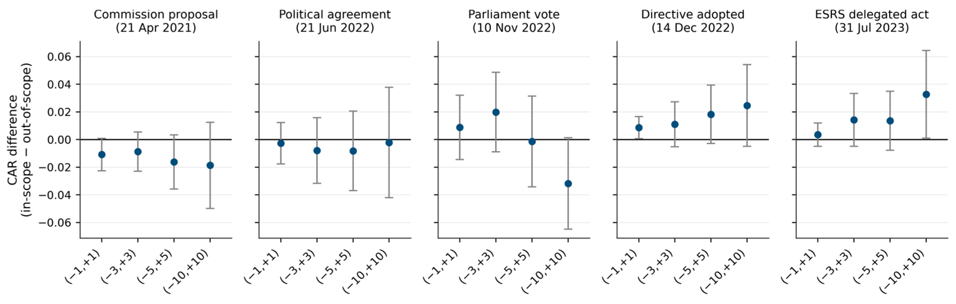
Design D is not exposed to the cross-country comparison, since abnormal returns are measured against each firm’s own home market index. Table 10 reports the difference in mean cumulative abnormal return at each milestone, with unadjusted and both sets of adjusted p-values reported in full. Two of the 20 tests have unadjusted p-values below 0.05, against one expected by chance under the null, and neither survives multiplicity control: the smallest Bonferroni-adjusted p-value is 0.728, and the smallest Benjamini–Hochberg-adjusted p-value is 0.310.

Table 10. Difference in cumulative abnormal returns, in-scope minus out-of-scope.

Event	(−1, +1) Diff (p) [Bonf; BH]	(−3, +3) Diff (p) [Bonf; BH]	(−5, +5) Diff (p) [Bonf; BH]	(−10, +10) Diff (p) [Bonf; BH]
Commission proposal, 21 April 2021	−0.011 (0.074) [1.000; 0.310]	−0.009 (0.230) [1.000; 0.376]	−0.016 (0.109) [1.000; 0.310]	−0.019 (0.245) [1.000; 0.376]
Political agreement, 21 June 2022	−0.003 (0.725) [1.000; 0.805]	−0.008 (0.516) [1.000; 0.645]	−0.008 (0.578) [1.000; 0.680]	−0.002 (0.916) [1.000; 0.934]
Parliament vote, 10 November 2022	+0.009 (0.458) [1.000; 0.611]	+0.020 (0.179) [1.000; 0.375]	−0.001 (0.934) [1.000; 0.934]	−0.032 (0.063) [1.000; 0.310]
Directive adopted, 14 December 2022	+0.009 (0.036) [0.728; 0.310]	+0.011 (0.188) [1.000; 0.375]	+0.018 (0.094) [1.000; 0.310]	+0.025 (0.106) [1.000; 0.310]
ESRS delegated act, 31 July 2023	+0.003 (0.418) [1.000; 0.598]	+0.014 (0.150) [1.000; 0.375]	+0.014 (0.216) [1.000; 0.376]	+0.033 (0.047) [0.934; 0.310]

Source: Authors’ calculations. Each cell reports the difference in mean cumulative abnormal return, with the unadjusted p-value in parentheses and the Bonferroni- and Benjamini–Hochberg-adjusted p-values in square brackets, in that order, computed over the family of 20 tests. Two tests have unadjusted p < 0.05, against 1.0 expected by chance under the null. No test survives either correction: the smallest Bonferroni-adjusted p-value is 0.728, and the smallest Benjamini–Hochberg-adjusted p-value is 0.310. All p-values in this table assume cross-sectional independence of abnormal returns. Because the five event dates are common to all firms, that assumption is not tenable, and Table 11 reports the consequences of relaxing it together with the corresponding equivalence bounds.

Table 10. Difference in cumulative abnormal returns, in-scope minus out-of-scope.

Event	(−1, +1) Diff (p) [Bonf; BH]	(−3, +3) Diff (p) [Bonf; BH]	(−5, +5) Diff (p) [Bonf; BH]	(−10, +10) Diff (p) [Bonf; BH]
Commission proposal, 21 April 2021	−0.011 (0.074) [1.000; 0.310]	−0.009 (0.230) [1.000; 0.376]	−0.016 (0.109) [1.000; 0.310]	−0.019 (0.245) [1.000; 0.376]
Political agreement, 21 June 2022	−0.003 (0.725) [1.000; 0.805]	−0.008 (0.516) [1.000; 0.645]	−0.008 (0.578) [1.000; 0.680]	−0.002 (0.916) [1.000; 0.934]
Parliament vote, 10 November 2022	+0.009 (0.458) [1.000; 0.611]	+0.020 (0.179) [1.000; 0.375]	−0.001 (0.934) [1.000; 0.934]	−0.032 (0.063) [1.000; 0.310]
Directive adopted, 14 December 2022	+0.009 (0.036) [0.728; 0.310]	+0.011 (0.188) [1.000; 0.375]	+0.018 (0.094) [1.000; 0.310]	+0.025 (0.106) [1.000; 0.310]
ESRS delegated act, 31 July 2023	+0.003 (0.418) [1.000; 0.598]	+0.014 (0.150) [1.000; 0.375]	+0.014 (0.216) [1.000; 0.376]	+0.033 (0.047) [0.934; 0.310]

Source: Authors’ calculations. Each cell reports the difference in mean cumulative abnormal return, with the unadjusted p-value in parentheses and the Bonferroni- and Benjamini–Hochberg-adjusted p-values in square brackets, in that order, computed over the family of 20 tests. Two tests have unadjusted p < 0.05, against 1.0 expected by chance under the null. No test survives either correction: the smallest Bonferroni-adjusted p-value is 0.728, and the smallest Benjamini–Hochberg-adjusted p-value is 0.310. All p-values in this table assume cross-sectional independence of abnormal returns. Because the five event dates are common to all firms, that assumption is not tenable, and Table 11 reports the consequences of relaxing it together with the corresponding equivalence bounds.

Two features deserve emphasis, and a third qualification limits both. There is no reaction surviving multiplicity control at any milestone. The estimated reaction to the proposal itself is negative in all four windows, reaching at most −1.9 percentage points, so whatever the annual estimator captures, it is not a positive repricing of exposed firms at the moment the mandate was proposed. The qualification is that these tests treat abnormal returns as cross-sectionally independent, and they are not: all firms share the same five event dates, and the residual correlation induced by common industry and factor exposure inflates the apparent precision of a cross-sectional t-test. Table 11 applies the Kolari-Pynnoenen adjustment across a range of average residual correlations. At rho = 0.02, a modest value for large firms within two countries, the standard errors rise by a factor of 1.32, and neither of the two nominally significant results remains significant even before multiplicity control. Cross-sectional dependence therefore reinforces the failure to reject while simultaneously widening the range of effects the design cannot exclude.

Table 11. Sensitivity of the event study inference to cross-sectional dependence, with the corresponding equivalence bounds.

Assumed Average Residual Correlation	SE Inflation Factor	Tests with Unadjusted p < 0.05 (of 20)	Smallest Unadjusted p-Value	Equivalence Bound Across All 20 Tests (pp)
0.00 (independence)	1.00	2	0.036	5.99
0.02	1.32	0	0.111	6.90
0.05	1.70	0	0.213	7.94
0.10	2.18	0	0.331	9.30

Source: Authors’ calculations. Standard errors are inflated by the Kolari–Pynnoenen factor (1 + (n − 1) rho)^(1/2), applied within each group, where rho is the assumed average pairwise correlation of market model residuals across firms on the common event dates. The equivalence bound is the smallest symmetric bound around zero at which two one-sided tests reject non-equivalence at the 5% level simultaneously for all 20 tests; restricted to the (−1, +1) and (−3, +3) windows, the corresponding bound is 4.43 pp at rho = 0. Because rho cannot be estimated precisely from five event dates, a range is reported rather than a single adjusted specification.

Table 11. Sensitivity of the event study inference to cross-sectional dependence, with the corresponding equivalence bounds.

Assumed Average Residual Correlation	SE Inflation Factor	Tests with Unadjusted p < 0.05 (of 20)	Smallest Unadjusted p-Value	Equivalence Bound Across All 20 Tests (pp)
0.00 (independence)	1.00	2	0.036	5.99
0.02	1.32	0	0.111	6.90
0.05	1.70	0	0.213	7.94
0.10	2.18	0	0.331	9.30

Source: Authors’ calculations. Standard errors are inflated by the Kolari–Pynnoenen factor (1 + (n − 1) rho)^(1/2), applied within each group, where rho is the assumed average pairwise correlation of market model residuals across firms on the common event dates. The equivalence bound is the smallest symmetric bound around zero at which two one-sided tests reject non-equivalence at the 5% level simultaneously for all 20 tests; restricted to the (−1, +1) and (−3, +3) windows, the corresponding bound is 4.43 pp at rho = 0. Because rho cannot be estimated precisely from five event dates, a range is reported rather than a single adjusted specification.

Because the finding is a failure to reject, we test equivalence rather than assert a null. Against the pre-specified bound of two percentage points, equivalence is established in only three of the 20 tests, namely the 1-day windows at the political agreement, at the Directive’s adoption and at the ESRS delegated act. For the remaining 17, the data are consistent with average reactions larger than two percentage points. The smallest bound at which equivalence holds simultaneously across all 20 tests is 6.0 percentage points; restricting attention to the 1- and 3-day windows, where a market model event study is most reliable, it is 4.4 points. Allowing for cross-sectional dependence widens these bounds further, to 6.9 points at rho = 0.02 and 7.9 points at rho = 0.05. The resulting statement is bounded rather than categorical. Over short windows, the average incremental reaction of in-scope firms at these five milestones is unlikely to have exceeded four to eight percentage points in absolute value, the range depending on the correlation assumed; reactions below that magnitude cannot be distinguished from zero by this design.

The two designs can be compared directly. Summing the milestone estimates gives a cumulative 3-day reaction across the five events of +0.75 percentage points, with a standard error of 1.65 and a 95% confidence interval of [−2.47, +3.97]; the 7-day figure is +2.85 points, interval [−1.87, +7.57]. Allowing for cross-sectional dependence at rho = 0.05 widens the 3-day interval to [−4.73, +6.23] and the widest 21-day interval to [−12.18, +13.14]. The annual estimator’s +20.4 points lie outside all of these intervals. If the annual estimate reflected the Directive, a repricing of that order would have had to occur at the dates on which the mandate became public, and it did not. The two strategies are therefore not separately inconclusive but jointly informative: the daily evidence rejects the magnitude of the annual comparison reports (Figure 3).

4.6. Index Membership Against Regulatory Scope

Section 3.1 noted that 13 treated firms were not index constituents when the CSRD was proposed. This permits an internal falsification test, reported in Table 12. Restricting the treated group to genuine constituents raises the estimate to +0.243; restricting it to the firms admitted afterwards gives +0.107, indistinguishable from zero. Both subgroups are German, and both fall within CSRD scope under Article 19a, so a genuine regulatory effect ought to appear in both. That the estimate splits on index membership rather than on regulatory reach is difficult to reconcile with a regulatory interpretation and easy to reconcile with the estimator tracking the return behaviour of a particular set of large German equities.

Table 12. The estimate by definition of the treated group.

Treated Group	n	Estimate	95% CI	p
Full treated group	153	+0.204	[0.044, 0.365]	0.012
DAX constituents on 21 April 2021 only	130	+0.243	[0.089, 0.396]	0.002
Firms admitted to the DAX after the proposal	99	+0.107	[−0.205, 0.419]	0.501
Excluding negative book equity firm-years	136	+0.230	[0.065, 0.395]	0.006

Source: Authors’ calculations, HC1 standard errors. All subgroups are German, and all fall within CSRD scope under Article 19a.

Table 12. The estimate by definition of the treated group.

Treated Group	n	Estimate	95% CI	p
Full treated group	153	+0.204	[0.044, 0.365]	0.012
DAX constituents on 21 April 2021 only	130	+0.243	[0.089, 0.396]	0.002
Firms admitted to the DAX after the proposal	99	+0.107	[−0.205, 0.419]	0.501
Excluding negative book equity firm-years	136	+0.230	[0.065, 0.395]	0.006

Source: Authors’ calculations, HC1 standard errors. All subgroups are German, and all fall within CSRD scope under Article 19a.

4.7. What the Design Could and Could Not Have Detected

A final diagnostic concerns statistical power. At 80% power and the 5% level, the annual design has a minimum detectable effect of 23.1 percentage points, rising to 26.8 points at 90% power. Its own point estimate of 20.4 points lies below that threshold. An estimate falling below the minimum detectable effect is not thereby invalid: the minimum detectable effect is an ex-ante property of a design and carries no information about whether any particular realised estimate is correct. What the comparison does imply is a magnitude problem. When power is low, the estimates that clear the significance threshold are a selected subset, because only large draws clear it, so conditional on significance they overstate the truth and can invert its sign. For this design, the exaggeration is severe: against a true effect of two percentage points, a statistically significant estimate would on average overstate it by a factor of about 10 and would carry the wrong sign about a quarter of the time; against a true effect of five points the factor is about four and the sign error about one in 20. The significance of the +0.204 coefficient is therefore consistent with a wide range of underlying truths, including zero, and constitutes very weak evidence for any of them. The event study is far better placed but is not precise either: what it can exclude are the short-window equivalence bounds of roughly four to eight percentage points reported in Section 4.5.

Figure 4 is the methodologically instructive exhibit of the paper. It displays an estimate that is, by every conventional criterion, entirely stable: it survives every alteration of the specification, every method of inference, and the removal of any single firm. Section 4.3, Section 4.4, Section 4.5, Section 4.6 and Section 4.7 establish that it is nonetheless measuring a differential country shock rather than a regulatory effect. Influence diagnostics, robust inference and bootstrap methods establish whether an estimate is stable; they do not establish whether it identifies anything.

5. Discussion

5.1. What the Evidence Supports

An analysis that stopped at Table 8 would report a positive announcement effect of some 20 percentage points, supported by a robustness table of exactly the kind this literature routinely presents: significance under four methods of inference, insensitivity to the control set, stability under winsorisation, and no dependence on any individual firm.

The diagnostics of Section 4.3, Section 4.4, Section 4.5, Section 4.6 and Section 4.7 show that such a conclusion would have been mistaken. The design produces estimates of comparable magnitude and mixed sign in years containing no CSRD or ESRS event; the coefficient vanishes once the sample is restricted to well-matched pairs; parallel trends are formally rejected; the effect splits on index membership rather than on regulatory scope; the design is badly underpowered for effects of the size it reports; and the event study, which does not rely on the cross-country comparison, finds nothing that survives multiplicity control or the correction for cross-sectional dependence. We therefore conclude that these data provide no evidence that the CSRD proposal or its subsequent milestones produced a detectable incremental repricing of exposed firms, and that the conventional estimate which appears to show one is not informative about the regulation.

The strength of this conclusion requires qualification. It is a bounded failure to detect, not a demonstration that the effect is zero. The annual design is underpowered for effects of the size at issue and cannot be given a design-based interpretation in any case, since treatment is assigned to two jurisdictions. The event study, while far better placed, excludes average short-window reactions of roughly four percentage points and above under cross-sectional independence, and roughly eight points and above under plausible residual correlation; it cannot exclude smaller reactions. The two strategies are nonetheless jointly informative rather than separately inconclusive. The cumulative 3-day reaction across the five milestones, +0.75 percentage points with a confidence interval of [−2.47, +3.97], excludes the 20.4 points the annual estimator reports; a repricing of that magnitude did not occur in the announcement windows, which is what the annual estimate would require if it reflected the Directive. What the two designs establish together is that there is no evidence of a large incremental repricing at any milestone, and that the one estimate appearing to show a large effect cannot be distinguished from the ordinary year-to-year volatility of the German–American return differential.

5.2. Reconciling a Divided Literature

These findings bear directly on Boungou and Dufau (2025), who report European underperformance around CSRD and ESRS events. We do not claim their result is spurious. Their sample is larger by three orders of magnitude, they use daily rather than annual data, and short windows are far less exposed to the contamination documented here. But their identifying variation is also cross-country, and our placebo evidence shows that this source of variation is contaminated over precisely this period. The natural reconciliation is that the sign of a cross-country estimate in this window depends on the comparison set and the horizon—a proposition that is testable, since a placebo exercise on their design, using event dates drawn from periods without European regulatory news, would settle whether their estimate survives it.

The argument generalises. Section 2.3 described a literature that has been unable to agree on the sign of an effect across three waves of increasingly sophisticated designs, and attributed that disagreement to institutional heterogeneity. Our results suggest a substantial part of the dispersion may instead reflect the sampling distribution of the design itself: if cross-jurisdiction comparisons over annual horizons are centred on whatever the differential country shock happened to be, then positive findings for the United Kingdom and India, negative findings for China, and mixed findings within Europe are not necessarily statements about those jurisdictions. On this reading, the field’s inconsistency is partly a measurement artefact, and the appropriate response is design discipline rather than further accumulation of estimates. The placebo test we implement is inexpensive, requires no data beyond what such studies already assemble, and should in our view be routine.

5.3. The Limits of What a Sign Can Tell Us

Section 2.2 showed that the information-asymmetry and proprietary-cost channels predict opposite signs but the same cross-sectional concentration. It follows that inferring a mechanism from the sign of an average coefficient—reading a positive estimate as evidence of a disclosure-benefits channel—does not go through even when the coefficient is well identified. Distinguishing the channels requires relating the reaction to the incremental disclosure burden each firm faces. We were unable to construct such a measure from the data available, and rather than claim a mechanism we cannot identify, we set out in Section 6 the design that would be needed.

5.4. Limitations

Several limitations should be acknowledged. The most important concerns the strength of the null. Our event study can exclude average short-window reactions above roughly four percentage points under cross-sectional independence, and above roughly eight points once plausible residual correlation is allowed for; economically meaningful effects smaller than that cannot be excluded, and we make no claim about them. Second, and relatedly, the annual design cannot be given a design-based interpretation at all, because treatment is assigned to two jurisdictions; estimates from it are reported as descriptive decompositions of a country differential rather than as causal quantities. Third, the treated firms are large-capitalisation companies already reporting under the NFRD, for whom the incremental burden of the CSRD is smallest, which limits external validity to precisely the population in which the largest effects might be expected. Fourth, we make no claim about the direction in which the 2022 energy and war shocks bias the comparison: that direction cannot be signed without knowing the relative sectoral composition of the two groups, which is why we examine event-free periods rather than reason about it. Fifth, the matched pairs were formed without a caliper, and Table 4 shows the realised pairing is loose, with a median joint distance of 1.15 pooled standard deviations; we regard the caliper-restricted estimates of Table 7 as the more credible reading of the annual design rather than as a robustness check upon it. Sixth, treated and control accounting quantities are prepared under IFRS and US GAAP respectively and are not restated to a common basis, so the ratio controls should be read with that in mind. Those controls are also measured contemporaneously rather than at a fixed pre-treatment date, so, as Section 3.3 sets out, they are descriptive covariates rather than pre-treatment causal controls. Seventh, the control group contains firms with material EU exposure, three of them within Article 19a scope outright; we audit and correct for this in Section 3.1, but any residual undetected exposure would bias the comparison towards zero. Finally, this is a study of announcements. It speaks to how markets priced expectations, not to the realised consequences of the regime once ESRS reporting began.

6. Conclusions

We asked whether equity markets registered a discrete incremental reaction at the five dates on which the content of the European Union’s most far-reaching disclosure mandate became public. The conventional two-period difference-in-differences estimator returns +0.204, with a 95% confidence interval of [0.041, 0.368], and is stable under heteroskedasticity-consistent, clustered and bootstrap procedures and under leave-one-out estimation. We conclude that it does not identify a regulatory effect, and that its stability was never capable of showing that it did. Applied to the 5 year pairs that contain none of the five milestones, the same design yields estimates averaging 0.225 in absolute value, larger than the CSRD window estimate itself, with three of five significant at conventional levels; a caliper on the realised matching distance reduces the estimate from +0.204 to +0.046; parallel pre-trends are rejected; the design’s minimum detectable effect of 23.1 percentage points implies that any significant estimate it produces will substantially overstate the truth; the effect splits on index membership rather than on regulatory scope; and the daily event study finds no reaction surviving multiplicity control or the correction for cross-sectional dependence at any of the five CSRD and ESRS milestones, with the estimated reaction to the proposal itself small and negative. We report this as a bounded failure to detect rather than as a null: equivalence tests place the average short-window reaction within roughly four to eight percentage points in absolute value, depending on the correlation assumed, and smaller reactions remain possible.

The paper contributes to the literature on the capital market consequences of mandatory non-financial disclosure in three respects. It provides an assessment of a CSRD announcement effect that is validated against periods in which no such announcement occurred. It demonstrates that an estimate can satisfy every robustness check customary in this field while identifying nothing, because those checks examine stability rather than meaning. Furthermore, it offers a design-based account of the field’s inconsistency that can be tested on existing studies rather than merely asserted about them.

The practical implications are mainly cautionary, and we state them in proportion to the strength of the evidence. We find no evidence that anticipated compliance costs were capitalised, or that reporting readiness was rewarded, at any of the five milestones, and preparers should not plan on the basis that they will be; we cannot exclude reactions below the bounds our tests resolve. Investors should be slow to attribute return differences between European and American firms over 2021 and 2022 to the Directive, since differences of similar magnitude occurred in years containing no CSRD or ESRS event. Policymakers and standard-setters weighing the phased ESRS timetable and the current simplification proposals will find that market-based evidence from cross-country comparisons over this window is too weakly identified to support a conclusion in either direction, and arguments in that debate resting on such evidence should be treated with corresponding caution. We emphasise that this is a claim about the evidentiary value of a class of studies, including our own annual specification, and not a claim that mandatory sustainability reporting lacks a capital market rationale. Our design speaks to announcement windows; the premise on which the policy rests, concerns the regime in operation, which these data cannot address.

Five directions for further work follow from the analysis. The most valuable, in our judgement, is to disaggregate the three ESG pillars, since the ESRS impose markedly different incremental obligations on environmental, social and governance reporting—the environmental standards being considerably more prescriptive and quantitative—so that a composite treatment averages over heterogeneity that theory says should matter, and pillar-level measures would permit three independent tests in which disagreement would itself be informative. The second is to construct a firm-level measure of incremental disclosure burden and compare firms within a single country and currency, which would hold constant everything the placebo test shows to be confounding and would distinguish the disclosure-benefits from the proprietary-cost channel; the scope thresholds of Article 19a offer regression discontinuity variation that requires no matching at all. The third is to extend the outcome set beyond returns to the cost of equity and debt, bid-ask spreads and analyst forecast dispersion, which speak to the information-asymmetry channel more directly than prices and are less exposed to macroeconomic contamination. The fourth is to examine cross-industry variation, testing whether any reaction concentrates in sectors of high environmental materiality, where the two channels make their most divergent predictions. The fifth is to exploit the ESRS revision process and the 2025 simplification proposals as information events running in the opposite direction to the original mandate: under either channel, a loosening should reverse the sign of the reaction to the tightening, and the relative magnitudes would be informative about which channel dominates. A sixth direction follows from the identification problem itself. Because a disclosure mandate is assigned to a jurisdiction, credible design-based inference requires variation at that level: either several treated and several comparison jurisdictions, permitting clustering and placebo assignment at the level at which treatment was actually assigned, or a synthetic-control or generalised synthetic-control estimator in which a weighted combination of untreated jurisdictions reproduces the treated jurisdiction’s pre-treatment path and inference proceeds by permuting treatment across jurisdictions. The staggered transposition of the CSRD into national law, and the divergent timetables of non-EU regimes, offer exactly this variation. We regard building such a design as the natural successor to the present paper, and the diagnostics reported here as an argument for why it is necessary.