A Production Function-Based Financial Feasibility Model (PFFM) and Social Return Assessment of Public Electric Bus Investment: Evidence from Thailand

Abstract

Most public investment feasibility studies rely on the linear assumption model (LAM), which assumes constant growth in revenues and costs and may overlook the underlying production structure. This study develops a Production Function-Based Financial Feasibility Model (PFFM) by integrating a Cobb–Douglas production function into cash flow analysis. It also applies the model to a 15-year electric bus project operated by the Khon Kaen Provincial Administrative Organization, covering three routes and a total investment of THB 285.05 million. The analysis uses deterministic projections based on expert-validated growth assumptions. Ordinary least squares estimation yields an energy elasticity of 0.990; however, because energy consumption is derived from a fixed rate per kilometre, this coefficient primarily reflects the internal consistency of the projections rather than an independently estimated behavioural relationship. Returns to scale are statistically indistinguishable from unity (RTS = 1.006; p = 0.95). Based solely on farebox and advertising revenues, both the LAM and PFFM indicate that the project is financially infeasible, with base-case NPVs of −THB 271.74 million and −THB 271.61 million, respectively, B/C ratios of approximately 0.54, and unattainable IRRs. This conclusion remains unchanged under a 30% increase in electricity prices. Although the two models produce similar results because RTS is close to unity, the PFFM provides a more transparent decomposition of fixed and marginal costs and clearer diagnostic insights into production technology and cost risk. In addition, an SROI analysis covering environmental, health, safety, and time-saving benefits, together with net-impact adjustments, yields a ratio of 3.45, indicating that the project generates substantial social value despite its financial infeasibility. The proposed framework therefore provides public agencies with a more comprehensive basis for investment decisions, subsidy design, and public service obligation policies.

1. Introduction

The Khon Kaen Provincial Administrative Organization (Khon Kaen PAO) has adopted a policy to develop a public transportation project using electric buses (EV buses) in Mueang Khon Kaen District to improve public transportation, alleviate traffic congestion, support the Smart City agenda, and reduce greenhouse gas emissions, in line with Thailand’s 13th National Economic and Social Development Plan (Kongwee et al., 2025; Prapaporn et al., 2022). The transition from diesel buses to electric buses is an important strategy for reducing air pollution and promoting sustainable urban development, as EV buses produce indirect exhaust emissions and generate significantly lower noise levels than diesel buses (Pei et al., 2024). At the same time, public transport systems play an essential role in addressing environmental and traffic-related externalities, with government subsidies serving as an important policy instrument (Tantiwat, 2025). If fully developed across all three routes, the project would require an investment of more than 200 million Baht (Chantuk et al., 2026) and would have long-term implications for the public budget. Therefore, Khon Kaen PAO commissioned a comprehensive financial feasibility study to support investment decision-making.

The Khon Kaen EV Bus project was selected as the case study for three primary reasons. First, as the economic and educational hub of Northeastern Thailand, Khon Kaen faces severe traffic congestion and PM 2.5 pollution, with AQI reaching 99 in 2025, and 94% of residents rely on private vehicles due to inadequate public transport. Second, the project aligns with the Provincial Administrative Organization’s ‘9 Good’ policy framework, targeting the environment, education, and mobility, while supporting Thailand’s EV strategy and SDGs 11 and 13. Third, with a total investment exceeding THB 285 million across three major routes, the project delivers substantial public benefits, including free fares for vulnerable groups (students, the elderly, and persons with disabilities). Furthermore, it presents unique regulatory and contractual challenges, including route overlaps with existing operators, licensing procedures, and O&M contract design under public procurement laws, making it a compelling policy case study for other local governments in Thailand and developing countries.

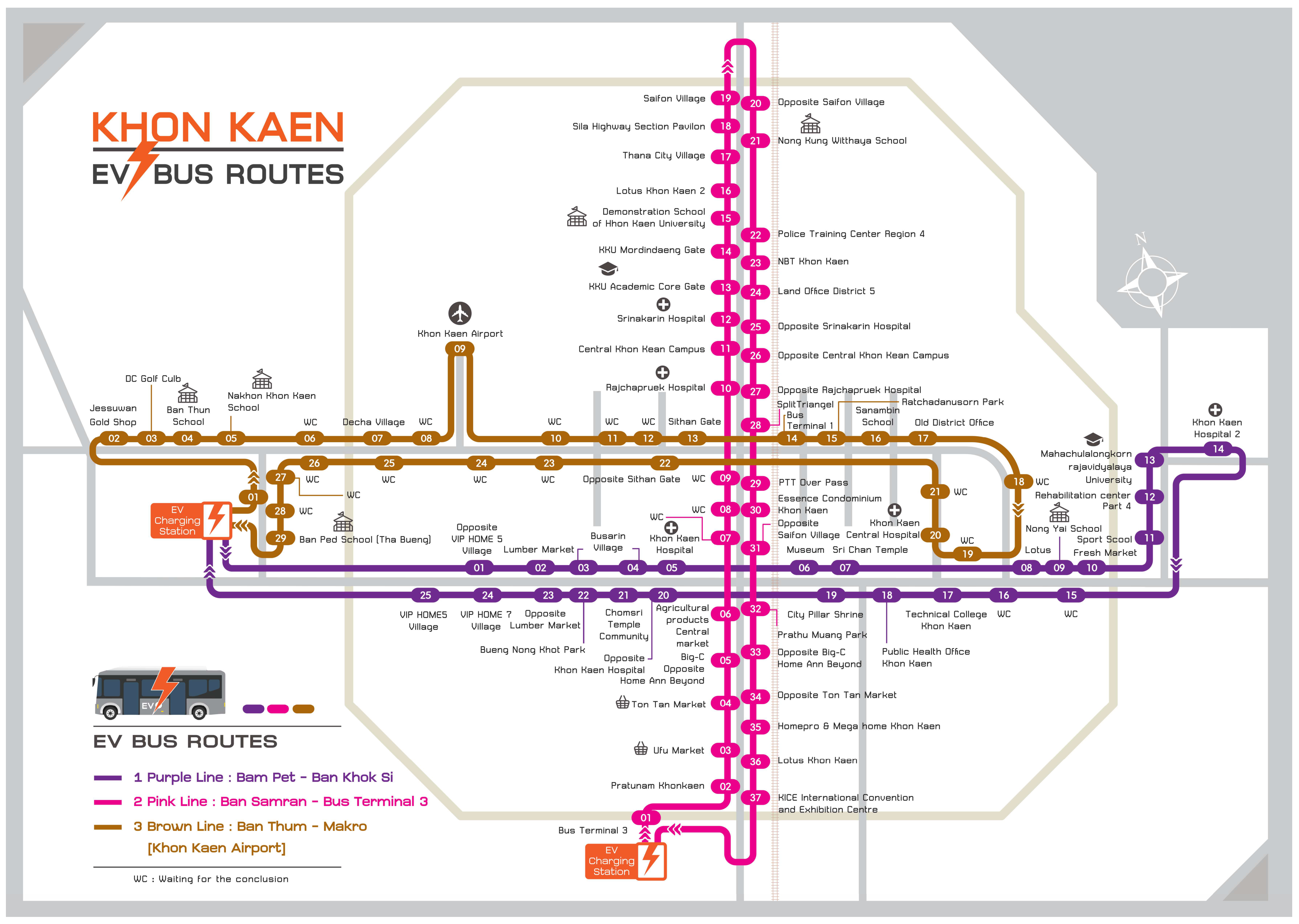
As shown in Figure 1, three EV bus routes are proposed for Mueang Khon Kaen District. These routes were designed based on passenger demand surveys, population density analysis, and connectivity with existing transport hubs, including the bus terminal, Khon Kaen University, the airport, and major commercial areas. The three routes serve distinct but complementary functions within the city’s public transportation network.

Financial feasibility studies of public investment projects generally rely on the linear assumption model (LAM), which assumes that revenues increase at a constant rate, such as 3% per year, while operating costs vary with service distance under a fixed-unit-cost assumption (Shim & Kim, 2022). Although this approach is simple and widely used, it has important structural limitations. Specifically, LAM does not explicitly incorporate the project’s underlying production structure when formulating financial assumptions. It therefore does not provide an explicit mechanism for estimating how production inputs, such as energy, labour, and capital, are related to output—in this case, the vehicle-kilometres of service operated—or for quantifying the contribution of each input to projected output (Muhamed et al., 2023; Walters, 1963). These limitations may affect the accuracy of cost estimates, expenditure assumptions, and project risk assessments.

While Asian economies such as China, South Korea, and Japan have made significant progress in developing and studying electric bus public transportation systems (Wang et al., 2024; Kim et al., 2021; Land Transport Authority, 2023), prior studies in this region have focused primarily on engineering and operational dimensions, such as cross-line dispatching optimisation, charging infrastructure planning, and fleet management. The reviewed literature provides limited evidence of the systematic integration of production function parameters into financial feasibility analysis.

In the Thai context, Chiradjea et al. (2025) conducted a financial feasibility study of EV charging infrastructure in high-density residential buildings, employing financial tools such as NPV, IRR, payback period, and sensitivity analysis. Their findings revealed that pricing strategy is the most critical determinant of project viability: break-even is attainable only at a profit margin of 8 THB per kWh, and a 10% reduction in either profit share or utilisation rate eliminates the project’s ability to reach payback. However, their study did not integrate production function parameters, such as returns to scale and marginal cost, into the financial modelling framework, a gap that our study seeks to address.

Furthermore, Gómez-Restrepo et al. (2024) conducted a scientometric analysis of 268 studies on financial valuation methods for photovoltaic projects with energy storage systems. Their analysis revealed that traditional methods, particularly levelised cost of energy (LCOE), net present value (NPV), and internal rate of return (IRR), remain the most widely used approaches. In contrast, advanced methods such as real options have been applied in only a limited number of studies. More importantly, the reviewed studies did not integrate production function parameters into financial analysis, highlighting a methodological gap that the present study addresses in the public transportation sector.

A review of the financial feasibility report for the Khon Kaen PAO EV Bus project, together with related studies conducted in Thailand (Saelee, 2021; Chantuk et al., 2026) and internationally (Cartenì, 2018; Wang et al., 2024), further indicates that production functions have not been systematically used to link financial assumptions with the underlying production technology of public transport projects. Consequently, revenue and expenditure assumptions generally remain linear and may not adequately reflect the project’s cost structure (Massot, 2014; Terblanche & Root, 2022), potentially reducing the accuracy of financial feasibility and risk assessments.

Beyond financial viability, public EV bus projects may generate substantial social and environmental value that is not captured by farebox revenue or conventional discounted cash flow indicators. Relevant outcomes may include improved mobility and accessibility for students, older persons, persons with disabilities, and low-income passengers; reduced transport-related social exclusion; lower greenhouse gas emissions and local air pollution; reduced noise; and associated public health benefits. Previous research on bus electrification has similarly distinguished financial and operational costs from broader environmental, health, and social outcomes when assessing project value (Vijay et al., 2023).

To address the identified financial appraisal gap, this study develops a Production Function-Based Financial Feasibility Model (PFFM) by systematically integrating the Cobb–Douglas production function into a discounted cash flow analysis framework. Rather than relying exclusively on linear revenue and cost assumptions, the proposed model incorporates production-related parameters to provide a more transparent and verifiable appraisal framework for public investment projects characterised by high fixed costs and technology-dependent operating structures.

The study distinguishes financial feasibility from broader public value while recognising that both dimensions are necessary for appraising public EV bus projects. The PFFM is designed to improve the estimation of production-related output, revenues, operating costs, and project cash flows; however, it does not independently measure social value. The financial results generated by the PFFM are therefore considered alongside a social return on investment (SROI) assessment, which captures accessibility, environmental, health, and distributional outcomes that are not reflected in farebox revenues or conventional financial indicators (Nicholls et al., 2012; Corvo et al., 2022).

The combined application of PFFM and SROI enables decision-makers to distinguish financial feasibility from broader public value. While PFFM provides transparent estimates of production costs and financial performance, SROI monetises relevant social and environmental outcomes. Together, they offer a more comprehensive framework for assessing whether a project’s wider public benefits are proportionate to the required public expenditure.

2. Literature Review

To ensure that the development of the conceptual framework for the Production Function-Based Financial Feasibility Model (PFFM) is grounded in both theoretical foundations and empirical evidence, the researchers conducted a systematic review of the literature by dividing them into four main dimensions: (1) the evolution of production functions and cost functions; (2) the application of production functions in investment and project analysis; (3) investment dynamics and financial constraints; (4) financial feasibility and policy implications; (5) financial feasibility studies of energy and transportation infrastructure in Thailand; (6) scientometric review of financial valuation methods; and (7) research conceptual framework and hypothesis framework.

2.1. The Evolution of Production Functions and Cost Functions

Cobb and Douglas (1928) introduced the power-form production function, which subsequently became a fundamental basis of modern production economics. This function effectively explains the relationship between output and key production inputs (Gordon & Vaughan, 2011). Based on empirical evidence, Walters (1963) concluded that the cost structures of public transportation and utility enterprises are complex and non-linear. This is consistent with recent studies on cost estimation, which indicate that traditional techniques, such as unit-rate or parametric estimation methods, often fail to capture market volatility and structural uncertainty, leading to inaccurate estimates (Blessing & Ifeanyi, 2025). Furthermore, Booth (1991) noted that production technologies with low substitutability among inputs, or fixed technology, expose enterprises to higher risks arising from changes in input prices. This mechanism is a key feature of the PFFM, which detects risks often overlooked by linear assumption models. The model employs the Cobb–Douglas production function, which is rooted in the seminal work of Cobb and Douglas (1928). However, the study by Felipe and Adams (2005) indicated that parameter estimation must carefully consider the structural relationships among production inputs. Furthermore, from the perspectives of macroeconomics and finance, Benchimol (2015) observed that money may be an overlooked production input in traditional models. The study proposed that financial liquidity plays a crucial role in production efficiency and enterprise risk, even though its weight in the physical production process may be relatively small. However, neglecting this financial dimension may lead to inaccurate risk assessment, which is inconsistent with the PFFM’s underlying objective of systematically integrating economic and financial parameters.

In the context of latent capital measurement and depreciation, Boratyński and Osiewalski (2021) and Boratyński and Osiewalski (2021) proposed a Bayesian estimation framework for capital stock and depreciation rates under data constraints. Their studies indicate that traditional accounting data often distort actual production capacity because they do not reflect efficiency decay. This is particularly relevant for high-technology assets, such as electric batteries. Meanwhile, Stadtherr and Wouters (2021) extended the scope of cost management beyond variable production costs to include portfolio-level management of R&D and infrastructure costs, reflecting the need for modern project appraisal to consider full life-cycle costing rather than focusing solely on annual operating costs.

2.2. The Application of Production Functions in Investment and Project Analysis

Several studies have applied production functions to project appraisal and investment analysis. Koval et al. (2018) confirmed that the Allen production function can be used to forecast output and assess investment efficiency. Meanwhile, Karimova (2026) noted that investment efficiency depends not only on the amount of capital invested but also on the direction of investment and the underlying production technology. Similarly, Rezepin et al. (2017) applied the Cobb–Douglas production function to analyse the production processes of industrial enterprises, emphasising that estimating the elasticity of revenue with respect to production inputs, such as capital and labour, using actual financial data can help identify the direction of technological change that generates the highest returns and serves as an important basis for formulating effective investment strategies. Dai and Zhou (2011) were among the early scholars to apply the Cobb–Douglas production function to the feasibility study of industrial funds. Massot (2014) proposed a long-term project appraisal framework that emphasised the use of an explicit production function rather than a conventional logistic function. This approach is consistent with the PFFM, which directly uses production parameters to formulate cash flow assumptions. Similarly, Fahrizal et al. (2020) developed a production optimisation model integrated with financial feasibility analysis for industrial applications. Their study indicated that formulating revenue and cost assumptions based on actual resource constraints and production technology can reduce errors in project viability assessments compared with traditional linear assumption approaches. This approach supports the PFFM concept, which aims to eliminate systematic bias by integrating production parameters into the financial analysis process in a structured manner.

In the context of Thailand’s service sector, Chantuk (2016) applied marginal cost (MC) and marginal revenue (MR) analysis to identify the profit-maximising and break-even points for a boutique hotel project. The study demonstrated that analysing cost structures in relation to production levels can effectively support decision-making on the appropriate scale of investment and on the attainment of economies of scale (Chantuk, 2016). However, the study relied on linear assumptions and polynomial functions for estimation, which did not sufficiently reflect the underlying mechanisms of input substitution. Therefore, the PFFM extends this approach by directly deriving MC and RTS parameters, enabling a more accurate and consistent investment-viability assessment than traditional models using actual production technology.

In the practice of engineering economics, Hasugian et al. (2020) demonstrated that break-even point (BEP) analysis, fixed and variable cost structures, and financial indicators such as NPV, IRR, and B/C ratio remain central to investment decision-making in the industrial and SME sectors. However, the revenue and cost estimations in these studies still rely on a constant growth rate. Therefore, the PFFM extends these approaches by replacing such assumptions with parameters that can be empirically estimated from data (RTS). This approach is consistent with recommendations to apply hybrid estimation and probabilistic modelling to reduce optimism bias in budgeting (Blessing & Ifeanyi, 2025).

2.3. Investment Dynamics and Financial Constraints

Studies on modern investment dynamics indicate that investment decisions are inseparable from financial constraints and production structures. Ikonnikova et al. (2022) developed a model showing that production capacity constraints and future price expectations strongly influence investment under uncertainty. This is consistent with the context of electric buses, which are exposed to energy-price volatility and labour capacity constraints. In addition, empirical research by Albulescu (2020) indicated that firms’ investment behaviour is not determined solely by external factors, but is also shaped by internal financial performance, particularly liquidity and profitability. These factors represent important mechanisms affecting the long-term sustainability of projects. Neglecting these dimensions in traditional models may lead to inaccurate risk assessment.

In the context of public-sector projects and evaluation, Haass and Guzman (2020) pointed out that traditional project evaluation frameworks often adhere to an objectivist paradigm and the logic of theory, while overlooking subjective criteria and stakeholders’ expectations, which may change over time. Failing to consider information asymmetry and expectation gaps between report preparers and investors, referred to as audience misalignment, may lead to inflexible decision-making when facing market volatility (Terblanche & Root, 2024). The PFFM was therefore designed to address this gap by serving as a transparent and verifiable objective anchor that reflects actual production constraints. This enables decision-makers to adjust policy strategies or public–private partnership agreements promptly without compromising technical credibility.

2.4. Financial Feasibility and Policy Implications

Financial feasibility analysis assesses a project’s ability to generate cash flows and returns at market prices (Shim & Kim, 2022) using key indicators such as net present value (NPV), internal rate of return (IRR), and benefit-cost ratio (B/C ratio). This framework is widely used in the appraisal of public transportation projects, both in Thailand’s service sector and in the direct assessment of alternative bus technologies (Jedwanna & Pongthanaisawan, 2021). However, these models still rely on linear growth rates and lack a mechanism for directly linking sensitivity testing to technological production constraints. Empirical evidence from studies on EV bus investment found that projects without subsidies often generate negative NPV, while energy costs are the most influential risk factor affecting NPV uncertainty (Fabianová & Janeková, 2022). Moreover, selecting an inappropriate discount rate can significantly impact investment decision-making for public infrastructure projects in developing countries (Chritamara, 2017).

Terblanche and Root’s (2022) study evaluating the quality of feasibility reports found that the average level of compliance with best practices was only 62%, and many reports lacked in-depth sensitivity analysis, cash flow projections aligned with actual technology, and integration with value engineering. As a result, such documents were unable to serve as effective risk management tools. Blessing and Ifeanyi (2025) emphasised that robust cost estimation must integrate contingency planning, the assessment of market volatility, and probabilistic tools (Blessing & Ifeanyi, 2025; Shim & Kim, 2022) in order to reduce optimism bias, which is commonly found in infrastructure projects. The PFFM directly addresses this challenge through two mechanisms: (1) the calculation of marginal cost in relation to RTS, rather than assuming that MC equals AC (MC = AC); and (2) worst-case scenario testing, which demonstrates that LAM fails to provide warning signals when NPV falls below zero (NPV < 0), whereas the PFFM can generate accurate early warning signals.

From a policy perspective, particularly for developing countries, improving the standards of public investment project appraisal requires a shift from linear assumption models toward frameworks grounded in production economics and systematic testing for uncertainty (Blessing & Ifeanyi, 2025; Shim & Kim, 2022). This is especially important for public electric bus projects, where fare revenue is often insufficient to cover operating costs. As a result, such projects depend on subsidies from public budgets, and financial analysis should cover costs throughout the project life-cycle rather than focusing only on procurement costs (Dydkowski et al., 2021). The application of the PFFM, therefore, not only helps reduce systematic bias and prevent budget overestimation but also supports the design of O&M/PPP contracts that reflect actual risks, particularly in projects where energy costs account for a substantial proportion of total costs. Bearing such risks unilaterally may lead to long-term operational failure. Therefore, the PFFM framework is not merely a financial calculation tool but also a technical-policy interface linking production economics to sustainable public investment decision-making.

However, based on the synthesis of the literature above, although numerous studies have applied production functions, MC/MR analysis, and financial tools such as NPV, IRR, and BEP to the appraisal of service and infrastructure projects, most studies still separate production economics and financial feasibility analysis and commonly rely on linear growth assumptions or polynomial functions that do not truly reflect the mechanisms of input substitution (σ) and returns to scale (RTS). This is particularly relevant in the context of public transportation projects characterised by exogenously restricted output and high exposure to energy-price risks. The systematic integration of production parameters derived from the Cobb–Douglas function into cash flow modelling through the PFFM therefore is a necessary methodological innovation that helps address the systematic bias of traditional models and improves the standards of public investment project appraisal in developing countries by making such assessments more accurate, verifiable, and consistent with the actual production dynamics of enterprises.

2.5. Financial Feasibility Studies of Energy and Transportation Infrastructure in Thailand

Chiradjea et al. (2025) conducted a financial feasibility study of EV charging stations in high-density residential buildings in Thailand, collecting empirical operational data over a 14-day monitoring period. Their load profile analysis revealed that charging behaviour is concentrated during weekday evenings (19:00–22:00), with standby energy consumption accounting for 44% of total energy consumption. Financial analysis showed that only a profit margin of 8 THB per kWh enabled the project to achieve break-even within a 20-year horizon, with an internal rate of return of only 4.29%, which is below typical financing costs. Sensitivity analysis demonstrated that profit share and utilisation rate are the most critical determinants of financial performance, with a 10% reduction in either parameter eliminating the project’s ability to reach payback. While Chiradjea et al. (2025) contributed valuable empirical evidence and comprehensive sensitivity analysis, their study relied on linear assumptions for cost and revenue estimation without considering the underlying production structure. This current study extends their approach by incorporating production function parameters, specifically returns to scale and marginal cost, into financial modelling, thereby reducing the systematic bias inherent in traditional linear models.

2.6. Scientometric Review of Financial Valuation Methods

Gómez-Restrepo et al. (2024) conducted a scientometric analysis of 268 studies published between 2013 and 2023 on financial valuation methods for photovoltaic projects with energy storage systems. Their analysis revealed that traditional methods remain the most widely used, with levelised cost of energy (LCOE) ranking first in frequency (29 occurrences in author keywords), followed by net present value (NPV) (10 occurrences) and payback period (eight occurrences). Advanced methods such as real options were applied in only two studies (Li & Cao, 2022; Andreolli et al., 2022), while game theory and option games had not been explored in this domain. More critically, the Tree of Science analysis revealed that most studies focus on residential photovoltaic systems and hybrid energy systems within the framework of distributed energy generation. However, none have analysed these projects at the utility scale or integrated production function parameters into financial analysis, a gap that our study addresses in the public transportation sector.

2.7. Research Conceptual Framework and Hypothesis Framework

2.7.1. Research Conceptual Framework

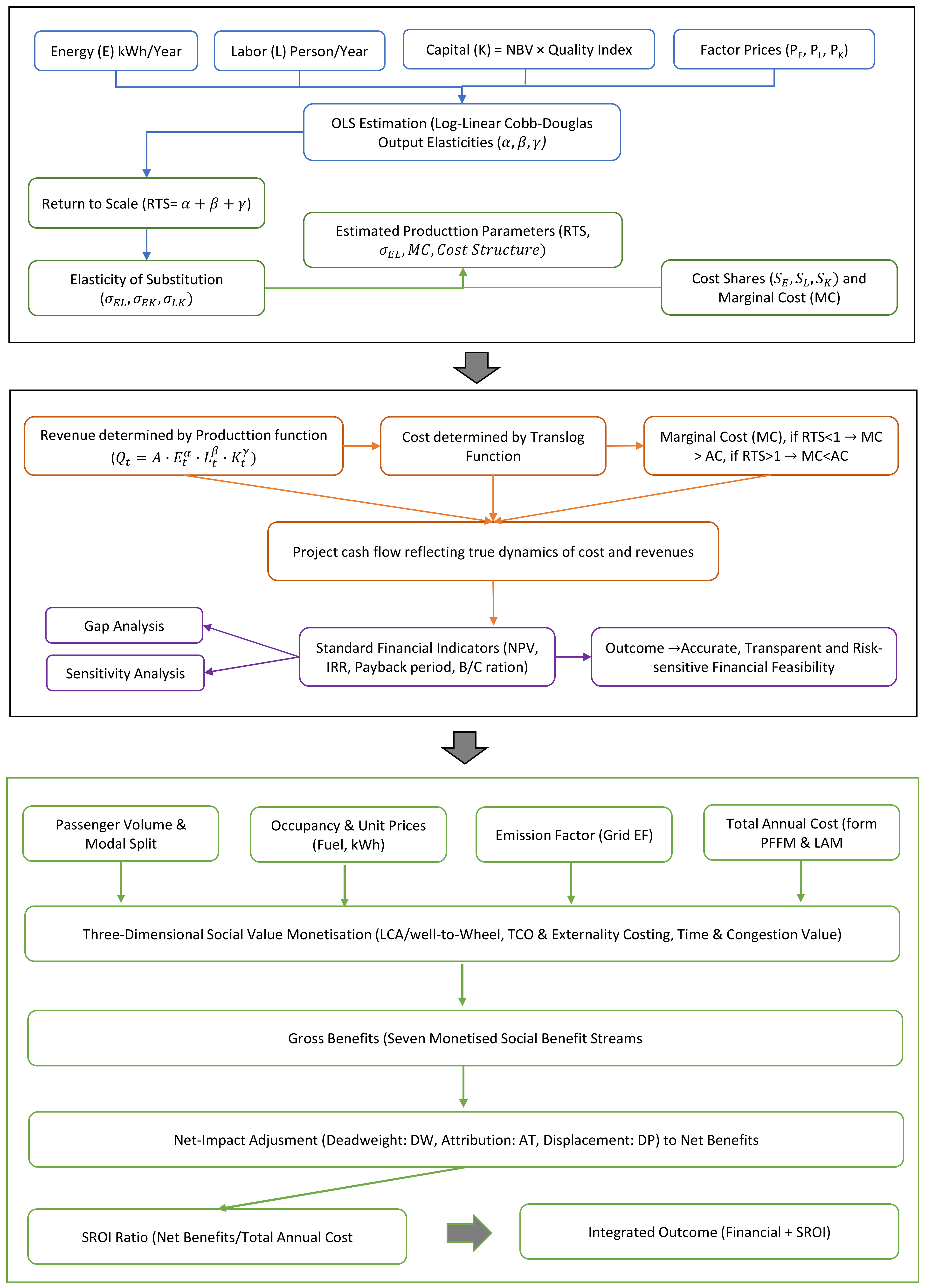
As shown in Figure 2, the study’s conceptual framework is based on a Production Function-Based Financial Feasibility Model (PFFM) comprising four interconnected layers. Layer 1 collects data on key production inputs, including electrical energy (E), labour (L), capital (K), and input prices. The output elasticities (α, β, and γ) are then estimated using OLS through the Cobb–Douglas production function. Layer 2 calculates returns to scale ($RTS=\alpha +\beta +\gamma$) and uses this value to compute marginal cost based on the relationship $MC=AC/RTS$, thereby reflecting a non-linear cost structure. Accordingly, this layer provides a set of production parameters, particularly RTS and MC that can be estimated from actual data. Layer 3 uses these parameters to formulate the financial assumptions. Revenue is determined by the production function, $Q_t=A{E}_t^{\alpha }{L}_t^{\beta }{K}_t^{\gamma }$, while marginal cost is derived from $MC=AC/RTS$, which differs significantly according to the estimated RTS value. In other words, when RTS < 1 and MC > AC, production costs increase faster than output. Conversely, when RTS > 1 and MC < AC, the project exhibits economies of scale. This layer therefore generates project cash flows that reflect the underlying dynamics of costs and revenues. Layer 4 uses cash flows to assess financial feasibility through standard indicators, including NPV, IRR, payback period, and B/C ratio. It also analyses project risk using three main tools: gap analysis comparing the PFFM with the LAM, sensitivity analysis, and worst-case scenario analysis. The framework further links the PFFM results to an SROI assessment that evaluates the broader social value generated by the public electric bus project. The SROI analysis monetises relevant social and environmental outcomes and compares their present value with the total investment required. This assessment distinguishes stand-alone financial feasibility from broader public value. Accordingly, the integrated framework provides decision-makers with both a transparent assessment of financial performance and a broader evaluation of the project’s social return and policy significance.

2.7.2. Key Assumptions Between the PFFM and LAM

Comparison of Assumption Structures

The comparison of assumption structures between the linear assumption model (LAM), which represents the traditional practice and the Production Function-Based Financial Feasibility Model (PFFM) developed in this study reveals clear systematic differences. These differences directly affect the accuracy of cash flow estimation and the ability to assess project risks (Shim & Kim, 2022).

Theoretical Foundations and Model Structure

The LAM is not supported by a foundation in production economics but relies on ad hoc assumptions that do not reflect the actual production mechanisms of public transportation enterprises. In contrast, the PFFM integrates the Cobb–Douglas production function, enabling the model structure to systematically capture the relationship between production inputs, including energy, labour, and capital, and output (passenger-kilometres), in accordance with duality theory (Christensen et al., 1973; Cobb & Douglas, 1928).

Mechanism for Formulating Revenue and Cost Assumptions

Under the LAM framework, revenues and costs are assumed to grow at a constant rate, such as 3% per year, without considering capacity constraints or input price volatility (Massot, 2014). In contrast, the PFFM uses parameters estimated from actual data to define revenue boundaries using the production function, as given by this equation: $Q_t=A\cdot E_t^{\alpha }\cdot L_t^{\beta }\cdot K_t^{\gamma }$. This allows future cash flows to change non-linearly according to output levels and input prices in an economically rational manner (Terblanche & Root, 2022).

Production Economics Parameters (RTS and MC)

The most obvious difference appears in the technical dimension of production. The LAM implicitly assumes that the project exhibits constant returns to scale (RTS = 1), and marginal cost is always equal to average cost (MC = AC), and the production inputs can be substituted without limit ($\sigma =\infty$). These assumptions contradict the actual conditions of public transportation systems, which are constrained by technology and labour capacity (Walters, 1963). In contrast, the PFFM does not predetermine these parameters, but estimates them from actual data through the Cobb–Douglas production function, yielding RTS values and the relationship (MC = AC/RTS) in accordance with the theory. In addition, Booth (1991) noted that production technologies with low elasticity of substitution ($\sigma <1$) expose enterprises to higher risks. The PFFM can employ such elasticity values from the literature to support risk analysis.

Capability to Detect Worst-Case Scenarios

The structural limitations of the LAM directly affect risk assessment. Under linear growth assumptions and fixed unit costs, the LAM’s net present value (NPV) tends to remain positive in normal scenarios. However, it fails to reflect the effects of severe changes in input prices (Blessing & Ifeanyi, 2025), leading to poor investment decisions and budget overruns. In contrast, the PFFM can effectively detect early warning signals by relying on RTS and marginal cost (MC) parameters estimated from actual data. These parameters reflect the project’s exposure to changes in input prices, resulting in its high vulnerability to energy-price volatility. This mechanism enables the PFFM to assess risks under worst-case scenarios significantly better than the LAM (Haass & Guzman, 2020).

Incorporation of Social Value Through SROI

Evaluated solely on standard financial indicators (NPV, IRR, Payback Period, B/C ratio), the Khon Kaen EV Bus project may appear commercially unviable, as public transport services of this nature inherently depend on government subsidies rather than full commercial self-financing (European Commission, 2014). This does not indicate a lack of merit but reflects the nature of public service provision, whose value extends beyond farebox revenue. The study therefore incorporates a social return on investment (SROI) analysis within the conceptual framework (Figure 2), capturing the extent to which the project raises residents’ standard of living through an integrated three-dimensional approach: Life-Cycle Assessment/Well-to-Wheel environmental impact (Martini et al., 2024), total cost of ownership and externality costing for health and accident impacts (Carbone et al., 2025), and net-impact adjustment for deadweight, attribution, and displacement (Nicholls et al., 2012), so that the overall assessment reflects both commercial and social returns.

3. Research Methodology

3.1. Research Methodology, Data Sources, and Research Framework

This study was conducted within a quantitative research framework, using secondary data from the feasibility study report system and the internal financial model of the Khon Kaen Provincial Administrative Organization (Chantuk et al., 2026). This report is the complete feasibility study report for the electric bus (EV bus) project in Mueang Khon Kaen District, aimed at providing public transportation services and reducing air pollution in Khon Kaen Province. The report was made under Contract No. 1/2025 by the Academic Service Bureau of Silpakorn University. The raw data were operationalised into a 15-year annual time-series dataset. It integrates actual operating assumptions with the passenger demand growth framework (3% per year based on the provincial transport development plan), a 10-year straight-line depreciation policy, and a battery replacement reserve fund in Year 8 (30% of the vehicle value for Route 2). The dataset was assessed for face validity by public transportation experts (Blessing & Ifeanyi, 2025).

The analytical framework of this study was designed as a sequential five-step analytical plan to ensure that the research process systematically and verifiably aligns with the four research objectives, as follows:

• Data acquisition, systematisation, and validation of secondary data from the Khon Kaen PAO feasibility report (Chantuk et al., 2026), including verification of internal consistency, completeness of all cost and revenue items, and reconciliation of route-level operating assumptions across the 15-year projection horizon.
• Estimation of the Cobb–Douglas production function using ordinary least squares (OLS) (Cobb & Douglas, 1928).
• Constructing systematic generation of revenue and expenditure assumptions for the PFFM and LAM models (financial assumption generation) (Massot, 2014; Terblanche & Root, 2022).
• Calculation of standard financial feasibility indicators (NPV, IRR, payback period, and B/C ratio) under the specified discount rate framework (WACC) (Shim & Kim, 2022).
• Conducting the test of gap analysis and sensitivity analysis with worst-case scenario to assess structural risk (Haass & Guzman, 2020).
• Conducting a social return on investment (SROI) analysis using an integrated three-dimensional evaluation approach that combines Life-Cycle Assessment/Well-to-Wheel environmental impact, total cost of ownership and externality costing, and net-impact adjustment to assess the social returns generated by the project beyond its financial performance (Martini et al.,2024; Carbone et al., 2025; Nicholls et al., 2012).

The detail of research methodology design corresponds to each research objective as follows: (1) the development of the conceptual framework and construction of the PFFM model to achieve the objective of developing a conceptual framework for public service projects. The researchers designed the workflow and mathematical equations to integrate production function parameters with the project cash flow structure in a unified manner, replacing linear growth assumptions with an economic mechanism that reflects actual production constraints (Walters, 1963). (2) Estimation of production economics parameters using the Cobb–Douglas production function, the researchers employed the ordinary least squares (OLS) econometric technique to estimate output elasticities and calculate returns to scale in accordance with production theory. (3) Gap analysis and risk detection.

To assess differences between the PFFM and the linear assumption model (LAM), this study compares key financial indicators, including NPV, IRR, PBP, and B/C ratio. It also conducts a sensitivity analysis using a worst-case scenario to empirically demonstrate that the traditional model overestimates project viability and fails to detect conditions in which NPV < 0 (Terblanche & Root, 2024) and to present the PFFM as a prototype methodology. To enable the broader application of the PFFM to public investment projects, the model was assessed for face validity by public transportation experts in order to confirm the stability of the results under uncertainty in key parameters before proposing a framework for applying the model to other types of public services in developing countries (Stadtherr & Wouters, 2021).

3.2. Research Data

The data used in this study consist of secondary data obtained from the complete feasibility study report for the electric bus (EV bus) project in Mueang Khon Kaen District, Khon Kaen Province, prepared by Chantuk et al. (2026) under Contract No. 1/2025 by the Academic Service Office of Silpakorn University. The data presented in

Table 1. CAPEX data for the EV bus project of Khon Kaen Provincial Administrative Organization (Year 0).

No	List	Number	Unit	Price/Unit (Baht)	Total (Baht)
A	Rolling stock (EV buses and on-board equipment)				251,999,990
A1	Mini EV bus, 7.6 m (Route 1): 15 operating units + 1 reserve unit	16	Vehicle	4,500,000	72,000,000
A2	Large EV bus, 12 m (Route 2): 10 operating units + 1 reserve unit	11	Vehicle	7,500,000	82,500,000
A3	Medium EV bus, 8.5 m (Route 3): 15 operating units + 1 reserve unit	16	Vehicle	5,500,000	88,000,000
A4	On-board equipment and spare parts (43 vehicles in total)	43	Vehicle	220,930	9,499,990
B	Infrastructure and charging stations (all 3 routes)				19,970,000
B1	OCC, transformer, charging station, and bus terminal (Route 2)	1	Set	7,870,000	7,870,000
B2	Transformer, charging station, bus terminal, and site preparation (Route 3)	1	Set	7,280,000	7,280,000
B3	Transformer, charging station, and bus terminal (Route 1)	1	Set	4,820,000	4,820,000
C	Smart and standard bus stops (all 3 routes)				8,160,000
C1	Bus stop type B (smart): 10 + 10 + 10 stops × 150,000 Baht	30	Stop	150,000	4,500,000
C2	Bus stop type C (standard): 27 + 19 + 15 stops × 60,000 Baht	61	Stop	60,000	3,660,000
D	IT system, welfare cards, licenses, and buildings (all 3 routes)				4,921,300
D1	Bus operation application system (primarily for Route 2)	1	System	500,000	500,000
D2	Welfare cards (initial stock for all three routes)	40,000	Card	50	2,000,000
D3	Knock-down office buildings (Routes 1 and 3)	2	Site	500,000	1,000,000
D4	Bus operating licence fees (3 routes × 7100 Baht)	3	Route	7100	21,300
D5	Pre-operating expenses, working capital, and land rental fee (Year 0)		as planned		1,400,000
Total CAPEX (A + B + C + D)					285,051,290

,

Table 2. Route-level production input data (Year 1).

Parameter	Route 1 Mini Bus—7.6 m	Route 2 Large Bus—12 m	Route 3 Medium Bus—8.5 m	Total/Average
Total number of vehicles (operating + reserve)	16 (15 + 1)	11 (10 + 1)	16 (15 + 1)	43
Number of actual operating vehicles	15	10	15	40
Total service distance, Et-km (km/year)	831,965	735,316	581,915	2,149,196
Total electricity consumption, Et (kWh/year)	665,572	882,379	581,915	2,129,866
Energy consumption rate (kWh/km)	0.80	1.20	1.00	0.99 average
Electricity price, pE (Baht/kWh)	3.20	3.20	3.20	3.20
Total personnel, Lt (persons)	18	14	20	52
Average wage, pL (thousand Baht/person/month)	18.9	19.1	18.9	19.0
Cost of capital, pK (depreciation/vehicle/year, million Baht)	0.300	0.750	0.367	0.460
Fare revenue (million Baht/year)	5.97	10.32	8.10	24.39
Advertising revenue (million Baht/year)	2.04	1.44	2.04	5.52
Total revenue, Rt (million Baht/year)	8.01	11.76	10.14	29.91
Total OPEX (million Baht/year)	8.93	9.21	9.18	27.32

and

Table 3. Fifteen-year annual dataset for production function estimation.

Year	${\mathit{Q}}_{\mathit{t}}$	${\mathit{E}}_{\mathit{t}}$	${\mathit{L}}_{\mathit{t}}$	${\mathit{K}}_{\mathit{t}}$	${\mathit{p}}_{\mathit{E}}$	${\mathit{p}}_{\mathit{L}}$	TC * = OPEX	AC	${\mathit{D}}_{\mathit{t}}$	Remark
1	8.50	2.13	52.00	1.00	3.20	19.00	27.32	3.21	27.77	Base year
2	8.76	2.19	53.00	0.90	3.30	19.60	28.00	3.20	27.77	Qt + 3%/year
3	9.02	2.26	54.00	0.80	3.40	20.20	28.70	3.18	27.77	pE + 3.1%/year
4	9.29	2.33	55.00	0.70	3.51	20.80	29.42	3.17	27.77	pL + 3.0%/year
5	9.57	2.40	56.00	0.60	3.62	21.40	30.16	3.15	27.77
6	9.85	2.47	57.00	0.50	3.73	22.00	30.91	3.14	27.07
7	10.15	2.54	58.00	0.40	3.84	22.70	31.68	3.12	27.07
8	10.45	2.62	59.00	0.30	3.96	23.40	57.22	5.48	27.07	Battery replacement: THB 24.75 million
9	10.77	2.70	60.00	0.20	4.09	24.10	33.29	3.09	27.07	Kt remains constant after Year 8
10	11.09	2.78	61.00	0.10	4.21	24.80	34.12	3.08	27.07
11	11.42	2.86	62.00	0.42	4.34	25.50	34.97	3.06	1.87	Kt recovery/Dt decreases
12	11.77	2.95	63.00	0.42	4.48	26.30	35.85	3.05	1.87
13	12.12	3.04	64.00	0.42	4.62	27.10	36.74	3.03	1.87
14	12.48	3.13	65.00	0.42	4.76	27.90	37.66	3.02	1.87
15	12.86	3.22	66.00	0.42	4.91	28.70	38.60	3.00	1.87
Average	10.54	2.64	59.00	0.51	4.00	23.57	34.31	3.26	18.90

Note: * TC (total cost) = OPEX (Khon Kaen Provincial Administrative Organization is a government agency; corporate income tax is not applicable).

consist of three main datasets: (1) investment costs (CAPEX) in Year 0, classified by expenditure category, including rolling stock, infrastructure and charging stations, bus stops, IT systems, welfare card, buildings, licences, and pre-operating and working capital; (2) route production inputs in Year 1 for each route, namely Route 1 Mini, Route 2 Large, and Route 3 Medium, including distance, electricity power, electricity consumption rate, electricity price, personnel, wages, costs, revenues, and OPEX; and (3) a 15-year annual dataset for estimating the production function, covering the variables such as Q_t, E_t, L_t, K_t, p_E, p_L, and total cost (TC), together with assumptions regarding growth rates and the battery replacement fund in Year 8. The three-route structure characterised by differences in vehicle size, service distance, and energy consumption rates is consistent with practices identified in the literature. Previous studies indicate that EV bus systems comprising multiple route types require route-specific total cost of ownership (TCO) analysis over the project life-cycle, as the TCO of electric buses varies significantly according to route characteristics and operating schedules (Dydkowski et al., 2021; Grauers et al., 2020; Lotfi et al., 2020).

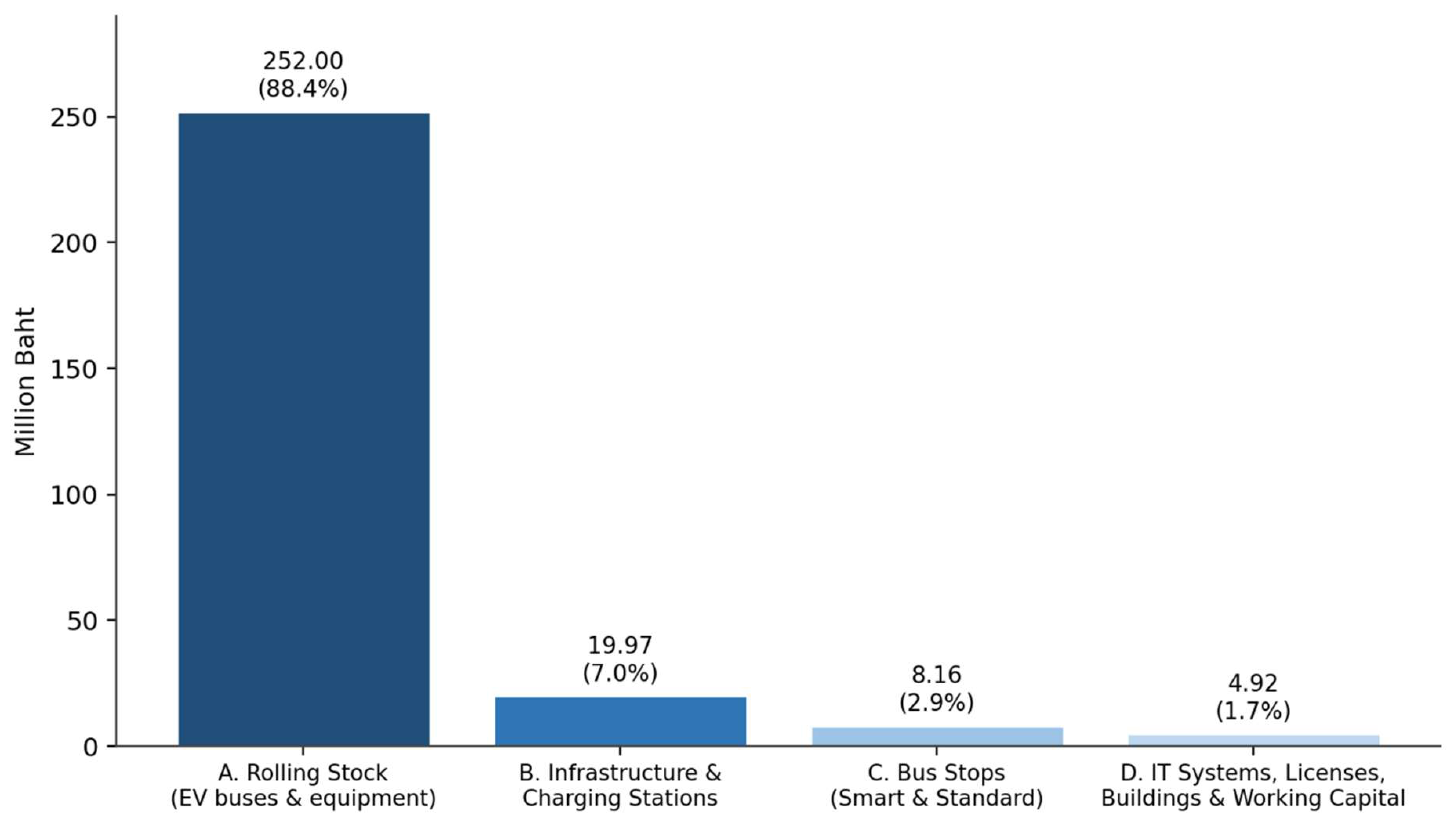
As presented in Figure 3, the total capital expenditure (CAPEX) of the project amounts to THB 285.05 million. The largest proportion is allocated to rolling stock, comprising electric buses and related equipment, with an investment value of THB 252.00 million, representing 88.4% of total CAPEX. Infrastructure and charging stations constitute THB 19.97 million, or 7.0%, while the development of bus stops accounts for THB 8.16 million, equivalent to 2.9%. The remaining THB 4.92 million, or 1.7%, is allocated to information technology systems, licenses, buildings, and working capital. These findings indicate that the project’s capital structure is highly concentrated in the acquisition of electric buses and associated equipment, which represents the principal component of the initial investment.

Explanation of Symbols in Table 3.

$Q_t$ = Output volume (total service distance) (million kilometres).

$E_t$ = Electricity consumption (million kWh).

$L_t$ = Number of personnel (persons).

$K_t$ = Capital utilisation index derived from net asset value divided by initial asset value under straight-line depreciation. The index is reset in Year 11 due to the battery investment in Year 8 (investing in the battery investment in Year 8 makes K_t recover).

$p_E$ = Electricity price (Baht/kWh).

$p_L$ = Average wage (thousand Baht/person/month).

$OPE{X}_t$ = Total operating expenditure (million Baht).

$T{C}_t$ = Total cost (million Baht). In this study, $T{C}_t=OPE{X}_t$.

$A{C}_t$ = Average cost per unit, calculated as $T{C}_t/Q_t$ (Baht/km).

$D_t$ = Annual depreciation (million Baht).

With the exception of Year 1, which relies on route-level operating assumptions outlined in the underlying feasibility report (Chantuk et al., 2026), the projections for Years 2–15 in Table 3 are deterministic estimates based on the assumed annual growth rates indicated in the Remarks column (Q_t + 3%/yr, p_E + 3.1%/yr, p_L + 3.0%/yr, an additional staff member annually, and the straight-line depreciation schedule associated with K_t). These growth rates have been validated by experts from EV bus operating companies in Thailand. As this is a feasibility study for a project that has not yet commenced operations, the 15-year series is based on projections rather than on actual operational data. Therefore, Equation (2) is primarily used to evaluate the internal consistency of the assumed cost-output structure within the Cobb–Douglas framework, confirming the coherence of the technical assumptions.

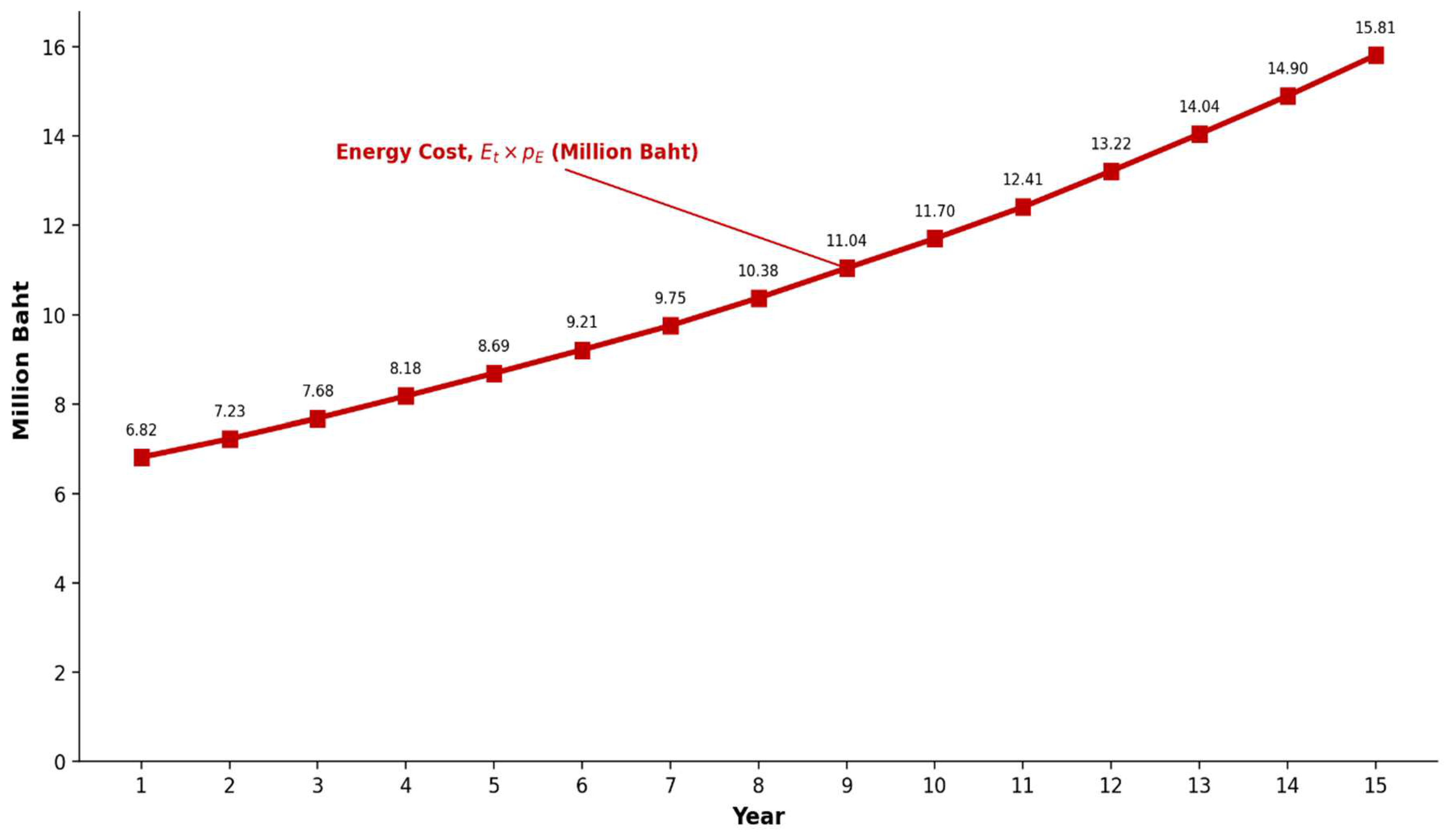
The projected trends in energy-cost ($E_t$ × $p_E$) over the 15-year project life-cycle are illustrated in Figure 4.

As shown in Figure 4, the annual energy cost $\left(E_t×p_E\right)$ increases continuously throughout the 15-year project period, rising from THB 6.82 million in Year 1 to THB 15.81 million in Year 15. The convex upward trend indicates that energy expenditure increases at an accelerating rate over time. Under the assumptions of the financial model, this pattern results from the combined effects of increasing electricity consumption and the annual escalation of electricity prices. Consequently, energy cost becomes an increasingly important component of the project’s operating expenditure and may exert greater pressure on its long-term financial feasibility.

3.3. Functional Form Specification and Parameter Estimation

3.3.1. Cobb–Douglas Production Function

This study specifies a Cobb–Douglas production function with three production inputs, namely electricity energy (E_t), labour (L_t), and capital (K_t), as follows:

$$Q_t=A\cdot E_t^{\alpha }\cdot L_t^{\beta }\cdot K_t^{\gamma }\cdot e^{{\epsilon }_t}$$

(1)

For ease of estimation using ordinary least squares (OLS), Equation (1) is transformed into a log-linear form.

$$\ln Q_t=a_0+\alpha \ln E_t+\beta \ln L_t+\gamma \ln K_t+{\epsilon }_t$$

(2)

where $a_0=\mathrm{l}\mathrm{n}A$ and ${\epsilon }_t$ denotes the random error term.

Returns to scale (RTS) are calculated as the sum of the estimated output elasticities:

$$RTS=\alpha +\beta +\gamma$$

If $RTS=1$, this indicates constant returns to scale (CRS).

If $RTS>1$, this indicates increasing returns to scale (IRS).

If $RTS<1$, this indicates decreasing returns to scale (DRS).

Marginal cost (MC) can be calculated using the relationship between average cost ($AC=C/Q$) and returns to scale ($RTS$).

$$MC={\displaystyle \frac{C}{Q}}\times {\displaystyle \frac{1}{RTS}}$$

(3)

where $C$ denotes total cost, and $Q$ denotes output in year $t$. Equation (3) shows that if $RTS<1$, then $MC>AC$, meaning that marginal cost is higher than average cost.

3.3.2. Cash Flow Equation

The EV bus project is operated by the Khon Kaen Provincial Administrative Organization. This government agency is not subject to corporate income tax. It relies on annual budget appropriations, including local taxes and government subsidies, as its funding sources, with no financial debt obligations. The net cash flow in each year is calculated as follows:

$$C{F}_t={\mathrm{Revenue}}_t-{\mathrm{Cost}}_t$$

(4)

where

$C{F}_t$ = Net cash flow of the project in year $t$ (Baht);

${\mathrm{Revenue}}_t$ = Total operating revenue in year $t$ (Baht);

${\mathrm{Cost}}_t$ = Total operating cost (excluding depreciation) in year $t$ (Baht).

3.3.3. Discount Rate

Since the project is financed through public budget allocations without debt financing, this study specifies a social discount rate of 7.5%, reflecting the opportunity cost of public funds. This rate is derived from the 10-year government bond yield of approximately 4.5% plus a project-specific risk premium of 3.0%. It also falls within the standard range of 7–10% for public infrastructure projects with moderate to high risk in developing countries (Shim & Kim, 2022).

3.3.4. Financial Indicators and Gap Analysis

This study evaluates financial feasibility using key indicators, including net present value (NPV), internal rate of return (IRR), payback period (PBP), and benefit-cost ratio (B/C). The discount rate is set at $r=7.5\%$. The NPV formula is presented in Equation (5).

$$NPV=-CAPEX+{\sum }_{t=1}^{15}{\displaystyle \frac{{CF}_t}{{\left(1+r\right)}^t}},r=7.5\%$$

(5)

where $CAPEX$ denotes the initial investment of 285.05 million Baht as presented in Table 1, and $C{F}_t$ represents the net cash flow in year $t$ calculated using Equation (4). IRR is the discount rate ($r$) that makes $NPV=0$, which is calculated through interval estimation. To compare the differences between the PFFM and the traditional linear assumption model (LAM), this study analyses the net present value gap, as expressed in Equation (6).

$$Ga{p}_{NPV}\left(\%\right)={\displaystyle \frac{NP{V}^{LAM}-NP{V}^{PFFM}}{\mid NP{V}^{PFFM}\mid }}\times 100\%$$

(6)

$Ga{p}_{NPV}>0$ indicates that the LAM overestimates the project value compared to the PFFM. The absolute value of $NP{V}^{PFFM}$ is used in the denominator to ensure that the formula remains applicable even when $NP{V}^{PFFM}$ is negative, such as under a worst-case scenario.

3.4. Social Return on Investment (SROI): Analytical Approach, Formulation, and Baseline Data

Because public transport projects such as the EV bus service generate substantial value through unpriced externalities—reduced air pollution, improved road safety, and time savings—that farebox revenue alone does not capture (European Commission, 2014), this study supplements the financial feasibility analysis in Section 4 with a social return on investment (SROI) analysis, using an integrated three-dimensional evaluation framework that combines Life-Cycle Assessment/Well-to-Wheel analysis of environmental impact (Martini et al., 2024), total cost of ownership and externality costing for health and accident impacts (Carbone et al., 2025), and a net-impact adjustment for deadweight, attribution, and displacement (Nicholls et al., 2012).

3.4.1. Baseline Scenario, Data, and SROI Formulation

Following the Khon Kaen PAO feasibility assessment (Chantuk et al., 2026), the baseline (counterfactual) scenario assumes that, in the absence of the EV bus project, the 11,497 weekday passengers across the three routes would travel by motorcycle (40%; occupancy of 1.1 persons/vehicle), private car (30%; occupancy of 1.5 persons/vehicle), or diesel songthaew (30%; occupancy of 10 persons/vehicle), consistent with the Modal Split assumptions in Table 2. Fuel and electricity prices are as of February 2026 (diesel = 29.49 Baht/liter; gasohol 95 = 30.85 Baht/liter; electricity = 3.75 Baht/kWh, inclusive of the Ft adjustment), and the Grid Emission Factor for Thailand is 0.4999 kgCO₂e/kWh (Thailand Greenhouse Gas Management Organization, 2023). The SROI ratio is calculated as the ratio of adjusted net social benefits to the project’s total annual cost, as shown in Equation (7).

SROI = Net Benefits ÷ Total Annual Cost

(7)

where net benefits are obtained by discounting the Gross Benefits (Section 3.4.2) using three net-impact adjustment factors, as shown in Equation (8)

Net Benefits = Gross Benefits × (1 − DW) × (1 − AT) × (1 − DP)

(8)

Deadweight (DW) represents the share of the outcome that would have occurred without the project; attribution (AT) represents the share attributable to other agencies’ initiatives; and displacement (DP) represents any negative outcome the project causes elsewhere (e.g., displaced local operators). Consistent with the project’s public-sector-led rollout and its explicit integration of incumbent songthaew operators into the service model, this study sets DW = 5%, AT = 5%, and DP = 0% (

Table 4. Net-impact adjustment factors applied to gross social benefits.

Factor	Value	Retained Share	Rationale
Deadweight (DW)	5%	0.95	The likelihood of a comparable EV bus system emerging without PAO-led investment is low.
Attribution (AT)	5%	0.95	Measured ridership and modal shift can be primarily attributed to the Khon Kaen PAO service.
Displacement (DP)	0%	1.00	The Songthaew operators have been integrated into the service rather than being displaced.
Drop-off (DO)	0%	1.00	The benefits are expected to either persist or increase with ridership, and therefore this factor is not applied in Equation (8).

Source: Compiled by the researchers based on the study of Chantuk et al. (2026).

). A drop-off (DO) rate of 0% is assumed because benefits are expected to persist or grow with ridership over the appraisal horizon and is therefore not applied as a separate multiplicative discount in Equation (8).

3.4.2. Monetised Social Benefit Stream Methodology

By considering the vehicle-kilometres travelled (VKT) avoided through the modal shift to electric bus (EV bus), along with the associated emission factors, damage costs, and unit price parameters outlined above, seven distinct benefit streams are monetised annually. These include (i) net energy-cost savings, derived from the difference between avoided fuel expenditure and the project’s electricity expenses; (ii) net maintenance cost savings, reflecting the reduced upkeep costs of EV buses compared to conventional vehicles; (iii) the valuation of avoided health damage costs resulting from decreased exposure to PM_2.5, NO_x, and CO₂, using damage costs consistent with the methodologies of Carbone et al. (2025); (iv) the monetary value assigned to reduced greenhouse gas emissions based on a carbon price of 500 Baht per ton of CO₂ equivalent; (v) avoided accident costs, stemming from decreased motorcycle and private car kilometres travelled; (vi) the economic benefits of reduced traffic congestion and travel-time losses for other road users; and (vii) local economic uplift attributable to improved travel convenience. The aggregate Gross Benefits, along with net benefits and the social return on investment (SROI) ratio, are further detailed and analysed in Section 4.4.

4. Results

4.1. Estimation of the Cobb–Douglas Production Function

According to the 15-year annual dataset presented in Table 3 and the model specified in Equation (2), this study estimates the Cobb–Douglas production function using ordinary least squares (OLS) based on the log-linear relationship as follows:

$$\mathrm{l}\mathrm{n}{Q}_t=a_0+\alpha \mathrm{l}\mathrm{n}{E}_t+\beta \mathrm{l}\mathrm{n}{L}_t+\gamma \mathrm{l}\mathrm{n}{K}_t+{\epsilon }_t$$

The dependent variable is $\ln Q_t$ (output volume (million kilometres)). The independent variables consist of $\ln E_t$ (electricity consumption/million kWh), $\ln L_t$ (labour/person), and $\ln K_t$ (the capital utilisation index), which reflects the level of asset utilisation and capital efficiency in each year. The estimation was conducted using OLS with HAC (Newey–West) standard errors, employing the Bartlett kernel and a bandwidth of 1 to ensure that the standard errors are robust to serial correlation and heteroskedasticity. The estimation results are summarised in

Table 5. Estimation results of the Cobb–Douglas production function developed from Gretl.

Variable	Coefficient	Std. Error (HAC)	t-Ratio	p-Value
Constant ($a_0$)	1.32999	0.329060	4.04	0.0019 ***
$\ln E_t$ ($\alpha$)	0.99025	0.053697	18.44	0.001 ***
$\ln L_t$ ($\beta$)	0.01561	0.093489	0.16	0.8704
$\ln K_t$ ($\gamma$)	0.00034	0.000299	1.14	0.2752

Note: *** denotes statistical significance at the 0.1% level (p < 0.001).

.

$$\begin{array}{cccc}{R}^2& =0.999953\hfill & \mathrm{Adjusted}{R}^2& =0.999940\hfill \\ \mathrm{S}.\mathrm{E}.\mathrm{of}\mathrm{regression}& =0.001023\hfill & \mathrm{Durbin-Watson}& =2.008\hfill \\ \mathrm{Log-likelihood}\left(\ln \mathrm{Q}\right)& =84.319\hfill & \mathrm{Log-likelihood}\left(\mathrm{Q}\right)& =49.114\hfill \end{array}$$

4.1.1. Elasticities of Output and Returns to Scale (RTS)

The coefficients for all production inputs have signs consistent with economic theory. Electricity has a high output elasticity ($\alpha =0.99025$) and is statistically significant at the 0.001 level. Labour and capital have low elasticities ($\beta =0.01561$, $\gamma =-0.00034$). They are not statistically significant, as changes in labour and the capital utilisation index during the study period were relatively small compared with changes in electricity consumption. Overall, the model explains output variation very well, with $Adjusted{R}^2=0.999940$. The Durbin–Watson statistic is 2.008, indicating no significant autocorrelation problem in the error terms.

Although the coefficients of labour ($L_t$) and capital ($K_t$) are not statistically significant due to their strong structural relationship with electricity consumption ($E_t$) in the production process, the researchers retained all three variables in the model to reflect the complete cost structure of the public transportation enterprise. This decision is consistent with the observation by Felipe and Adams (2005), who noted that in real production contexts, production inputs are often inseparable and interdependent. Removing variables from the model solely because they lack statistical significance may introduce specification bias, particularly when such factors are technologically fixed inputs that must operate together with energy to generate output. Therefore, retaining the variables $L$ and $K$ enables the PFFM to estimate returns to scale (RTS) and marginal cost (MC) more comprehensively, while reflecting the actual characteristics of production technology more accurately than considering only statistically significant factors. Returns to scale (RTS) are calculated as the sum of the output elasticities in accordance with production theory, as follows:

$$RTS=\alpha +\beta +\gamma =0.99025+0.015608+0.000344=1.00620$$

RTS > 1 indicates increasing returns to scale (IRS). In other words, a 1% increase in all production inputs would result in an approximately 1.00620% increase in output, which is greater than the proportional increase in inputs. This finding is consistent with the characteristics of public transportation enterprises, which typically have high fixed-cost structures and can achieve economies of scale as passenger volume increases. However, the estimated RTS value is 1.00620, which is very close to 1. This indicates approximately constant returns to scale, a common characteristic of public transportation enterprises operated by government agencies such as the Khon Kaen Provincial Administrative Organization. This is similar to the result of the retrospective analysis of Felipe and Adams (2005), which indicated that, in many cases of production function estimation, the resulting estimates tend to yield an aggregate elasticity close to 1. Such results reflect a high degree of structural interdependence among production inputs, resembling the accounting identity underlying income distribution. As the PFFM produces results of this nature, it therefore confirms the validity of the data and the estimation process, indicating that the model can comprehensively capture the relationships among key production inputs, namely energy, labour, and capital, in accordance with the theoretical framework, even in a context where these inputs are highly interdependent.

A methodological issue arises regarding whether Equation (2) genuinely captures an independent production technology. Since electricity consumption in the dataset is derived from service distance multiplied by a fixed energy consumption rate per kilometre (kWh/km), as verified by experts from EV bus operating companies in Thailand, this ratio remains nearly constant over the 15-year period (ranging from 3.987 to 4.000, a variation of only 0.33%; see Table 3). Consequently, they differ by an approximately fixed constant. Under these conditions, an ordinary least squares (OLS) regression of output on input tends to yield an estimated elasticity close to 1 and an almost perfect coefficient of determination, regardless of the true underlying production relationship. In line with Felipe and Adams (2005), Cobb–Douglas regressions on such series may reflect the technical identity utilised in the data construction rather than an independently varying technology. Therefore, the coefficient should be interpreted as confirming the internal consistency of the assumed energy consumption rate across the projection period, rather than serving as an independent empirical estimate.

4.1.2. Calculation of Marginal Cost

Based on Equation (3), marginal cost ($MC$) can be calculated from average cost ($AC=C/Q$) and returns to scale ($RTS$) as follows:

$$MC={\displaystyle \frac{C}{Q}}\times {\displaystyle \frac{1}{RTS}}=AC\times {\displaystyle \frac{1}{RTS}}$$

Using the average cost over the 15-year dataset ($A{C}_{\mathrm{Average}}$ = 3.26 Baht/km) and the calculated returns to scale ($RTS=1.00620$), the marginal cost is calculated as follows:

$$MC=3.26\times {\displaystyle \frac{1}{1.00620}}=3.24\mathrm{Baht}\mathrm{per}\mathrm{kilometre}$$

(9)

The estimated marginal cost of 3.24 Baht/km is lower than the average cost of 3.26 Baht/km, indicating economies of scale. This means that producing one additional unit of output would increase cost by less than the existing average cost. Therefore, the EV bus project of the Khon Kaen Provincial Administrative Organization still has the potential to reduce unit costs if passenger service distance can be expanded. This finding is useful for planning future route expansion and increasing service frequency.

The estimated RTS of 1.00620 exceeds unity. Testing the null hypothesis using the HAC standard errors reported in Table 4 shows that RTS is not statistically distinguishable from constant returns to scale at any conventional significance level. Since MC is derived from the equation $MC=AC/RTS$ (Equation (3)), an RTS of 1.00620 implies that economies of scale are not clear; the estimate merely indicates a tendency or potential for increasing returns to scale in the EV bus project. Furthermore, the NPV gap between PFFM and LAM ($Ga{p}_{NPV}=-0.05\%$) is very small. Nevertheless, in this study, the finding suggests that the PFFM may provide a more appropriate estimate than the LAM.

4.2. Gap Analysis Between the PFFM and LAM Models

4.2.1. Cost Assumption Specification Based on the Estimated Production Structure

Based on the production function estimation in Section 4.1, the estimated RTS is 1.0062. Although this value is close to 1, it remains greater than 1 and therefore still reflects economies of scale. This is consistent with the characteristics of public service projects, which involve certain fixed costs and exhibit improved production efficiency as the scale of operations expands.

These parameters were used to establish the cost assumptions for the PFFM by estimating marginal cost (MC) and fixed cost (FC) from the first year of operation (OPEX₁ = 27.32 million Baht; Q₁ = 8.50 million kilometres). Year 1 was selected as the base year to define the model’s cost structure throughout the project life-cycle.

Specifically, marginal cost was estimated using the average operating cost in the base year together with the estimated returns to scale, as follows:

$$MC={\displaystyle \frac{A{C}_1}{RTS}}={\displaystyle \frac{27.32/8.50}{1.0062}}={\displaystyle \frac{3.2141}{1.0062}}=3.1945\mathrm{Baht}/\mathrm{km}$$

The value of MC = 3.1945 Baht/km is the key parameter used in the PFFM throughout the analysis. To verify consistency with the full dataset, marginal cost can also be calculated from the 15-year average cost (AC_Average = 3.26 Baht/km), yielding MC_Average = 3.26/1.0062 = 3.24 Baht/km, which is close and confirms the model’s internal consistency. However, the PFFM applies MC = 3.1945 Baht/km from Year 1 to calculate the fixed cost (FC), which exactly balances the Year 1 operating expenditure (OPEX₁ = FC + (MC × Q₁)).

The fixed cost is then obtained by subtracting total variable cost from Year 1 operating expenditure:

$$\begin{array}{cc}FC& =OPE{X}_1-\left(MC\cdot Q_1\right)\hfill \\ & =27.32-\left(3.1945\times 8.50\right)\hfill \\ & =27.32-27.1533\hfill \\ FC& =0.1667\mathrm{million}\mathrm{Baht}/\mathrm{year}\hfill \end{array}$$

For the LAM, which represents the conventional approach, a constant variable cost per unit is calculated from the first-year data, assuming that there is no fixed cost ($FC=0$), as follows:

$$AV{C}_{LAM}={\displaystyle \frac{OPE{X}_1}{Q_1}}=3.2141\mathrm{Baht}\mathrm{per}\mathrm{Kilometre}$$

The operating cost, excluding depreciation, in year $t$ for each model is specified as follows:

LAM	PFFM
$Cos{t}_t^{LAM}=AV{C}_{LAM}\cdot {(Q}_t+B_t)$	$Cos{t}_t^{PFFM}=FC+MC\cdot {(Q}_t+B_t)$

The structural difference between the two models becomes obvious from Year 3 onward, when Q_t > Q₁ because the PFFM incorporates a constant fixed cost of 0.1667 million Baht per year and a marginal cost of 3.1945, which is lower than AVC_LAM of 3.2141. As a result, Cost_t^PFFM < Cost_t^LAM in every year, except in Year 1, when both models generate the same cost value. This is consistent with the principle that when RTS > 1 and MC < AC, the PFFM can reflect the cost structure, whereas the LAM cannot.

The cash flows and financial indicators of the PFFM and LAM can then be compared using the cost equations derived in Section 4.2.1, based on the data presented in Table 1, Table 2 and Table 3 and an annual discount rate of 7.5%. The present value (PV) analysis is presented in

Table 6. Comparative calculation of the PFFM and LAM models (Years 1–15).

Year	${\mathit{Q}}_{\mathit{t}}$ (Million km.)	${\mathit{R}}_{\mathit{t}}$ (Million THB)	$\mathit{C}\mathit{o}\mathit{s}{\mathit{t}}_{\mathit{t}}^{\mathit{L}\mathit{A}\mathit{M}}$ (Million THB)	$\mathit{C}\mathit{o}\mathit{s}{\mathit{t}}_{\mathit{t}}^{\mathit{P}\mathit{F}\mathit{F}\mathit{M}}$ (Million THB)	${\mathit{D}}_{\mathit{t}}$ (Million THB)	$\mathit{C}{\mathit{F}}_{\mathit{t}}^{\mathit{L}\mathit{A}\mathit{M}}$ (Million THB)	$\mathit{C}{\mathit{F}}_{\mathit{t}}^{\mathit{P}\mathit{F}\mathit{F}\mathit{M}}$ (Million THB)	$\mathit{P}{\mathit{V}}_{\mathit{t}}^{\mathit{L}\mathit{A}\mathit{M}}$	$\mathit{P}{\mathit{V}}_{\mathit{t}}^{\mathit{P}\mathit{F}\mathit{F}\mathit{M}}$
1	8.50	29.91	27.32	27.32	27.77	2.59	2.59	2.41	2.41
2	8.76	30.81	28.16	28.16	27.77	2.65	2.65	2.29	2.29
3	9.02	31.73	29.00	28.99	27.77	2.73	2.74	2.20	2.21
4	9.29	32.68	29.87	29.86	27.77	2.81	2.82	2.10	2.11
5	9.57	33.66	30.76	30.75	27.77	2.90	2.91	2.02	2.03
6	9.85	34.67	31.66	31.65	27.07	3.01	3.02	1.95	1.96
7	10.15	35.71	32.63	32.61	27.07	3.08	3.10	1.86	1.87
8	10.45	36.79	58.34	58.32	27.07	−21.55	−21.53	−12.08	−12.07
9	10.77	37.89	34.62	34.60	27.07	3.27	3.29	1.71	1.72
10	11.09	39.03	35.64	35.62	27.07	3.39	3.41	1.65	1.66
11	11.42	40.20	36.71	36.68	1.87	3.49	3.52	1.58	1.59
12	11.77	41.40	37.83	37.80	1.87	3.57	3.60	1.50	1.51
13	12.12	42.64	38.96	38.93	1.87	3.68	3.71	1.44	1.45
14	12.48	43.92	40.12	40.09	1.87	3.80	3.83	1.38	1.39
15	12.86	45.24	41.34	41.30	1.87	3.90	3.94	1.32	1.33
Total PV								13.33	13.46

Note: $\mathrm{C}\mathrm{o}\mathrm{s}{\mathrm{t}}_{\mathrm{t}}^{\mathrm{L}\mathrm{A}\mathrm{M}}=3.2141\times {(\mathrm{Q}}_{\mathrm{t}}+{\mathrm{B}}_{\mathrm{t}})$, $\mathrm{C}\mathrm{o}\mathrm{s}{\mathrm{t}}_{\mathrm{t}}^{\mathrm{P}\mathrm{F}\mathrm{F}\mathrm{M}}=0.1667+3.1945\times ({\mathrm{Q}}_{\mathrm{t}}+{\mathrm{B}}_{\mathrm{t}})$, $\mathrm{C}{\mathrm{F}}_{\mathrm{t}}={\mathrm{R}}_{\mathrm{t}}-\mathrm{C}\mathrm{o}\mathrm{s}{\mathrm{t}}_{\mathrm{t}}$,$\mathrm{P}{\mathrm{V}}_{\mathrm{t}}=\mathrm{C}{\mathrm{F}}_{\mathrm{t}}/(1.075{)}^{\mathrm{t}}$.

.

4.2.2. Base-Case Cash Flows and Financial Indicators

The net cash flow in year $t$ is calculated using Equation (4), based on revenue ($R_t$), which grows at 3% per year from $R_1$ of 29.91 million Baht, as presented in Table 2, and the initial investment, $CAPEX$ of 285.05 million Baht, as presented in Table 1. The cash flows are discounted using a discount rate of $r=7.5\%$.

The calculation of financial indicators based on Table 5 can be presented as follows:

(1)

The net present value (NPV), based on the initial investment of CAPEX = 285.05 million Baht as presented in Table 1, is calculated as follows:

$\mathit{N}\mathit{P}{\mathit{V}}^{\mathit{L}\mathit{A}\mathit{M}}$	$\mathit{N}\mathit{P}{\mathit{V}}^{\mathit{P}\mathit{F}\mathit{F}\mathit{M}}$
$-271.74\mathrm{m}\mathrm{i}\mathrm{l}\mathrm{l}\mathrm{i}\mathrm{o}\mathrm{n}\mathrm{B}\mathrm{a}\mathrm{h}\mathrm{t}$	$-271.61\mathrm{m}\mathrm{i}\mathrm{l}\mathrm{l}\mathrm{i}\mathrm{o}\mathrm{n}\mathrm{B}\mathrm{a}\mathrm{h}\mathrm{t}$

(2)

The internal rate of return (IRR) is calculated by estimating the discount rate ($r$) that makes $NPV=0$, based on the series of cash flows $C{F}_t$. The results are as follows:

${\mathit{I}\mathit{R}\mathit{R}}^{\mathit{L}\mathit{A}\mathit{M}}$	${\mathit{I}\mathit{R}\mathit{R}}^{\mathit{P}\mathit{F}\mathit{F}\mathit{M}}$
$Notattainable$	$Notattainable$

(3)

The payback period (PB) is determined by examining the cumulative cash balance, without discounting, based on the cash flows $C{F}_t$.

${\mathit{P}\mathit{B}}^{\mathit{L}\mathit{A}\mathit{M}}$	${\mathit{P}\mathit{B}}^{\mathit{P}\mathit{F}\mathit{F}\mathit{M}}$
Not attained (>15 years)	Not attained (>15 years)

(4)

Benefit-cost ratio (B/C ratio)

${\mathit{B}/\mathit{C}}^{\mathit{L}\mathit{A}\mathit{M}}$	${\mathit{B}/\mathit{C}}^{\mathit{P}\mathit{F}\mathit{F}\mathit{M}}$
0.537	0.537

According to the table above, the results show that neither model recovers the initial investment within the 15-year appraisal period, based on farebox and advertising revenue. The base-case NPV is negative for both the LAM (−271.74 million Baht) and the PFFM (−271.61 million Baht), with the B/C ratio remaining below 1 (0.537). Neither the IRR nor the payback period is achievable within this time frame, as the total undiscounted net cash flow over 15 years (around 23.3–23.6 million Baht for each model) recovers only about 8% of the CAPEX of 285.05 million Baht. Therefore, the NPV remains strongly negative even without discounting (r = 0%; see Table 6). This outcome is consistent with international urban public transport experience, where farebox revenue usually covers only part of capital and operating costs, and ongoing operations depend on public service obligation (PSO) subsidies or additional revenue sources such as commercial leasing, charters, or carbon credits (Tantiwat, 2025). These were identified as potential but unmodelled revenue sources in the underlying Khon Kaen PAO feasibility assessment (Chantuk et al., 2026) and are not included in the Revenue_t series presented in Table 2. Nonetheless, the PFFM consistently produces a slightly less negative NPV and a marginally lower cost per kilometre than the LAM in almost all years except Year 1 (Table 5). This is because the PFFM’s fixed cost (FC = 0.1667 million Baht/year) and marginal cost (MC = 3.1945 Baht/km) are structurally lower than the LAM’s average variable cost (AVC = 3.2141 Baht/km), consistent with the estimated RTS of 1.0062 > 1. This confirms that the PFFM remains directionally more accurate (i.e., less pessimistic where IRS is present) than the LAM, even though the magnitude of the gap is small in this case (Section 4.2.4).

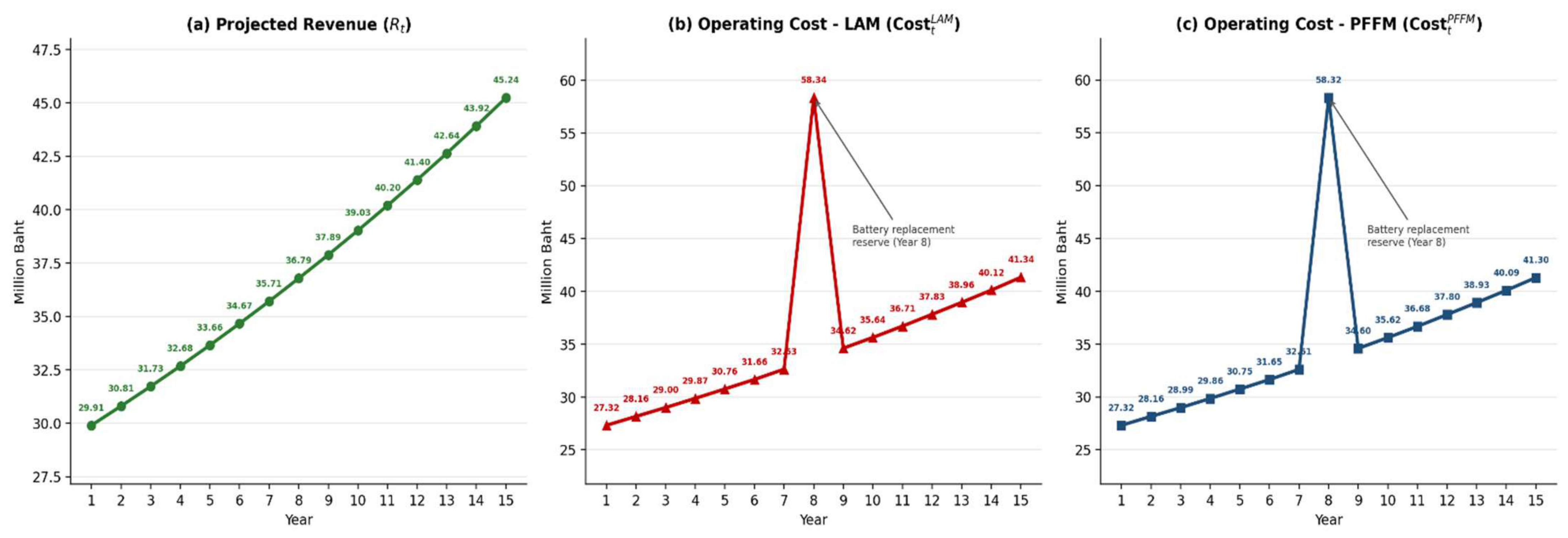
The comparative trends in revenue and operating costs under the PFFM and LAM over the 15-year project horizon are presented in Figure 5.

As illustrated in Figure 5, projected revenue increases steadily from THB 29.91 million in Year 1 to THB 45.24 million in Year 15. Under the Linear Assumption Model (LAM), operating costs increase from THB 27.32 million to THB 41.34 million, while the Production Function-Based Financial Feasibility Model (PFFM) produces marginally lower estimates, rising from THB 27.32 million to THB 41.30 million over the same period. In Year 8, operating costs increase sharply to THB 58.34 million under the LAM and THB 58.32 million under the PFFM due to the scheduled battery replacement expenditure. Consequently, operating costs exceed projected revenue of THB 36.79 million in that year. In all other years, projected revenue remains above operating costs, although the operating margins are relatively modest. The close correspondence between the two cost trajectories indicates that the PFFM adjustment produces only a marginal difference from the conventional linear-assumption approach.

4.2.3. Sensitivity Analysis of Energy-Price Changes (Worst-Case Scenario)

Electricity is the primary production input with a statistically significant coefficient of $\alpha =0.99025$. Therefore, the researchers tested the worst-case scenario by increasing the electricity price by 30% throughout the project life-cycle. This causes energy costs to increase proportionally, resulting in similar upward adjustments in both $AV{C}_{LAM}$ and $MC$ under the PFFM. The calculation results are presented in

Table 7. Sensitivity analysis results under a 30% increase in electricity price.

Scenario	Indicator	PFFM	LAM
A 30% increase in electricity price	NPV (million Baht)	−293.12	−293.26
	IRR (%)	Not attainable	Not attainable
	Payback period (year)	Not attained (>15 yrs)	Not attained (>15 yrs)

.

According to Table 6, the worst-case scenario further reduces NPV relative to the base case for both models (PFFM: from −271.61 to −293.12 million Baht; LAM: from −271.74 to −293.26 million Baht), a decline of approximately 21.5 million Baht attributable to the 30% electricity price increase. IRR and payback period remain unattainable within the 15-year horizon in both models under the worst-case scenario, consistent with the base-case result (Section 4.2.2). This confirms that the project’s financial infeasibility on a pure farebox and advertising revenue basis is robust to further adverse energy-price shocks, and that the PFFM continues to incur a marginally smaller loss than the LAM, consistent with its lower marginal cost structure. The energy-cost share used to derive the worst-case Cost_t series in this table was approximated from the Year 1 route-level data in Table 2 (electricity cost/total OPEX = 25%); researchers replicating this analysis should verify the exact figure against the underlying route-level cost model before final submission, since the energy-cost share may vary modestly across years and routes.

4.2.4. Net Present Value Gap Analysis

Based on Equation (6), the NPV gap under the base-case scenario is calculated as follows:

$$Ga{p}_{NPV}(\%)={\displaystyle \frac{NP{V}^{LAM}-NP{V}^{PFFM}}{\mid NP{V}^{PFFM}\mid }}\times 100={\displaystyle \frac{-271.74-(-271.61)}{271.61}}\times 100=-0.05\%$$

A $Ga{p}_{NPV}$ of approximately −0.05% indicates that, when cash flows are correctly specified without the erroneous depreciation add-back (Equation (4)), the LAM and PFFM models produce very similar results under the base-case scenario: both yield a significantly negative NPV, with their difference being negligible. This near-zero gap is, nonetheless, theoretically consistent with the estimated returns to scale of RTS = 1.0062—just slightly above 1—as both models tend to converge as RTS nears 1. The LAM, assuming RTS = 1 and FC = 0, and the PFFM, which estimates RTS from data, align their cost structures and valuation outcomes. They are likely to diverge more in projects with stronger increasing or decreasing returns to scale. This finding empirically confirms the internal theoretical consistency of the PFFM framework, rather than indicating a practically important valuation gap in the present case.

4.2.5. Summary of Analysis Results

Based on the estimated production function, a RTS value of 1.0062, which is greater than 1, indicates that the EV bus project demonstrates mild economies of scale. The PFFM, which incorporates this parameter to formulate fixed-cost and marginal cost assumptions, is structurally more suited to reflect the actual cost structure than the LAM, which assumes RTS = 1 and excludes fixed costs. Since RTS is very close to 1, the models’ results show only a negligible difference between the models ($Ga{p}_{NPV}$ = −0.05%). The greater analytical value of the PFFM here is not in producing a materially different estimate but in correctly showing, through Equation (4) and Table 5, that neither model indicates the project is financially self-sustaining based solely on farebox and advertising revenue (NPV^LAM = −271.74 million Baht; NPV^PFFM = −271.61 million Baht; Section 4.2.2). This indicates that the PFFM provides a theoretically consistent and transparent basis for assessing financial feasibility, with its practical differences from the LAM scales with the estimated returns to scale.

Therefore, this study supports the application of the PFFM framework by public agencies in the appraisal of public service projects, even when RTS is close to 1, because the PFFM provides a transparent and verifiable link between the estimated production technology and the resulting cost assumptions. This transparency is valuable independently of whether the PFFM and LAM produce numerically similar or different results in a given case: it allows analysts to attribute the source of any gap to the estimated production parameters (RTS, MC, FC) rather than to arbitrary modelling choices, and it correctly reveals, in the present case, that the EV bus project requires public service obligation (PSO) subsidy or additional revenue streams beyond farebox and advertising income to achieve financial sustainability (Section 4.2.2).

4.3. Synthesis of Financial Analysis Results into a Prototype PFFM Framework for Public Investment Projects

Based on the PFFM financial analysis presented in Section 4.1 and Section 4.2, together with policy discussions with EV bus project stakeholders, this study concludes that both the conventional linear assumption model (LAM) and the Cobb–Douglas-based PFFM (RTS = 1.0062, MC = 3.1945 Baht/km, and FC = 0.1667 million Baht/year) indicate that the project is financially infeasible on a farebox and advertising revenue basis: the base-case NPV is negative for both models (LAM: −271.74 million Baht; PFFM: −271.61 million Baht), and this result is robust to a worst-case 30% increase in electricity price (LAM: −293.26 million Baht; PFFM: −293.12 million Baht; Section 4.2.3). Because the estimated RTS is very close to 1, the PFFM and LAM produce closely converging valuations in this case ($Ga{p}_{NPV}$ = −0.05%), which is theoretically consistent rather than evidence against the PFFM’s usefulness. The practical contribution of the PFFM here is diagnostic rather than comparative: by correctly and transparently specifying project cash flows (Equation (4)), it reveals that the EV bus project is not self-financing under current revenue assumptions and that a public service obligation (PSO) subsidy, fare adjustment, or additional ancillary revenue (e.g., commercial leasing, carbon credits) would be required to achieve financial sustainability, consistent with the project’s own PSO-based policy assumptions (Section 2.1) and with international practice in urban public transport finance.

However, based on discussions at the meeting with relevant agencies, participants agreed that the PFFM approach should serve as a reference framework for designing a gross-cost bus operation contract covering all three routes under a single contract. It should also be used to support negotiations on Time-of-Use electricity tariffs and to plan charging during off-peak periods in order to reduce energy costs. A key recommendation is that the Provincial Administrative Organization maintain its role as the regulator by establishing strict KPIs, while ensuring that all fare revenues are transferred into the PAO system. This would help strengthen public confidence in the service system and support its long-term sustainability.

Finally, the PFFM is proposed as a prototype framework for other public service projects in developing countries, particularly projects characterised by fixed costs or returns to scale that differ from 1. This is because the model can reflect cost dynamics based on actual production technology and appropriately strengthen confidence in public investment decision-making. Even in cases where RTS is close to 1, the PFFM still provides benefits in terms of transparency, verifiability, and reduced systematic bias compared with the LAM.

4.4. Social Return on Investment (SROI) Analysis

The base-case and worst-case results reported in Section 4.2.2 and Section 4.2.3 indicate that, on a farebox and advertising revenue basis, neither the PFFM nor the LAM recovers its investment within the 15-year appraisal horizon (NPV^LAM = −271.74 million Baht; NPV^PRPM = −271.61 million Baht; IRR not attainable in either model). Applying the SROI formulation, baseline data, and benefit stream methodology presented in Section 3.4, this section reports the resulting monetised social benefit streams, net benefits, and SROI ratio for the project.

4.4.1. Estimated Social Benefit Streams

The seven monetised benefit streams described in Section 3.4.2 yield the annual Gross Benefits summarised in

Table 8. Estimated annual social benefit streams (Gross Benefits).

No.	Benefit Stream	Value (Million Baht/Year)
1	Net energy-cost savings	32.12
2	Net maintenance cost savings	17.48
3	Avoided health damage cost (PM2.5, NOx, CO)	7.07
4	Carbon credit value (GHG reduction)	1.44
5	Avoided accident cost	22.20
6	Reduced traffic congestion/time value	30.00
7	Local economic uplift	10.00
	Total Gross Benefits	120.31

Source: Compiled by the researchers based on the studies of Chantuk et al. (2026) and Carbone et al. (2025).

.

4.4.2. SROI Calculation and Interpretation

Applying Equation (8), net benefits are calculated as Gross Benefits (120.31 million Baht/year) × (1 − 0.05) × (1 − 0.05) × (1 − 0.00) = 108.58 million Baht/year. Relative to the project’s total annual cost of 31.46 million Baht/year (Chantuk et al., 2026), Equation (7) yields

SROI = 108.58 ÷ 31.46 = 3.45

An SROI of 3.45 indicates that every 1 Baht invested by the Khon Kaen Provincial Administrative Organization in the EV bus project generates approximately 3.45 Baht in social value. Decomposing the 120.31 million Baht in Gross Benefits (Table 8) shows that energy savings (26.4%) and reduced congestion/time loss (24.7%) together account for over half of total social value, followed by accident reduction (18.3%), maintenance savings (14.4%), local economic uplift (8.2%), avoided health damage (7.0%), and carbon credits (0.9%). Taken alongside Section 4.2.2, Section 4.2.3, Section 4.2.4, Section 4.2.5 and Section 4.3, this result indicates that the project is not commercially self-financing on a farebox and advertising revenue basis, yet generates social returns that substantially exceed its annual cost once environmental, health, safety, and time-saving externalities are monetised—a pattern consistent with the general public service obligation (PSO) rationale for subsidising urban public transport (European Commission, 2014). This finding is discussed further, alongside the limitations of the underlying deadweight, attribution, and monetisation assumptions, in Section 5.

5. Discussion

The findings of this study indicate that the linear assumption model (LAM), commonly used by public agencies in financial feasibility studies, has significant structural limitations. In particular, it assumes that revenues and costs grow at constant rates, without accounting for the enterprise’s actual production technology. As Walters (1963) noted, the cost structures of public transportation and utility enterprises are complex and non-linear. This study confirms that neglecting fixed costs and assuming constant returns to scale (RTS = 1) cause the LAM to overestimate net cash flows. Although the difference identified in this case study is relatively small, the bias direction is consistent with cases in which RTS differs significantly from 1. This finding is consistent with the argument of Blessing and Ifeanyi (2025), who suggested that parametric cost estimation often fails to consider market volatility and structural uncertainty, thereby leading to optimism bias in budgeting for infrastructure projects.

Additionally, considering the volatility of energy prices, which represents the primary production input of the EV bus project, the results show that the PFFM, which integrates the Cobb–Douglas production function and applies returns to scale (RTS) and marginal cost (MC) parameters, can systematically provide more conservative estimates and better reflect risk than the LAM. This is consistent with the concepts proposed by Massot (2014) and Terblanche and Root (2022), who stated that using production functions with cash flow estimation can improve accuracy and reliability because the results align with actual production technology. The LAM cannot effectively measure interactions among production inputs or changes in input prices. To reduce optimism bias, which is commonly found in infrastructure projects, studies in production economics have proposed using quantitative tools, such as Value-at-Risk (VaR), to assess economic losses under uncertainty in production inputs. Such tools enable decision-makers to visualise risk in monetary terms more clearly than relying solely on standard deviation (Siaplay et al., 2005). This approach is consistent with the PFFM mechanism, which emphasises early warning detection through production parameters. Empirical evidence from Vepsäläinen et al. (2018) confirms that the energy costs and demand charges of EV bus systems vary significantly according to operating timetables and the number of charging stations. This represents a non-linear cost structure that the LAM cannot capture, whereas the PFFM can capture such non-linearity through the RTS and MC parameters.

However, this finding helps fill a gap in the existing literature. Although numerous studies have applied production functions to investment analysis, such as the studies of Koval et al. (2018) and Massot (2014), as well as the study by Gumulya et al. (2020), which used the Cobb–Douglas function with internal variables of the Business Model Canvas (BMC) to analyse the relationships among key resources, cost structure, and revenue streams in basic and chemical industries, most of these studies have focused primarily on explaining business structures rather than conducting in-depth financial feasibility assessment. They have not explicitly compared systematic bias against the linear assumption model (LAM), particularly in the context of public transportation projects characterised by exogenously restricted output, as framed by Malikov et al. (2024). This study conducted and demonstrated that incorporating returns to scale and marginal cost into financial appraisal can reduce systematic bias, even when the RTS value is close to 1. This finding is consistent with the recommendation of Shim and Kim (2022), who argued that financial feasibility assessment in developing countries should place greater emphasis on production technology factors rather than relying on convenient but potentially inaccurate linear assumptions.

Comparing this study’s findings with previous studies in Thailand, Chiradjea et al. (2025) found that EV charging infrastructure projects in residential buildings require an 8 THB per kWh profit margin to break-even over a 20-year horizon, with a 14-year payback period and an internal rate of return of only 4.29%, which is below typical financing costs. In contrast, the Khon Kaen EV Bus project’s PFFM analysis shows a negative NPV of approximately −271.6 million Baht over 15 years on a farebox and advertising revenue basis (Section 4.2.2). Neither the PFFM nor the LAM recovers the initial investment within the appraisal horizon. However, the social return on investment (SROI) analysis in Section 4.4 indicates that, once unpriced externalities such as avoided air pollution, reduced accidents, and time savings are monetised, the project generates an SROI of 3.45, meaning that every 1 THB invested generates approximately 3.45 THB in social value. This discrepancy between a negative financial NPV and a strongly positive SROI highlights the limitations of purely financial metrics for evaluating public transportation projects and underscores the value of incorporating both production economics and social-value appraisal into the investment decision framework.

In the East Asian context, while China, South Korea, and Japan have made significant progress in EV bus deployment (Wang et al., 2024; Kim et al., 2021), prior studies in this region have focused primarily on engineering and operational aspects. None have integrated production function parameters into financial feasibility analysis. Our study thus contributes to the regional literature by demonstrating that, even when RTS is close to 1 (indicating approximately constant returns to scale), incorporating production parameters improves the transparency and consistency of financial appraisal and reduces systematic bias compared with the linear assumption model (LAM) commonly used in Thai feasibility studies.

In addition, the findings lead to implications for contract design and risk management planning in public-sector projects. The PFFM provides advanced financial evidence that can serve as a reference framework for negotiations with the private sector and for the design of gross-cost O&M contracts. This is consistent with the case studies of the Phuket Provincial Administrative Organization and the Kanchanaburi Provincial Administrative Organization, which emphasised the importance of separating vehicle leasing contracts from operation and management contracts, as well as adopting a model in which the public sector controls policy (Haass & Guzman, 2020). Therefore, the PFFM is not merely a financial calculation tool, but also serves as a framework for planning public–private management arrangements and supporting public investment decision-making, which is a key element in improving the standards of public investment project appraisal in developing countries, as suggested by Terblanche and Root (2024) and Blessing and Ifeanyi (2025).

5.1. Implications

This study advances the literature in three ways. First, it bridges production economics and project finance by demonstrating that returns to scale (RTS) and marginal cost (MC) can be systematically integrated into financial feasibility analysis. While prior studies in Thailand (Chiradjea et al., 2025) and the broader energy sector (Gómez-Restrepo et al., 2024) have relied on deterministic models (NPV, IRR, LCOE) that assume constant growth, the PFFM reveals that incorporating RTS and MC yields more conservative yet structurally accurate cash flow projections. This challenges the conventional linear assumption model (LAM) and demonstrates that even near-constant RTS (=1) masks critical cost dynamics. Second, the study provides empirical evidence from a developing-country context, where infrastructure projects exhibit high energy-price sensitivity and fixed-cost intensity; the finding that energy elasticity (α = 0.990) dominates the production function underscores energy-cost management as a critical success factor. Third, the study demonstrates the feasibility of calibrating production functions using projected operational data when historical data are unavailable, offering a practical template for researchers evaluating early-stage infrastructure projects in data-scarce environments.

5.2. Policy and Practical Implications

The PFFM offers a transparent decision-support tool for public-sector stakeholders. First, by explicitly deriving MC (3.19 THB/km) and FC (0.17 million THB/year), the model enables local administrative organisations to design performance-based O&M contracts with clear reference frameworks, mitigating information asymmetry in negotiations with private operators. Second, the model’s capacity to quantify downside risk under energy-price volatility, as demonstrated by the 30% electricity price shock scenario, provides a robust basis for establishing contingency reserves and determining subsidy thresholds. Third, the integration of social return on investment (SROI = 3.45:1) strengthens the case for public funding by translating externalities, including reduced PM2.5 emissions, improved road safety, and time savings, into monetised social returns, thereby enabling local governments to communicate project value to taxpayers and oversight bodies. Fourth, the finding that RTS = 1 suggests that increasing service frequency may yield marginal cost savings, providing empirical support for strategic fleet planning decisions, such as the Khon Kaen PAO’s transition from a mixed fleet to a uniform medium-bus fleet.

6. Recommendations

According to the results of the PFFM development and its application to the EV bus project of the Khon Kaen Provincial Administrative Organization, the researchers propose the following policy and practical recommendations for relevant agencies:

6.1. Policy Recommendations

(1)

Enhance public investment project appraisal standards. Relevant agencies should revise financial feasibility guidelines for public infrastructure projects characterised by high fixed costs. The updated guidelines should require the measurement of returns to scale and require marginal cost analysis based on actual production technology, utilising the PFFM assessment method rather than relying exclusively on the LAM. This strategy is expected to reduce bias and enhance the reliability of investment decisions.

(2)

Public–private partnership (PPP) contracts should be designed using actual cost data. Project-owning agencies are advised to utilise returns to scale (RTS) and marginal cost (MC) parameters derived from the PFFM as a reference framework when negotiating gross-cost operations and maintenance (O&M) contracts, especially in public transportation projects. This approach can help prevent asymmetric information and mitigate the risk of private operators submitting inflated price proposals.

(3)

The integration of the Production Function-Based Financial Feasibility Model (PFFM) with social return on investment (SROI) assessment is recommended. Local administrative organisations implementing electric vehicle (EV) bus projects should be encouraged to prepare SROI reports in conjunction with financial analyses using the PFFM. These assessments should utilise actual data from fleet management systems and passenger counters to substantiate the justification for public subsidies and to demonstrate the social benefits produced by the project. This study’s own SROI analysis (Section 4.4), based on projected rather than observed operating data, illustrates the approach; once the project is operational, local administrative organisations should replicate this assessment using actual fleet management and passenger-counter data to validate and update the estimated SROI.

6.2. Recommendations for Future Research

(1)

The application of the PFFM should be extended to additional types of public investment projects that exhibit high fixed costs and non-constant returns to scale, including rail-based mass transit systems, water management projects, and public hospitals. Such extensions would facilitate the assessment of the model’s generalisability and inform its refinement across diverse project contexts.

(2)

Integrating the PFFM with life-cycle cost analysis is recommended. Future research should connect the PFFM with models of battery degradation and electric bus service life to improve the accuracy of forecasting battery replacement and disposal costs. Such integration would enhance the comprehensiveness of financial feasibility assessments throughout the entire project life-cycle.

(3)

The PFFM should be developed as open-source software, either as a user-friendly spreadsheet, such as Microsoft Excel, or as an accessible software application. It should include a manual for adjusting parameters to reflect local contexts, including electricity tariffs, labour costs, and the social discount rate. Dissemination through an online platform would enable local administrative organisations to download, implement, and verify the tool. This approach would facilitate knowledge sharing and help reduce technical disparities among public agencies.

References

1. Albulescu, C. T. (2020). Investment behavior and firms’ financial performance: A comparative analysis using firm-level data from the wine industry. International Journal of Management, Knowledge and Learning, 9(1), 75–94. [Google Scholar] [CrossRef] [Scilit]
2. Andreolli, F., D’Alpaos, C., & Moretto, M. (2022). Valuing investments in domestic PV-battery systems under uncertainty. Energy Economics, 106, 105721. [Google Scholar] [CrossRef] [Scilit]
3. Benchimol, J. (2015). Money in the production function: A new Keynesian DSGE perspective. Southern Economic Journal, 82(1), 152–184. [Google Scholar] [CrossRef] [Scilit]
4. Blessing, A. C., & Ifeanyi, O. E. (2025). Cost estimation and analysis for better project budgeting. Journal of Engineering Research and Reports, 27(7), 418–426. [Google Scholar] [CrossRef] [Scilit]
5. Booth, L. (1991). The influence of production technology on risk and the cost of capital. The Journal of Financial and Quantitative Analysis, 26(1), 109–127. [Google Scholar] [CrossRef] [Scilit]
6. Boratyński, J., & Osiewalski, J. (2021). Bayesian estimation of capital stock and depreciation in the production function framework. Central European Journal of Economic Modelling and Econometrics, 13(4), 455–486. [Google Scholar] [CrossRef]
7. Carbone, C., Sanzo, N., Dorsini, R., Nigliaccio, G., Di Florio, G., Cigolotti, V., & Agostini, A. (2025). An economic and environmental assessment of different bus powertrain technologies in public transportation. Cleaner Environmental Systems, 16, 100250. [Google Scholar] [CrossRef] [Scilit]
8. Cartenì, A. (2018). A cost-benefit analysis based on the carbon footprint derived from plug-in hybrid electric buses for urban public transport services. WSEAS Transactions on Environment and Development, 14, 125–135. [Google Scholar]
9. Chantuk, T. (2016). An analysis marginal cost and marginal revenue for services apartment boutique hotel feasibility. Modern Management Journal, 9(3), 79–95. [Google Scholar]
10. Chantuk, T., Inthawee, T., Pichaibhat, S., Tongmar, T., & Limarunothai, W. (2026). Final report: Feasibility study of electric bus (EV Bus) service on routes in Mueang Khon Kaen District for public service and air pollution reduction in Khon Kaen Province (Contract No. 1/2025). Academic Services Office, Silpakorn University. [Google Scholar]
11. Chiradjea, P., Yodphet, S., Sottyapahi, C., Kloaksing, C., Ananwattanaporn, S., & Ngaopitakkul, A. (2025). Analysis of investment feasibility for EV charging stations in high-density residential buildings: Empirical evidence from Thailand. IEEE Access, 13, 33985–33994. [Google Scholar]
12. Christensen, L. R., Jorgenson, D. W., & Lau, L. J. (1973). Transcendental logarithmic production frontiers. The Review of Economics and Statistics, 55(1), 28–45. [Google Scholar] [CrossRef] [Scilit]
13. Chritamara, S. (2017). An application of the real option framework to large infrastructure projects: Evidence for Thailand’s transportation system [Doctoral dissertation, Newcastle University]. [Google Scholar]
14. Cobb, C. W., & Douglas, P. H. (1928). A theory of production. American Economic Review, 18(1), 139–165. [Google Scholar]
15. Corvo, L., Pastore, L., Mastrodascio, M., & Cepiku, D. (2022). The social return on investment model: A systematic literature review. Meditari Accountancy Research, 30(7), 49–86. [Google Scholar] [CrossRef] [Scilit]
16. Dai, W., & Zhou, X. (2011). Feasibility of establishing an industrial investment fund in Jiangsu coastal area: Based on Cobb-Douglas production function and GM (1,1) prediction model. In 2011 international conference of information technology, computer engineering and management sciences (pp. 53–56). IEEE. [Google Scholar] [CrossRef] [Scilit]
17. Dydkowski, G., Gnap, J., & Urbanek, A. (2021). Electrification of public transport bus fleet: Identification of business and financing models. Communications—Scientific Letters of the University of Zilina, 23(3), A137–A149. [Google Scholar] [CrossRef] [Scilit]
18. European Commission. (2014). Guide to cost-benefit analysis of investment projects. Directorate-General for Regional and Urban Policy. [Google Scholar]
19. Fabianová, J., & Janeková, J. (2022). Economic assessment of investment in electric buses and CNG buses—A case study of a public transport company. Advances in Science and Technology Research Journal, 16(4), 96–105. [Google Scholar] [CrossRef] [Scilit] [PubMed]
20. Fahrizal, F., Jasman, J., Nggadung, Y., & Kartiwan, K. (2020). Optimisation production model and financial feasibility analysis on planning of integrated lontar sugar industry in Rote Ndao, East Nusa Tenggara, Indonesia. Tropical Drylands, 4(1), 25–30. [Google Scholar] [CrossRef] [Scilit]
21. Felipe, J., & Adams, F. G. (2005). The estimation of the Cobb-Douglas function: A retrospective view. Eastern Economic Journal, 31(3), 427–445. [Google Scholar]
22. Gordon, D., & Vaughan, R. (2011). The historical role of the production function in economics and business. American Journal of Business Education, 4(4), 25–30. [Google Scholar] [CrossRef] [Scilit]
23. Gómez-Restrepo, A. M., González-Ruiz, J. D., & Botero-Botero, S. (2024). Financial investment valuation models for photovoltaic and energy storage projects: Trends and challenges. Energies, 17(11), 2653. [Google Scholar] [CrossRef] [Scilit]
24. Grauers, A., Borén, S., & Enerbäck, O. (2020). Total cost of ownership model and significant cost parameters for the design of electric bus systems. Energies, 13(12), 3262. [Google Scholar] [CrossRef] [Scilit]
25. Gumulya, D., Sutikno, H., Pramono, R., & Hariandja, E. S. (2020). Regression analysis of inter-variable relationships within business canvas model: Value proposition, key resources, revenue and cost structure with the Cobb Douglass production function approach (Study case: Basic and chemical industries from 2006–2017). Jurnal Manajemen Indonesia, 20(2), 96–113. [Google Scholar] [CrossRef] [Scilit]
26. Haass, O., & Guzman, G. (2020). Understanding project evaluation—A review and reconceptualisation. International Journal of Managing Projects in Business, 13(3), 573–599. [Google Scholar] [CrossRef] [Scilit]
27. Hasugian, I. A., Dewi, E., & Vandrick. (2020). Engineering economics evaluation for manufacturing competitiveness: A case study. IOP Conference Series: Materials Science and Engineering, 851(1), 012027. [Google Scholar] [CrossRef] [Scilit]
28. Ikonnikova, S. A., del Carpio Neyra, V., & Berdysheva, S. (2022). Investment choices and production dynamics: The role of price expectations, financial deficit, and production constraints. Journal of Economics and Business, 120, 106067. [Google Scholar] [CrossRef] [Scilit]
29. Jedwanna, K., & Pongthanaisawan, J. (2021). Cost-benefit analysis of alternative vehicle technologies for the urban bus system in Thailand. Journal of Research and Innovation Rajamangala University of Technology Krungthep, 15(1), 1–16. [Google Scholar]
30. Karimova, S. U. (2026). Assessment of investment efficiency based on industrial production growth rates and investment dynamics. International Scientific-Electronic Journal “Pioneering Studies and Theories”, 2(1), 82–90. [Google Scholar]
31. Kim, K., Kim, J., & Yook, D. (2021). Analysis of features affecting the contracted rate of return of Korean PPP projects. Sustainability, 13(6), 3311. [Google Scholar] [CrossRef] [Scilit]
32. Kongwee, W., Achariyaviriya, W., Rinchumphu, D., Suttakul, P., & Achariyaviriya, A. (2025). Spatial analysis of EV charging demand for intercity bus transport in Thailand. IISPRS Annals of the Photogrammetry, Remote Sensing and Spatial Information Sciences, X-4/W7-2025, 83–88. [Google Scholar] [CrossRef] [Scilit]
33. Koval, V., Slobodianiuk, O., & Yankovyi, V. (2018). Production forecasting and evaluation of investments using Allen two-factor production function. Baltic Journal of Economic Studies, 4(1), 219–226. [Google Scholar] [CrossRef] [Scilit]
34. Land Transport Authority. (2023). Electric bus trial and deployment plan. Land Transport Authority.
35. Li, L., & Cao, X. (2022). Comprehensive effectiveness assessment of energy storage incentive mechanisms for PV-ESS projects based on compound real options. Energy, 239, 121902. [Google Scholar] [CrossRef] [Scilit]
36. Lotfi, M., Pereira, P., Paterakis, N. G., Gabbar, H. A., & Catalão, J. P. S. (2020). Optimal design of electric bus transport systems with minimal total ownership cost. IEEE Access, 8, 119184–119199. [Google Scholar] [CrossRef] [Scilit]
37. Malikov, E., Zhao, S., Kumbhakar, S. C., & Bernstein, D. H. (2024). Estimating production functions using costs when outputs are restricted. Econometric Reviews, 44(4), 433–461. [Google Scholar] [CrossRef] [Scilit]
38. Martini, D., Bezzini, P., & Longo, M. (2024). Environmental impact of electrification on local public transport: Preliminary study. Energies, 17(20), 5886. [Google Scholar] [CrossRef] [Scilit]
39. Massot, J. M. (2014). Financial evaluation of long-term investments: The role of explicit production functions. European Scientific Journal, 1, 457–468. [Google Scholar]
40. Muhamed, A. A., Leuveano, A. C., Zakariah, H., Bakar, M. Z. A., & Halif, M. M. (2023). Integrating economic and environmental factors: A decision model framework for supply chain development. International Journal of Academic Research in Business and Social Sciences, 13(6), 1390–1398. [Google Scholar] [CrossRef] [Scilit] [PubMed]
41. Nicholls, J., Lawlor, E., Neitzert, E., & Goodspeed, T. (2012). A guide to social return on investment. The SROI Network. [Google Scholar]
42. Pei, Y., Guo, M., Zhang, J., & Peng, K. (2024). Can the development of electric buses bring economic and environmental benefits. Advances in Economics and Management Research, 9, 241–250. [Google Scholar] [CrossRef] [Scilit]
43. Prapaporn, W., Inohae, T., Kaewwichian, P., & Siewwuttanagul, S. (2022). Feeder bus reformation for an urban rail project: The case of Khon Kaen city, Thailand. Journal of Regional and City Planning, 33(2), 227–243. [Google Scholar] [CrossRef] [Scilit]
44. Rezepin, A., Amirova, T., & Mishina, V. (2017). The research of the production function of an industrial enterprise. SHS Web of Conferences, 35, 01038. [Google Scholar] [CrossRef] [Scilit]
45. Saelee, C. (2021). Cost and sensitivity analysis of investment project in cleaning service business: Case study of Me D Property Service Management Company Limited. Business Administration and Economics Review, 17(1), 40–56. [Google Scholar]
46. Shim, H. C., & Kim, J. H. (2022). Determinants of the economic and financial feasibility of development projects: A comparative analysis between public and private development projects in South Korea. Sustainability, 14(4), 2135. [Google Scholar] [CrossRef] [Scilit]
47. Siaplay, M., Nganje, W., & Kaitibie, S. (2005). Value-at-risk and food safety losses in turkey processing (Agribusiness & Applied Economics Report No. 557). Department of Agribusiness and Applied Economics, North Dakota State University. Available online: http://ageconsearch.umn.edu (accessed on 5 July 2026).
48. Stadtherr, F., & Wouters, M. (2021). Extending target costing to include targets for R&D costs and production investments for a modular product portfolio—A case study. International Journal of Production Economics, 231, 107871. [Google Scholar] [CrossRef] [Scilit]
49. Tantiwat, W. (2025). Investigating the transportation economics of the Eastern Economic Corridor in Thailand. Journal of Applied Economics and Management Strategy, 12(1), 277–296. [Google Scholar] [CrossRef] [Scilit]
50. Terblanche, R., & Root, D. S. (2022). Evaluating financial feasibility studies based on real estate developers’ requirements. Journal of Applied Business and Economics, 24(5), 194–203. [Google Scholar] [CrossRef] [Scilit]
51. Terblanche, R., & Root, D. S. (2024). Consolidating the roles of financial feasibility studies: Property developers vs quantity surveyors. Organization, Technology and Management in Construction, 16, 136–149. [Google Scholar] [CrossRef] [Scilit]
52. Thailand Greenhouse Gas Management Organization (TGO). (2023). Emission factors for Thailand grid & transport. TGO.
53. Vepsäläinen, J., Baldi, F., Lajunen, A., Kivekäs, K., & Tammi, K. (2018). Cost-benefit analysis of electric bus fleet with various operation intervals. In 2018 21st international conference on intelligent transportation systems (ITSC) (pp. 1522–1527). IEEE. [Google Scholar] [CrossRef] [Scilit]
54. Vijay, U., Woo, S., Moura, S. J., Jain, A., Rodriguez, D., Gambacorta, S., Ferrara, G., Lanuzza, L., Zulberti, C., Mellekas, E., & Papa, C. (2023). Valuation of urban public bus electrification with open data and physics-informed machine learning. Journal of Advanced Transportation, 2023, 5021883. [Google Scholar] [CrossRef] [Scilit]
55. Walters, A. A. (1963). Production and cost functions: An econometric survey. Econometrica, 31(1/2), 1–66. [Google Scholar] [CrossRef] [Scilit]
56. Wang, G., Zhao, Y., Pan, Y., & Shi, T. (2024). Integrated optimization study of electric bus fleet transformation: Based on LCA, LCC and multi-objective planning. Academic Journal of Science and Technology, 11(2), 1–7. [Google Scholar] [CrossRef] [Scilit]
Figure 1. Proposed EV bus routes in Mueang Khon Kaen District. Route 1 (Purple) connects Ban Ped to Ban Kok Si via Sri Chan Road. Route 2 (Pink) links Bus Terminal 3 to Ban Samran via Mittraphap Road and Khon Kaen University. Route 3 (Brown) connects Ban Ped to the airport and Prachasamosorn Road.
Jrfm 19 00560 g001
Figure 2. Research conceptual framework of the PFFM integrating the Cobb–Douglas production function and linking financial feasibility analysis with SROI assessment.
Jrfm 19 00560 g002
Figure 3. CAPEX investment breakdown by category for the EV bus project of Khon Kaen Provincial Administrative Organization (Total = THB 285.05 million). Source: Table 1.
Jrfm 19 00560 g003
Figure 4. Eenergy-cost ( E t × p E ) trend over the 15-year project life-cycle.
Jrfm 19 00560 g004
Figure 5. Projected revenue and operating cost trends, PFFM vs. LAM (Years 1–15). Source: Table 5.
Jrfm 19 00560 g005