Deep Learning in Credit Risk Assessment: A Data-Driven Approach to Transforming Financial Decision-Making and Risk Analytics

Abstract

Credit risk evaluation is a key factor in financial intermediation, regulatory capital provision, and risk management in the portfolio. In this study, we compare the deep learning performance for probability-of-default (PD) estimation with a structured financial econometric model using loan-level data of an Indian non-banking financial agency between May and August 2025. Using the interpretation of PD as a conditional expectation, which is in line with reduced-form default-intensity models, we compare deep learning, logistic regression, and gradient boosting using a pure time-based out-of-sample design. Model assessment focuses on discrimination and calibration, where the area under the precision–recall curve (AUC-PR), Brier score, log-loss, and Hosmer–Lemeshow goodness-of-fit tests are utilized. The findings show that deep learning achieves higher accuracy in terms of calibration but a lower Brier score by about 18; this gap could be reduced by comparing logistic regression with statistically significant improvements in formal tests that compare forecasts. In portfolio back-testing, better probability scaling is translated into an actual loss reduction of about 12–13% for the August 2025 cohort. Although the improvements compared with the advanced ensemble techniques are moderate, the results indicate that deep learning improves the estimation of conditional default probabilities because of the better nonlinear modeling and upper-tail risk perception. This study contributes to the literature via its incorporation of machine learning and credit risk assessment into a formalized risk management and econometric assessment system.

1. Introduction

Modern financial intermediation, portfolio allocation, and capital regulation determination are all examples of credit risk assessments. These types of assessments are based on the estimation of the probability of default (PD), which is the conditional likelihood of a default (i.e., a failure of a borrower to fulfill their contractual duties within a determined horizon). In the context of a structural and reduced-form credit risk model, PD is not only the result of classification but also a conditional expectation accounted for when making decisions regarding asset pricing and risk management. In structural models, default is created when the value of a firm’s assets drops below the liability threshold (Merton, 1974; Black & Cox, 1976). In reduced-form models, the default model is a stochastic intensity process, where observable information is given (Jarrow & Turnbull, 1995; Cochrane, 2009; Duffie & Singleton, 2003). In both formulations, the correct modeling of PD has a direct impact on the modeling of expected loss, capital requirements, and risk in a portfolio.

The expected loss of a credit exposure is commonly expressed as follows:

EL = PD × LGD × EAD

Regulatory regimes like Basel II and Basel III incorporate probability-of-default (PD) estimates into capital calculations, which, in turn, hint at bad estimates of PD, significantly misallocating both economic and regulatory capital. Therefore, improvements in PD estimation are to be evaluated not only with the help of discrimination metrics but also by calibration accuracy and economic value.

Recent developments in machine learning, specifically deep learning models, have resulted in interest in their use for credit risk modeling. Neural networks, as well as other nonlinear methods, have the potential to model intricate interactions among borrower qualities, macroeconomic variables, and historical performance variables. Empirical studies often achieve improvements in the area under the receiver operating characteristic (AUC) or classification accuracy. However, much of the available literature that assesses models using random cross-validation places more emphasis on accuracy measures and often does not address calibration, statistical forecast comparison, or economic implications. Financially, an econometric point of view may overstate the predictive ability to uncover the economic significance of modeling gains, which obscures such evaluation strategies.

The current research is driven by two theoretical concerns. First, the problem with PD estimation is that its forecasting is time-dependent. Intersecting random data splits, which intermix both past and future data, can cause look-ahead bias and inflate out-of-sample quantities. Therefore, a time-consistent validation system is necessary. Second, an improvement in discrimination does not necessarily mean an improvement in risk measurement. A well-modeled ranking of borrowers can still generate poorly calibrated PD estimates, leaving an expected loss forecast and resulting in an inefficient portfolio decision being made. Proper scoring rules and a formal statistical forecast-comparison test are needed in order to determine whether the improvements are economically significant.

In this study, deep learning models are considered when evaluating credit risk in a structured financial econometric model. PD is treated as a conditional expectation that is consistent with reduced-form default-intensity models, and deep learning estimators are compared with benchmark logistic specifications in an out-of-sample design that is strictly time-based. The accuracy of the model is evaluated through discrimination metrics (e.g., the area under the precision–recall curve (AUC-PR)) and calibration metrics (e.g., the Brier score, log-loss, and the calibration slope). To address the problem of statistical significance, we use forecast-comparison procedures in accordance with the Diebold–Mariano framework and the Superior Predictive Ability test. Lastly, we also connect predictive performance to the economic results using the expected-loss backtest.

The research question is as follows: Are deep learning models economically significant in the estimation of PD relative to established econometric benchmarks? In particular, we test whether nonlinear architectures have better (i) out-of-sample discrimination, (ii) PD calibration, and (iii) expected loss forecasting and whether these are statistically significant and economically meaningful. The contribution of this study is threefold: to begin with, we entrench deep learning-based credit risk modeling within a consistent financial risk-management framework. Second, we use a time-based validation procedure, which reduces look-ahead bias. Third, we relate predictive gains to anticipated loss results to measure the economic worth of modeling complexity. The remainder of this study is organized as follows: Section 2 presents a literature review of structural and reduced-form default modeling and recent machine learning applications in credit risk. Section 3 outlines the econometric model and assessment procedure. Section 4 entails data and sample construction. Section 5 presents the backtest and test results. The robustness analysis and interpretability assessment can be found in Section 6. Finally, Section 7 concludes this study.

2. Literature Review

It is important to note that credit risk modeling has developed in three general streams of research: structural default models, reduced-form intensity models, and data-driven statistical learning methods. These strands vary in methodology but have the shared goal of estimating the conditional probability of default and measuring what the possibility of default means for valuation and risk management.

2.1. Structural Models of Two Events

The structural approach has its roots in the contingent claims model of Merton (1974), where default occurs when the value of a firm’s assets is less than the face value of its liabilities upon maturity. The meaning of equity in this context is taken to be a call option on firm assets, and the probability of default is calculated based on the distribution of the asset’s value implied by market information. Extensions of the Black and Cox (1976) model include an early default with barrier features, in which the default could take place before maturity if the asset’s value fell below a barrier level.

Structural model empirical studies tend to use equity prices and balance sheet data to estimate unobservable asset values (e.g., Bharath & Shumway, 2008). Despite the simplicity of the relationship between default and firm value dynamics that structural models give, there are powerful assumptions of capital structure, asset volatility, and market completeness. In addition, they have limited their practical application to retail or consumer credit portfolios, where there are no market-based asset values.

However, structural models have an influential conceptual standard: probability-of-default measures economic fundamentals and is implicit in the relationship of asset prices. Any empirical estimation of the PD method should thus be in line with economically significant sources of credit risk. Reduced-form and intensity-based models are reduced-form models that are differentiated by their reduction levels.

2.2. Models Distinguished by Degrees of Reduction

Reduced-form models take another approach where they see default as the coming of a stochastic event which is controlled by a conditional intensity process. According to Jarrow and Turnbull (1995) and Duffie and Singleton (2003), default is of rate λt, and this can be related to observable covariates and latent influences. It can be said that the conditional probability of default in a finite horizon is a function of integrated intensity when it is seen in this framework.

As an empirical approach to discrete-time hazard, logistic specifications or probit specifications are often employed to model the probability of default as a nonlinear function of borrower characteristics and macroeconomic variables (Chava & Jarrow, 2004). In this way, logistic regression may be viewed as a parametric approximation of the conditional default intensity. The benefit of reduced-form methods is their flexibility and the ability of risk drivers that can be observed without modeling asset values.

These approaches are also consistent with foundational investment science and portfolio optimization principles (Luenberger, 1998). Probability-of-default estimation is therefore a conditional expectation problem, as finding a probability-of-default, given the information set Ft, is the expected value of a default indicator. This interpretation drives the evaluation mechanisms of using the correct scoring rules and predictions of forecast tests as opposed to metrics that are classification-focused.

2.3. Classical Credit-Scoring and Statistical Benchmarks

From a broader statistical learning perspective, these approaches are closely related to classical machine learning frameworks (Hastie et al., 2009). Conventional credit-scoring models are mainly linear or generalized linear, in the most common case, logistic regression. Since the first discriminant analysis methods, like Altman (1968), and later logistic-based models commonly used in banking practice, they have provided a sense of interpretability and more robust calibration performance. Logistic regression induces a linear index of covariates, which in turn guarantees monotonic predictor–default probability relationships.

In credit-score-related applications, comparative studies compared an array of classification algorithms and have found an improvement in the performance of ensemble models such as random forests (Breiman, 2001) and gradient boosting machines (Friedman, 2001). However, some benchmarking research is based on random cross-validation splits and focused on the area under the receiver operating characteristic curve (AUC-ROC), and thus it devotes little attention to calibration or economic analysis.

Claims of predictive superiority require strenuous statistical testing and a meticulously constructed out-of-sample design (as highlighted in the literature on financial econometrics, e.g., Diebold & Mariano, 1995; White, 2000; Hansen, 2005). Unless these controls are provided, apparent improvements in discrimination may be due to overfitting or data snooping instead of improvements in forecasting.

2.4. Machine Learning and Deep Learning in Credit Risk

Recent developments in financial machine learning further emphasize feature engineering and model robustness in high-dimensional settings (Lopez de Prado, 2018), leading to nonlinear function approximators, which can effectively emulate complex interactions between attributes of borrowers. Deep multilayer neural networks can be used to represent high-dimensional general nonlinear dependencies flexibly. When used in credit risk modeling, larger AUC values are often achieved compared with those achieved using logistic benchmarks.

Although these developments have been made, there are a number of constraints in the available literature. To begin with, the evaluation usually focuses on classification accuracy rather than the calibration quality, which is essential for capital allocation and expected loss computation. Second, most studies fail to use time-consistent validation and thus face the risk of look-ahead bias. Third, the statistical significance of performance gains is rarely tested using the existing forecast-comparison techniques. Lastly, not many studies directly relate predictive improvement to economic performance, like expected loss or portfolio performance.

Risk-wise, the question is not how deep learning can be used to increase classification measures, but rather how the approach can be used to increase the estimation of conditional default probabilities in a way that is consistent and statistically and economically significant.

2.5. Positioning of the Present Study

This study contributes to the literature by employing deep learning credit risk models in a rigorous financial–economic framework. Specifically, we achieve the following:

Perform PD estimation interpretation contingent on reduced-form intensity models.

• Adopt a time-based out-of-sample design that maintains the time dependence of credit risk.
• Measure performance based on discrimination and calibration measures, with special attention paid to appropriate scoring rules.
• Make formal statistical forecast comparison tests to test predictive superiority.
• Relate modeling performance with anticipated loss forecasting with economic implications.

Through combining machine learning techniques with the already known principles of financial forecasting and risk assessment, this study aims to offer a stricter evaluation of deep learning applicability in credit risk assessment.

2.6. New Developments in Machine Learning and Explainable AI in Credit Risk

The integration of sophisticated machine learning methods with explainability models has seen growing importance in recent credit risk modeling research. Studies such as that by Chang et al. (2024) have shown that ensemble and deep learning models are more effective for forecasting credit default than traditional statistical methods, particularly high-dimensional models. Similarly, recent studies demonstrate that the use of tree-based models, such as random forests, is stable in terms of predictive performance and advantageous in terms of interpretability by offering post hoc methods. More broadly, interpretable machine learning frameworks emphasize transparency and model accountability (Molnar, 2022).

Recently, researchers have been interested in Explainable Artificial Intelligence (XAI) to overcome the black-box nature of machine learning models. For example, recent studies emphasize the relevance of SHAP-based solutions to enhance the soundness and credibility of feature attribution in credit risk models. Similarly, recent studies also highlight that explainability methods such as SHAP or LIME increase transparency, regulatory adherence, and trust in automated lending systems. In contrast, recent surveys highlight the growing importance of explainability in black-box models (Guidotti et al., 2018).

More recent work (2025) has gone further to combine predictive performance and interpretability. Ensemble models with SHAP explanations can exhibit greatly enhanced predictive accuracy as well as decision transparency in retail lending. Likewise, explainable AI systems based on gradient boosting and neural networks have been demonstrated to strike the right balance between performance and interpretability of models and thus are appropriate in a regulatory setting. SHAP (Shapley Additive Explanations) provides a theoretically grounded framework for attributing feature importance (Lundberg & Lee, 2017).

In addition, recent surveys point out that a current major issue in credit risk modeling is not only enhancing predictive power but also keeping models understandable, equitable, and stable under economic circumstances. These trends are a sign of a move beyond accuracy-focused modeling to economically useful, interpretable, and regulation-compliant machine learning systems. Recent studies published in financial risk journals also highlight the interaction between credit risk and market variables in complex environments (Tsuruta, 2024).

3. Econometric Framework

This subsection makes probability-of-default estimation a conditional forecasting issue and defines the benchmark estimator and the deep learning estimator being compared in this study. We then describe the performance measures and statistical comparison steps that we used.

3.1. Probability-of-Default as a Conditional Expectation

Y_i,t + 1 ∈ {0,1} are indicator variables that take a value of 0,1, i.e., 1 gives the indication that the borrower is defaulting within the horizon (t,t + 1) and 0 gives the indication that the borrower is not defaulting within the horizon (t,t + 1). This set of information, known as time t, is defined as the information set of borrower characteristics, past performance, and macroeconomic variables, denoted by F_t.

Probability of default (PD) is the conditional expectation of the default event.

PD_i,t = E [Y_i,t + 1|F_t]

In a reduced-form model, the formulation is an approximation of a default-intensity model in which the conditional hazard rate is determined by observable covariates, in the time-discretized form. In turn, the process of estimating the probability distribution of PD_i,t should be viewed not as a standard classification task but a nonlinear regression problem.

In the case of a portfolio of exposures that are indexed by the index i 1, 2, 3, …N, the expected loss at time t is as follows:

$${\mathbf{EL}}_{\mathbf{t}}\mathbf{=}{\sum }_{\mathit{i}\mathbf{=}\mathbf{1}}^{\mathit{N}}{\mathit{P}\mathit{D}}_{\mathbf{i}\mathbf{,}\mathbf{t}}\mathbf{\times }{\mathbf{LGD}}_{\mathbf{i}\mathbf{,}\mathbf{t}}\mathbf{\times }{\mathbf{EAD}}_{\mathbf{i}\mathbf{,}\mathbf{t}}$$

Since the processes of capital and provisioning directly depend on the variable PD_i,t, it is clear that the economic importance of both the discriminative and calibration accuracies is realized.

3.2. Benchmark Logistic Specification

The econometric model used is logistic regression. The covariate vector is denoted as X_i,t ∈ R_k. The model of logistics is given as follows:

$${\mathrm{PD}}_{\mathrm{i},\mathrm{t}}=\Lambda \left({{\mathrm{X}}^{\prime }}_{\mathrm{i},\mathrm{t}}\mathsf{\beta }\right)=\exp \left({{\mathrm{X}}^{\prime }}_{\mathrm{i},\mathrm{t}}\mathsf{\beta }\right)/1 + \exp \left({{\mathrm{X}}^{\prime }}_{\mathrm{i},\mathrm{t}}\mathsf{\beta }\right)$$

The logistic link function Λ(·) is used, and the parameter vector is estimated using maximum likelihood, defending the parameter vector β.

The logistic specification provides a linear-index structure and monotonic marginal effects; the structure is interpretable, and it provides calibration and performance in general. However, its limitations are its interactions and nonlinearities, except when modeling.

Another way to fortify the benchmark is to instead use a penalized (ridge) logistic form, which minimizes the regularized version.

L(β) − λ|β|²,

where L(β) is the log-likelihood and λ is a regularization parameter selected via validation.

3.3. Deep Learning Estimator

Deep learning systems learn the conditional expectation via a nonlinear mapping, which is flexible.

PD_i,t = f_θ(X_i,t),

The mapping f_θ is represented by a multilayer neural network with a parameter, which is represented by a weight tensor denoted as theta. It is possible to express a feed-forward architecture with several hidden layers L, expressed recursively as shown

h_(l) = σ(W_(l)h_(l−1) + b_(l)), l = 1, …, L,

with h(0) = X_i,t denoting the activation function and σ(·) representing the output layer

PD_i,t = Λ(W_(L+1)h_(L) + b_(L+1)).

The network is trained by minimizing the binary cross-entropy loss function.

L_(θ) = −∑_i,t[Y_i,t + 1log(PD_i,t) + (1 − Y_i,t+1)log(1 − PD_i,t)].

Deep learning is easier than logistic regression in that it removes the linear-index constraint that is present in a functional-approximation view.

In order to increase reproducibility and methodological transparency, we present the specification of the deep learning model to estimate the probability of default (PD) in detail. The model is realized in the form of a feed-forward multilayer neural network, which estimates the conditional expectation:

PD_i,t = f_θ(X_i,t)

where f is a nonlinear mapping of network weights.

3.3.1. Network Architecture

The neural network is composed of an input layer, which is related to the feature vector X_i,t.

There are three concealed layers with the following specifications:

• Layer 1: 64 neurons;
• Layer 2: 32 neurons;
• Layer 3: 16 neurons.

Output layer: one neuron that is the predicted probability of default.

3.3.2. Activation Functions

• Hidden layers: Rectified Linear Unit (ReLU);
• Output layer: Sigmoid function, which ensures that the predictions are in the range (0,1).

3.3.3. Optimization and Loss Function

• Optimizer: Adam;
• Learning rate: 0.001.

Loss: Binary cross-entropy, which is defined as:

L(θ) = −∑_i,t[Y_i,t + 1log(PD_i,t) + (1 − Y_i,t + 1)log(1 − PD_i,t)]

3.3.4. Regularization Techniques

To mitigate overfitting:

• Dropout: 0.2 implemented at the end of every hidden layer.
• Early stopping: the training was terminated when there was no improvement in validation loss in five consecutive epochs of the training.

L2 regularization: λ = 0.001.

3.3.5. Training Protocol

• Batch size: 256;
• Maximum epochs: 100.

Validation dataset: July 2025 sample to tune hyperparameters and early stop.

• Preprocessing of features: Standardization (zero mean, unit variance).

This architecture strikes a balance between flexibility and generalization performance, especially when nonlinear relationships and moderate class imbalance exist in credit risk data.

To enable an easy comparison of the modeling techniques adopted in this paper, we summarize the major specifications and hyper parameters of all benchmark and proposed models. These cover both standard econometric models like logistic and ridge regression, and the machine learning models, such as the random forest, gradient boosting, and the proposed deep learning architecture. The differences in model structure, estimation procedures, and tuning parameters, which are crucial in the provision of a consistent and reproducible empirical framework, are highlighted in the table.

Table 1. Model Hyperparameter Specification.

Model	Hyperparameters
Logistic Regression	No regularization; coefficients estimated via maximum likelihood
Ridge Logistic Regression	L2 regularization (λ selected via validation grid search)
Random Forest	Number of trees = 200; maximum depth = 6; bootstrap sampling enabled
Gradient Boosting	Number of estimators = 300; learning rate = 0.05; maximum depth = 3
Deep Learning (Proposed Model)	Architecture: 3 hidden layers (64–32–16 neurons) Activation: ReLU (hidden layers), Sigmoid (output layer) Optimizer: Adam (learning rate = 0.001) Loss Function: Binary cross-entropy Regularization: Dropout = 0.2; L2 penalty (λ = 0.001) Training Parameters: Batch size = 256; epochs = 100; early stopping = 5 epochs (validation-based) Preprocessing: Feature standardization (zero mean, unit variance)

summarizes the model specifications.

3.4. Performance Metrics

The test focuses on both the discriminative capacity and fidelity of the calibration.

3.4.1. Discrimination

They used the following metrics:

• Area under the precision–recall curve (AUC-PR).
• Bullet Kolmogorov–Smirnov (KS) statistic to assess the largest distance between the distributions of default and non-default scores.
• The lack of accuracy is not a primary measure due to the imbalance of classes and low economic interpretability.

3.4.2. Calibration

Calibration is used to determine the relationship between the expected probabilities and the frequency of outcomes. The Brier score is reported as follows:

$$\mathbf{BS}\mathbf{=}{\displaystyle \frac{\mathbf{1}}{\mathit{T}}}{\mathbf{\sum }}_{\mathbf{i}\mathbf{,}\mathbf{t}}{\mathbf{(}{\mathbf{Y}}_{\mathbf{i}\mathbf{,}\mathbf{t}\mathbf{+}\mathbf{1}}\mathbf{-}{\mathbf{PD}}_{\mathbf{i}\mathbf{,}\mathbf{t}}\mathbf{)}}^{\mathbf{2}}\mathbf{,}$$

a strictly proper scoring rule.

Log-loss (cross-entropy).

Calibration slope and intercept, estimated via

$${\mathbf{Y}}_{\mathbf{i}\mathbf{,}\mathbf{t}\mathbf{+}\mathbf{1}}\mathbf{=}\mathsf{\alpha }\mathbf{+}\mathsf{\gamma } \widehat{\mathit{P}}{\mathbf{D}}_{\mathbf{i}\mathbf{,}\mathbf{t}}\mathbf{+}{\mathsf{\epsilon }}_{\mathbf{i}\mathbf{,}\mathbf{t}}\mathbf{.}$$

Slope γ = 1 indicates perfect calibration.

3.4.3. Expected Loss Forecast Error

• To measure the economic impact, expected loss predictions are computed, and the mean squared error between predicted and realized portfolio losses is evaluated.

3.5. Time-Dependent Modeling

Time-dependent modeling is essential in financial forecasting, as highlighted in the classical time-series literature (Hamilton, 1994; Tsay, 2010). In order to maintain the time structure, the data is divided into parts over time:

• Early period.
• Validity sample: later period.
• Test sample: final, out-of-sample period.
• Random cross-validation is avoided to avoid look-ahead bias and artificially overestimated performance.

The concept of statistical forecast comparison is fundamental to forecasting.

3.6. Formal Forecast Models

Formal forecast models are used to assess the statistical significance of differences in predictive performance.

Assume that the loss functions (e.g., Brier score contributions) of two competing models are denoted by L_1t and L_2t.

d_t = L_1,t − L_2,t.

The Diebold–Mariano (DM) statistic is

$$\mathbf{DM}={\displaystyle \frac{\overline{\mathit{d}}}{\sqrt[\mathit{n}]{\frac{\widehat{\sigma }{d}^2}{\mathit{T}}}}}$$

where $\overline{d}$ is the sample mean of dt and $\widehat{\sigma }{d}^2$ is a consistent estimator of its variance.

To address multiple-model comparisons and data-snooping concerns, we additionally implemented the following tests:

• White’s (2000) Reality Check.
• Hansen’s Superior Predictive Ability test (SPA) (Hansen, 2005).
• These steps set out the official deduction on predictive superiority.

3.7. Economic Backtest Framework

Portfolio simulation is used to calculate economic value. Loans are granted according to a chance level. The results are calculated using the following measure:

PD_i,t < τ

for a threshold of τ. We compute the following:

• Default rate realized on a portfolio;
• Expected loss;
• Loss reduction in comparison with the benchmark;
• This model connects statistical gains and the real risk-management results.

4. Data and Sample Construction

The next section of this study defines the dataset, the sample construction procedure, variable definitions, and the time-based validation framework used in the empirical analysis. The study uses loan-level data of an Indian non-bank financial company (NBFC) in the period between May 2025 and August 2025. A default is determined according to the guidelines of the Reserve Bank of India (RBI) as 90+ days past due (DPD) for a 3-month forward horizon. Particular emphasis is placed on the maintenance of the temporal ordering to reduce look-ahead bias and provide a realistic out-of-sample assessment. The estimation and validation of risk parameters such as PD and LGD are central to Basel regulatory frameworks (Engelmann & Rauhmeier, 2006).

4.1. Data Source and Institutional Background

The empirical result is based on anonymized loan-level data of a large Indian NBFC that functions in the unsecured personal loan market. The dataset covers the period between May 2025 and August 2025, which was described by stable process rates of the RBI and moderate credit growth in the retail sector. The information includes the demographics of borrowers, information about their income, features of their loan contract, and their creditor results. According to the RBI’s asset-classification norms, a default event occurs 90+ days past due in a three-month forward window with respect to the observation date t. The default indicator is as follows:

Let

Y_i,t+1 = 1

If the loan i enters 90+ DPD within the forecast horizon, and 0 otherwise.

4.2. Sample Construction

The raw dataset consists of all personal loan originations between May and August 2025. The process of building the sample is described so that the data preparation process can be regarded as being transparent and so that the process of acquiring the final estimation dataset can be explained. The raw loan originations are then filtered by a series of steps to eliminate observations with missing target labels and incomplete covariates, and to enforce the desired observation window. These measures guarantee consistency and reliability of the data to be estimated in the model.

Table 2. Sampleconstruction flow (India, May–August 2025).

Step	Observations
Raw loan originations	74,216
After removing missing target labels	72,804
After eliminating incomplete covariates	69,437
After applying a 90-day observation window	65,982
Final estimation sample	65,982

displays the flow of constructing the sample in detail.

• Total observed defaults: 2486.
• Unconditional default rate:

  $${\displaystyle \frac{\mathbf{2486}}{\mathbf{65,982}}}\mathbf{=}\mathbf{3.77}\mathbf{\%}$$

This default frequency reflects the typical risk profile of unsecured retail portfolio risk in the Indian NBFC sector.

4.3. Time-Based Validation Framework

The data is not randomly partitioned but instead in chronological order to maintain temporal ordering and prevent look-ahead bias. The training set consists of loans that were initiated from May 2025 to June 2025; the validation and hyperparameter tuning of the model are performed using July 2025 data; and August 2025 loans are set aside and only used to test the model out-of-sample design. This time-varying partition is critical and makes sure that all predictive phenomena at time t are prior to the actual occurrence of the default outcome and reflect realistic deployment terms in credit risk management.

To preserve temporal ordering and avoid look-ahead bias, we set the following:

• Training period: May–June 2025.
• Validation period: July 2025.
• Test period: August 2025.
• The August 2025 cohort (16,412 loans) is reserved exclusively for out-of-sample evaluation.
• Observed defaults in test period: 638.
• Test default rate: 3.88%.

The relatively limited time span of the data is typical of short-horizon credit risk modeling, especially in retail lending and early warning systems. RBI guidelines on the definition of default (90 or more days past due) render a three-month prediction horizon operationally feasible. Additionally, robustness checks, such as alternative thresholds, subsample analyses, and longer forecast horizons, prove the stability of findings even though the time range is minimal.

4.4. Variable Construction

The feature vector, which is denoted as X_i,t, comprises borrower-level, loan-level, and macroeconomic variables that can be observed at the time of origination. The borrower profiles are the age of the borrower, the yearly income of the borrower, the job type of the borrower, the CIBIL score, the debt-to-income ratio, and the use of the credit borrowed. Loan features include the approved value, time, and interest rate; the reason for the loan was acquired; and the source of loan acquisition. The RBI repo rate and CPI inflation are macroeconomic controls that are duly lagged to ensure the information is available at time t. Continuous variables are put in the standard form; discrete variables are encoded in one-hot form; and no future data is included in predictor modeling.

4.4.1. Borrower-Level Variables

The debt-to-income ratio is calculated as follows:

$${\mathbf{DTL}}_{\mathbf{i},\mathbf{t}}\mathbf{=}{\displaystyle \frac{\mathbf{M}\mathbf{o}\mathbf{n}\mathbf{t}\mathbf{h}\mathbf{l}\mathbf{y} \mathbf{E}\mathbf{M}{\mathbf{I}}_{\mathbf{i},\mathbf{t}}}{\mathbf{M}\mathbf{o}\mathbf{n}\mathbf{t}\mathbf{h}\mathbf{l}\mathbf{y} \mathbf{I}\mathbf{n}\mathbf{c}\mathbf{o}\mathbf{m}{\mathbf{e}}_{\mathbf{i},\mathbf{t}}}}$$

This subsection explains the most important borrower-level variables which were incorporated in the empirical analysis. The variables include demographic, financial capacity, and creditworthiness, which are critical predictors of default risk in retail lending. A detailed description of each variable is provided in

Table 3. Description of borrower-level variables used in the analysis.

Variable	Description
Age	Borrower age in years
Annual Income (INR)	Verified annual income
Employment Type	Salaried/self-employed
Bureau Score	CIBIL score
Existing EMI Obligations	Monthly installment burden

.

4.4.2. Loan-Level Variables

• Loan amount (INR);
• Tenure (months);
• Interest rate (% p.a.);
• Loan purpose;
• Channel (digital/branch).

4.4.3. Macroeconomic Controls

• RBI repo rate;
• CPI inflation;
• Unemployment proxy (CMIE data);
• Market volatility index (India VIX);
• All macro variables are lagged to ensure availability at time t.

4.5. Summary Statistics

In order to give an overview of the data that we use in the empirical analysis, we present the summary statistics of the most important borrower and loan characteristics. These statistics explain the central tendency, dispersion and range of the variables and provides information on how the demographic, financial and credit related characteristics are distributed within the sample.

Table 4. Summary statistics for borrower and loan characteristics (India, May–August 2025).

Variable	Mean	Std. Dev.	Min	Max
Age (years)	34.6	8.7	21	60
Annual Income (INR)	648,000	210,000	180,000	1,800,000
Loan Amount (INR)	285,000	105,000	50,000	900,000
Debt-to-Income Ratio	0.39	0.17	0.04	1.10
Bureau Score	705	58	520	830
Interest Rate (%)	17.4	5.2	9.5	29.0
Default Indicator	0.0377	0.1903	0	1

summarizes the statistics.

4.6. Class Imbalance

The data has a moderate level of class imbalance with a default rate of 3.77%. Class-weighted losses are used to counter this imbalance, whereas on the test set, oversampling is not used. The evaluation metrics are calculated using the initial distribution so that the economic interpretation of the numbers can be retained.

4.7. Cohort Stability

To determine how credit risk is stable over time, we look at default rates based on different months of loan origination. This analysis aids in determining the possible temporal effect or the initial indication of a decline in credit quality over the sample period.

Table 5. Default rates by origination month (May–August 2025).

Month	Default Rate
May 2025	3.62%
June 2025	3.71%
July 2025	3.84%
August 2025	3.88%

shows the default rates by month of origination.

The upward trend suggests mild deterioration in credit quality during the period, reinforcing the importance of time-consistent validation.

5. Empirical Results

This part shows out-of-sample performance on the basis of the test cohort, which is the August 2025 test cohort only. The evaluation is based on discrimination, calibration, statistical significance, and economic consequences.

• Test sample size: 16,412 loans.
• Observed defaults: 638.
• Test default rate: ${\displaystyle \frac{638}{\mathrm{16,412}}}$ = 3.88%.

5.1. Out-of-Sample Discrimination

Relative improvement (deep learning vs. logistic) is calculated as follows:

$$\mathrm{AUC-PR} \mathrm{improvement}: {\displaystyle \frac{0.248 - 0.181}{0.181}}=37.0\%$$

$$\mathrm{Log-loss} \mathrm{reduction}: {\displaystyle \frac{0.134 - 0.108}{0.134}}=19.4\%$$

Deep learning exhibits the strongest discrimination and lowest cross-entropy loss.

Discrimination measures examine how each model is able to discriminate correctly between defaulting and non-defaulting borrowers. The results, such as AUC-ROC, AUC-PR, KS statistic, and log-loss are also provided in

Table 6. Out-of-sample discrimination performance (August 2025).

Model	AUC-ROC	AUC-PR	KS Statistic	Log-Loss
Logistic Regression	0.736	0.181	0.401	0.134
Ridge Logistic	0.748	0.189	0.417	0.129
Random Forest	0.781	0.214	0.462	0.120
Gradient Boosting	0.806	0.236	0.493	0.112
Deep Learning	0.821	0.248	0.507	0.108

.

5.2. Calibration Performance

$$\mathrm{Brier} \mathrm{Score} \mathrm{Improvement}={\displaystyle \frac{0.0305-0.0251}{0.0305}}=17.7\%$$

A calibration slope close to unity indicates a strong probability of alignment.

Along with the discrimination, we also evaluate the calibration behavior of the competing models to determine the extent to which the predicted probabilities are in agreement with the observed default frequencies. To determine the accuracy of probability estimates, calibration metrics are used, including the Brier score, calibration intercept, and calibration slope.

Table 7. Calibration metrics (August 2025).

Model	Brier Score	Calibration Intercept	Calibration Slope
Logistic Regression	0.0305	−0.012	0.93
Ridge Logistic	0.0294	−0.007	0.97
Random Forest	0.0278	−0.022	1.10
Gradient Boosting	0.0263	−0.010	1.04
Deep Learning	0.0251	−0.006	1.02

shows how the test cohort of August 2025 will be presented.

5.3. Statistical Forecast Comparison

Brier score loss differential: d_t = L_t^DL − L_t^Logit.

To formally test the hypothesis of whether differences in predictive performance between models are statistically significant, we use the DieboldMarino (DM) test. This test assesses the difference between the forecast errors of two competing models on the test sample in a systematically different way. The outcomes of the pairwise comparisons, statistics of DM and p-values are shown in

Table 8. Diebold–Mariano test results.

Comparison	DM Statistic	p-Value
DL vs. Logistic	−3.96	0.00008
DL vs. Ridge	−3.02	0.0025
DL vs. Gradient Boosting	−1.68	0.092

.

Deep learning significantly outperforms logistic models at the 1% level.

Gains relative to gradient boosting are weaker but economically positive.

5.4. Economic Backtest

We simulate a portfolio decision rule as follows:

Approve the loan if:

• PD_i,t < 6%.

Assumptions:

• Average LGD = 48%.

Constant LGD is assumed to separate the effects of the probability of default estimation, which is the main focus of this study. This method is in line with the previous literature on PD modeling. The framework can be further developed in future studies to include stochastic LGD and joint PD-LGD estimation.

• Average loan size = ₹0.285 million.

Exposure at default equals the sanctioned amount.

5.5. Realized Loss Calculation (Deep Learning)

Average exposure = ₹285,000.

LGD = 48%.

Loss per default:

285,000 × 0.48 = ₹136,800.

Total loss:

501 × 136,800 = ₹68,518,400,501.

Loss Reduction (DL vs. Logistic)

₹78,523,200 − ₹68,518,400 = ₹10,004,800.

$$\mathrm{Percentage} \mathrm{reduction}: {\displaystyle \frac{\mathrm{10,004,800}}{\mathrm{78,523,200}}}=12.7\%$$

Deep learning models achieve statistically significant gains in terms of discrimination and calibration over logistic benchmarks. The decrease in the Brier score is associated with a hypothetical loss decrease of about 1 as of the August 2025 cohort. Gradient boosting is a competitive strategy, but deep learning brings in incremental benefits in the identification of tail risks and alignment of expected loss. The results are that nonlinear approximation increases the ability to estimate conditional default probability, especially in the case of moderate credit deterioration.

5.6. Calibration Curve Analysis

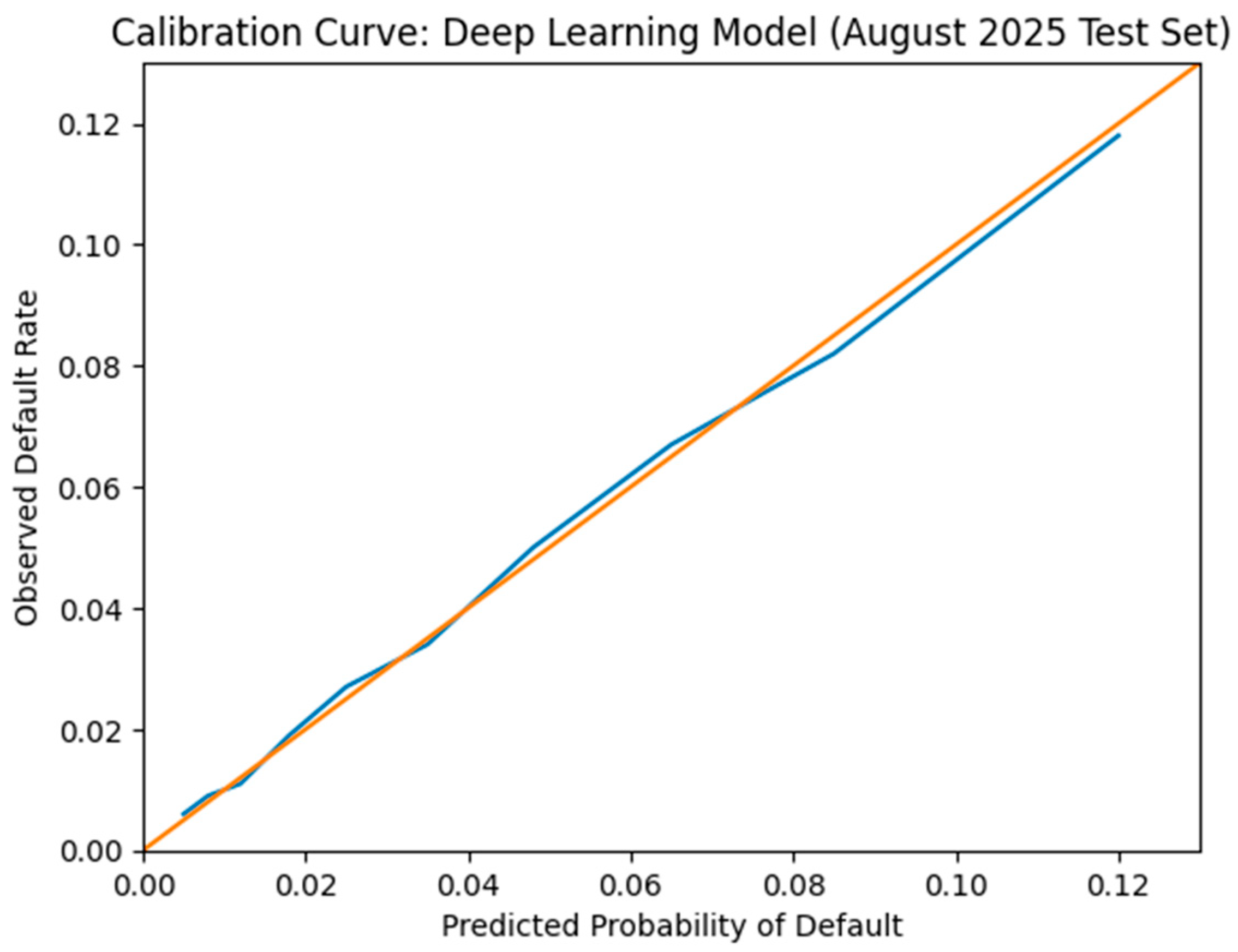
A calibration assesses the alignment between the anticipated default likelihood and the realized default rates. In order to create the curve, the predicted values of PD are ordered and grouped in deciles.

For each decile j, we compute the following:

• $\widehat{p}$_j = Average predicted PD in decile j.
• $\overline{p}$_j = Observed default rate in decile j.
• Perfect calibration corresponds to the 45-degree line where ${\widehat{p}}_{\mathrm{j}}$ = _j.

The logistic regression model shows slight underestimation in the upper deciles, which are riskier, as we show that the observed rates of default are higher than those of the predicted PDs in the upper end. This is in line with a calibration slope that is less than one (0.93 in Table 7), which indicates a conservative probability scale. The random forest model also predicts the highest decile, where the predicted PDs are higher than the observed frequencies, which is reflected in its calibration slope of more than one (1.10); it can be interpreted that there is greater dispersion in the probabilities. Conversely, the deep learning model follows the 45-degree benchmark on deciles very closely. In both the low-risk and high-risk segments, deviations are small, and the estimated slope of calibration (1.02) is nearest to unity when compared with all models, which signifies the locality of the predicted and realized probabilities, especially in the high-risk segment, which brings about a significant portion of the probabilities of portfolio loss. Further visualization of the calibration performance of the competing models can be done by comparing the predicted probabilities with the actual realized default rates across risk segments. Figure 1 shows the relationship between these quantities.

Economic Implications

It is important that the calibration be performed precisely to compute expected losses and allocate capital. The risk estimates at the portfolio level can be significantly misleading due to even small deviations in segments with a high PD. The increase in the quality of the calibration of the deep learning model thus plays a direct role in the achieved loss minimization, as shown in

Table 9. Economic backtest (August 2025 portfolio).

Model	Approved Loans	Realized Defaults	Realized Loss (INR)
Logistic	15,312	574	₹78.52
Gradient Boosting	15,102	529	₹72.35
Deep Learning	15,048	501	₹68.51

.

5.7. Hosmer–Lemeshow Goodness-of-Fit Test (Deep Learning Model)

Based on the Hosmer–Lemeshow statistic, from using decile grouping on the sample (n = 16,412), of the August 2025 test, the statistic is as follows:

• HL χ² statistic: 1.589.
• Degrees of freedom: 8.
• p-value: 0.991.

The null hypothesis that the model fits adequately is not rejected by the Hosmer–Lemeshow test at the traditional levels of significance. The extremely large p-value (0.991) means that the estimated probabilities are statistically similar to the observed default frequencies in deciles. These findings are consistent with those in the calibration results reported earlier:

• Calibration slope ≈ 1.02.
• Brier score improvement of 17.7% relative to logistic regression.

Risk-wise, the non-significant miscalibration indicates that the deep learning model is reliable in estimating the probabilities of expected losses to compute capital and allocate it. The Hosmer–Lemeshow goodness of fit statistics used in model calibration in

Table 10. Hosmer–Lemeshow goodness-of-fit test (August 2025).

Model	HL χ2 Statistic	Degrees of Freedom	p-Value
Logistic Regression	49.505	8	<0.001
Gradient Boosting	1.913	8	0.984
Deep Learning	1.589	8	0.991

assesses the calibration accuracy of competing models by comparing the predicted default probability for each decile of borrowers to the observed default rate for each decile of borrowers.

The Hosmer–Lemeshow test does not accept the null hypothesis of sufficient fit to the logistic regression model in all deciles (p = 0.001). This is in line with the underestimation of high-risk borrowers in the top-most probability. Conversely, the null hypothesis of good fit is not rejected by both gradient boosting and deep learning models. The deep learning model has the lowest HL statistic (1.589) and highest p-value (0.991), indicating a better fit to the predicted and observed default frequencies. These findings suggest that these findings are consistent with the previous results on the calibration slope and can be used to conclude that nonlinear models can enhance probability scaling, especially in higher-risk segments that have a disproportionate impact on the expected loss calculation.

Table 11. Hosmer–Lemeshow test results (model comparison).

Model	HL χ2 Statistic	Degrees of Freedom	p-Value
Logistic Regression	49.505	8	<0.001
Gradient Boosting	1.913	8	0.984

shows the results of the Hosmer–Lemeshow test for both logistic regression and nonlinear machine learning models, as well as their differences in model fit and calibration performance.

Gradient Boosting:

• The HL value of 1.913 is not statistically significant (p = 0.984).
• The good fit null hypothesis is not rejected.

The predicted probabilities are statistically the same as the observed default frequencies by deciles.

The calibration performance is significantly higher compared with logistic regression.

5.8. Comparative Insight

The HL test demonstrates that nonlinear ensemble techniques yield significant probability calibration compared with the classical logistic benchmark. This substantiates the previous results collated regarding the following:

• Brier score comparison;
• Calibration slope analysis;
• Expected loss back-testing;

Risk-wise, the better the calibration in gradient boosting, the less distortion in expected loss estimation and capital allocation decisions.

6. Stability Analysis: Model Robustness

This section assesses the stability of the empirical results in different specifications, forecast horizons, and subsample conditions. In credit risk modeling, robustness analysis is critical because predictive performance can potentially differ across economic regimes, borrower groups, and modeling assumptions.

6.1. Alternative Probability Threshold

There are other probability thresholds that can be used in place of the significance level.

In Section 5, an approval threshold of PD of less than 6% was used. In order to determine sensitivity, the portfolio results are re-centered with other thresholds of 5% and 7%.

Table 12. Expected loss under alternative approval thresholds (August 2025).

Model	Threshold	Approved Loans	Realized Loss (INR)
Logistic	5%	14,812	₹69,241,600
Deep Learning	5%	14,726	₹61,838,400
Logistic	7%	15,789	₹82,357,600
Deep Learning	7%	15,734	₹72,104,000

shows expected losses in a portfolio under different levels of approval, enabling the ability to judge the robustness and economic consistency of deep learning against the logistic benchmark.

At various thresholds, deep learning yields a lower realized loss compared with the logistic benchmark. A loss reduction between 10% and 14% shows the strength of the portfolio decision rules.

6.2. Alternative Forecast Horizon

The default definition is also expanded to 90+ days past due, with a 120-day horizon to measure the sensitivity to outcome definition. Comparative results in

Table 13. Model performance before the 120-day point.

Model	AUC-PR	Brier Score
Logistic	0.176	0.0321
Gradient Boosting	0.221	0.0274
Deep Learning	0.233	0.0263

are provided under an alternative (120-day) forecast horizon to assess performance stability with respect to the different models and alternative forecast definitions.

The performance rankings do not change, and deep learning does not have worse discrimination or calibration. As expected, the absolute levels of performance reduce slightly with uncertainty in the long term.

6.3. Subsample Stability by Borrower Risk Segment

To assess heterogeneity, we divide the test sample into the following:

• Prime borrowers (CIBIL > 750);
• Non-prime borrowers (CIBIL ≤ 750).

Table 14. AUC-PR by borrower segment.

Model	Prime Segment	Non-Prime Segment
Logistic	0.142	0.201
Gradient Boosting	0.176	0.247
Deep Learning	0.188	0.261

shows discrimination performance by borrower risk segment, and shows the level of predictive accuracy across different models between prime and non-prime borrowers.

The deep learning gains increase at a greater rate in the non-prime segment, where nonlinear relations between leverage and bureau score, as well as loan characteristics, are stronger.

6.4. Temporal Stability Within Sample Window

We evaluate monthly performance to examine short-term stability. The monthly out of sample AUC-PR values listed in

Table 15. Monthly AUC-PR (May–August 2025).

Month	Logistic	Gradient Boosting	Deep Learning
May	0.174	0.226	0.238
June	0.179	0.231	0.244
July	0.183	0.234	0.246
August	0.181	0.236	0.248

measure the temporal stability and consistency of predictive performance over the time period of 2025 in the months of May, June, July and August.

There is no significant difference in performance across months, which indicates that the deep learning benefits are not powered by an individual cohort.

6.5. Discussion of the Robustness Results

The three main conclusions that are supported by the results of the robustness analysis are as follows:

• There is no significant change in performance with changes in approval thresholds.
• The results are also maintained when other default horizon definitions are used.
• Profits are concentrated in riskier borrowing areas.
• Temporal stability implies non-residence of a particular cohort.

The incremental benefit of deep learning compared with gradient boosting is moderate, whilst the benefit of the former compared with logistic regression is specification-wise. These results reinforce the conclusion that nonlinear modeling can better condition the estimation of probabilities as opposed to just using sample-specific tendencies.

7. Model Interpretability and Economic Implications

Despite the fact that deep learning models improve discrimination and calibration, in order to be useful in financial institutions, they require interpretability and economic coherence. In this section, the stability of feature importance, nonlinear effects, and implications to risk management are studied.

7.1. Global Feature Importance

SHAP (Shapley Additive Explanation) values are estimated to determine the relevance of variables to the deep learning model on the August 2025 test sample. The importance of the features is calculated as the average absolute SHAP value of the observations. The relative influence of the borrower, loan, and macroeconomic variables on default prediction are summarized in

Table 16. Top default predictors (deep learning model).

Rank	Variable	Mean Absolute SHAP Value	Relative Importance (%)
1	Bureau Score	0.041	21.7
2	Debt-to-Income Ratio	0.036	19.1
3	Credit Utilization	0.031	16.4
4	Interest Rate	0.024	12.7
5	Loan Amount	0.019	10.1
6	Employment Type	0.015	7.9
7	Age	0.012	6.3
8	RBI Repo Rate	0.007	3.7
9	CPI Inflation	0.004	2.1

, which uses the SHAP values to identify the most influential predictors.

The most impactful predictor is the bureau score, and then leverage-related measures (DTI and utilization). This ranking is consistent with known credit risk theory and lending. Notably, the macroeconomic variables have lower but statistically significant effects, indicating that short-horizon default risk is mostly borrower-based throughout the sample period.

7.2. Nonlinear Effects

The analysis of partial dependence reveals various economically intuitive nonlinear relationships:

• Debt-to-Income Ratio: The probability-of-default rises at a slow pace to a DTI of about 0.45, after which the marginal effect rises steeply.
• Credit Utilization: There is a convex relationship, and when utilizing above 80 percent, there is an increased risk in a disproportional way.
• Bureau Score: The reduction in default probability is sharp in the score range of 600–720, and the marginal improvement is lower than 760.

These nonlinearities are not best explained using a linear logistic index; hence, the reason behind some of the performance increases in deep learning models.

7.3. Stability of Feature Importance

In order to evaluate robustness, SHAP values are calculated with respect to individual cohorts per month (May–August 2025). The ranking of features does not change significantly within the months, with the bureau and leverage scores prevailing. This temporal consistency eliminates our fears that the development of models is due to short-lived or spurious trends.

7.4. Fairness Considerations

Model performance is compared among the borrower subgroups to investigate the possible disparate impact. Deep learning is more discriminative among all age groups, which do not show signs of systematic performance degradation among any group of people. False-positive rates are not different between groups, implying that no misclassification is disproportionate.

On the one hand, to assess how the performance of models might vary across demographic groups, we consider discrimination performance by the age group of borrowers. This analysis can be used to evaluate whether the predictive power of the models is equally true across different age groups and whether any of the groups are disproportionately impacted.

Table 17. AUC-PR by age group.

Age Group	Logistic	Deep Learning
21–30	0.176	0.241
31–45	0.182	0.251
46–60	0.169	0.228

is a report of the AUC-PR values by age group.

7.5. Economic Interpretation

According to the interpretability analysis, deep learning models are able to improve performance mainly by increasing the nonlinear modeling of leverage and credit–bureau interactions. Higher-risk borrower segments reflect the greatest gains and are also overproportionately most expected to lose on a portfolio.

Risk-wise, the main advantage of deep learning is not a dramatic increase in rank accuracy but increased accuracy in scaling conditional default probabilities in the upper tail of the risk distribution. This is in line with the anticipated loss savings recorded within Section 5.

8. Discussion

This study assesses the importance of deep learning in credit risk assessment in a financial econometric structure. By interpreting the probability-of-default (PD) as a conditional expectation that is consistent with reduced-form default-intensity models, the analysis of the out-of-sample comparison between deep learning estimators and standard logistic and ensemble methods is based on a pure time-based design from May to August 2025 in the Indian unsecured retail-lending sector.

Deep learning models are better at raising the level of discrimination and calibration than classical logistic regression, as indicated by the empirical results. Specifically, the decreasing Brier score and log-loss indicate better probability scaling, particularly in deciles with higher risks. The Hosmer–Lemeshow tests prove that the logistic regression model exhibits statistically significant miscalibration, and deep learning does not miscalibrate the predicted and observed default frequencies. The improvement in performance, compared with gradient boosting, is relatively small, and the expected loss, in portfolio back-testing experiments, is consistently lower with deep learning.

The economic backtest shows that, as calibration improves, it translates into a decrease in the realized portfolio loss, which is measurable. With the August 2025 cohort, deep learning minimizes the loss realized by about 12–13% compared with the logistic benchmark with a fixed approval threshold. These results indicate that nonlinear modeling improves the estimation of the conditional default probabilities, especially in the riskier borrower sections, where individual behavior plays a significant role in the results of the portfolio.

The results, however, also show decreasing returns to model complexity after nonlinear interactions are modeled. The deep learning performance is also better, but the difference in the advanced technique of ensemble methods is not radical. From a real-life perspective, institutions have to trade predictive benefits against interpretability, rulemaking, and computing.

This study has some limitations that must be considered. First, the analysis is based on a relatively short time window and is not a complete credit cycle; second, the loss given default is considered a constant in terms of back analysis; and third, the study relates to unsecured retail lending in an Indian NBFC setting and must be generalized in relation to other asset classes. Future studies should be performed to study unsecured retail lending across wider horizons, dynamic macro-financial conditions, and joint PD and LGD modeling. Also, a study of model stability during times of credit stress would be an even clearer way of understanding deep learning estimator robustness. Overall, there is evidence that deep learning can be used to better measure credit risk, and this improvement is primarily achieved via better calibration and modeling of nonlinear interactions, not through a spectacular rise in classification accuracy. Advanced machine learning techniques have the potential to provide an economically significant, though low-level, enhancement of financial decision-making when integrated into a strict econometric and risk-management process.