1. Introduction
The goal of this study is to assess the merits of incorporating a lending-value criterion into the design of portfolios held by institutions with a long-term investment horizon, such as pension funds, university endowments, most insurance companies, and many family offices. These institutions typically maintain sizable positions in alternative assets. Because such assets are illiquid, being forced to dispose of them under stressful market conditions can result in substantial losses. This occurred, for example, in the aftermath of the subprime crisis (2007–2008). A similar situation arose in early 2022, when a decline of more than 20% in the value of U.S. stocks altered portfolio asset mixes and forced some managers to rebalance their positions (e.g., selling alternative assets to comply with maximum exposure limits dictated by covenants). One way to avoid these situations—that is, the necessity of selling illiquid assets under unfavorable market conditions—is to rely on credit lines to navigate periods of financial stress. This, of course, presumes the ability of the portfolio manager to use the portfolio as collateral, which, in turn, raises the question of whether such portfolios should be constructed with a minimum lending-value criterion in addition to the usual risk-and-return objectives.
This study explores the merits of incorporating this feature into the portfolio construction process. Although several studies have examined the addition of alternative criteria to the conventional portfolio optimization framework (a topic reviewed in the next section), to the best of our knowledge, the lending-value potential—or, equivalently, the borrowing capacity—of portfolios in the context of long-term investment vehicles has not been investigated. (Notice that these vehicles typically rely on buy-and-hold strategies rather than active trading strategies.)
The remainder of this paper is organized as follows. The next section reviews the relevant literature. The following section formulates the problem in more formal terms, after which we describe the data and its sources. We then present the empirical analyses and discuss the corresponding results. The paper concludes with a summary of the main findings and their implications.
2. Review of Previous Work
During the second half of the twentieth century, treatment of the portfolio selection problem—namely, how to allocate a given budget among several asset classes—was dominated by Markowitz’s framework and its many permutations (
Markowitz, 1952). By “Markowitz’s framework,” we refer to the idea that asset allocation (i.e., portfolio weights) should be determined by solving an optimization problem aimed at maximizing the expected return subject to a risk constraint expressed in terms of the standard deviation of returns. Since the late 1990s and early 2000s, however, two new tendencies began to emerge in the financial engineering landscape, both driven more by practitioners than by academics. The first was a gradual shift from the standard deviation to the Conditional Value-at-Risk (CVaR) as the preferred risk metric (
Rockafellar & Uryasev, 2000). This shift reflected the recognition that the CVaR directly measures potential losses, what investors truly care about, whereas the standard deviation only measures volatility and cannot distinguish between favorable and unfavorable outcomes.
Note: the Value-at-Risk, or VaR—a risk metric introduced in the late 1990s—was initially viewed as a promising alternative to the standard deviation of returns (
J.P. Morgan, 1994). However, the VaR violates a mathematical condition known as subadditivity, which is problematic in the context of portfolio construction because it can, in some cases, penalize diversification. This limitation explains why the Conditional Value-at-Risk (CVaR), developed shortly after the VaR and free of this drawback, was quickly adopted by financial practitioners once it was introduced (
Artzner et al., 1999).
A second tendency, more relevant in the context of this study, was the incorporation of additional criteria, beyond risk, into the optimization problem. For example,
Ballestero et al. (
2012),
Utz and Wimmer (
2014), and
Utz et al. (
2015) introduced environmentally responsible restrictions based on sustainability scores.
Ceren and Koksalan (
2014),
Qi et al. (
2017),
Vieira and Filomena (
2020), and
Barro et al. (
2024) investigated the inclusion of liquidity constraints—a strand of research particularly relevant to the present study, as liquidity is closely related to the concept of advance rates explored herein.
Arcuri et al. (
2023) incorporated the investor’s risk aversion profile, while
Hilario-Caballero et al. (
2020) examined the implications of imposing low-carbon emissions restrictions.
Katsikis et al. (
2021) incorporated transaction costs into the Markowitz framework, which they modified slightly by adding a penalty function. In a similar spirit,
Mamanis (
2021) modified the Markowitz model by incorporating three objectives, with the aim of improving the out-of-sample performance by considering the shape of the return distribution.
Grizickas Sapkute et al. (
2022) and
Sheng and Shen (
2020) addressed the effects of regulatory constraints on the portfolio selection problem; these studies, along with the liquidity-focused contributions cited above, constitute the strands of literature most closely adjacent to the present work. Conclusions from regulatory studies, however, must be interpreted with caution, as they often apply only to very specific markets.
Hirschberger et al. (
2013) and
Steuer et al. (
2007) focused on more theoretical aspects of what they termed the multiple-objective portfolio selection problem—for example, deriving explicit formulas to determine the nondominated surface when risk is measured by the standard deviation of returns. Some of the most theoretical contributions (e.g.,
Steuer et al., 2007), notwithstanding their merits, are unlikely to be of practical use to portfolio managers and practitioners. In contrast, many empirically based studies offer useful insights. For example,
Ballestero et al. (
2012) showed that “green” investors, compared to more conventional investors, must be willing to tolerate greater risk in their portfolios. This result is not surprising, given that adding a constraint to an optimization problem reduces the size of the feasible set. This finding has been confirmed by
Lara Moreno and Hernandez Castellanos (
2024), who incorporated an ESG-index constraint into the optimization problem and concluded that their formulation could help investors assess what they call the “deterioration level”—that is, the effect on return of adding the ESG condition to the traditional Markowitz formulation. More recently,
Utz and Steuer (
2025) suggested, perhaps more optimistically, that incorporating climate risk metrics into the portfolio selection problem would affect returns only marginally. Along the same lines,
Garcia et al. (
2019) explored how to address the portfolio selection problem through a fuzzy-logic approach combined with ESG-score constraints. Regrettably, they did not compare their results with those obtained without the ESG constraint.
Nevertheless, the interpretation of results from incorporating ESG-based constraints—or, more generally, sustainability considerations—into portfolio selection problems must be approached with caution. One reason is that ESG ratings, which often serve as the basis for such constraints, are plagued by ambiguities and a lack of consistency (see, e.g.,
Charlin et al., 2024;
Billio et al., 2021). Moreover, when these constraints rely on unaudited data, the risk of distortion due to greenwashing is significant (
Santos et al., 2024).
A salient feature of most empirical studies is their reliance on historical returns covering relatively short time periods. For example:
Ballestero et al. (
2012), 2001–2006;
Ceren and Koksalan (
2014), 2005–2010;
Barro et al. (
2024), 2016–2023;
Tuncer Sakar and Koksalan (
2013), 2003–2009;
Lara Moreno and Hernandez Castellanos (
2024), 2021–2023;
Garcia et al. (
2019), 2014–2017. Studies that examined longer horizons often focused on local markets with limited global relevance. For instance,
Vieira and Filomena (
2020) relied on 2007–2016 data from the Brazilian stock market, while
Dächert et al. (
2022) analyzed the German insurance sector using artificial data (i.e., slightly modified real returns, according to the authors).
At present, no study has relied on returns data spanning both the subprime crisis and the COVID-19 crisis, two highly relevant periods of financial stress. Another characteristic of most previous studies—which should not be taken as a criticism—is their focus on the shape and features of the efficient frontier (or nondominated frontier) rather than on changes in portfolio composition (i.e., asset weights) resulting from the incorporation of additional constraints.
Moreover, the lending value of a portfolio, the focus of this study, has not been addressed in prior research. The lending value of an asset is expressed through a parameter known as the advance rate (AR), which represents the maximum loan amount, as a percentage of the asset’s market value, that a lender is willing to offer. Highly liquid assets, such as Treasuries, typically enjoy high ARs, while less liquid assets—such as private equity or venture capital investments—receive much lower ARs. Clearly, liquidity and ARs are closely correlated: liquid assets generally exhibit lower volatility and more stable prices, which justify higher ARs, whereas illiquid assets are more volatile and, in many cases, lack an active secondary market, resulting in conservative ARs to account for price uncertainty. In this sense, the present study extends the liquidity-constraint literature by introducing a criterion—the lending value of the portfolio—that captures liquidity indirectly through its regulatory and institutional manifestation in the form of ARs, as established by standard industry and regulatory practice (
FINRA & U.S. SEC, Office of Investor Education and Advocacy, 2015;
OCC, 2017).
Although several studies have examined the use of liquidity constraints in portfolio optimization, they provide limited insight into the lending-value potential of long-term investment vehicles. Such studies focus on portfolios composed of stocks and investment-grade bonds, whose liquidity can be readily assessed via bid-ask spreads or metrics such as
Amihud (
2002),
Qi et al. (
2017), and
Lo et al. (
2003). Long-term portfolios, in contrast, often include private equity funds, direct lending funds, art, and emerging market assets—assets for which secondary markets are thin and traditional liquidity metrics are not applicable. Furthermore, many liquidity studies emphasize constraints based on trading volumes, which are largely irrelevant for long-term funds that typically follow buy-and-hold strategies. Indeed, most long-term funds conduct rebalancing exercises infrequently, often only once or twice per year.
A recent study by
Arcuri et al. (
2023), which examines portfolios of certain Italian institutions known as Foundations of Banking Origin (FBOs), is based on portfolios whose composition closely resembles that of American endowments. These portfolios include not only stocks and bonds but also real estate, venture capital, and art investments. The focus of their study, however, was not on the lending value of these portfolios but on incorporating the investor’s risk profile as an additional criterion. Finally,
Arcuri et al. (
2023), along with
Barro et al. (
2024), provide a detailed and up-to-date review of the literature on portfolio optimization problems with multiple objectives.
Building on this background, the present study seeks to address this gap; specifically, it extends the adjacent literature on liquidity constraints, collateral-based financing, and regulatory frameworks by introducing lending value—operationalized through ARs—as an explicit constraint in the optimization framework. The analysis relies on historical data covering both the subprime crisis and the COVID-19 crisis and includes asset classes that reflect the actual holdings of these portfolios, not just stocks and bonds. Furthermore, the optimization framework is based on realistic target returns, a topic discussed in greater detail in
Section 5.
3. Problem Statement
The problem at hand can be formalized as follows. It is assumed that there are asset classes (each described by a suitable index), (monthly) periods, and a target return . Let be the return of asset class in period . Finally, let represent the vector of assets weights and be the vector of expected asset returns.
The conventional optimization problem can be cast as follows:
subject to
and
where
refers to the CVaR estimated based on the worst
loss scenarios. Notice that the components of the vector of expected asset returns,
can be estimated as follows:
To this formulation, it is necessary to add the lending-value constraint, which can be expressed in terms of the portfolio weighted-average advance rate, or
PAR. That is
where
λp denotes the AR associated with asset class
p, and
L is the minimum (desired) lending-value target.
The non-negativity constraint on portfolio weights reflects the fact that long-term institutional investors—such as university endowments, family offices, and pension funds—do not typically engage in short selling (
Molk & Partnoy, 2019;
Nagel, 2005). Short selling is more commonly employed as an investment strategy in the context of hedge funds and other speculative vehicles, which fall outside the scope of this study.
Note that the optimization problem can be formulated in two equivalent ways: either by maximizing the return subject to a risk constraint or by minimizing the risk subject to a return constraint. The former formulation is more common in the academic literature, whereas the latter aligns more closely with how practitioners—specifically, portfolio managers—approach the problem. Notably, long-term investment funds typically have precise target returns, specified either by their covenants or by their boards each year. Therefore, a formulation based on a specific target return is more appropriate from a practical standpoint.
Also, recall that
Rockafellar and Uryasev (
2000) demonstrated that the CVaR-based optimization problem can be efficiently formulated as a linear programming problem, which is quite convenient from a computational perspective. Importantly, adding a lending-value constraint, being linear, does not compromise this advantage. A thorough discussion of this implementation is addressed in
Gutierrez et al. (
2019). Note that linear optimization problems can be solved easily using freely available, open-source software packages. Alternatively, given the fact that the CVaR is convex and all of the constraints are linear, the optimization problem can also be tackled directly, again, using off-the-shelf, open-source software packages. In both cases, the CVaR needs to be estimated discretely, that is, based on a series of return observations, rather than parametrically using a model fitted to the relevant data. The advantage of this approach is that it better captures the effect of the outliers.
Section 5 discusses the CVaR calculation in more detail.
4. The Data
Seven indices, each representing a relevant segment (asset class) of the global economy, were selected. Based on the values of these indices, monthly returns were calculated for the period January 2004–December 2023. The data were obtained from Bloomberg, Yahoo Finance, and the St. Louis Federal Reserve websites.
Table 1 provides a description of the indices along with some of their key attributes. The asset classes considered comprise a mix of conventional and alternative assets. The definition of alternative assets is somewhat fluid: real estate and private equity are consistently classified as alternatives, while high-yield bonds and emerging market equities occupy a gray area. In any case, the selected asset classes reflect the typical holdings of an American university endowment (
Hatton, 2024) and are similar to the asset mix employed by
Arcuri et al. (
2023).
It is important to note that the Sharpe ratios reported in this table play no role in the modeling framework described in the previous section. They are included solely to provide a broad indication of the relative risk-adjusted performance of each asset class. Given the well-known ambiguities surrounding the choice of an appropriate risk-free rate, we set this value to zero for the purpose of this calculation. That said, the figures are broadly consistent with what one would expect. For instance, global equities (0.17213) show superior risk-adjusted returns relative to emerging market equities (0.12608), and investment-grade bonds (0.12217) have outperformed real estate (0.07119) on the same basis. None of these comparisons should come as a surprise to practitioners familiar with the long-run behavior of these asset classes. We stress, however, that these figures represent averages computed over the full sample period (2004–2023) and are not intended to capture any short-term dynamics or cyclical patterns. They should be interpreted as long-run stylized facts.
The 2004–2023 period offers two advantages: it is sufficiently long to ensure an acceptable level of representativeness and it encompasses two periods of significant market stress—the subprime crisis (2007–2008) and the COVID-19 crisis (2020–2022).
Table 1 also reports the ARs by asset class. The AR represents the proportion of an asset’s market value that a lending institution is willing to extend as credit against a specified collateral position (
FINRA & U.S. SEC, Office of Investor Education and Advocacy, 2015;
OCC, 2017). A defining characteristic of ARs is their stability: unlike market prices or credit spreads, these rates do not adjust materially during periods of financial stress. This stability is not accidental: ARs are calibrated using long-run historical data precisely to incorporate the potential deterioration in collateral values during episodes of market dislocation, including systemic crises. The possibility of sharp asset price declines is thus already embedded in these rates, rendering real-time adjustments unnecessary. This feature is clearly reflected in the variation observed across asset classes: U.S. Treasuries command a high AR, given their low volatility, deep liquidity, and preeminent status as safe-haven assets. By contrast, assets such as emerging market equities are assigned substantially lower ARs, reflecting their high volatility, thinner liquidity, and heightened sensitivity to global geopolitical and macroeconomic shocks. It is important to note that the ARs are exogenous to the problem under analysis: they enter the model as inputs specified in common industry standards; they are not determined within the framework of the analysis.
Finally, the CVaR was calculated with a 90% confidence, a common choice among practitioners (e.g.,
Ceren & Koksalan, 2014).
5. Results and Analyses
The dataset was segmented into 16 overlapping five-year windows—[2004–2008], [2005–2009], …, [2019–2023]—to facilitate the identification of distinct market regimes. This methodological choice allows for a more nuanced analysis than a single-window evaluation of the full dataset, as it enables the investigation of effects across different market regimes. (Recall that return time series are non-stationary, and shifts in market regimes are not anomalies but intrinsic features of such series.) Moreover, the use of multiple five-year windows has been successfully employed by other researchers in previous studies (e.g.,
Peña et al., 2024;
Pagnoncelli et al., 2017).
The first set of analyses, based on the framework described above, involved determining the efficient frontier for each time window. Two scenarios were considered: (i) portfolio optimization without a lending-value constraint, corresponding to the standard formulation described in (1)–(5); and (ii) portfolio optimization incorporating several variations of the lending-value constraint (different L values), as described in (6). Ten target-return values were selected to construct each efficient frontier curve. These values differed across time windows, reflecting the maximum and minimum returns delivered by the indices in each respective window. The purpose of these analyses was to assess the potential impact of the lending-value constraint on the overall behavior of the efficient frontier.
Computation of the CVaR—a key ingredient in the optimization process—was carried out with a 90% confidence level using a discrete approach. Specifically, each five-year rolling window contained 60 monthly observations (past returns) for each asset, yielding 60 return vectors of size seven, corresponding to the seven asset classes under consideration. For a given asset allocation vector ω, the portfolio return associated with each of the 60 return vectors was calculated as the dot product of ω and the respective size-seven return vector. These 60 portfolio returns were then ranked in ascending order, and the CVaR was computed as the average of the six worst returns—consistent with a 10% cutoff applied to the 90% confidence level.
As expected, very high values of L (L > 0.75) frequently resulted in optimization problems with no feasible solution, while very low values of L (L < 0.40) produced non-binding constraints. Perhaps more surprising, however, was the extent to which the lending-value constraint was irrelevant (not binding), occurring in 10 of the 16 time windows considered. The constraint was only significant for time windows 6 through 9 ([2009–2016]) and 11 and 12 ([2014–2019]). This outcome was largely due to a non-negligible fraction of the portfolio being allocated to assets with low ARs (e.g., high-yield bonds) in the absence of the lending-value constraint, thus introducing the constraint of limited exposure to these assets.
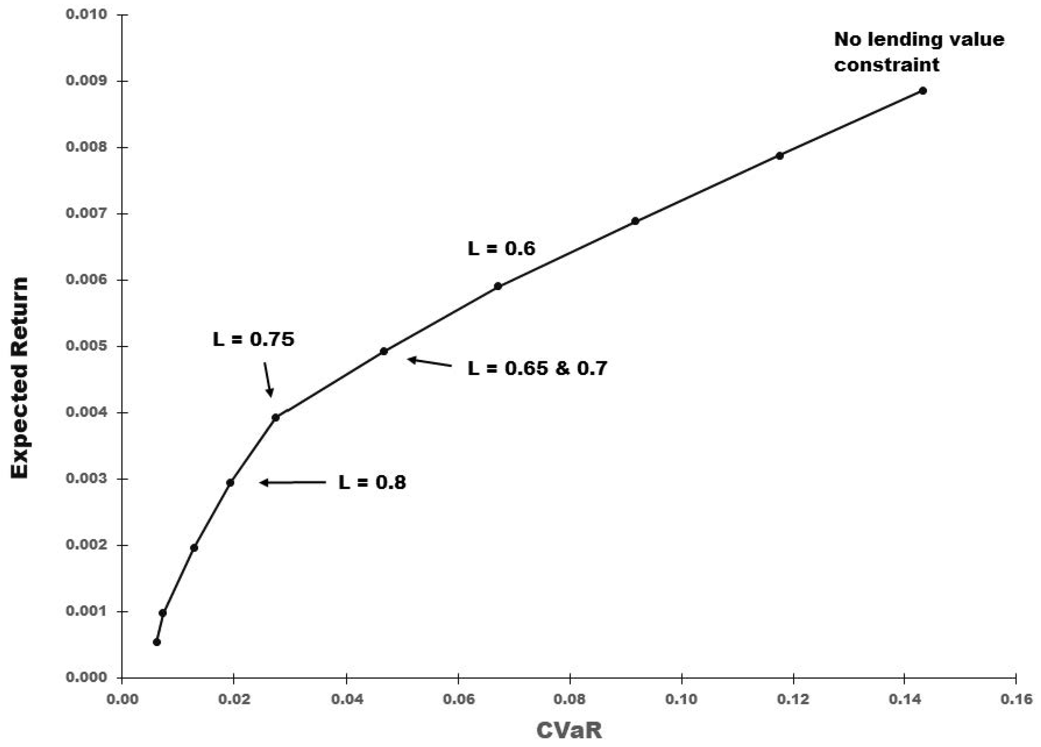
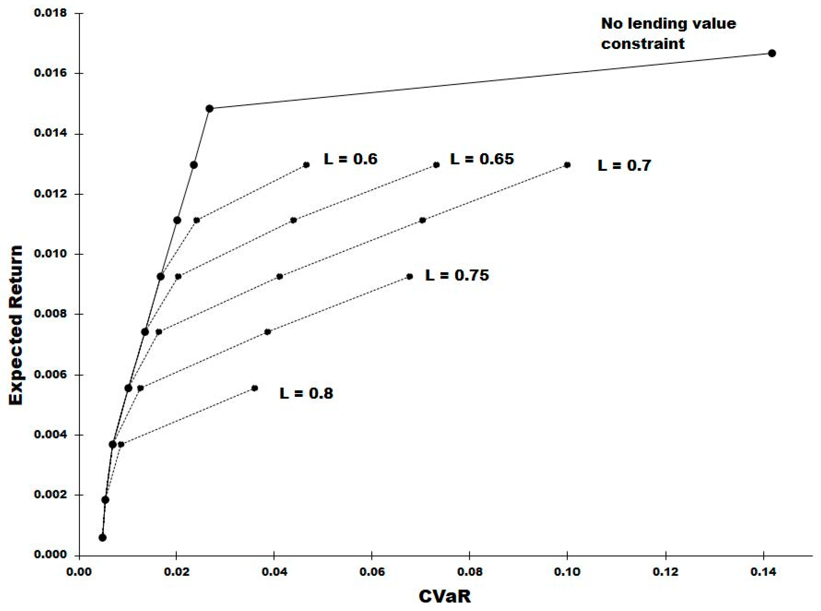
Figure 1 and
Figure 2 illustrate two families of efficient frontiers. In the first case (
Figure 1, time window 1, [2004–2008]), the curves overlap entirely. In the second case (
Figure 2, time window 6, [2009–2013]), the curves are clearly separated. Consistent with previous studies,
Figure 2 shows the efficient frontiers shifting markedly to the right as the lending-value constraints become tighter (e.g.,
Ceren & Koksalan, 2014;
Steuer et al., 2007).
The second, and far more important, analysis in this study aimed to explore the relevance of the lending-value constraint when the optimization problem is based on realistic target returns and reasonable lending-value limits—that is, parameters representative of the challenges faced by managers of long-term investment vehicles. (Ignoring these elements would be purely a theoretical exercise with no practical relevance.) To achieve this, it was necessary to estimate the range of target returns and L values (lending-value constraints) that are relevant in a realistic setting.
Target (nominal) returns for endowments are set by estimating next-year inflation and adding a spread that typically ranges between 4% and 5% (see
Table 2). The values presented in this table are based on this criterion and are consistent with empirical evidence. For example, the National Association of College and University Business Officers (NACUBO) reported that 15-year annualized returns for university endowments averaged 7.3% (
NACUBO & TIAA, 2021). Similarly, Pensions & Investments reported that, over the last ten years, the Columbia University and University of California endowments achieved average returns of 7.4% and 8.1%, respectively (
Pensions and Investments, 2024).
In theory, the lending value (i.e., the AR) of a portfolio could be very high, approaching 80% or 90%. In practice, however, values above 65–70%, even if the portfolio could theoretically support such ARs, would result in a debt ratio incompatible with the desirable typical risk profile of most endowments, even when considering short-term debt (the type addressed in this study). Additionally, such leverage could negatively affect the credit rating of the institutions holding these portfolios. Conversely, a portfolio with an AR around 50% is generally well-positioned to cover temporary imbalances arising from the need to rebalance asset weights or address other contingencies via credit lines. Based on the previous analyses, constraints dictated by values of L < 50% are largely irrelevant, suggesting that the practical importance of the lending-value constraint may be less than initially assumed.
Taking a conservative approach, two target-return cases (based on the values shown in
Table 2) were investigated for each of the 16 time windows. For each case, three scenarios were considered: (i) no lending-value constraint; (ii) a lending-value constraint defined by
L = 55%; and (iii) a lending-value constraint defined by
L = 60%, noting that these
L values are likely higher than what a long-term portfolio would realistically require. This exercise assumes that, at the end of each five-year period, the portfolio manager has accurately predicted next-year inflation and set the target return accordingly. The key question is whether the lending-value constraint is relevant under these target-return assumptions.
The results of these analyses are presented in
Table 3 and
Table 4, based on the target returns indicated in
Table 2 (Cases 1 and 2). The top panel of
Table 3, corresponding to the scenario without a lending-value constraint, is particularly revealing: in all time windows, the portfolio’s lending value (AR, second rightmost column) exceeds 50%, sufficient to secure a credit line capable of navigating stressful market conditions. This is a significant finding, as the 16 time windows encompass diverse market regimes, including highly stressful periods such as the subprime crisis (time windows 1–4) and the COVID-19 crisis (time windows 13–16).
Additionally, all portfolios exhibit a reasonable level of diversification according to the Modified Herfindahl–Hirschman Index (MHHI) (
Charlin & Cifuentes, 2021). Recall that values close to zero indicate poorly diversified portfolios, whereas values near 1 reflect high diversification. The exception is time window 15, which shows a portfolio concentrated in global stocks; however, this characterization may overstate the concentration, given that the index itself is highly diversified. Such sectoral concentrations are not uncommon and frequently occur when using Markowitz’s framework without constraints (see, for example, Figure 5 in
Barro et al., 2024).
The changes in asset weights (ω’s) across time windows are consistent with expectations. For instance, large weights were assigned to global stocks in recent years due to the strong performance of the S&P 500, and significant positions in Treasuries were observed following the subprime crisis (time windows 6 and 7). The minimal allocation to real estate and absence of private equity across all time windows reflect the combined effect of low Sharpe ratios and unfavorable CVaRs (see
Table 1) associated with these assets. This outcome is similar to the findings of
Barro et al. (
2024) and
Arcuri et al. (
2023), who, despite analyzing different constraints (liquidity and risk aversion), also observed minimal exposure to these asset classes.
The middle and bottom panels of
Table 3 present the results of incorporating the lending-value constraint (
L = 0.55 and 0.60), reporting only time windows in which the ω’s changed relative to the reference scenario (no lending value constraint). In both cases, adding the constraint results in a small but noticeable increase in risk (measured via CVaR). However, the lending-value constraint significantly enhances portfolio diversification (MHHI). For example, in time window 8, the MHHI increases from 0.34 to 0.72 when a lending value (
L = 0.60) constraint is added. This finding, somewhat unexpected, contrasts with
Barro et al. (
2024), who concluded that tighter liquidity targets (not identical to ARs, though correlated) reduced diversification. Conversely, these results support
Grauer and Shen (
2000), who found that additional constraints tend to yield more diversified portfolios.
Moreover, the lending-value constraint can materially alter asset allocation weights. For instance, in time window 12, introducing the lending constraint (
L = 0.60) changes the allocation to investment-grade and high-yield bonds from 0.16 and 0.79, respectively, to 0.31 and 0.48. While caveats apply, similar qualitative effects can be observed in the graphs presented by
Barro et al. (
2024). In short, adding the lending value constraint, in general, tends to lower the exposure to assets with low lending value (relatively speaking), such as HY bonds, and increase the exposure to assets such as IG bonds, that are associated with higher ARs.
These observations are also applicable to the results presented in
Table 4. It should be noted, however, that the optimization failed in time window 15 due to the high target return (9.1% annually), which was incompatible with the returns achieved by the assets available in that period. A minor difference compared to
Table 3 is that
Table 4 exhibits a more pronounced increase in risk when the lending-value constraint is applied. For example, the CVaR in time window 12 rises from 0.0260 (no constraint) to 0.0315 when the
L = 0.60 constraint is imposed.
To test the robustness of the results, two additional sets of analyses were conducted. These tests were analogous to the ones previously described, with minor modifications. First, the analyses were repeated using seven-year windows instead of five-year windows. Second, the asset classes considered were varied: in one case, investment-grade (IG) bonds were replaced with a gold index, and in the other, Treasuries were substituted with the gold index. These results (not reported herein) confirmed the previous findings. In essence, adding the lending-value constraint had either no effect or only a marginal effect, and all observations made in the earlier analyses remain valid.
In summary, it can be concluded that incorporating a lending-value constraint into the standard portfolio optimization problem is generally unnecessary. Portfolios constructed without this constraint already exhibit adequate lending value, as reflected in their average ARs.
6. Conclusions
The idea of including lending-value constraints in the construction of long-term portfolios appears, in principle, prudent. However, the empirical evidence presented in this study casts significant doubt on the potential merits of this practice. In short, the lending-value constraint is largely irrelevant, as the asset weights selected using the standard optimization framework already produce portfolios with adequate lending value. The robustness of this conclusion is supported by the fact that the study covers a variety of market regimes over a twenty-year period, including both the subprime and COVID-19 crises—no previous studies have relied on data spanning these two periods.
Nevertheless, it is important to recognize that future crises could differ substantially from those examined herein. For example, a future crisis might be driven by factors distinct from the subprime or COVID-19 crises, such as a trade war or a large-scale sell-off of Treasuries by a major central bank. Such events could also occur in a more inflationary environment, unlike the relatively benign inflation levels observed during the two crises studied. Under these conditions, lending-value constraints might assume a more significant role.
While it may be tempting to draw absolute conclusions, these results should be interpreted with caution. They are based on the assumption that the portfolios analyzed are long-term portfolios that are not actively traded. Extrapolating these findings to actively managed portfolios, hedge funds, or, more generally, portfolios with a short-term investment horizon or employing aggressive or speculative strategies would be inappropriate. Such vehicles typically rely on derivatives, carry trades, short selling, and other instruments that were not included in our formulation. In brief, these types of portfolios fall outside the scope of the present analyses.
Finally, from a practical standpoint, two recommendations emerge from this study. First, from a portfolio management perspective, given that the lending-value constraint is generally not binding, a sensible approach is to perform portfolio optimization without incorporating this constraint. If an ex-post review indicates that the resulting asset weights fail to meet a minimum lending-value requirement, only then should a second optimization, including the lending-value constraint (minimum AR limit), be conducted.
Second, from a governance perspective, it is important that the bylaws of long-term investment vehicles explicitly permit borrowing. Without this flexibility, a fund—even if its portfolio provides an adequate AR—could be forced to sell assets under adverse market conditions.
Two topics warrant further research. One is determining the optimal leverage level (short- or long-term) for such portfolios under varying market regimes. Another is formally assessing the impact of additional constraints on portfolio diversification, whether positive or negative.