How Do IFRS S2 Climate Risks Affect IAS 36 Impairments? A Constructive Accounting Framework Calibrated to European Steel

Abstract

A major connectivity gap arises from the misalignment between the forward-looking climate disclosures required by IFRS S2 and the historically rooted asset valuations mandated by IAS 36. This misalignment can cause the overvaluation of carbon-intensive assets and disrupt capital allocation decisions. This research specifically examines transition risks, such as carbon pricing, regulatory shocks, and technological disruption, and quantifies the financial externality using a combination of deterministic impairment testing and stochastic climate scenarios. We create a constructive framework and develop a model of a Synthetic Representative Firm, calibrated to major integrated steel producers in Europe. To generate nonlinear Green Swan shocks for Value-in-Use, the process combines Monte Carlo simulation with the Merton Jump-Diffusion model. This comparison shows the difference between the steady Management View and the volatile Market View. Empirical results reveal a material Sustainability Discount, representing a substantial erosion in the recoverable amount under IFRS S2 transition risk scenarios compared to the IAS 36 Deterministic Baseline. Simulations show a strong probability of asset stranding due to restricted cost pass-through, indicating that older assets may face elevated impairment risks under disorderly transition scenarios. Traditional deterministic models may not fully capture aspects of Double Materiality, potentially leaving balance sheets less responsive to transition risks. Integrating digitalization and the Circular Carbon Economy (CCE) framework presents a strategic method for averting value destruction. Therefore, this research supports the integration of stochastic transition risk modeling into impairment testing to achieve faithful financial representation.

1. Introduction

The modern financial reporting landscape exhibits a notable connectivity gap (IFRS Foundation, 2023). On the one hand, under IFRS S2 Climate-related Disclosures, firms are becoming more transparent about the existential risks associated with a transition to a low-carbon economy, including issues such as carbon pricing and technological obsolescence. Conversely, financial statements prepared in accordance with IAS 36 Impairment of Assets reflect a business-as-usual valuation, assuming assets can continue indefinitely. This disconnect aligns with Brunsson’s (1989) concept of organizational hypocrisy, where sustainability reports and financial measurements are structurally separate. This gap reveals a failure to implement the Double Materiality principle, in which the financial effects of environmental risks are not integrated into corporate metrics (Nielsen, 2023). As the global economy nears critical tipping points outlined in the World Energy Outlook 2025 (IEA, 2025), this divide becomes increasingly unsustainable. The emergence of Green Swan events, rare but impactful climate shocks with systemic financial effects (Bolton et al., 2020), threatens to turn billions in book value into stranded assets (Caldecott, 2017), exposing a looming crisis that current accounting models cannot adequately address.

This study focuses specifically on transition climate risks (carbon pricing, regulatory shocks, and technological disruption) as defined under IFRS S2, as these risks are directly quantifiable within valuation models through their impact on cost structures and cash flows. While IFRS S2 encompasses both transition and physical risks, the latter (e.g., extreme weather events, asset damage, and operational disruptions) involve distinct modeling challenges and are not explicitly incorporated in the present framework. The rationale for this scope delimitation is discussed in the last section.

However, while these transition risks are theoretically quantifiable, the core of this problem lies not in the absence of data, but in the methodological limitations of the valuation models currently entrenched in accounting practice. Traditional impairment testing under IAS 36 predominantly relies on Deterministic Baseline (GBM Specification)-based Discounted Cash Flow (DCF) models or Value in Use (VIU) calculations that assume continuous, linear economic progression. These models, grounded in the Geometric Brownian Motion (GBM) framework of Black and Scholes (1973), assume normally distributed returns, which leads to an understatement of extreme outcomes typically captured in the tail risks of the distribution. Yet, recent empirical evidence from carbon markets contradicts this assumption. Gronwald and Ketterer (2012) and recent analyses of the EU Emissions Trading System (EU ETS) demonstrate that carbon prices exhibit heavy tails and discontinuous jumps driven by sudden regulatory interventions (Benz & Trück, 2009). By smoothing over these discontinuities, traditional accounting models effectively perform a reality of stability that does not exist (Vosselman, 2022). This allows managers, driven by managerial myopia (An et al., 2025), to use unverifiable estimates that delay the recognition of inevitable losses to protect short-term performance metrics (Ramanna & Watts, 2012).

This study addresses this impasse by proposing a constructive accounting framework. Drawing on Hines (1988) and Lehman (2017), we argue that accounting should not merely record the historical value of assets but must actively construct a valuation that reflects the stochastic reality of the Anthropocene. Aligning with the recent call by Castillo Delgadillo and Díaz-Peña (2025) to abandon static capital budgeting in favor of stochastic real options for IFRS S2 compliance, we depart from the deterministic GBM tradition and adapt the Merton Jump-Diffusion Model (Merton, 1976) for asset impairment testing. Unlike standard models, the Merton framework explicitly incorporates a Poisson process to model jumps, representing sudden climate policy shocks such as the accelerated phase-out of free carbon allowances or the implementation of the Carbon Border Adjustment Mechanism (CBAM). This approach allows for the quantification of a Sustainability Discount, defined as the valuation wedge between a climate-adjusted stochastic model and a traditional deterministic model.

To enhance empirical robustness and sector-wide relevance, the study avoids the idiosyncratic limitations associated with single-firm case studies. Instead, responding to the methodological call by Flyvbjerg (2006) for paradigmatic cases that reveal underlying mechanisms, we construct a Synthetic Representative Firm (SRF) calibrated using the weighted average financial and operational characteristics of six major European steel manufacturers: ArcelorMittal, SSAB, Tata Steel Europe, Salzgitter AG, thyssenkrupp AG, and voestalpine AG. This sector was selected because the steel industry serves as a critical bellwether for the financial impact of transition risk; it is highly capital-intensive, hard to abate, and directly exposed to carbon-pricing volatility. By integrating the calibrated financial parameters derived from a five-year historical analysis (2019–2023) of these firms (ArcelorMittal, 2024; EUROFER, 2024) with the latest macro-prudential climate scenarios from the Network for Greening the Financial System (NGFS) Phase V (NGFS, 2024), we simulate the recoverable amount of the SRF under 10,000 Monte Carlo iterations.

By comparing the outcomes of these simulations against traditional baseline valuations, this study introduces the concept of a Sustainability Discount. This metric is a measurable valuation adjustment arising from the incorporation of transition risk into impairment testing, reflecting the divergence between climate-adjusted and traditional recoverable amount estimates.

To operationalize this divergence and ensure clarity and consistency, the study adopts standardized terminology throughout the analysis. The Management View refers to the deterministic valuation framework consistent with IAS 36, operationalized using a Geometric Brownian Motion (GBM) specification with continuous paths and no jump component (λ = 0). This is also referred to as the Deterministic Baseline. In contrast, the Market View refers to the stochastic valuation framework aligned with IFRS S2, operationalized using the Merton Jump-Diffusion specification, which incorporates discontinuous transition shocks (λ > 0).

Through this methodological design and the defined valuation frameworks, this study contributes to the literature in three ways. First, it advances the accounting literature on climate-related financial reporting by explicitly linking IFRS S2 disclosures to IAS 36 impairment testing through a unified valuation framework, extending the literature on stranded assets (Caldecott, 2017; Van der Ploeg & Rezai, 2020) by moving beyond economic theory to the specific mechanics of financial reporting (Power, 2021). Second, it introduces a stochastic modeling approach based on the Merton Jump-Diffusion process into impairment testing, thereby extending existing deterministic valuation practices. Third, it provides a quantitative illustration of the Sustainability Discount as an emergent property of incorporating transition risk into asset valuation, offering practical insights for auditors, standard setters, and practitioners. By quantifying the probability of asset stranding under NGFS scenarios, the study responds to the need for sustainability assurance mechanisms (Suhardianto et al., 2026) that can validate the connectivity between sustainability risks and financial statement assumptions. The findings reveal that ignoring the jump component of climate risk leads to a material overstatement of asset values, suggesting that the connectivity gap may contribute to a systematic overvaluation of carbon-intensive assets.

The remainder of this paper is structured as follows: Section 2 develops the theoretical framework and hypotheses, grounding the study in the critical literature of constructive accounting and the economics of carbon pricing. Section 3 details the construction of the Synthetic Representative Firm and the specification of the Merton Jump-Diffusion methodology. Section 4 presents the results of the Monte Carlo simulation and sensitivity analyses. Finally, Section 5 discusses the policy implications for standard-setters and auditors, along with the concluding remarks.

2. Theoretical Framework and Hypotheses Development

2.1. Constructive Accounting and the Performativity of Valuation

The integration of climate risk into financial reporting is not merely a technical adjustment of inputs, but a fundamental methodological challenge to how accounting constructs economic reality. Traditional accounting theory has often been viewed through a positivist lens, assuming that financial statements mirror an objective, pre-existing economic reality (Watts & Zimmerman, 1990). However, this study adopts the critical perspective of Constructive Accounting posited by Hines (1988), who argues that, in communicating reality, accounting actually constructs it. By deciding what to measure and how to measure it, accounting standards do not simply report on value; they create the boundaries of what is considered valuable or impaired. In the Anthropocene’s context, Lehman (2017) extends this by arguing that accounting serves as a language that can either reveal or conceal a firm’s ecological dependencies. Currently, the dominant accounting framework effectively obscures transition risks by relying on historical cost paradigms and deterministic valuation models that fail to capture the non-linear dynamics of climate change. This concealment creates a misunderstanding that Nielsen (2023) frames within the concept of Double Materiality. While IFRS S2 requires reporting on how climate impacts the firm (outside-in), traditional financial statements often ignore the firm’s impact on the climate (inside-out) until it crystallizes into a liability. This gap fosters what Brunsson (1989) describes as Organizational Hypocrisy, where firms decouple their sustainability reports from their financial accounts. Recent empirical evidence by An et al. (2025) suggests that this hypocrisy is not accidental but is driven by Managerial Myopia. Managers, motivated by short-term performance metrics, actively resist incorporating long-term carbon risks into valuation models to avoid immediate write-downs, effectively prioritizing current stock prices over long-term corporate solvency. Consequently, by using valuation models that ignore climate shocks, accounting standards create a reality of stability (Vosselman, 2022), encouraging continued capital allocation to high-carbon assets that may, in fact, be economically obsolete.

2.2. The Economics of Climate Uncertainty: From Risk to Green Swans

Developing an alternative valuation framework requires consideration of the economic characteristics of climate risk. Unlike standard financial market risks, which are often modeled using normal distributions (Sharpe, 1964), climate risks are frequently characterized as involving radical or Knightian uncertainty. Bolton et al. (2020), in The Green Swan, argue that climate-related events differ from traditional Black Swans in that they are certain to occur over long horizons. At the same time, their timing and magnitude remain uncertain and potentially non-linear. Standard valuation practice under IAS 36 relies primarily on Discounted Cash Flow (DCF) models, underpinned by the Geometric Brownian Motion (GBM) assumption popularized by Black and Scholes (1973). This framework assumes continuous price paths and constant volatility. (Castillo Delgadillo & Díaz-Peña, 2025) argue that deterministic capital budgeting techniques may be inadequate for IFRS S1/S2 disclosures because they fail to capture the flexibility and downside risks inherent in transition scenarios. They advocate Real Options logic and stochastic modeling as theoretically more appropriate approaches under deep uncertainty. Empirical studies by Gronwald and Ketterer (2012) and Benz and Trück (2009) document regime-switching behavior and discontinuous jumps in carbon prices. From this perspective, reliance on deterministic GBM models may underrepresent the fat-tail characteristics of climate-related distributions (Bali, 2007; Dietz et al., 2016), potentially affecting impairment outcomes under transition scenarios.

2.3. The Connectivity Gap and Asset Stranding

The interaction between transition risk and accounting measurement is reflected in the literature on stranded assets. Caldecott (2017) defines stranded assets as assets that suffer unanticipated or premature write-downs, devaluations, or conversion into liabilities. In the steel industry, blast furnaces with useful lives extending beyond 2040 may face elevated exposure to mechanisms such as the Carbon Border Adjustment Mechanism (CBAM) and the phase-out of free allowances (Li et al., 2026). Although the IFRS Foundation (2023) clarifies that climate-related risks should be reflected in financial statements when material, recognition remains subject to judgment. Ramanna and Watts (2012) attribute variation in impairment outcomes to the discretion inherent in unverifiable estimates. Suhardianto et al. (2026) highlight that without rigorous Sustainability Assurance and audit mechanisms that critically assess climate-related valuation assumptions, inconsistencies between sustainability disclosures and financial reporting may persist. Van der Ploeg and Rezai (2020) further suggest that delayed incorporation of transition risk may influence perceptions of solvency in carbon-intensive industries. These considerations indicate that the manner in which transition uncertainty is incorporated into valuation models is central to understanding impairment recognition and the probability of asset stranding.

2.4. Hypotheses Development

2.4.1. The Valuation Divergence: Determinism Versus Stochasticity

Impairment testing under IAS 36 commonly relies on deterministic Discounted Cash Flow (DCF) projections, often described as the Traditional Approach (IASB, 2004), in which future cash flows follow a single expected trajectory (IASB, 2004). This methodological preference reflects the emphasis on verifiability embedded in the Conceptual Framework (IASB, 2018). From a measurement perspective, such single-path projections implicitly assume that uncertainty can be sufficiently represented through central estimates. However, climate economics literature (Nordhaus, 2019; Weitzman, 2011) characterizes climate risks as involving fat-tail distributions and structural breaks rather than smooth averages. Empirical evidence from carbon markets further documents regime-switching behavior and discontinuous price jumps (Benz & Trück, 2009; Gronwald & Ketterer, 2012), indicating that transition dynamics may not conform to the assumptions of continuous diffusion. When discontinuities are excluded from impairment modeling, deterministic GBM specifications (Black & Scholes, 1973) may understate downside exposure and compress the left tail of valuation distributions (Bali, 2007; Dietz et al., 2016). In light of the Real Options logic emphasized by Castillo Delgadillo and Díaz-Peña (2025), incorporating a stochastic jump-diffusion process (Merton, 1976) provides a framework capable of capturing asymmetric shocks consistent with IFRS S2 transition scenarios. The divergence between deterministic and stochastic recoverable amount estimates is conceptualized as a Sustainability Discount, reflecting the economic impact of incorporating discontinuous transition risk into impairment testing (Nielsen, 2023).

H1: 

There is a statistically significant divergence between the Recoverable Amount estimated using a deterministic GBM model and that estimated using a stochastic Merton Jump-Diffusion model under IFRS S2 climate scenarios.

2.4.2. The Mechanics of Obsolescence: Volatility Versus Discontinuity

The second hypothesis focuses on the mechanism through which asset stranding materializes within impairment testing. Traditional finance theory models uncertainty as continuous volatility (σ), implying gradual value adjustments over time (Sharpe, 1964). In contrast, the stranded-asset literature suggests that decarbonization pathways may trigger abrupt value losses due to regulatory or technological discontinuities (Caldecott, 2017). Green Swan dynamics (Bolton et al., 2020) reinforce the view that climate-related shocks may manifest as discrete events rather than incremental variance. Under a continuous-volatility specification, impairment probabilities are derived from diffusion-driven dispersion around a mean path. However, when risk materializes through Poisson-type arrivals embedded in a jump-diffusion process (Merton, 1976), valuation paths may exhibit sharp downward adjustments. From the perspective of impairment recognition under IAS 36, this distinction is critical because recoverable amount comparisons are based on thresholds. If transition shocks are discontinuous, models that incorporate a positive jump intensity parameter ($\mathsf{\lambda }$ > 0) should produce materially higher probabilities of stranding than models relying solely on continuous volatility.

H2: 

The integration of discontinuous climate policy shocks (jumps) into impairment testing significantly increases the probability of asset stranding compared to continuous volatility assumptions.

3. Research Design and Methodology

This section details the experimental framework designed to empirically quantify the financial materiality of the Connectivity Gap. Moving from the theoretical underpinnings established in the previous section, the research design constructs a controlled simulation environment to juxtapose the deterministic assumptions of IAS 36 against the stochastic reality mandated by IFRS S2. The following subsections outline the study’s architectural logic, defining the sampling strategy, the calibration of the synthetic entity, and the mathematical specifications of the valuation models used to test the proposed hypotheses.

3.1. Methodological Philosophy: The Constructive Research Approach

This study adopts a Constructive Research Approach (CRA) to empirically operationalize the Connectivity Gap between sustainability reporting standards (IFRS S2) and financial impairment testing norms (IAS 36). The selection of this methodology is grounded in the seminal work of Kasanen et al. (1993), who argue that constructive research is essential when the objective is not merely to describe a phenomenon, but to solve a practical problem (the valuation gap) through the construction of a novel model or artifact (the stochastic valuation engine) that can be theoretically validated.

Given that climate transition risks are characterized by Green Swans, events of deep uncertainty, and structural breaks (Bolton et al., 2020), traditional archival methods based on regression analysis of historical data are insufficient. Nielsen (2023) emphasizes that operationalizing Double Materiality requires new metrics that bridge the gap between non-financial effects and financial performance. Accordingly, consistent with the simulation protocols in management accounting outlined by O’Leary (1983), this research constructs a Synthetic Representative Firm (SRF). This SRF acts as a controlled virtual laboratory, allowing for the application of Monte Carlo stress testing to transition asset valuation from the Deterministic paradigms of current practice to the Stochastic requirements of climate risk assessment.

Within this simulated environment, the modeling framework is intentionally designed to isolate and capture transition risk dynamics through stochastic price processes. Physical climate risks, despite their relevance under IFRS S2, are not explicitly modeled because of their heterogeneity and the absence of standardized quantitative representations within impairment testing frameworks. Incorporating physical risks would require additional modeling layers (e.g., hazard functions or damage distributions applied to production volume), which are beyond the scope of the current study but represent a promising avenue for future research.

3.2. Sampling Strategy: The Physical Materiality Criterion

To ensure the ecological validity of the simulation parameters, the study rejects random statistical sampling in favor of Theoretical Sampling as defined by Eisenhardt (1989). The selection criterion is predicated on Physical Materiality (Crude Steel Production Volume) rather than Market Capitalization. This distinction is critical because climate transition levies, specifically the European Union Emissions Trading System (EU-ETS) and the Carbon Border Adjustment Mechanism (CBAM), are imposed on physical units of output (tonnes of ${CO}_2$ embedded in tonnes of steel), not on the equity value of the firm. Suhardianto et al. (2026) reinforce this approach, noting that transparent, physically grounded data is a prerequisite for effective sustainability assurance.

Justification for the Deep-Six Sample

The European steel sector exhibits a high degree of market concentration (Oligopolistic Structure). To justify the sufficiency of a six-firm sample, we invoke Eisenhardt’s (1989) argument that random selection is neither necessary nor preferable when the goal is to understand a phenomenon in depth; rather, cases should be chosen to replicate distinct risk profiles (Polar Types). Drawing on the Replication Logic proposed by Yin (2018), where each selected firm serves as a distinct experiment, confirms the structural challenges of decarbonization.

As detailed in

Table 1. Production Volume Analysis and Market Concentration (2023).

Rank	Company	Jurisdiction (HQ/Ops)	Production (Mt) *	Cumulative Share	Rationale for Inclusion (Proxy Role)
1	ArcelorMittal Europe	Luxembourg	29.20	23.1%	The Sector Beta: Defines the industry baseline for revenue volatility and scale.
2	thyssenkrupp Steel	Germany	10.35	31.3%	Legacy Risk: Proxies high fixed costs, pension liabilities, and operational rigidity.
3	Tata Steel Europe *	UK/Netherlands	7.82	37.5%	Transition Shock: Validates mandatory Green Capex (e.g., Port Talbot Electric Arc Furnace (EAF) Project).
4	SSAB	Sweden	7.78	43.7%	Green Pioneer: Benchmarks the cost structure of fossil-free steel technology.
5	voestalpine	Austria	7.10	49.3%	Niche Resilience: Represents high-quality segments with superior pass-through rates.
6	Salzgitter AG	Germany	5.71	53.8%	Tech Validator: Validates Hydrogen-route (SALCOS) cost assumptions.
7–20	Rest of Market	Various	~47.44	100%	Excluded: Fragmented market share (Noise).
Total	Top 6 Aggregate	-	68.0 Mt	~54%	Representative of >50% of Total EU Output

Source: Compiled from World Steel Association (2024), EUROFER (2024), and Individual Annual Reports. * Note: Tata Steel production combines Tata Steel Netherlands (4.80 Mt) and Tata Steel UK (3.02 Mt) as per FY23/24 Integrated Report.

, the Top 6 Producers alone control approximately 54% of the total production volume of the top 20 players in the EU/UK. This concentration confirms that the sample captures the industry’s structural core.

While this sample effectively captures the macroeconomic core of the sector, it is inherently composed exclusively of large-scale producers operating predominantly via the Blast Furnace-Basic Oxygen Furnace (BF-BOF) route. Small- and medium-sized steel enterprises, as well as firms employing alternative technological pathways such as exclusive Electric Arc Furnace (EAF) operations, are not represented in the SRF construction. Consequently, the conclusions derived from this framework are bounded by specific geographical, enterprise-size, and technological route parameters: they apply primarily to large, BF-BOF-intensive producers operating within the EU-ETS and CBAM regulatory perimeter. The generalizability of the findings to regions governed by different carbon pricing mechanisms, such as China’s national carbon market or North America’s emerging carbon border adjustment frameworks (Han et al., 2025), or to producers with substantially different cost structures and emission profiles, remains an open empirical question that warrants future investigation.

3.3. Data Calibration and Currency Harmonization

To construct the financial profile of the Synthetic Representative Firm (SRF), audited financial statements of the selected peer group were analyzed over a five-year horizon (2019–2023). The full dataset, including raw historical figures and the detailed step-by-step calibration logic, is available in the Supplementary Material SA accompanying this article.

• Currency Standardization Protocol:

Since the peer group reports in heterogeneous currencies (Euro, USD, GBP, SEK), all financial data were standardized to US Dollars (USD) to ensure comparability:

• Income Statement Items: Converted using the Average Annual Exchange Rate for the respective fiscal year, sourced from the European Central Bank (ECB) Statistical Data Warehouse (ECB, 2025).
• Balance Sheet Items: Converted using the Year-End Spot Rate to reflect the asset position accurately at the reporting date, consistent with the requirements of IAS 21.

• Data Extraction and Segmentation:

Data for each peer firm was extracted directly from their respective audited Annual Reports and Sustainability Reports. Financial figures (EBITDA, Capex, Fixed Costs) were isolated for the ‘Steel Europe’ operating segments to ensure comparability, strictly excluding mining or non-European operations. These operations predominantly utilize the Blast Furnace-Basic Oxygen Furnace (BF-BOF) production route. Carbon intensity metrics (Scope 1 and 2 per tonne of crude steel) were sourced from the verified ESG data sheets within the Integrated Reports.

• Noise Reduction and Data Smoothing:

The raw historical data exhibited significant volatility driven by exogenous shocks, particularly the COVID-19 demand collapse (2020) and the post-pandemic energy crisis (2021–2022). Using these unadjusted values in long-term projections would distort the valuation baseline, contradicting the Through-the-Cycle (TTC) approach recommended for climate scenario analysis (BIS, 2022).

To prevent these transient anomalies from distorting the long-term valuation model, we employed a Target-Centered Linear Smoothing protocol. This process normalizes the inputs to reflect a sustainable economic profile while preserving the relative competitive ranking of the peer firms.

Mathematically, the calibrated input $\left(X_{calibrated}\right)$ for each year t is derived as:

$$X_{calibrated,t}=X_{target}+\left[\left(X_{actual,t}-\overline{X_{historical}}\right)\times \mathsf{\lambda }\right]$$

(1)

where $\mathsf{\lambda }$ is the Smoothing Factor, set at 0.5. The selection of $\mathsf{\lambda }= 0.5$ acts as a statistical Shrinkage Estimator, damping the variance of historical shocks by 50% without eliminating the underlying trend. This approach is grounded in the classical Mean Reversion Principle (Blume, 1975). Furthermore, relying on peak cyclical margins for long-term projections is identified as a critical valuation error in recent practice guidance. PwC (2023) explicitly classifies the failure to normalize one-off events in cash flow forecasts as a Common Mistake in impairment testing. Similarly, ESMA (2022) mandates the use of reasonable and supportable assumptions that filter out temporary macroeconomic distortions. By setting $\mathsf{\lambda }= 0.5$, our model avoids these pitfalls, ensuring that the calibrated inputs reflect structural pricing power rather than transient artifacts of the 2020–2022 crises.

Table 2. Actual Financial and Operational Data of Selected Peer Group (Calibration Basis).

Metric	ArcelorMittal	Thyssenkrupp	Tata Steel EU	SSAB	Voestalpine	Salzgitter AG	Weighted Proxy (SRF)
EBITDA Margin (%)	12.5%	4.2%	6.8%	14.1%	11.5%	8.1%	~9.5–10.0%
Carbon Intensity $\left(t{CO}_2/t\right)$	1.95	2.05	1.98	1.65	1.80	1.92	1.85 (BF-BOF)
Fixed Cost Structure	High	Very High	High	Moderate	Moderate	High	High Leverage
Green Capex Intensity	Moderate	High (H2)	High (EAF)	Very High	High	High	Mandatory

presents the harmonized parameters derived from this calibration process. The values represent 5-year weighted averages (2019–2023) converted to USD.

3.4. Profile of the Synthetic Representative Firm (SRF)

Based on the calibration data, the study defines the SRF. The SRF is deliberately designed as a specific Cash-Generating Unit (CGU) under IAS 36, rather than a conglomerate. To rigorously test Hypothesis 2 (Stranding Risk), the SRF is modeled as a Brown Asset (Legacy Integrated Plant), as these assets face the highest existential threat from decarbonization. The SRF is therefore intentionally constructed to represent the upper bound of transition risk exposure rather than the full spectrum of technological configurations in the steel industry.

Geographic Weighting

To capture the pan-European risk landscape, the SRF is assumed to operate across three strategic jurisdictions:

• Germany (40%): Reflecting high labor costs and energy surcharges (thyssenkrupp & Salzgitter proxy).
• Poland (30%): Reflecting exposure to a coal-intensive electricity grid (ArcelorMittal Poland proxy).
• Sweden (30%): Reflecting the pressure of green competition and strict environmental compliance (SSAB proxy).

As shown in

Table 3. Profile of the Synthetic Representative Firm (SRF)—The Virtual CGU.

Attribute	Specification	Justification & Source Anchor
CGU Technology	Integrated BF-BOF Route	Represents the asset class with the highest carbon intensity (Scope 1) and stranded risk.
Production Capacity $\left(Q_0\right)$	10.0 Million Tonnes/Year	Represents a Tier-1 asset scale, aligned with the capacity of Tata Steel IJmuiden.
Carrying Amount $\left(CA\right)$	$20.0 Billion	Based on the asset replacement value of approx. $2000 per tonne of installed capacity (World Steel Association, 2024).
Remaining Useful Life	20 Years (2025–2045)	Strategic Horizon: Aligned with the EU and German Net-Zero 2045 targets, capturing the full asset stranding cycle beyond the interim 2030 targets.
Fixed Costs $\left({FC}_0\right)$	$1.5 Billion/Year	Conservative Estimate: Based on thyssenkrupp (2023) personnel expenses exceeding €1.5 bn, reflecting high operational leverage.
Green Capex $\left(I_{green}\right)$	$250 Million/Year	Mandatory Outflow: Modeled on Tata Steel Europe Limited (2024) Green Infrastructure Statement, requiring massive capital for EAF transition.
Tax Jurisdiction	Weighted Avg Rate: 25%	Derived from Corporate Tax Rates: Germany (~30%), Poland (19%), Sweden (20.6%).

, environmental taxation is positively associated with environmental and governance ESG, while exhibiting a negative and statistically significant association with the social dimension.

3.5. Operationalization of Research Variables

The transition from IAS 36 (Deterministic) to IFRS S2 (Stochastic) requires a fundamental re-definition of valuation variables.

Table 4. Nomenclature and Operationalization of Research Variables.

Variable Category	Variable Name	Symbol	Measurement/Logic	Role in Research	Link to Assumptions/Hypothesis
Dependent	Recoverable Amount	$VIU$	$\begin{array}{c}VIU={\sum }_{t=1}^T{\displaystyle \frac{E\left[FC{F}_t\right]}{\left(1+WACC{)}^t\right.}}\end{array}$ (Equation (2))	Outcome	Represents the final asset value; a substantial drop indicates the Sustainability Discount.
Independent (Stochastic)	Carbon Price	$P_c\left(t\right)$	Merton Jump-Diffusion (Equation (5))	Primary Driver	Tests H1: Assumes carbon pricing follows a discontinuous path (Green Swan).
Independent (Stochastic)	Steel Price	$P_s\left(t\right)$	Ornstein–Uhlenbeck (Equation (4))	Control	Assumes commodity cyclicality; differentiates market risk from climate risk.
Moderating	Green Capex	$I_{green}$	Fixed Mandatory Outflow	Constraint	Represents the Cost of Existence; it reduces FCF regardless of profitability.
Moderating	Tax Shield	$T_{shield}$	$\tau \times \left(Costs\right)$	Mitigator	Mitigates the net impact of losses; reflects fiscal reality.
Binary Outcome	Stranding Trigger	$Strand$	$$\begin{gathered} \begin{array}{c}FCF<0 for 2\end{array} \\ \begin{array}{c}yrs\to Scrap\end{array} \end{gathered}$$	Condition	Tests H2: Operationalizes the point of no return for asset viability.
Parameter	Jump Intensity	$\begin{array}{c}\lambda \end{array}$	$\begin{array}{c}Poisson\left(\lambda \right)\end{array}$	Stress Factor	Defines the frequency of regulatory shocks.

operationalizes these variables by classifying their role and linking them to specific hypotheses.

3.6. Mathematical Formulation and Decision Rules

This section details the mathematical models used to simulate the probabilistic behavior of the variables defined above. To ensure clarity and consistency in the modeling framework, the definitions and calibration of all key parameters are presented in

Table 5. Mathematical Nomenclature and Symbol Definitions.

Symbol	Definition	Unit	Calibration Basis/Source
$\begin{array}{c}\kappa \end{array}$	Mean Reversion Rate	-	Speed of steel price reversion to $\begin{array}{c}{\mu }_s\end{array}$. Calibrated on 10-year volatility.
$\begin{array}{c}{\mu }_s\end{array}$	Long-run Equilibrium Price	$/ton	$950 (Historical average of peer group).
$\begin{array}{c}{\sigma }_s\end{array}$	Steel Volatility	%	Varies by Regime: 15% (IAS 36) vs. 25% (IFRS S2).
$\begin{array}{c}{\mu }_c\end{array}$	Carbon Price Drift	%	Expected annual increase in carbon prices (Inflation + Policy).
$\begin{array}{c}{\sigma }_c\end{array}$	Carbon Volatility	%	Varies by Regime: 10% (IAS 36) vs. 40% (IFRS S2).
$\begin{array}{c}\lambda \end{array}$	Jump Intensity	-	0.50 (Expected number of regulatory shocks per year).
$\begin{array}{c}k\end{array}$	Jump Size	%	+50% (Magnitude of price shock).
$\begin{array}{c}d{Z}_t\end{array}$	Standard Brownian Motion	-	$\begin{array}{c}N(0,dt)\end{array}$. Continuous random noise.
$\begin{array}{c}d{J}_t\end{array}$	Poisson Process	-	Discrete jump event.

.

3.6.1. The Traditional Benchmark: Deterministic VIU Model

Under the regulatory framework of IAS 36, Value in Use (VIU) is explicitly defined as the present value of the future cash flows expected to be derived from an asset or cash-generating unit (IASB, 2004, para. 6). To operationalize this definition, the standard prescribes a Discounted Cash Flow (DCF) methodology that aggregates expected free cash flows and a terminal value, discounted at a rate commensurate with the asset’s specific risk profile (IASB, 2004, paras. 30–32). Mathematically, this deterministic valuation construct is expressed as:

$$\begin{array}{c}VI{U}_{IAS36}={\displaystyle \sum _{t=1}^T}{\displaystyle \frac{E\left[FC{F}_t\right]}{\left(1+WACC{)}^t\right.}}+{\displaystyle \frac{TV}{\left(1+WACC{)}^T\right.}}\end{array}$$

(2)

where $\begin{array}{c}E\left[FC{F}_t\right]\end{array}$ represents the expected Free Cash Flow in year t, and TV is the Terminal Value. Consistent with (IASB, 2004, para. 33), the TV is calculated using the Gordon Growth Model (Gordon, 1959), assuming a perpetual growth rate (g) capped at the long-term inflation target (2%):

$$\begin{array}{c}TV={\displaystyle \frac{FC{F}_T\times (1+g)}{WACC-g}}\end{array}$$

(3)

This model implicitly assumes that cash flows follow a continuous, linear trajectory. However, Castillo Delgadillo and Díaz-Peña (2025) strongly critique this deterministic approach for IFRS S1/S2 disclosures, contending that it fails to capture the downside flexibility and non-linear risks inherent in climate transitions. Despite these limitations, An et al. (2025) note that managers continue to rely on this model due to managerial myopia, as it avoids the immediate recognition of volatility-induced impairments.

3.6.2. Steel Price Modeling: The Ornstein–Uhlenbeck Process

Commodity prices exhibit mean-reverting behavior. Consistent with the foundational work of Uhlenbeck and Ornstein (1930) and its application to commodity markets by Schwartz (1997) and Vasicek (1977), we model the Steel Price $\left(P_s\right)$ using the Ornstein–Uhlenbeck (OU) process:

$$\begin{array}{c}d{P}_s\left(t\right)=\kappa ({\mu }_s-P_s(t\left)\right)dt+{\sigma }_{s}d{Z}_s\left(t\right)\end{array}$$

(4)

Decision Rule (Boundary Condition): To maintain economic realism, the steel price is subject to a non-negative floor constraint $\begin{array}{c}\left(P_s\right(t)\ge \$400)\end{array}$. This floor serves as a proxy for the global marginal cost of production for BF-BOF routes. Based on the raw material cost data (Iron Ore and Coking Coal spreads) analyzed by the OECD Steel Committee (2023), combined with energy surcharges, prices falling below this threshold imply negative cash margins, triggering economic supply contractions.

3.6.3. Carbon Price Modeling: The Merton Jump-Diffusion Process

To capture Transition Risks as policy-driven shocks, we employ the Merton Jump-Diffusion Model (Merton, 1976). This model augments the standard GBM with a Poisson Jump component:

$$\begin{array}{c}d{P}_c\left(t\right)=({\mu }_c-\lambda k)P_c\left(t\right)dt+{\sigma }_c{P}_c\left(t\right)d{Z}_c\left(t\right)+P_c\left(t\right)dJ\left(\lambda \right)\end{array}$$

(5)

Linking Math to Accounting:

• Under IAS 36 (Baseline): We assume $\begin{array}{c}\lambda =0\end{array}$. This effectively reduces the Merton model to a GBM, representing the Management View of smooth, continuous market evolution.
• Under IFRS S2 (Stress): We assume $\begin{array}{c}\lambda =0.5\end{array}$. This activates the Merton Jump component, representing the Market View of discontinuous Green Swan events.

Decision Rule (Jump Trigger): The simulation engine executes a Bernoulli trial at each time step. If a jump occurs $\begin{array}{c}(Random<\lambda \times dt)\end{array}$, the price is multiplied by the shock factor $(1+k)$.

Parameter Contextualization and Stress Classification: The calibration values adopted in this study correspond to a moderate-to-severe stress scenario within the spectrum of plausible transition outcomes. Specifically, the jump intensity λ = 0.5 reflects an expected frequency of approximately one major regulatory shock every two years, broadly consistent with observed EU-ETS intervention patterns during 2018–2023, which included the Market Stability Reserve (MSR) activation, the Fit for 55 legislative package, and the accelerated free allowance phase-out timeline. A value of λ = 0.2 would represent a cautious (low-stress) assumption of one shock per five years, while λ = 1.0 corresponds to an extreme (annual shock) scenario. The jump size k = +50% reflects a single large-magnitude price spike, broadly consistent with the EU-ETS price surge from approximately €25 to €90 per tonne between 2020 and 2022. The dual cost pass-through rate assumption (80% under IAS 36 versus 40% under IFRS S2) is grounded in the empirical findings of Fabra and Reguant (Fabra & Reguant, 2014) on electricity markets and adapted to the steel sector to reflect the competitive pressure from non-EU imports and emerging green steel substitutes. To ensure the robustness of these parameter choices, Table 11 reports the sensitivity of stranding probability across a range of λ values (0.0 to 1.0), while Tables 8 and 10 present stress tests and tornado analyses that isolate the marginal impact of each parameter on the valuation outcome.

3.6.4. Tax-Adjusted Free Cash Flow (FCF) Model

To ensure the valuation is consistent with the post-tax Weighted Average Cost of Capital (WACC) utilized in standard impairment testing, the model calculates Free Cash Flow (FCF) on a tax-adjusted basis. Explicitly modeling the tax regime is necessary to capture the Fiscal Co-insurance effect (Shackelford & Shevlin, 2001), where the tax deductibility of carbon levies acts as an automatic stabilizer, partially absorbing the shock of transition costs. This approach aligns with standard valuation principles (Koller et al., 2020), calculating FCF on a post-tax basis is mandatory to align with the post-tax WACC, ensuring that the positive value of depreciation tax shields generated by mandatory green investments is accurately captured (Graham, 2000).

Accordingly, the Tax-Adjusted FCF for year t is formulated as follows:

$$\begin{array}{c}FC{F}_t=\left[\right({\mathrm{EBITDA}}_{\mathrm{t}}-Dep{r}_t)\times (1-\tau \left)\right]+Dep{r}_t-Cape{x}_{Green}\end{array}$$

(6)

where $\begin{array}{c}\tau \end{array}$ is the corporate tax rate, $\begin{array}{c}Dep{r}_t\end{array}$ represents the depreciation tax shield derived from both the legacy asset base and the new mandatory green investments. The core operating profitability $\begin{array}{c}\left({\mathrm{EBITDA}}_{\mathrm{t}}\right)\end{array}$ is defined by the revenue-cost function:

$$\begin{array}{c}{\mathrm{EBITDA}}_{\mathrm{t}}=Q_t\times \left[P_{realized}\right(t)-VC-(E_{int}\times P_c\left(t\right)\times (1-F{A}_t)\left)\right]-FC\end{array}$$

(7)

Decision Rule (Pass-Through Mechanism): The realized steel price depends on the firm’s market power to pass carbon costs to downstream customers, following the cost pass-through dynamics described by Fabra and Reguant (2014) $\begin{array}{c}(P_{realized}=P_s+PassThrough\times CarbonCost)\end{array}$. The Pass-Through Rate is dynamically set to 80% for IAS 36 (reflecting assumed pricing power) and 40% for IFRS S2 (reflecting green competition constraints).

The pass-through assumptions reflect contrasting competitive environments. The 80% rate under IAS 36 is consistent with traditional industrial organization assumptions in relatively stable oligopolistic markets, where firms can transfer input cost increases to downstream customers. However, under IFRS S2 transition scenarios, empirical evidence suggests that cost pass-through may be significantly constrained due to global competition from non-EU producers and the emergence of green steel substitutes. Fabra and Reguant (Fabra & Reguant, 2014) document incomplete pass-through of carbon costs even in regulated electricity markets, and the steel sector faces additional competitive pressure from carbon leakage effects. Accordingly, the 40% rate under IFRS S2 reflects a more competitive and constrained pricing environment rather than an arbitrary parameter choice.

3.6.5. The Stranding Trigger (Real Options Logic)

To operationalize Hypothesis 2, we introduce a binary Stranding Condition based on Real Options Analysis (Dixit & Pindyck, 1994).

$$\begin{array}{c}VIU=\left\{\begin{array}{cc}{\displaystyle \sum _{t=1}^T}{\displaystyle \frac{FC{F}_t}{\left(1+WACC{)}^t\right.}}& \mathrm{if} FC{F}_t>0\\ ScrapValue\left(5\mathrm{\%}ofCA\right)& \mathrm{if} FC{F}_t<0 \mathrm{for} 2 \mathrm{consecutive} \mathrm{years}\end{array}\right.\end{array}$$

(8)

Decision Rule (The Stop Logic): The simulation loop for any specific iteration is terminated immediately if the firm incurs negative FCF for 2 consecutive years. In this event, the asset is considered abandoned, and only the Scrap Value is recovered.

3.7. Simulation Architecture: Regime Separation

To accurately measure the Connectivity Gap, the simulation is structured around two distinct regimes (Scenarios) that map explicit accounting standards to specific mathematical models. Consistent with the definitions in Section 3.6, the simulation operationalizes IAS 36 using the Deterministic Baseline (GBM Specification, Management View) (assuming $\mathsf{\lambda }=0$), while IFRS S2 is modeled using the discontinuous Merton Jump-Diffusion logic to capture tail risks. The mapping between accounting standards and the corresponding mathematical models is summarized in

Table 6. Mapping Accounting Standards to Mathematical Models.

Parameter	IAS 36 Baseline (Management View)	IFRS S2 Stress (Market View)	Rationale/Source Anchor
Mathematical Model	GBM/Mean Reversion	Merton Jump-Diffusion	Core Methodology (Section 3.6).
Assumption Logic	Going Concern/Stable	Disorderly Transition	NGFS Phase V Climate Scenarios.
Carbon Volatility $\begin{array}{c}\left({\sigma }_c\right)\end{array}$	10% (Low)	40% (High)	Reflects systemic uncertainty.
Steel Volatility $\begin{array}{c}\left({\sigma }_s\right)\end{array}$	15% (Historical)	25% (Disrupted)	Impact of green steel competition.
Jump Intensity $\begin{array}{c}\left(\lambda \right)\end{array}$	0 (Continuous Path)	0.50 (1 Shock/2 Yrs)	Historical frequency of EU-ETS interventions.
Jump Size $\begin{array}{c}\left(k\right)\end{array}$	0%	+50% (Price Spike)	Sudden supply contraction (Market Stability Reserve).
Pass-Through Rate	80% (High Power)	40% (Low Power)	Competitive pressure from non-EU imports.
Outcome Logic	Perpetual Growth	Stranding Trigger Active	Tata Steel UK financial distress precedent.

.

This methodological framework, anchored in the physical reality of the top 6 producers and utilizing the specific mathematical properties of GBM and Merton models, provides a rigorous basis for quantifying the valuation gap.

3.8. Computational Implementation and Reproducibility

To ensure the robustness and computational efficiency of the Constructive Accounting model, the Monte Carlo simulation was implemented in Python (Version 3.12.13). The stochastic processes (Geometric Brownian Motion and Merton Jump-Diffusion) were operationalized using the NumPy (Version 2.0.2) library for high-performance vectorized computation, enabling the simultaneous processing of 10,000 iterations across a 20-year horizon. Data aggregation and structural organization were performed with Pandas (Version 2.2.2), while statistical diagnostics (e.g., skewness, kurtosis) were computed with SciPy (Version 1.16.3). Additionally, data visualization and distributional analysis were generated using the Matplotlib (Version 3.10.0) and Seaborn (Version 0.13.2) libraries. To guarantee the reproducibility of the simulation results, a core tenet of the Constructive Research Approach, a fixed pseudo-random number generator seed (Seed = 42) was initialized prior to the execution of the algorithms. The complete source code is provided in the Supplementary Material SB attached to this article, while the core algorithmic logic is outlined in Appendix A.

4. Empirical Results and Discussion

This section presents the empirical findings derived from the Monte Carlo simulation designed to quantify the Connectivity Gap between the deterministic valuation assumptions of IAS 36 and the stochastic climate risks mandated by IFRS S2. The analysis proceeds in three stages: first, examining the magnitude of the Sustainability Discount and the statistical properties of the valuation distribution; second, stress-testing the model under specific transition scenarios; and third, analyzing the sensitivity of asset stranding to regulatory shocks.

4.1. The Magnitude of the Connectivity Gap: Evidence of a Sustainability Discount

The primary objective of this study was to test Hypothesis 1, which posited a material divergence between valuations derived from traditional models and those derived from models incorporating climate stochasticity.

Table 7. Comparative Descriptive Statistics of Recoverable Amount: IAS 36 Baseline vs. IFRS S2 Climate Stress.

Metric	IAS 36 (GBM Baseline)	IFRS S2 (Merton Stress)
Mean ($Bn)	11.16	6.27
Median ($Bn)	10.40	3.64
Std Dev ($Bn)	10.30	8.04
CV (Coefficient of Variation)	0.92	1.28
Min ($Bn)	−18.22	−16.23
Max ($Bn)	55.84	175.23
Skewness	0.50	3.77
Kurtosis	0.45	33.69
VaR 95% ($Bn)	−4.21	−0.19
CVaR 95% ($Bn)	−7.30	−0.76
Prob. Impairment (%)	81.33%	94.47%

Note: The extreme Maximum Value observed under the IFRS S2 regime ($175.23 Bn) is a statistical artifact of the log-normal jump distribution in the uppermost tail scenarios. However, our core analysis focuses on the mean, conditional tail risk (CVaR), and left-tail stranding probabilities.

summarizes the descriptive statistics of the Recoverable Amount (Value in Use) for the Synthetic Representative Firm (SRF) under the two opposing regimes.

The empirical results provide robust support for Hypothesis 1, revealing a fundamental disconnect between the Management View (IAS 36) and the Market View (IFRS S2).

• Central Tendency and the Sustainability Discount

Under the deterministic IAS 36 baseline, the mean recoverable amount is $11.16 billion. Conversely, introducing the stochastic climate stressors of IFRS S2 erodes this value to $6.27 billion. This divergence implies a Sustainability Discount of approximately $4.89 billion (43.8%). Importantly, the median value under IFRS S2 ($3.64 billion) is substantially lower than the mean ($6.27 billion), indicating that typical outcomes are significantly worse than average estimates. Compared to the baseline median of $10.40 billion, this suggests that in the most probable climate scenario, the asset retains only a fraction of its carrying amount ($20 Bn).

Volatility and Dispersion: The risk profile undergoes a structural shift. Although the absolute Standard Deviation decreases slightly in IFRS S2 ($8.04 Bn), this is misleading; the relative risk per unit of value, measured by the Coefficient of Variation (CV), spikes from 0.92 to 1.28. This indicates a highly inefficient risk–return trade-off. Furthermore, the range of outcomes widens drastically, with the maximum value reaching a theoretical outlier of $175.23 billion (driven by log-normal jumps in favorable paths). In comparison, the Minimum creates a floor at −$16.23 billion, reflecting the capped downside of the abandonment option.

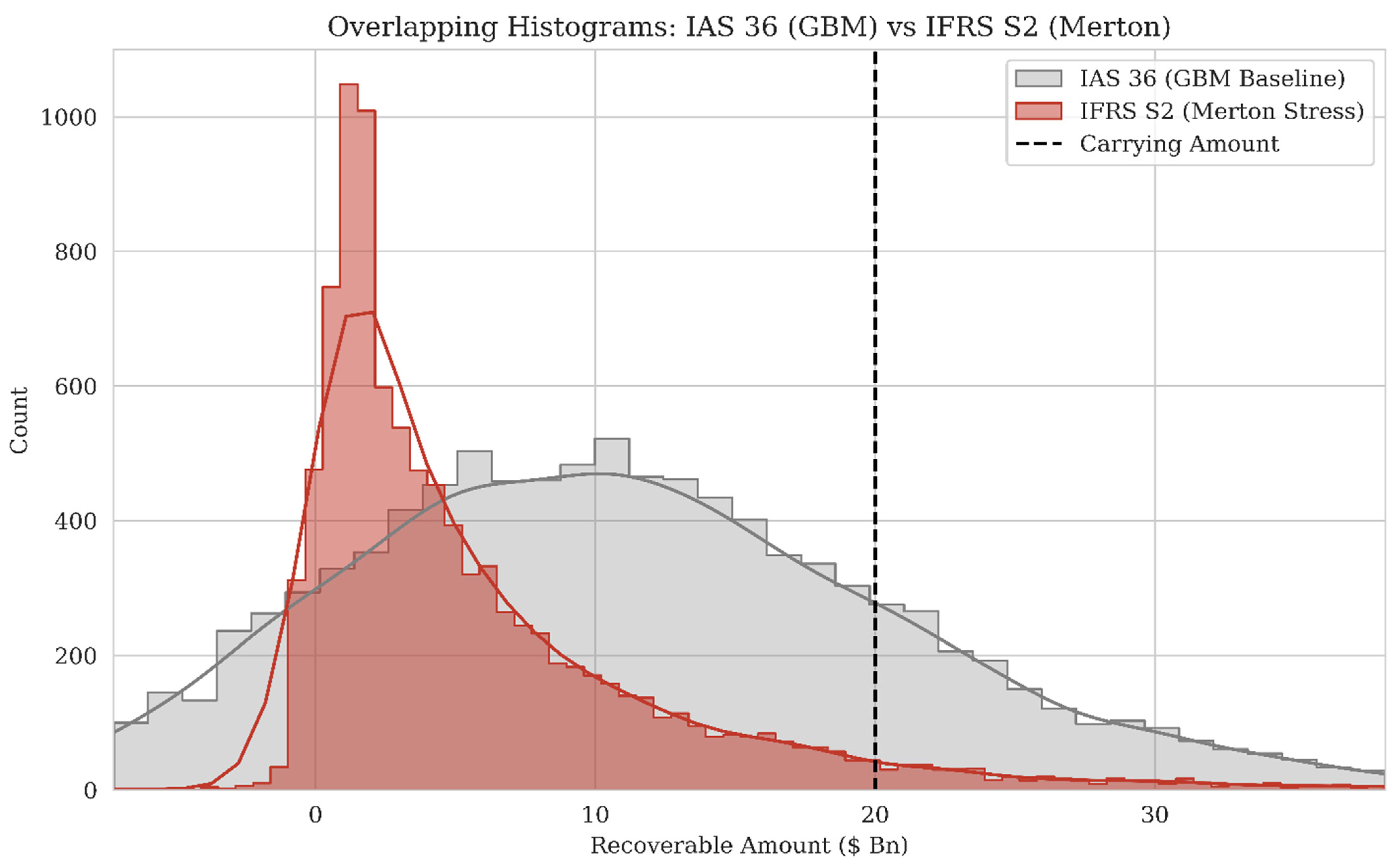
Distributional Shape and Tail Risks (Figure 1). As illustrated in Figure 1, the probability distribution exhibits a marked transformation. The IAS 36 distribution follows a relatively symmetric, bell-shaped curve (Skewness: 0.50). Conversely, the IFRS S2 distribution is heavily asymmetric, exhibiting pronounced positive Skewness (3.77) and elevated Kurtosis (33.69).

Figure 1 visually confirms the Green Swan phenomenon. As illustrated by the leftward concentration of the histogram (see highlighted region), the distribution’s probability mass shifts markedly toward lower values, indicating a substantially higher likelihood of failure. At the same time, the extended right tail (also visible in the figure) reflects the presence of rare but extreme positive outcomes, consistent with a fat-tailed distribution.

Regarding tail risks, the Value at Risk (VaR at the 95% level) and Conditional Value at Risk (CVaR at the 95% level) under the IFRS S2 scenario appear numerically smaller (i.e., closer to zero, at −0.19 Bn and −0.76 Bn, respectively) than in the baseline scenario. This seemingly counterintuitive result is explained by the model’s stranding mechanism. Unlike the GBM framework, which allows negative values to drift indefinitely, the IFRS S2 specification incorporates an economic stop-loss (i.e., abandonment) once cash flows become persistently negative.

Importantly, the visual features highlighted in Figure 1, namely the leftward shift and truncated downside, are fully consistent with this mechanism. However, this lower bound on losses provides limited economic reassurance, as the Probability of Impairment rises sharply to 94.47%, indicating that although extreme losses are capped, the likelihood of incurring impairment is near certain.

4.2. Scenario Analysis: The Mechanics of Value Erosion

To deconstruct the drivers of this devaluation, Table 8 presents the results of specific stress scenarios designed to isolate the impact of key transition variables.

Table 8. Scenario Analysis and Stress Testing: Impact of Transition Shocks on Value Erosion and Stranding Probability.

Scenario	Mean VIU ($Bn)	Change (%)	Stranding (%)	Impairment (%)
IAS 36 (GBM Baseline)	11.16	0.00%	0.00%	81.33%
IFRS S2 (Merton Stress)	6.27	−43.77%	98.85%	94.47%
Stress 1: Zero Pass-Through	5.07	−54.53%	99.75%	96.80%
Stress 2: Double Volatility	8.34	−25.25%	94.25%	88.10%
Stress 3: Aggressive Jumps	2.02	−81.86%	100.00%	99.60%
Stress 4: WACC Shock (+2%)	5.88	−47.29%	99.15%	95.35%

Table 8. Scenario Analysis and Stress Testing: Impact of Transition Shocks on Value Erosion and Stranding Probability.

Scenario	Mean VIU ($Bn)	Change (%)	Stranding (%)	Impairment (%)
IAS 36 (GBM Baseline)	11.16	0.00%	0.00%	81.33%
IFRS S2 (Merton Stress)	6.27	−43.77%	98.85%	94.47%
Stress 1: Zero Pass-Through	5.07	−54.53%	99.75%	96.80%
Stress 2: Double Volatility	8.34	−25.25%	94.25%	88.10%
Stress 3: Aggressive Jumps	2.02	−81.86%	100.00%	99.60%
Stress 4: WACC Shock (+2%)	5.88	−47.29%	99.15%	95.35%

The scenario analysis yields critical insights into the Managerial Myopia phenomenon (An et al., 2025).

First, Stress 1 (Zero Pass-Through) demonstrates that the loss of pricing power is a critical driver of value destruction for carbon-intensive assets. If the firm is unable to pass carbon costs to customers, due to market competition or carbon leakage, the valuation drops to $5.07 billion (−54.5%), pushing the impairment probability to 96.8%. This challenges the static margin assumptions often utilized in impairment tests.

Second, Stress 3 (Aggressive Jumps) illustrates the severe impact of disorderly transition policies. When the frequency of regulatory shocks $\begin{array}{c}\left(\lambda \right)\end{array}$ increases to 1.0 (one shock per year) with high magnitude, the mean asset value contracts sharply to $2.02 billion (−81.9%). This level is proximate to the scrap value, confirming that in a disorderly transition, legacy assets face existential valuation risks.

Notably, Stress 2 (Double Volatility) results in a less severe valuation drop ($8.34 billion) compared to the base stress scenario. This result is consistent with Real Options Theory (Castillo Delgadillo & Díaz-Peña, 2025). Higher volatility increases the option’s value during periods of high commodity prices, which mathematically raises the mean valuation. However, the stranding probability remains critically high at 94.25%, indicating that while volatility may offer upside potential in rare instances, it does not mitigate the fundamental solvency risk.

4.3. Sensitivity and Correlation Analysis: Unpacking the Drivers

To further validate the model’s internal consistency, we examined the correlation between the input parameters and the resulting valuation.

Table 9. Correlation Matrix between Stochastic Climate Drivers and Recoverable Amount.

Parameter	Pearson Correlation	Spearman Correlation
Sigma (Volatility)	0.11	0.12
Lambda (Jump Intensity)	−0.34	−0.33
Kappa (Mean Reversion)	−0.27	−0.24
WACC (Discount Rate)	−0.26	−0.23

reports the Pearson and Spearman correlations derived from the Monte Carlo iterations.

The analysis reveals a distinct negative correlation between Lambda $\begin{array}{c}\left(\lambda \right)\end{array}$ and valuation (Pearson: −0.34). This statistically validates the detrimental nature of discontinuous policy shocks. Unlike continuous volatility $\begin{array}{c}\left(\sigma \right)\end{array}$, which shows a weak positive correlation due to the aforementioned option value effect, the arrival of discrete jumps in carbon prices systematically destroys value by permanently elevating the cost structure. This result highlights that continuous volatility and discontinuous shocks represent distinct dimensions of risk, with materially different implications for valuation outcomes.

Furthermore, Table 10 (Tornado Analysis) ranks the variables by their marginal impact on the valuation range.

Table 10. Sensitivity Analysis (Tornado): Hierarchical Ranking of Variables by Financial Impact Range.

Parameter	Low Case ($Bn)	High Case ($Bn)	Base ($Bn)	Range ($Bn)
WACC	6.96	6.05	6.27	0.91
Jump Size	6.68	6.19	6.27	0.49
Lambda	6.41	6.02	6.27	0.39
Sigma Carbon	6.10	6.45	6.27	0.35

Table 10. Sensitivity Analysis (Tornado): Hierarchical Ranking of Variables by Financial Impact Range.

Parameter	Low Case ($Bn)	High Case ($Bn)	Base ($Bn)	Range ($Bn)
WACC	6.96	6.05	6.27	0.91
Jump Size	6.68	6.19	6.27	0.49
Lambda	6.41	6.02	6.27	0.39
Sigma Carbon	6.10	6.45	6.27	0.35

The Weighted Average Cost of Capital (WACC) emerges as the most sensitive parameter, with a range impact of $0.91 billion. This heightened sensitivity to the discount rate is characteristic of distressed assets; when future cash flows are marginal, the present value becomes disproportionately responsive to the cost of capital. This suggests that rising interest rates or climate-risk premia could accelerate asset stranding.

4.4. Stranding Risk and the Tipping Point

Finally, we address Hypothesis 2 regarding the probability of asset stranding. Stranding is defined here as the occurrence of two consecutive years of negative Free Cash Flow, necessitating economic abandonment. Table 11 reports the evolution of this probability as a function of climate-shock frequency (λ), thereby allowing a direct assessment of the role of discontinuous transition dynamics.

Table 11. Evolution of Stranding Risk in Relation to Regulatory Shock Intensity $\begin{array}{c}\left(\mathbf{\lambda }\right)\end{array}$.

Lambda (λ)	Frequency Interpretation	Stranding Prob (%)
0.0	No Shocks (Stable)	94.20%
0.2	Low (1/5 yrs)	96.58%
0.5	Medium (1/2 yrs)	99.24%
0.8	High (1/1.25 yrs)	99.76%
1.0	Extreme (1/1 yr)	99.90%

Table 11. Evolution of Stranding Risk in Relation to Regulatory Shock Intensity $\begin{array}{c}\left(\mathbf{\lambda }\right)\end{array}$.

Lambda (λ)	Frequency Interpretation	Stranding Prob (%)
0.0	No Shocks (Stable)	94.20%
0.2	Low (1/5 yrs)	96.58%
0.5	Medium (1/2 yrs)	99.24%
0.8	High (1/1.25 yrs)	99.76%
1.0	Extreme (1/1 yr)	99.90%

Table 11 reveals a strong monotonic relationship between jump intensity (λ) and stranding probability. These results reflect the combined effect of baseline volatility and constrained pass-through assumptions, rather than the absence of transition pressure.

The empirical evidence further indicates that even in a No Shocks scenario (λ = 0), the stranding probability under IFRS S2 conditions remains high at 94.20%. This suggests that the combination of limited pass-through capability (40%) and elevated baseline volatility renders the current BF-BOF technological route structurally fragile, even in the absence of discrete policy shocks. Accordingly, the asset may become economically obsolete under baseline transition assumptions.

Collectively, these results provide a quantitative basis for the Constructive Accounting framework proposed in this study. The $4.89 billion gap is not merely a measurement variance but a reflection of the methodological divergence between the accounting construct of stability and the economic reality of disruption. By relying on deterministic models (IAS 36), auditors may inadvertently validate valuations that have a negligible probability of realization in a Net Zero scenario. This confirms that the Connectivity Gap represents a form of regulatory arbitrage, allowing firms to defer the recognition of technological obsolescence.

5. Conclusions

The primary objective of this study was to operationalize and quantify the Connectivity Gap between the deterministic logic embedded in IAS 36 impairment testing and the stochastic nature of climate transition risks disclosed under IFRS S2. By constructing a Synthetic Representative Firm (SRF) within the European steel sector and subjecting its valuation to Monte Carlo simulation under a Merton Jump-Diffusion specification, the analysis moves beyond conceptual debate. It provides a quantitative assessment of how alternative stochastic assumptions affect recoverable amount estimates. The findings indicate that separating sustainability risk disclosures from financial measurement assumptions may lead to materially different valuation outcomes, with direct implications for capital allocation and long-term solvency assessments.

The simulation results document a $4.89 billion Sustainability Discount, corresponding to a 43.8% reduction in the recoverable amount when shifting from continuous growth assumptions typical of deterministic IAS 36 modeling ($11.16 billion) to discontinuous transition scenarios aligned with IFRS S2 ($6.27 billion). This divergence reflects the sensitivity of impairment outcomes to jump intensity (λ) and volatility (σ) parameters embedded in carbon price dynamics. Under the calibrated assumptions, the probability distribution of valuation outcomes shifts materially, suggesting that deterministic specifications may underrepresent left-tail exposure in Net-Zero scenarios.

From a methodological perspective, the study demonstrates how Constructive Accounting can be operationalized through formal stochastic modeling. Rather than representing unnecessary complexity, the integration of jump-diffusion dynamics within the Value-in-Use framework aligns the measurement architecture with the economic characteristics of climate transition risk. Moving from single-point estimates to probabilistic distributions enhances representational faithfulness as articulated in the Conceptual Framework and provides a structured mechanism for linking Double Materiality disclosures to impairment measurement.

While the Sustainability Discount reflects a reduction in expected asset value due to transition risk, it should not be interpreted solely as value destruction. Rather, it represents a re-pricing of risk under alternative stochastic assumptions, which may be partially mitigated through strategic adaptation. It may also function as a strategic signal. Adjustments in technological adoption and operational strategy, such as digital optimization and Circular Carbon Economy initiatives, can influence underlying risk parameters by reducing carbon exposure, lowering volatility (σ), and mitigating policy shock intensity (λ). Within the simulation environment, such parameter adjustments partially recover valuation losses, illustrating how transition risk management may alter impairment trajectories over time.

The findings offer implications for standard setters, auditors, and practitioners. Regulators may find that narrative disclosure alone is insufficient to capture the valuation sensitivity associated with stochastic transition risk. Incorporating scenario-based quantitative ranges within impairment analysis could enhance transparency and comparability. Meanwhile, the analysis underscores for auditors the importance of critically evaluating the stochastic assumptions embedded in management’s projections, particularly in carbon-intensive sectors where regulatory shocks may materially affect recoverable amounts.

While the study focuses on the European steel sector because of data availability and the maturity of the EU-ETS, the modeling framework is adaptable to other capital-intensive industries. Nevertheless, several limitations should be acknowledged. First, regarding sample scope, the SRF is constructed from large-scale BF-BOF producers within the EU-ETS and CBAM regulatory environment. The findings may not directly generalize to small- and medium-sized enterprises, firms employing exclusively Electric Arc Furnace (EAF) technology, or jurisdictions operating under different carbon pricing mechanisms, such as China’s national carbon market or North America’s carbon border adjustment proposals (Han et al., 2025). The applicability boundaries of the framework are therefore defined by the geographical (EU/EEA), enterprise-size (Tier-1 producers), and technological route (integrated BF-BOF) parameters of the SRF construction. As such, the magnitude of the Sustainability Discount identified in this study may represent an upper-bound estimate for large integrated producers rather than an industry-wide average. The calibration of jump intensity (λ) and volatility (σ) relies on historical carbon market behavior and NGFS-aligned scenarios; parameter estimates may therefore be sensitive to future policy regime shifts. The Synthetic Representative Firm abstracts from firm-level heterogeneity in financing structure and operational flexibility. Second, this study focuses exclusively on transition risks as defined under IFRS S2 (carbon pricing, regulatory shocks, and technological obsolescence). Physical climate risks, which are also required under IFRS S2 disclosure, include production disruptions caused by extreme weather events, supply chain interruptions, and direct asset damage, and are not incorporated into the current model. Physical risks could plausibly be modeled as additional Poisson jump components affecting production volume or fixed cost parameters, and their omission may understate the total climate-related impairment exposure. The decision to focus on transition risk reflects the study’s methodological objective of isolating the impact of carbon pricing discontinuities on asset valuation, but a comprehensive IFRS S2-aligned impairment framework would require integrating both risk categories. Future research could extend the framework to emerging-market contexts, incorporate physical risk as an additional jump component, and model endogenous investment adjustments to examine how green capex moderates the long-term probability of impairment.

Ultimately, integrating IFRS S2-related transition risk into IAS 36 impairment testing is not merely a compliance exercise but a measurement challenge under uncertainty. The Connectivity Gap identified in this study is economically material within the calibrated environment and highlights the importance of aligning valuation assumptions with the stochastic characteristics of climate transition dynamics, particularly in carbon-intensive industries. Strengthening this alignment enhances the decision usefulness of financial statements in a context where transition risk increasingly shapes asset valuation.