Do Environmental Taxes Stimulate Eco-Investments? Evidence from Seven EU Member States and the EU-27

Abstract

The European Green Deal places environmental taxation at the centre of decarbonisation policies. Nevertheless, empirical evidence of its effectiveness as a stimulus for capital eco-investments remains limited, particularly at the sectoral level. The present study analyses this relationship through a country–sector panel of seven EU countries and four NACE Rev.2 sectors for the period 2014–2023. A six-step empirical strategy is employed, comprising: preliminary diagnostic tests (cross-sectional dependence, stationarity, cointegration), descriptive statistics, correlation analysis with relative indicators, fixed-effects panel regressions with control variables, a Granger causality test, and nine robustness checks. All monetary values are in real prices (base year 2015). The results reveal a clear scale effect—the correlation between the absolute values of environmental taxes and eco-investments is very high, but after normalisation by sectoral GVA it becomes practically zero and statistically insignificant. The panel regressions also find no statistically significant relationship, and the Granger test does not confirm causality in either direction. The addition of control variables (eco-expenditures, GVA growth) and sector interaction effects does not alter the result. Nine robustness checks confirm the stability of these findings. Within the sample under consideration, the analysis finds no robust direct relationship between environmental taxes and sectoral eco-investments. The results obtained suggest a need to rethink policy through a more targeted use of revenues, sectoral differentiation, and combining tax instruments with non-fiscal mechanisms for the more effective management of the financial risk of the transition.

1. Introduction

The European Green Deal sets the ambitious goal for the EU to become climate-neutral by 2050. This transition requires significant capital investment in clean technologies and environmental protection—but also entails new financial risks. Companies face the so-called transition risk—the financial risk associated with changing regulations, tax rates, technological standards, and market preferences that accompany the ecological transition (TCFD, 2017; ECB, 2020). One of the key instruments of this transition is environmental taxation.

Environmental taxes—taxes on energy, transport, pollution, and resources—are a fiscal instrument grounded in Pigouvian logic. By raising the price of pollution, they are intended to stimulate enterprises to invest in cleaner technologies (Pigou, 1920; Baumol, 1972). The theoretical logic is compelling, but the empirical question remains open—to what extent this mechanism manifests itself in practice in the form of real investments in environmental protection.

The existing literature provides an ambiguous answer. Some studies find a positive relationship between environmental taxation and environmental performance, such as reduced emissions (Andersson, 2019; Sen & Vollebergh, 2018) or eco-innovations (Acemoglu et al., 2012). Others show that the effect depends on the tax burden, the institutional environment, and sectoral specifics (Dechezleprêtre & Sato, 2017; Marin & Vona, 2021). Studies that use sectoral panel data to trace the direct relationship between environmental taxes and capital eco-investments remain limited. Most analyses work with aggregated national data, which makes it difficult to capture significant sectoral differences—and it is precisely these that are of key importance for managing the financial risk of the ecological transition.

The green transition does not proceed uniformly across all economies and sectors. The greatest differences manifest precisely where energy, resource, and environmental pressures are strongest. In such an environment, the aggregate national perspective may create an apparent impression of a unidirectional stimulating effect of environmental taxes, whereas at the country–sector level, differences related to scale, structure, and adaptive capacity become evident.

On this basis, the study uses a country–sector panel of seven countries and four sectors according to NACE Rev.2 for the period 2014–2023 to answer the following research question: does a statistically significant relationship exist between environmental taxes and capital eco-investments at the sectoral level in the EU? The contribution of the article is that it shifts this debate from the level of aggregated national indicators to a country–sector analysis and shows that within the sample under consideration no statistically significant direct tax investment effect is established. The low explanatory power of the models (within R² below 3%) additionally suggests that investment decisions at the sectoral level are likely determined to a greater extent by broader structural factors than by the tax stimulus itself. In this sense, the result calls into question the assumption of a simple and direct mechanism whereby tax pressure automatically translates into an investment stimulus, and points to the need for a policy mix in which tax instruments are combined with additional regulatory, financial and institutional measures.

From this, the following three hypotheses arise:

H1. 

Higher environmental taxes are associated with higher capital eco-investments at the sectoral level.

H2. 

The relationship between environmental taxes and capital eco-investments differs across sectors.

H3. 

Capital eco-investments depend not only on environmental taxes but also on macroeconomic growth and current environmental expenditures.

2. Literature Review

2.1. Theory of Environmental Taxation

The theoretical framework of environmental taxation is grounded in Pigou’s concept (Pigou, 1920). According to it, taxes on pollution correct negative externalities by aligning private costs with social costs. Baumol (1972) further develops this idea by proposing a practically applicable variant of the Pigouvian approach, in which the tax serves to achieve a pre-set environmental standard. The main mechanism is clear—a higher price of pollution creates an incentive for firms to invest in cleaner technologies, thereby simultaneously reducing emissions and limiting future costs.

The Porter Hypothesis (Porter & van der Linde, 1995) extends this argument. According to it, well-designed environmental regulations can not only stimulate innovation but also enhance the competitiveness of firms. The double dividend hypothesis (Goulder, 1995) adds a further dimension, according to which revenues from environmental taxes can replace distortionary taxes, which would deliver both environmental and economic benefits simultaneously.

This outcome, however, is not automatic. Bovenberg and de Mooij (1994) emphasise that in a real-world setting with multiple taxes and market distortions, the net effect may be weaker than expected. More recent studies also show that results vary substantially depending on the specific design of the tax, the method of measuring regulation, and the institutional environment of implementation (Köppl & Schratzenstaller, 2023; Zhang et al., 2024).

An important distinction in the literature is between tax revenues and tax incentives. Revenues from environmental taxes reflect not only the tax rate but also the volume of output, price effects, and changes in the tax base. Köppl and Schratzenstaller (2023) emphasise that using revenues as a proxy for policy stringency may lead to misleading conclusions, since higher revenue may indicate a greater volume of taxable activity rather than necessarily a stronger tax signal. This distinction is key for the present study and requires careful interpretation of tax revenues as an indicator of tax pressure.

2.2. Innovation and Investment Responses to Environmental Taxes

The empirical literature distinguishes three channels of impact of environmental taxes—on emissions, on innovation, and on real capital investments. The distinction between them is essential, since a positive effect in one direction does not automatically imply a similar effect in another.

The most extensively studied is the effect on greenhouse gas emissions and pollution. Andersson (2019), using the synthetic control method, shows that the carbon tax in Sweden leads to a reduction in transport CO₂ emissions of approximately 11%. Sen and Vollebergh (2018), through instrumental variables, find that an increase in energy taxes of 1 euro is associated with a 0.73% decrease in carbon emissions in the long run. Wolde-Rufael and Mulat-Weldemeskel (2023) also confirm a negative relationship between environmental taxes and CO₂ emissions in 20 European countries. Similar conclusions are drawn by Bretschger and Grieg (2024) for the United Kingdom, where higher fuel taxation reduces transport CO₂ emissions without a clearly pronounced negative effect on economic activity. Kohlscheen et al. (2025) also find a statistically significant reduction in CO₂ emissions, particularly in the long run.

Nevertheless, the empirical results are not entirely unambiguous. Morley (2012) finds an effect on pollution but not on energy consumption, which points towards a technological transition rather than a contraction of consumption. Liobikienė et al. (2019), Silajdžić and Mehić (2018), as well as Godawska (2024) also report limited or heterogeneous effects. Consequently, the evidence for an effect on emissions is comparatively stronger but remains sensitive to the specific design of the tax, the sample, and the method employed.

The effect on innovation is more indirect. Acemoglu et al. (2012) develop a model of directed technical change, according to which taxes and subsidies can redirect innovative efforts from “dirty” to “clean” technologies. Aghion et al. (2016) confirm this empirically in the automotive industry. Similar results are reported by other studies showing that environmental policies and price incentives encourage low-carbon innovations (Johnstone et al., 2010; Calel & Dechezleprêtre, 2016; Feng et al., 2024; Hu et al., 2025). At the same time, the literature shows that the effect also depends on the type of instrument employed—tax, subsidy, standard, or a combination thereof (Johnstone et al., 2010; Palage et al., 2019; Hille et al., 2020; Blagoeva & Georgieva, 2023). This indicates that environmental taxes can direct technological change, but this effect does not automatically translate into immediate capital investments.

The least studied question remains whether environmental taxes translate into real capital eco-investments. Popp (2002) and Jaffe and Palmer (1997) show that higher energy prices stimulate patenting and R&D expenditures, but the evidence for a real investment effect is weaker—firms respond first with technological preparation rather than with immediate capital outlays. Benatti et al. (2024) also confirm that environmental regulations stimulate clean innovations, but the effect is significantly stronger in combination with direct R&D subsidies. Particularly indicative is the study by Carfora et al. (2021), according to which the tax burden may act as a barrier to investments in RES in the EU, whereas targeted support policies, such as feed-in tariffs, have a positive effect. This suggests that tax pressure and investment stimulus are not the same thing.

2.3. Sectoral Heterogeneity

Sectoral heterogeneity is key to assessing the effect of environmental taxes, since individual industries differ in energy intensity, technological structure, regulatory exposure, and the capacity for adaptation. This means that the same tax signal may provoke different responses depending on the sector.

Dechezleprêtre and Sato (2017) show in a systematic review that environmental regulations generate significant but limited short-term negative effects on competitiveness, primarily in energy-intensive and pollution-intensive sectors. Marin and Vona (2021) confirm with micro-data for French enterprises that the effect of energy prices depends on sectoral specifics and firm characteristics. Ambec et al. (2013) emphasise that positive outcomes are more likely with well-designed, predictable, and consistent policies. Calel and Dechezleprêtre (2016) also show that the EU ETS stimulates low-carbon innovations in regulated firms, but the effect depends on the specific instrument and the institutional environment.

Consequently, there is reason to expect that the impact of environmental taxes is not homogeneous but differs across sectors depending on their production profile, energy dependence, and adaptive capacity.

2.4. Climate Transition Risk and Sustainable Finance

The climate transition is increasingly viewed not only as an environmental but also as a financial challenge. The TCFD (2017) identifies four main categories of climate-related financial risks—regulatory, technological, market, and reputational, with environmental taxes falling within the group of regulatory risks. The ECB (2020) formulates expectations for banks to integrate climate risks into governance and disclosure, while Nerlich et al. (2025) emphasise the existence of a significant gap between the necessary and actually realised green investments in the EU. Battiston et al. (2017) show that such effects can propagate through the financial system and give rise to systemic risk.

The literature on sustainable finance further develops this perspective. NGFS (2022) develops climate transition scenarios that model the interaction between carbon pricing, investment behaviour, and financial stability. Regulation (EU) 2020/852 (European Parliament and Council of the European Union, 2020) (EU Taxonomy) creates a classification framework for environmentally sustainable activities and influences investment decisions through disclosure requirements. Krastev and Krasteva-Hristova (2024) also note that tax policy in itself is not sufficient if it is not combined with regulatory predictability and broader changes in the financial environment. This suggests that the effect of environmental taxes depends on a combination of additional regulatory, financial, and institutional factors.

This perspective is also important for the interpretation of the results. The absence of a direct relationship between taxes and eco-investments does not necessarily mean that tax policy is insignificant. It is possible that its effect manifests indirectly—through cost pressure, a change in the risk profile, technological deferral, or the redirection of investments. This is precisely why the empirical verification of the direct relationship remains necessary.

In this sense, the literature on climate financial risk and the literature on environmental taxation converge on a common question—not simply whether the policy is “green” but whether it is effective as a mechanism for real adaptation. The present study is positioned precisely at this intersection between the fiscal instrument, investment behaviour, and risk management in the context of the green transition.

2.5. Literature Gaps and Contribution of the Study

The literature review outlines three main gaps. First, most studies focus on emissions rather than on capital eco-investments, which is why the relationship between environmental taxes and the real investment response remains under-researched. Second, relatively few studies combine a cross-country and cross-sector dimension, despite the fact that sectoral differences are substantial and the same tax pressure may act as a stimulus in one sector and as a barrier in another. Third, the predominant use of absolute values without controlling for the scale of the economy may lead to systematically misleading conclusions.

The present study addresses these gaps through a country–sector panel of seven countries and four NACE sectors for the period 2014–2023. Its contribution lies in combining a cross-country and cross-sector dimension, using relative rather than solely absolute indicators, and placing the focus on capital eco-investments as a direct expression of adaptation to the green transition. In this way, the study assesses not simply whether environmental taxes are associated with better environmental outcomes but whether they function as an effective financial stimulus for real investment adaptation in the context of transition risk. By documenting the absence of a robust direct relationship, the study provides an empirical basis that environmental taxes, considered in isolation, may be insufficient for stimulating sectoral capital investments. This underscores the importance of complementary policy instruments—subsidies, regulatory incentives and the targeted use of tax revenues—for achieving a real investment response.

3. Materials and Methods

3.1. Data and Sample

The study uses panel data extracted from the publicly available databases of Eurostat. The sample covers seven EU member states (Belgium, Bulgaria, France, Hungary, Italy, Poland, and Romania), with EU-27 as a reference aggregate for the descriptive analysis. The selection of countries aims to ensure geographical and economic diversity, including old and new EU members, larger and smaller economies, as well as Western and Eastern European countries. The selection is also conditioned by data availability. Data on environmental investments by NACE sectors (env_ac_epiap1) became mandatory for reporting only from 2017 pursuant to Commission Delegated Regulation (EU) 2022/125 (European Commission, 2022), and for the period 2014–2016 most countries did not provide complete series. The seven countries indicated are the only ones for which continuous data are available for the four analysed sectors for the entire period 2014–2023.

The panel is structured by countries, sectors, and time. Each observed unit represents a combination of country and sector, tracked for the period 2014–2023. Four NACE Rev. 2 sectors are covered: A—agriculture, forestry, and fishing; B—mining and quarrying; C—manufacturing; D—energy. This forms a balanced panel of 280 observations (7 countries × 4 sectors × 10 years), or 320 when EU-27 is included. EU-27 is used solely in the descriptive analysis as a reference value but does not participate in the econometric estimations, in order to avoid double counting and artificial amplification of the scale effect. For this reason, the regression models are estimated on 280 observations.

All monetary values are recalculated in real prices with a base year of 2015 using the GDP implicit price deflator in euros (PD15_EUR, Eurostat, nama_10_gdp). Deflation is necessary because the period 2014–2023 encompasses significant inflationary and energy price shocks, particularly after 2021, which could distort both the descriptive and regression results when working with current prices.

3.2. Variables

Table 1. Variable descriptions.

Variable	Abbrev.	Description	Eurostat Code	Unit	Rationale
Dependent variable
Eco-investment	EcoInvest	GFCF for environmental protection by NACE sector (ancillary producers)	env_ac_epiap1	million EUR real 2015	Reg. 691/2011; Carfora et al. (2021)
Independent variables
Env. taxes	EnvTax	Environmental tax revenue by NACE sector	env_ac_taxind2	million EUR real 2015	Reg. 691/2011; Morley (2012)
Control variables
Eco-expenditure	EcoExpend	Current expenditure on env. protection (proxy for OPEX)	env_ac_cepsgc1	million EUR real 2015	EPEA methodology
GVA	VA	Gross value added by sector	nama_10_a10	million EUR real 2015	Eurostat NA
GDP	GDP	Gross domestic product	nama_10_gdp	million EUR real 2015	Eurostat NA
VA growth	ΔVA%	Annual real GVA growth rate	Computed	%	Macro control
Derived indicators
Invest. intensity	InvInt	EcoInv/sectoral GVA	Computed	%	Scale-adjusted
Tax intensity	TaxInt	EnvTax/sectoral GVA	Computed	%	Scale-adjusted
Exp. intensity	ExpInt	EcoExp/sectoral GVA	Computed	%	Control ratio
Lagged tax	EnvTaxt−1	Env. taxes at t − 1 (absolute and intensity)	Computed	var.	Delayed response

Source: Author’s calculations.

presents the variables used. The dependent variable is eco-investments (EcoInvest), measured as gross fixed capital formation for environmental protection under the EPEA (Environmental Protection Expenditure Accounts) methodology pursuant to Regulation (EU) 691/2011 (European Parliament and Council of the European Union, 2011). The data are taken from the dataset env_ac_epiap1 and cover enterprise investments by economic activities according to NACE Rev.2. This measure reflects capital expenditures for environmental protection, such as wastewater treatment facilities, air emission abatement, and waste management. It does not include investments in resource management, energy efficiency, renewable energy, research and development, and climate adaptation, unless they are directly related to environmental protection. For this reason, EcoInvest should not be interpreted as a measure of all investments in climate transition.

The main independent variable is environmental taxes (EnvTax), reported pursuant to Regulation 691/2011. They comprise four groups—energy taxes, transport taxes, pollution taxes, and resource taxes—distributed by economic activities according to NACE Rev.2. Tax revenues do not fully accurately measure the strength of the tax incentive, since they may change not only due to a change in the tax burden but also as a result of changes in output, prices, or the tax base. Therefore, the analysis uses both absolute values and a relative indicator—environmental taxes as a percentage of sectoral gross value added.

In the extended models, control variables are also included. EcoExpend reflects current non-investment expenditures for environmental protection and serves as an indicator of the current environmental burden of the sector. VA_growth measures the annual growth of real gross value added and captures overall economic dynamics. In addition, lagged values of the tax variables with a one-year delay are used to test for a possible delayed investment response.

Variables such as environmental subsidies, sectoral energy prices, and exposure to the EU ETS are not included in the model due to the lack of comparable data at the country × sector level in Eurostat for the period under consideration. Data on environmental subsidies became mandatory only from 2025. This limitation is taken into account in the interpretation of the results.

To eliminate the influence of economic scale, relative indicators are also used in the analysis—eco-investments and eco-taxes as a percentage of the gross value added of the respective sector. These indicators allow better comparability between units of different size and limit the risk of misleading correlations when working with absolute values. All monetary values are presented in millions of euros, in real prices with a base year of 2015.

3.3. Analytical Framework

The analysis follows a six-step strategy (

Table 2. Six-step empirical strategy.

Stage	Method	Purpose
1	Diagnostic pre-tests	Pesaran CD test (CSD); LLC and IPS unit root tests; Pedroni & Kao cointegration; VIF; Modified Wald (heteroskedasticity); Wooldridge (serial correlation)
2	Descriptive statistics	Characterise distributions, heterogeneity, and dynamics
3	Correlation analysis (Pearson)	Assess bivariate associations and examine scale effects
4	Panel regressions (FE, RE, Hausman)	Test the direct link controlling for unobserved specifics
5	Granger causality test	Examine directionality (taxes → investments and/or reverse)
6	Robustness checks	Confirm findings under alternative specifications (9 checks incl. deflated values, Winsorisation, alternative DV, sector interactions)

Source: Author’s calculations.

).

Before the estimation of the main models, diagnostic tests for cross-sectional dependence, stationarity, cointegration, multicollinearity, heteroscedasticity, and serial correlation were conducted. For this purpose, the Pesaran (2004) test, the Levin et al. (2002) and Im et al. (2003) tests, the Pedroni (1999) and Kao (1999) tests, VIF analysis, the modified Wald test (Greene, 2003), and the Wooldridge (2002) test were used. In view of the established heteroscedasticity and serial correlation, clustered standard errors by units are used in all models.

The correlation analysis uses the Pearson coefficient (r) to assess the linear relationship between the variables in both absolute and relative values. The main econometric instrument is a fixed-effects panel regression by units, which controls for unobserved and time-invariant characteristics of the units and identifies the effect through their within variation. The choice between fixed- and random-effects models is verified through the Hausman (1978) test.

Seven main specifications are used:

Model 1 (log-log): ln(EcoInvest_it) = α_i + β₁·ln(EnvTax_it) + β₂·ln(VA_it) + ε_it

(1)

Model 2 (intensity): InvInt_it = α_i + β₁·TaxInt_it + ε_it

(2)

Model 3 (FE + TE + lag): ln(EcoInvest_it) = α_i + γ_t + β₁·ln(EnvTax_i,t−1) + β₂·ln(VA_it) + ε_it

(3)

Model 4 (intensity + lag): InvInt_it = α_i + β₁·TaxInt_i,t−1 + ε_it

(4)

Model 5 (+controls): InvInt_it = α_i + β₁·TaxInt_i,t−1 + β₂·ExpInt_it + β₃·ΔVA%_it + ε_it

(5)

Model 6 (full): ln(EcoInvest_it) = α_i + γ_t + β₁·ln(EnvTax_i,t−1) + β₂·ln(VA_it) + β₃·ln(EcoExp_it) + ε_it

(6)

Model 7 (interactions): InvInt_it = α_i + Σ_k β_k·(TaxInt_it × Sector_k) + ε_it

(7)

where i denotes the unit (country–sector), t—the year, α_i—the unit fixed effect, γ_t—the time effect, and Sector_k—dummies for the four NACE sectors (k = A, B, C, D). All models use clustered standard errors (SEs) by units to correct for heteroscedasticity and autocorrelation within units. The choice of clustered SE is justified by the results of the modified Wald test (Greene, 2003) (p = 0.000 for heteroscedasticity) and the Wooldridge (2002) test (p = 0.032 for serial correlation). The choice between FE and RE is verified with the Hausman test (Hausman, 1978).

To verify the direction of the relationship, a panel Granger causality test (Granger, 1969) is applied, with both possible directions tested—from taxes to investments and vice versa. Due to the limited time dimension (T = 10), 1 and 2 lags are used.

The robustness checks include nine additional specifications—a random-effects model, a first differences model, exclusion of the years 2020–2021, separate estimates for new and old member states, a model with relative indicators and time fixed effects, a model with an alternative dependent variable that limits the influence of extreme values, and a model with an interaction between taxes and sector. These checks assess the sensitivity of the results to alternative assumptions, sub-samples, and specifications.

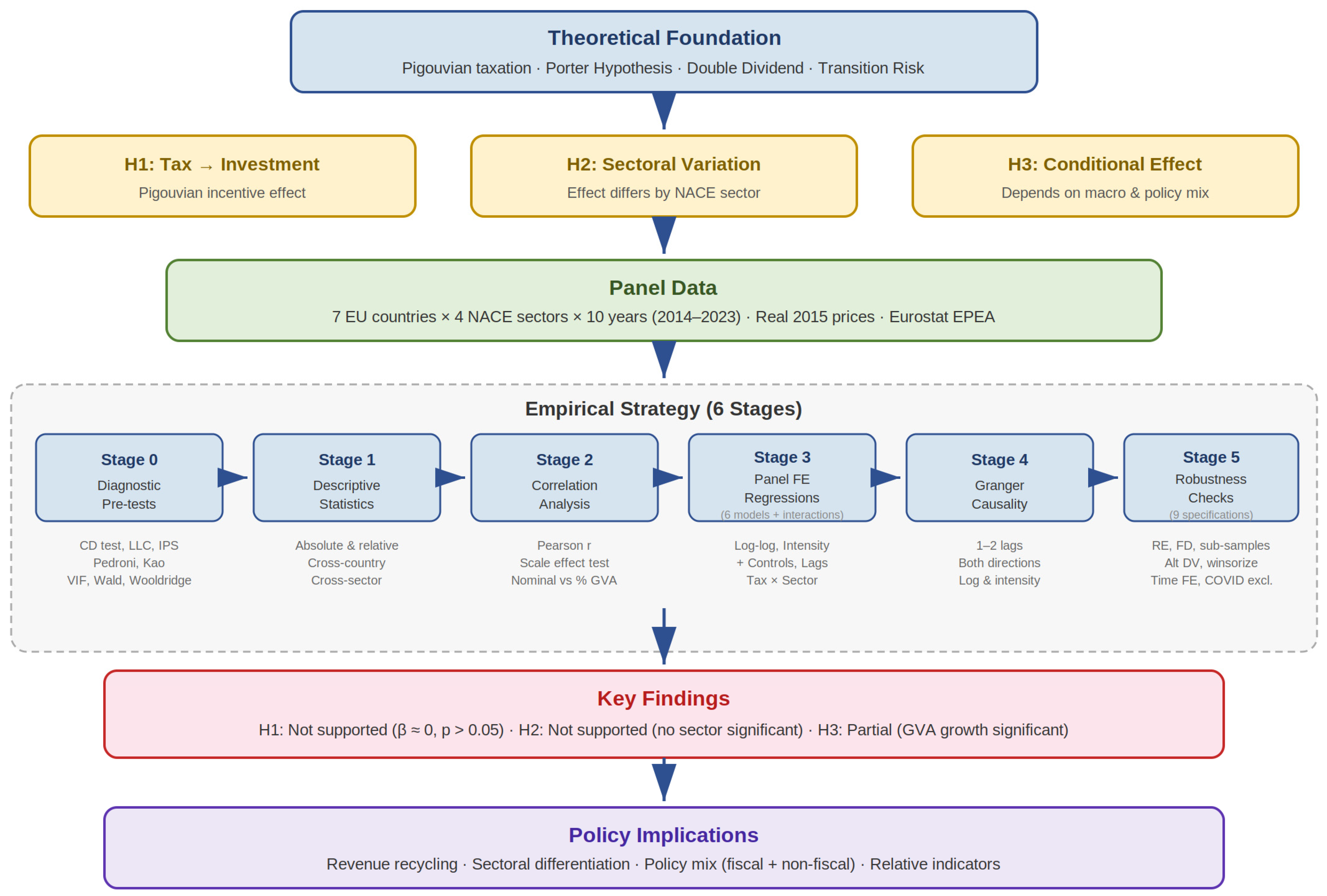
Figure 1 summarises the analytical framework of the study—from the theoretical basis and formulated hypotheses, through the data and the six-step empirical strategy, to the key findings and policy implications.

4. Results

4.1. Preliminary Diagnostic Tests

Before the main analysis, diagnostic tests were conducted to assess the panel properties of the data. Their results justify the choice of model specification and the use of corrected standard errors.

Cross-sectional dependence. The Pesaran (2004) test rejects the null hypothesis of no cross-sectional dependence for all key variables (

Table 3. Pesaran CD test for cross-sectional dependence.

Variable	CD Statistic	p-Value	Avg ρ	N	T	Decision
ln(Eco-Investment)	2.109	0.0349	0.037	26	10	Reject H0 (p < 0.05)
ln(Env. Taxes)	2.656	0.0079	0.043	28	10	Reject H0 (p < 0.01)
Invest. intensity (% VA)	2.881	0.004	0.051	28	10	Reject H0 (p < 0.01)
Tax intensity (% VA)	2.868	0.0041	0.047	28	10	Reject H0 (p < 0.01)
ln(GVA)	11.07	0	0.18	28	10	Reject H0 (p < 0.001)

Source: Author’s calculations.

). The CD statistic is significant at p < 0.05 for ln(EcoInvest) and at p < 0.01 for the remaining four variables. The dependence is most strongly pronounced for ln(VA) (CD = 11.07), which reflects common macroeconomic shocks affecting all countries and sectors simultaneously. These results necessitate caution in interpreting standard panel tests for stationarity and justify the use of clustered standard errors by units in all regression specifications.

Stationarity.

Table 4. Panel unit root tests (LLC and IPS).

Variable	LLC t-Stat	LLC p-Value	IPS t-Bar	IPS W-Stat	IPS p-Value	Conclusion
IN LEVELS
ln(Eco-Investment)	−8.741	0	−1.826	−1.703	0.0443	Stationary (both)
ln(Env. Taxes)	−8.262	0	−1.413	0.61	0.729	Mixed (LLC yes, IPS no)
Invest. intensity (% VA)	−12.296	0	−2.135	−3.423	0.0003	Stationary (both)
Tax intensity (% VA)	−7.798	0	−1.704	−1.044	0.1484	Mixed (LLC yes, IPS no)
ln(GVA)	−8.647	0	−1.828	−1.746	0.0404	Stationary (both)
IN FIRST DIFFERENCES
Δln(Eco-Investment)	−18.142	0	−3.157	−9.119	0	Stationary I(0)
Δln(Env. Taxes)	−21.835	0	−3.527	−11.386	0	Stationary I(0)
ΔInvest. intensity	−22.846	0	−3.41	−10.528	0	Stationary I(0)
ΔTax intensity	−15.459	0	−3.288	−10.031	0	Stationary I(0)
Δln(GVA)	−18.38	0	−3.202	−9.543	0	Stationary I(0)

Source: Author’s calculations.

presents the results of the Levin–Lin–Chu (LLC) and Im–Pesaran–Shin (IPS) tests for the presence of a unit root. In levels, the results are mixed—ln(EcoInvest), Invest intensity, and ln(VA) are stationary under both tests, while ln(EnvTax) and Tax intensity reject the unit root under LLC but not under IPS. In first differences, all variables are categorically stationary (p < 0.001). These results show that most variables are borderline I(0) or I(1), which justifies conducting cointegration tests.

Panel cointegration. The tests of Pedroni (1999) and Kao (1999) confirm the presence of cointegration between the key variable pairs (

Table 5. Panel cointegration tests (Pedroni & Kao).

Variable Pair	Pedroni ADF	Pedroni p-Value	Kao ADF	Kao p-Value	Conclusion
ln(EcoInvest) ~ ln(EnvTax)	−2.352	0.0001	−12.243	0	Cointegrated (both)
Invest_%VA ~ Tax_%VA	n/a	n/a	−14.631	0	Cointegrated (Kao)
ln(EcoInvest) ~ ln(VA)	−2.205	0.002	−9.993	0	Cointegrated (both)

Source: Author’s calculations.

). Both tests reject the null hypothesis of no cointegration between ln(EcoInvest) and ln(EnvTax), as well as between ln(EcoInvest) and ln(VA). This provides a basis for using regression specifications in levels, despite the mixed results from the stationarity tests. Taken together, these diagnostic results provide a basis for the chosen estimation strategy—the presence of cointegration permits working in levels, while the use of cluster-robust standard errors by unit accounts for cross-sectional dependence, heteroscedasticity and serial correlation. Additionally, robustness checks through first differences show that the results remain similar regardless of whether the models are specified in levels or in differences.

Regression diagnostics. The VIF analysis shows high multicollinearity between ln(EnvTax) and ln(VA) (VIF = 41.71), since both variables reflect the scale of the sector (

Table 6. Regression diagnostics summary.

Test	Statistic	p-Value	Conclusion
VIF: ln(EnvTax)	41.71	-	Severe (scale-driven)
VIF: ln(VA)	41.71	-	Severe (scale-driven)
VIF: EcoExp intensity	1.26	-	OK
Modified Wald (het.)	W = 403.0	0.000	Heteroskedasticity present
Wooldridge (serial corr.)	F = 4.65	0.032	Serial correlation present
Hausman M1 (log-log)	χ2 = 1.76	0.414	RE acceptable; FE preferred
Hausman M2 (intensity)	χ2 = 0.50	0.482	RE acceptable; FE preferred

Source: Author’s calculations.

). In the models with intensities (% of GVA), this problem is eliminated. Eco-expenditures as a control variable have VIF = 1.26—no multicollinearity problem. The modified Wald test rejects the hypothesis of homoscedasticity (W = 403.0, p = 0.000), and the Wooldridge test rejects the hypothesis of no serial correlation (F = 4.65, p = 0.032). For this reason, clustered standard errors by units (entity-clustered SE) are used in all subsequent models.

4.2. Descriptive Statistics and Trend Analysis

Table 7. Summary statistics of the key variables.

Variable	Mean	Std. Dev.	Min	Q1	Median	Q3	Max
Eco-investment (million euro)	624.75	1392.90	0.00	23.61	75.05	387.52	8675.32
Eco-expenditure (million euro)	2526.32	7612.74	0.00	3.56	90.95	698.97	45,058.12
Env. taxes (million euro)	2249.84	5769.61	6.30	85.78	344.84	1279.73	38,527.85
GVA (million euro)	102,535.67	339,557.09	141.79	2851.71	10,396.68	38,066.88	2,071,516.45
Eco-invest. (% of GVA)	1.40	2.09	0.00	0.28	0.71	1.43	12.19
Env. taxes (% of GVA)	4.04	3.99	0.19	1.75	3.03	4.87	32.21

Source: Author’s calculations based on Eurostat data.

shows that the observations in the panel are highly heterogeneous and are noticeably influenced by scale effects. The absolute values are in real prices (base 2015). The mean eco-investment per country–sector pair is EUR 624.75 million, but the typical value is considerably lower—the median is EUR 75.05 million. This divergence means that several very large observations (including the EU-27 aggregate and large economies such as France and Italy) dominate the distribution and raise the mean value. Consequently, mean values should be interpreted with caution, since they do not describe the “centre” of the data but are sensitive to extreme observations.

A similar picture is observed for environmental taxes—the mean value is EUR 2249.84 million with a median of EUR 344.84 million, which again suggests a concentration of volumes in a limited number of observations and the presence of pronounced right skewness.

The relative indicators provide a more comparable perspective, since they reduce the influence of size. In these terms, mean eco-investments are 1.40% of sectoral GVA, while environmental taxes are 4.04% of GVA. This ratio shows that within the panel, the tax burden (as a relative share) systematically exceeds the observed investment response, which motivates subsequent analysis of whether higher environmental taxes are associated with higher investment intensity.

Table 8. Mean values and growth dynamics by country (2014–2023).

Country	Eco-Invest. (Million Euro)	Eco-Expend. (Million Euro)	Env. Taxes (Million Euro)	Eco-Invest. (% of GVA)	Env. Taxes (% of GVA)	CAGR Invest. (%)	CAGR Taxes (%)
BE	148.27	308.88	384.76	2.57	4.40	+3.0	+3.8
BG	32.52	43.81	113.16	1.20	5.39	−7.2	+11.1
FR	1002.74	2048.77	1040.45	1.96	2.84	+2.3	+1.8
HU	29.70	73.81	149.27	0.58	2.65	−9.0	+5.1
IT	218.48	1913.68	2154.99	0.78	5.25	−10.0	−2.3
PL	254.40	0.00	838.56	1.51	2.37	−4.1	+8.6
RO	55.97	185.79	591.42	1.59	6.00	−13.6	−3.3
EU-27	3255.93	15,635.86	12,726.08	1.03	3.45	+1.1	+2.2

Source: Author’s calculations based on Eurostat data. CAGR = compound annual growth rate, 2014–2023.

outlines substantial cross-country differences. France stands out as the largest investor in absolute terms (mean EUR 1002.74 million), followed by Poland (EUR 254.40 million) and Italy (EUR 218.48 million). In relative terms, however, Belgium registers the highest investment intensity—2.57% of GVA—followed by France (1.96%) and Romania (1.59%). Hungary records the lowest intensity (0.58%), alongside the EU-27 aggregate (1.03%).

Particularly telling is the growth dynamics in real terms. Environmental taxes increase in most countries, with especially rapid growth in Bulgaria (CAGR: +11.1%), Poland (+8.6%), and Hungary (+5.1%), but in Italy (−2.3%) and Romania (−3.3%) they decline. Eco-investments contract in five of the seven national economies. Romania (−13.6%), Italy (−10.0%), and Hungary (−9.0%) record the sharpest declines, while Belgium (+3.0%) and France (+2.3%) report moderate growth. This asymmetry between rising tax burdens and declining investments in a number of countries raises initial questions regarding the effectiveness of environmental taxation as a stimulus for investment and necessitates in-depth econometric investigation.

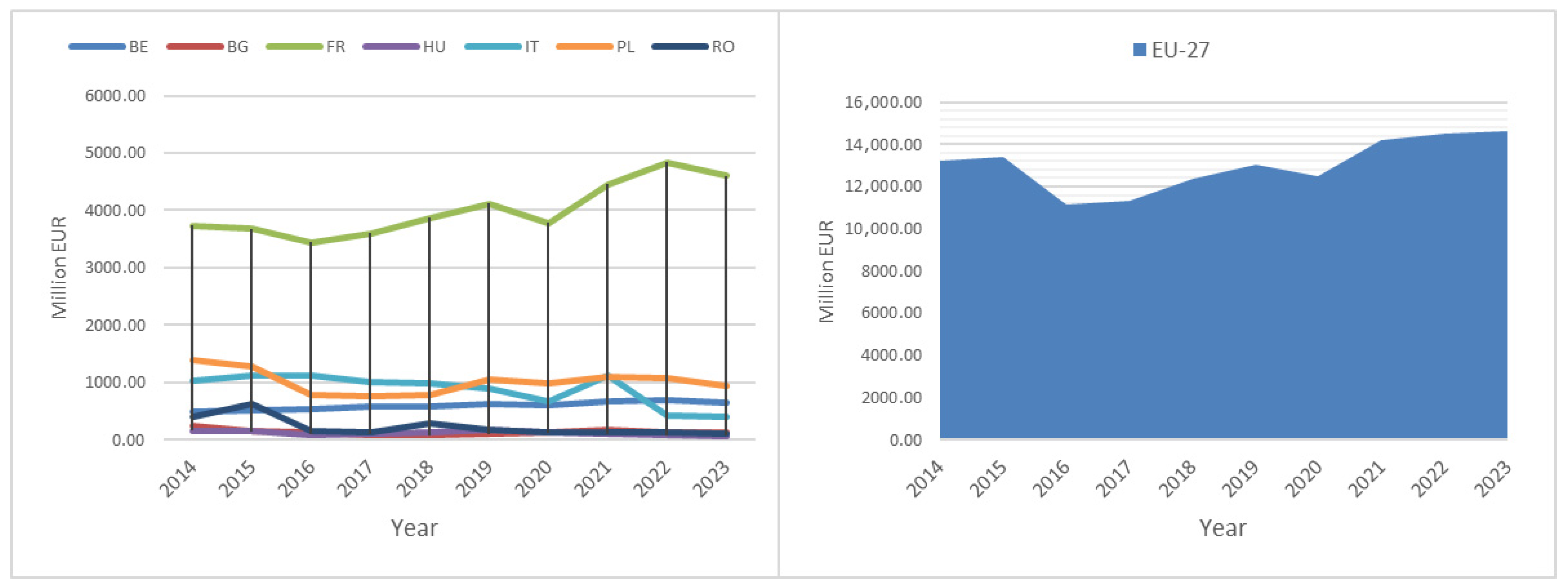
Figure 2 illustrates the temporal evolution of eco-investments in real prices (base 2015). Among national economies (left-hand panel), France shows a clear upward trajectory—from EUR 3737 million in 2014 to EUR 4834 million in 2022. Belgium follows a similar positive trend. Conversely, Italy registers a sharp decline—from EUR 1028 million (2014) to EUR 398 million (2023)—while Poland and Romania show fluctuating patterns without a clear direction. At the EU-27 level, total eco-investments increase from EUR 13,225 million in 2014 to EUR 14,605 million in 2023, representing cumulative growth of 10.4% (CAGR: +1.1%). The slight decline in 2020 most likely reflects the economic disruptions caused by the COVID-19 pandemic, although this is not tested directly in the model.

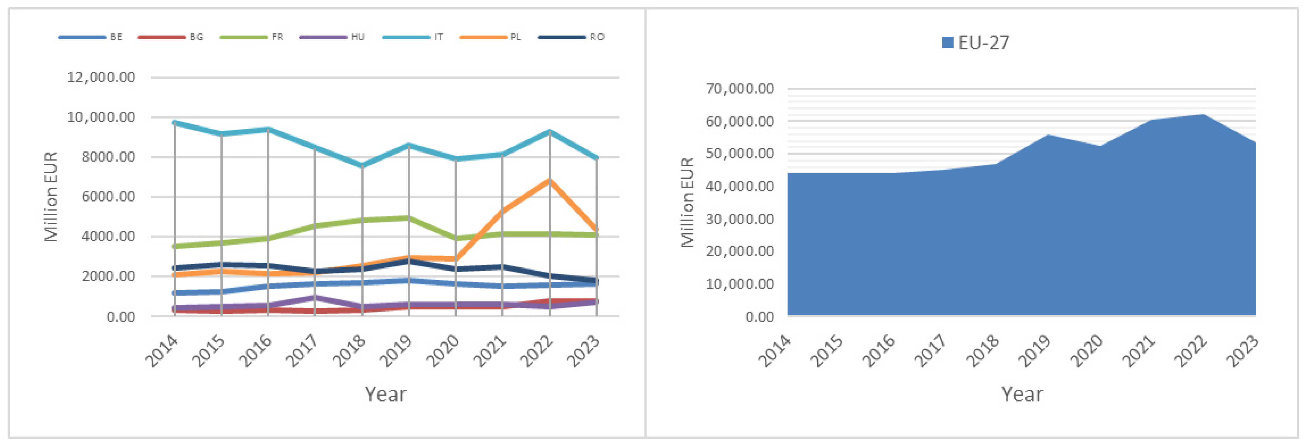
Figure 3 presents the corresponding trajectory of environmental taxes in real prices (base 2015). The most notable characteristic is the sharp acceleration in Poland after 2020, where tax revenues increase more than threefold—from EUR 2097 million (2014) to EUR 6801 million (2022)—driven primarily by rising energy taxation. Revenues from environmental taxes in Bulgaria also increase sharply with a CAGR of +11.1% for the period. Italy, the largest collector of environmental taxes in absolute terms (mean EUR 2155 million by sector), shows a slight decline in real terms (CAGR: −2.3%). At the EU-27 level, environmental taxes increase from EUR 43,981 million in 2014 to a peak of EUR 62,127 million in 2022, followed by a correction in 2023 (EUR 53,635 million), yielding an overall CAGR of +2.2%.

Up to this point, the analysis examines the data at an aggregate and country level. However, in order to better understand the relationship between environmental taxes and eco-investments, it is necessary to consider their sectoral distribution.

The sectoral decomposition in

Table 9. Mean values and structural shares by NACE sector (national economies, 2014–2023).

Sector (NACE)	Eco-Invest. (Million Euro)	Eco-Expend. (Million Euro)	Env. Taxes (Million Euro)	Eco-Invest. (% of GVA)	Env. Taxes (% of GVA)	Share of Invest. (%)	Share of Taxes (%)
A—Agriculture	318.13	1680.43	417.31	2.71	3.04	32.0	13.9
B—Mining	23.16	18.4	94.35	1.06	4.50	2.3	3.1
C—Manufacturing	458.61	823.23	2026.62	0.49	2.36	46.1	67.3
D—Electricity and gas	195.57	92.08	474.63	1.57	6.61	19.6	15.8

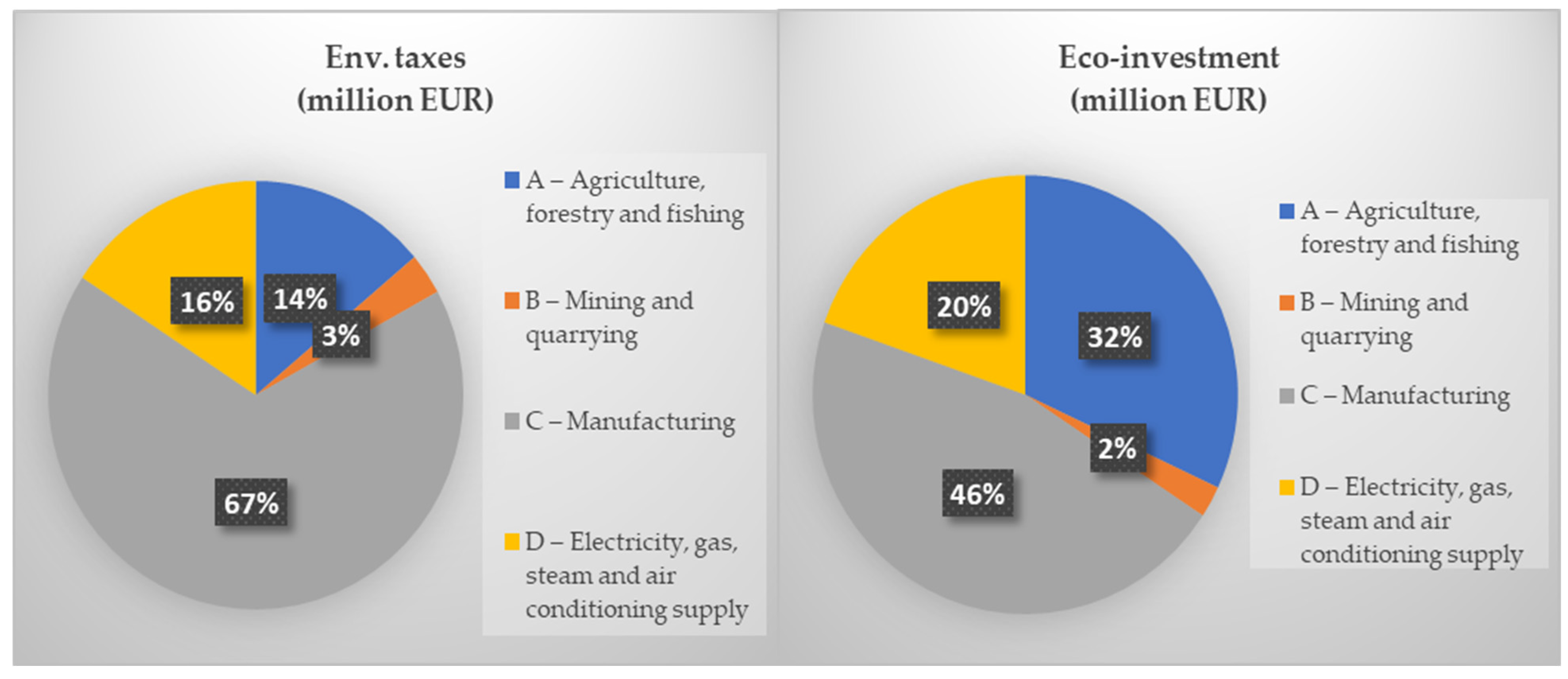
Source: Author’s calculations based on Eurostat data. EU-27 excluded to avoid double-counting.

reveals a clearly pronounced asymmetry between the distribution of environmental taxes and eco-investments. Manufacturing (sector C) generates 67.3% of total environmental taxes but accounts for 46.1% of eco-investments. Conversely, the agriculture sector (A) contributes 13.9% of tax revenues but constitutes 32.0% of investments, while also recording the highest investment intensity (2.71% of GVA). This configuration admits the interpretation that the distribution of investments does not directly follow the distribution of the tax burden. One possible reason is the role of targeted subsidies, particularly within the Common Agricultural Policy, which may channel investments towards certain sectors. This hypothesis, however, cannot be tested directly with the available data.

The energy sector (D) stands out with the highest tax intensity (6.61% of GVA), which is consistent with its exposure to energy taxation and emissions trading mechanisms. Its investment intensity of 1.57% of GVA, although moderate, may underestimate total environmental capital expenditure if compliance costs under the EU Emissions Trading Scheme (EU ETS) are not fully reflected in the investment data. This hypothesis cannot be verified in the present analysis due to the lack of sectoral data on ETS exposure.

Figure 4 presents the sectoral structure of the two indicators for the seven national economies for the period 2014–2023. A clearly pronounced asymmetry is observed between the distribution of environmental taxes and eco-investments. Manufacturing (sector C) generates 67.3% of environmental taxes but accounts for 46.1% of eco-investments. Conversely, agriculture (sector A) forms 13.9% of tax revenues but constitutes 32.0% of investments. This configuration shows that the distribution of investments does not coincide with the distribution of the tax burden. One possible interpretation is the role of targeted policies, including instruments within the Common Agricultural Policy, which may channel investments towards certain sectors. This hypothesis, however, cannot be verified directly with the available data.

The observed imbalance calls into question the assumption of a direct proportional relationship between tax burden and investment response. If such a relationship were present, it would be expected that sectors with higher tax payments would also realise higher investments. In the case of manufacturing, however, a different pattern is observed. This descriptive result does not provide evidence of a causal relationship, but substantiates the need for subsequent formal testing within the regression analysis.

Table 10. Heatmaps of average environmental tax burden and eco-investment intensity by country and sector (% of GVA, 2014–2023).

(a) Avg. Environmental Tax Burden (% of GVA, 2014–2023)					(b) Avg. Eco-Investment Intensity (% of GVA, 2014–2023)
Country	Agriculture (A)	Mining (B)	Manufacturing (C)	Electricity (D)	Country	Agriculture (A)	Mining (B)	Manufacturing (C)	Electricity (D)
BE	4.59%	4.98%	1.88%	6.14%	BE	9.71%	0.00%	0.56%	0.00%
BG	2.88%	2.23%	1.69%	14.77%	BG	1.27%	0.45%	1.08%	2.01%
FR	2.79%	6.72%	1.32%	0.53%	FR	4.68%	0.84%	0.90%	1.44%
HU	3.24%	3.49%	1.76%	2.11%	HU	1.47%	0.27%	0.20%	0.38%
IT	3.59%	8.74%	2.24%	6.41%	IT	0.24%	1.15%	0.18%	1.56%
PL	3.63%	1.26%	2.88%	1.71%	PL	1.18%	0.45%	0.35%	4.05%
RO	0.54%	4.08%	4.75%	14.62%	RO	0.40%	4.26%	0.18%	1.53%
Average	3.04%	4.50%	2.36%	6.61%	Average	2.14%	1.06%	0.49%	1.57%

Source: Author’s calculations.

offers a cross-tabulated presentation of the two key intensity indicators. Panel (a) shows that the energy sector of Bulgaria bears the highest mean tax burden (14.77% of GVA), closely followed by the energy sector of Romania (14.62%) and the mining industry of Italy (8.74%). Panel (b) shows that the agriculture sector of Belgium registers the highest investment intensity (9.71% of GVA), followed by the agriculture sector of France (4.68%) and the mining industry of Romania (4.26%). Notably, a number of country–sector pairs with a high tax burden do not show correspondingly high investment intensity (e.g., the energy sector of Romania: 14.62% taxes versus 1.53% investments; the energy sector of Bulgaria: 14.77% taxes versus 2.01% investments). This further underscores the need for a multifactor analysis that controls for unobserved heterogeneity across countries and sectors.

The descriptive analysis outlines three key preliminary conclusions. First, eco-investments and environmental taxes differ drastically across individual countries and sectors. There is no typical behaviour—Belgium and France invest increasingly more, while Romania and Italy contract. This diversity means that answers cannot be sought through simple averages—a panel approach is needed that accounts for what is specific to each country and sector. Second, taxes and investments move in different directions. Environmental taxes rise in most countries, but eco-investments decline in five out of seven. The divergence between the two trends does not establish a causal relationship, but calls into question the assumption of an automatic stimulating effect and motivates further econometric analysis. Third, the sectoral picture tells its own story. Manufacturing pays the most taxes (67% of the total) but does not invest proportionally more. Agriculture shows the reverse pattern—high investment intensity with a low tax burden, which is compatible with the hypothesis of the role of targeted subsidies under the CAP, although this cannot be tested with the available data.

4.3. Correlation Analysis

Before proceeding to the regression analysis, an examination is conducted of whether a statistical relationship exists between environmental taxes and eco-investments—and to what extent it is real, as opposed to being explained by the influence of the size of the economy.

At first glance, the relationship appears very strong.

Table 11. Pearson correlation matrices: (a) absolute values (million euro); (b) intensity ratios (% of GVA).

(a) Absolute Values (Million Euro)							(b) Intensity Ratios (% of GVA)
	Eco-Investment	Eco-Expenditure	Env. Tax	GVA	GDP			Eco-Invest (% of GVA)	Env. Tax (% of GVA)
Eco-Investment	1.00	0.68	0.93	0.90	0.74		Eco-Invest (% of GVA)	1.000	0.079
Eco-Expenditure	0.68	1.00	0.61	0.58	0.66		Env. Tax (% of GVA)	0.079	1.000
Env. Tax	0.93	0.61	1.00	0.94	0.69
GVA	0.90	0.58	0.94	1.00	0.56
GDP	0.74	0.66	0.69	0.56	1.00

(a) shows that the correlation between eco-investments and environmental taxes in absolute terms is r = 0.926 (p < 0.001). This result, however, is statistically misleading. Both variables correlate strongly with GVA (r = 0.90 and r = 0.94) and GDP (r = 0.74 and r = 0.69). Larger economies simply have more of everything—more taxes, more investments, higher GVA. This does not mean that taxes stimulate investments—it means that both grow with the size of the economy.

What does the relationship look like when the influence of the size of the economy is removed? Table 11(b) shows the correlations between the relative indicators (% of GVA), which are already adjusted for the size of the sector. The result is surprising—the correlation between tax burden and investment intensity drops to r = 0.079 and is not statistically significant (p = 0.161). In other words, when the size of the economy is accounted for and the tax burden and investment activity are compared as shares of gross value added, the apparently strong relationship breaks down.

4.4. Panel Regression Analysis

The correlation analysis showed that the observed simple relationship between taxes and investments is to a considerable extent the result of the scale effect. But correlation does not control for unobserved country and sector specifics—such as regulatory traditions, technological structure, or the policy environment. For this reason, the analysis proceeds to fixed-effects (FE) panel regressions, which isolate the within variation; that is, they answer the question: when taxes change over time within the same sector and country, do investments change as well?

A balanced panel of 28 units (seven countries × four sectors) over 10 years (2014–2023) is used. All monetary values are in real prices (base 2015).

Table 12. Fixed-effects panel regressions: eco-investment as dependent variable.

	M1 FE log-log	M2 FE Intensity	M3 FE+TE lag	M4 FE int.lag	M5 FE + Controls	M6 FE+TE Full
ln(EnvTax)	0.016 (0.152) [0.914]
Tax int. (%VA)		1.192 (3.892) [0.760]
ln(EnvTaxt−1)			0.098 (0.129) [0.450]
Tax int.t−1				3.748 (3.924) [0.341]	0.051 (0.042) [0.232]
ln(Lag EnvTax)						0.286 (0.188) [0.129]
ln(VA)	−0.025 (0.348)		0.175 (0.390)			0.197 (0.443)
EcoExp int.					0.027 (0.141) [0.849]
ln(EcoExp)						−0.081 (0.162) [0.618]
VA growth (%)					−0.000 (0.000) [0.002]
R2 within	0.0001	0.0009	0.0058	0.0075	0.0340	0.0246
N	269	280	252	252	252	197
Entity FE	Yes	Yes	Yes	Yes	Yes	Yes
Time FE	No	No	Yes	No	No	Yes
F-test (p)	0.987	0.760	0.450	0.341	0.002	0.487

Source: Author’s calculations. All values in real 2015 prices. Clustered SE by entity. (SE), [p].

presents six model specifications: Model 1 examines the logarithmic relationship (elasticity), Model 2 uses relative indicators (% of GVA), Model 3 adds time effects and a lagged tax, and Model 4 combines intensity with a lag. Model 5 adds new control variables (eco-expenditures and GVA growth), and Model 6 presents the full specification with lagged tax, eco-expenditures, and time effects. All models use clustered standard errors by units, justified by the results of the tests for heteroscedasticity and serial correlation (Section 4.1).

The results from all six models are unambiguous—none finds a statistically significant effect of environmental taxes on eco-investments. In Model 1, the elasticity is 0.016 (p = 0.914)—practically zero. In Model 2, the coefficient of tax intensity is 1.19, but with an enormous standard error (3.89) and p = 0.760. Model 3 tests whether taxes operate with a delay—but the lagged value is also insignificant (p = 0.450). Model 4 repeats the same result for the intensities. In Model 5, which includes eco-expenditures and GVA growth as control variables, the lagged tax intensity remains insignificant (β = 0.051, p = 0.232). The only significant variable in this model is the growth of real GVA (p = 0.002), which shows that macroeconomic conditions matter for the dynamics of eco-investments, but tax pressure does not. Model 6 (full model with lagged tax, eco-expenditures, and time effects) shows the highest coefficient for lagged taxes (β = 0.286, p = 0.129)—marginal but still insignificant at the conventional 5% level. This result suggests a possible delayed effect that may become significant over a longer time horizon—a hypothesis for future research.

Particularly telling is the R² within—the indicator that measures how much of the within-unit variation the model explains. In the baseline models (1–4), it is below 1%. The extended models (5–6) raise it to 2.5–3.4%, but this remains very low. The low explanatory power means that environmental taxes explain a negligible share of the variation in eco-investments within units. This is not necessarily a problem of the model; rather, it reflects the fact that investment decisions are determined by factors not included in the model: access to financing, sectoral regulation, technological maturity, subsidies, and strategic priorities of firms (Dechezleprêtre & Sato, 2017).

The Hausman test (

Table 13. Hausman test: FE vs. RE.

Test	χ2	df	p-Value	Decision
Model 1: log-log	3.4181	2	0.181	RE acceptable (p > 0.05)
Model 2: intensity	-	1	1.000	RE acceptable (p > 0.05)

Source: Author’s calculations.

) does not reject the null hypothesis in either case (p = 0.181 and p = 1.000), which shows that the RE model is acceptable. Nevertheless, FE remains the preferred model, since it is more conservative and does not require the additional assumption of independence between unit effects and regressors. The RE estimates are also insignificant for the tax variable (Model 1 RE: β = 0.07, p = 0.566; Model 2 RE: β = 3.32, p = 0.442).

To test whether the effect of taxes varies across sectors, a model with interaction effects (Tax intensity × Sector) is applied.

Table 14. Interaction model: Tax intensity × Sector.

	M7: Interactions Only	M8: Interactions + Controls
Tax × Agriculture (A)	−0.009 (0.054) [0.871]	−0.067 (0.067) [0.319]
Tax × Mining (B)	0.200 (0.133) [0.135]	0.161 (0.117) [0.169]
Tax × Manufacturing (C)	0.034 (0.045) [0.450]	0.027 (0.027) [0.311]
Tax × Electricity (D)	−0.004 (0.036) [0.903]	0.027 (0.027) [0.328]
EcoExp intensity		0.029 (0.140) [0.837]
VA growth (%)		−0.000 (0.000) [0.009]
R2 within	0.019	0.039
N	280	252
Entity FE	Yes	Yes
F-test robust (p)	0.582	0.020

Source: Author’s calculations. (SE), [p].

presents two variants: M7, with interaction effects only; and M8, with added control variables (eco-expenditures and GVA growth).

No sector shows a statistically significant tax effect at the conventional 5% level. Mining and quarrying (NACE B) is closest to significance (β = 0.200, p = 0.135 in M7; β = 0.161, p = 0.169 in M8), which may reflect a stronger response in a sector with high energy intensity. In Model 8 (with controls), GVA growth is again the only significant variable (p = 0.009). The results show that the observed absence of a tax effect is not masked by sectoral heterogeneity—it is consistent across all four NACE sectors.

4.5. Granger Causality Test

The regression analysis found no significant relationship between taxes and investments. However, the question remains—might the relationship run in the opposite direction, with higher investments leading to higher taxes? The Granger test examines both directions—whether past values of one variable improve the forecast for the other, beyond its own lags.

The results are categorical (

Table 15. Panel Granger causality test.

Direction	Lags	F-Stat	p-Value	Result
Tax → Invest (log)	1	1.4259	0.234	Not signif.
Invest → Tax (log)	1	0.0767	0.782	Not signif.
Tax → Invest (log)	2	0.8882	0.413	Not signif.
Invest → Tax (log)	2	0.0548	0.947	Not signif.
Tax int. → Invest int. (%GVA)	1	1.6402	0.202	Not signif.
Invest int. → Tax int. (%GVA)	1	0.8992	0.344	Not signif.
Tax int. → Invest int. (%GVA)	2	0.2440	0.784	Not signif.
Invest int. → Tax int. (%GVA)	2	1.1540	0.318	Not signif.

Source: Author’s calculations. F-test for joint significance of X lags in FE model.

). None of the eight tests rejects the null hypothesis. Taxes do not predict investments (highest F = 1.64, p = 0.202), but neither do investments predict taxes (lowest p = 0.318). The result is the same with 1 and 2 lags and under both specifications (log-log and intensity). In other words, the two variables move independently of one another over time. It should be noted that with a short time horizon (T = 10), the Granger test has limited statistical power, particularly for detecting delayed effects beyond 2 lags. Consequently, the absence of significance cannot categorically exclude a causal relationship over a longer horizon.

4.6. Robustness Checks

The question remains, however, whether the absence of an effect is not due to the particularities of the chosen model or the composition of the sample. For this reason, the main model is repeated under nine alternative settings (

Table 16. Robustness checks: environmental tax coefficient across specifications.

Specification	β (EnvTax)	SE	p-Value	R2 Within	Diagnostic Concern
Baseline FE (intensity)	0.012	0.039	0.756	0.001	Reference
R1: Random Effects	0.033	0.025	0.179	0.007	Estimator dependence
R2: First differences (log)	−0.063	0.208	0.765	0.008	Non-stationarity
R3: Excl. 2020-21 (COVID-19)	0.028	0.158	0.858	0.002	Pandemic shocks
R4: New EU members only	0.066	0.126	0.601	0.003	Sample heterogeneity
R5: Old EU members only	−0.094	0.320	0.770	0.010	Sample heterogeneity
R6: Intensity + time FE	0.016	0.038	0.669	0.001	Common time shocks
R7: Alt. DV (eco-expend.)	−0.005	0.016	0.774	0.000	DV specificity
R8: Winsorised 1%/99%	0.029	0.061	0.638	0.003	Outlier influence

Source: Author’s calculations. All models use real 2015 prices and clustered SE. Column ‘Diagnostic concern’ indicates what each check addresses.

). Each check addresses a specific diagnostic concern.

The result is consistent—all nine checks confirm the insignificance of the tax coefficient. No specification yields p < 0.05. The closest to significance is R1 (random effects: p = 0.179). Changing the sample, excluding the COVID-19 years, switching to first differences, replacing the dependent variable, Winsorising extreme values, and adding time effects—nothing alters the main conclusion.

Each check addresses a specific diagnostic concern. R1 tests whether the result depends on the estimation method—it does not. R2 eliminates potential non-stationarities—the result is preserved. R3 controls for pandemic disruptions—no change. R4–R5 test whether there is a difference between old and new EU member states—in both sub-samples the tax effect is insignificant, although the coefficient is slightly positive for new members and slightly negative for old members. R6 absorbs common time shocks (e.g., EU-wide policy changes)—no change. R7 replaces the dependent variable with eco-expenditures—the effect remains null, which shows that the result is not specific to capital investments. R8 controls for the influence of extreme values through Winsorisation—no change.

These checks strengthen the confidence that the null result is not accidental. Within this panel, there is no econometrically confirmed direct relationship between environmental taxes and eco-investments—in either direction. This result is robust to deflation, changes in model specification, the composition of the sample, treatment of extreme values, and choice of dependent variable.

5. Discussion

The present discussion interprets the results in the context of the three formulated hypotheses and compares them with the available literature. The main conclusion is that within the sample under consideration no robust direct relationship is established between environmental taxes and sectoral eco-investments, and therefore H1 is not confirmed. No statistically significant sectoral variation in this effect is found either, which does not support H2. Partial support is received for H3, insofar as macroeconomic dynamics—measured by real GVA growth—is the only variable that shows a persistent statistically significant effect in the extended specifications. These results hold under alternative specifications, sub-samples, deflation and robustness checks.

A substantial result of the study is the stark divergence between the correlations calculated with absolute values and those based on relative magnitudes. The correlation between the absolute values of environmental taxes and eco-investments is exceptionally high (r = 0.926), but it primarily reflects the scale of the economy—larger economies pay more taxes and make more investments, but not necessarily do so because of a causal relationship between the two variables. When the influence of scale is eliminated through relative magnitudes (taxes and investments as a percentage of GVA), the correlation drops to r = 0.079 (p = 0.161)—statistically insignificant and practically zero.

This result has direct relevance for financial analysis and risk management. Many existing policy analyses and ESG assessments operate with absolute values, which creates a risk of systematic error in evaluating policy effectiveness and in the pricing of transition risk. This problem is analogous to the well-known statistical phenomenon of spurious correlation, when two variables correlate strongly only because both are a function of a third variable—in this case the scale of the economy. For investment portfolios and ESG ratings that incorporate indicators of environmental taxation, this result means that absolute values are not a reliable indicator of policy effectiveness, especially in the presence of discrepancies in methodologies and measurement across different evaluators (Chatterji et al., 2016; Berg et al., 2022).

The central result of the study—the absence of a statistically significant direct relationship between environmental taxes and eco-investments in the sample under consideration (β = 0.016, p = 0.914, R² within < 1%)—is not isolated in the literature but adds an important new dimension. It should be emphasised, however, that this result shows what is observable within the specific panel, with the specific variables and specifications. It does not mean that environmental taxes cannot in principle stimulate eco-investments; rather, that in this sample the direct relationship is not statistically detectable. Morley (2012) establishes an effect on emissions but not on energy consumption, which suggests that taxes can reduce pollution without stimulating capital investments. Liobikienė et al. (2019), analysing 28 EU member states for the period 1995–2012, do not establish a statistically significant direct or indirect (through energy intensity, fossil energy consumption and renewable energy) effect of energy taxes on greenhouse gas emissions in the panel analysis. Our study confirms this conclusion but extends it in a new direction—the absence of effect pertains not only to emissions but also to capital eco-investments at the sectoral level.

Particularly indicative is the comparison with Carfora et al. (2021), who establish that the environmental tax burden constitutes a barrier to investments in renewable energy sources in the EU. Our result is compatible with the interpretation that environmental taxes can operate through two opposing channels. On the one hand, they raise the price of pollution and create an incentive for adaptation. On the other, they can constrain the available resource for investments, especially in sectors with high tax exposure and limited financial flexibility. Under such a configuration, the net effect can be weak or statistically undetectable.

At the same time, our result contrasts with the positive findings of Andersson (2019) and Sen and Vollebergh (2018). This, however, is not a contradiction but a difference in the object of analysis. These studies measure the effect on emissions, which is a more immediate channel (through consumption reduction), whereas we measure the effect on capital investments—a longer-term and indirect channel that requires a stronger and more sustained price signal. As Dechezleprêtre and Sato (2017) point out, even when regulations stimulate innovation, the benefits are often insufficient to compensate for the costs borne by regulated enterprises. This distinction is methodologically important—a null result for investments does not necessarily mean a null effect for emissions. Taxes may reduce pollution through behavioural change (lower consumption) without generating capital investments in cleaner technologies.

An important limitation in the interpretation is that the main independent variable (tax revenue) is an imperfect proxy for the tax intensity of the stimulus facing firms. As noted in the methodology, a change in tax revenue can stem from a change in the tax rate (the actual signal) but also from changes in output volume, price effects or changes in the tax base. The use of relative indicators (% of GVA) eliminates the scale effect but does not distinguish the remaining components. Consequently, interpreting the regression coefficient as a parameter of investment response to tax policy is ambitious and should be considered with the necessary caution (Köppl & Schratzenstaller, 2023). More broadly, in the absence of instrumental variables or a quasi-experimental design, the observed relationships in the present study should be interpreted as associative rather than causal. Endogeneity remains an unresolved structural problem, since tax revenues can simultaneously be a predictor and a result of investment behaviour, and omitted variables can shift the estimates in an unknown direction. Furthermore, it is possible that successful environmental policy reduces the tax base itself, which would weaken the observable relationship between taxes and investments. In the present study, however, the Granger test does not provide evidence of a predictive relationship in the reverse direction, although this result should be interpreted cautiously given the limited time horizon.

The descriptive analysis reveals a substantial sectoral imbalance—manufacturing (NACE C) pays 67% of environmental taxes but represents only 46% of eco-investments. Agriculture (NACE A) pays 14% but receives 32% of investments. This asymmetry is compatible with the hypothesis that the distribution of investments is determined more by access to targeted subsidies (e.g., under the CAP) and the sectoral regulatory environment than by the tax burden. It should be noted that this hypothesis is not directly tested in the model due to the lack of sectoral data on subsidies (Eurostat’s ESST data are voluntary and incomplete for the analysed period). This pattern raises questions about the correspondence between the polluter pays principle and the actual distribution of investments in the context of the Task Force on Climate-related Financial Disclosures (TCFD, 2017)—revenues are generated in some sectors, while investments are channelled towards others.

This result is compatible with the findings of Marin and Vona (2021), who emphasise that the impact of energy prices depends critically on sectoral specifics. The model with interaction effects (Tax × Sector) confirms that no sector shows a statistically significant tax effect (p > 0.05 in all four sectors). Mining (NACE B) is closest to significance (β = 0.200, p = 0.135), which may merit more in-depth investigation with a longer panel. The energy sector (NACE D) in our data has the highest tax intensity but comparatively low investment activity—a pattern compatible with the hypothesis of a “tax trap”, a sector with a high tax burden and a low investment response. This hypothesis, however, cannot be confirmed with descriptive data alone and requires additional modelling. Regardless, this mechanism is of key importance for assessing the financial risk of enterprises in the regulated sectors.

The extended models add several important nuances. First, real GVA growth is the only variable that shows a statistically significant effect on eco-investments across multiple specifications (p = 0.002 in Model 5; p = 0.009 in Model 8 with interactions). This suggests that the investment decisions of enterprises are more sensitive to macroeconomic conditions than to tax pressure. Second, the full model with a lagged tax (Model 6: β = 0.286, p = 0.129) shows the highest coefficient for the tax variable—borderline but still insignificant. This result admits the interpretation that the tax effect may manifest with a longer delay than the panel permits to capture (T = 10).

The Granger test does not find causality in either direction—taxes do not predict investments nor the reverse (all eight specifications with p > 0.05). This result means that the two variables move independently over time. It should be noted, however, that with T = 10 the test has limited statistical power, especially for delayed effects beyond two lags. Consequently, the absence of Granger causality cannot categorically rule out a causal relationship over a longer horizon. If taxes do not generate an investment response within 1–2 years, this is compatible with the interpretation that they function more as a fiscal instrument than as a stimulus for capital investments—at least in the short and medium term.

This observation corresponds with the theoretical model of Acemoglu et al. (2012), which shows that optimal policy requires a combination of carbon taxes and research subsidies, not taxes alone. Our empirical data support this position—taxation on its own is insufficient for generating environmental investments at the sectoral level. A holistic approach is needed that combines fiscal and non-fiscal instruments (subsidies, regulatory standards, mandatory ESG disclosure) for the effective management of financial transition risk. Consequently, the null result should be interpreted as an argument against the assumption of a simple, direct transmission mechanism from taxes to investments, rather than as an argument against the broader effectiveness of environmental policy packages in which taxation is only one of the complementary instruments.

The null result is not accidental. The nine robustness checks—random effects, first differences, exclusion of the COVID-19 years, separation of old and new EU member states, relative indicators with time fixed effects, an alternative dependent variable (eco-expenditure) and the Winsorising of extreme values—all confirm insignificance (p > 0.05 in all specifications). The closest to significance is the random-effects model (p = 0.179), followed by the sub-sample of new member states. The latter may reflect a stronger marginal effect in economies where eco-investments are only beginning to gain momentum—a hypothesis that merits future investigation.

6. Conclusions

The present study analyses the relationship between environmental taxes and eco-investments at the country–sector level in seven EU member states and four sectors according to NACE Rev. 2 for the period 2014–2023. The monetary indicators are deflated in real prices with a base year of 2015, and the empirical analysis is built upon a consistent multi-step strategy comprising diagnostic tests, descriptive and correlation analysis, panel regressions, Granger test and robustness checks. The main result is clear—within the sample under consideration no robust direct relationship is established between environmental taxes and capital eco-investments.

This conclusion should be interpreted within the specific scope of the data used. The dependent variable covers sectoral investments in environmental protection measured according to EPEA, and not all green investments or investments related to the climate transition in a broader sense. Therefore, the results pertain precisely to this category and should not be generalised automatically beyond it. The results obtained also show that the strong correlation in absolute values largely reflects the scale of the economy and weakens when relative indicators are used. The panel regressions with fixed effects do not establish a significant tax effect in any specification, and the only persistently significant predictor is real GVA growth. The Granger test also does not find causality in either direction. The descriptive analysis reveals a distinct sectoral imbalance as well: manufacturing generates a larger share of environmental taxes than of eco-investments, while in agriculture the reverse picture is observed, probably linked to the role of targeted instruments such as the CAP.

From a practical standpoint, the results point to several important conclusions:

• The mere presence of a tax does not guarantee an investment response. A more effective approach is to have a predictable mechanism whereby part of the revenue is returned to the sectors that generate them—for example through the co-financing of eco-projects. This improves the predictability of financial flows and reduces investment uncertainty for enterprises.
• A uniform tax approach does not account for the fact that sectors differ in technological structure and investment capacity. Therefore, sectoral differentiation and/or combining the tax with targeted instruments is justified where tax intensity is high but the investment response is weak (for example in the energy sector).
• The absence of a direct effect supports the thesis that environmental taxes probably operate more effectively as part of a broader policy package than as an independent stimulus. This points to the need for a coordinated combination of tax, regulatory and financial instruments tailored to sectoral specificities.
• The results also show the importance of using relative rather than only absolute indicators when assessing policy effectiveness, since the scale of the economy can create a misleading impression of the strength of the relationship between taxation and investments. This is relevant both for the public assessment of policies and for financial analysis and the management of ESG risks.

The study also has several limitations that outline directions for future work. The sample is limited to seven countries, four aggregated sectors and a comparatively short time horizon, which does not permit reliable testing of longer lags or the use of dynamic panel models. Furthermore, tax revenue remains an incomplete measure of the real tax and regulatory pressure, and the model does not include certain potentially important factors such as environmental subsidies, energy prices by sector, exposure to the EU ETS and access to green finance. Additionally, the dependent variable used covers only investments in environmental protection according to EPEA and does not include other forms of green investments such as resource efficiency, energy efficiency, renewable energy sources or climate adaptation. Nevertheless, the fact that the absence of a statistically significant effect holds across different model specifications shows that the result can hardly be explained solely by a peculiarity of one specific model. Future studies can extend the time horizon, include more direct measures of the tax and regulatory stimulus and trace the possible indirect channels of impact, for example through current eco-expenditure, technological changes or changes in energy intensity.

The present study does not deny the role of environmental taxes as a price signal and an instrument for limiting pollution. In the countries and sectors under consideration, however, the expectation that higher environmental taxes are associated with higher sectoral eco-investments is not confirmed. This shows that the effect of policy instruments should be assessed on the basis of real data rather than prior expectations. Consequently, the result should not be interpreted as a rejection of the effectiveness of environmental policy as a whole, but as an argument against the assumption of a simple and direct mechanism of impact between environmental taxes and eco-investments.