Optimal and Non-Optimal MACD Parameter Ranges with Stop-Loss and Take-Profit Rules: Evidence from the Gold Market

Abstract

This study investigates optimal and non-optimal MACD parameter ranges in the gold market using a simulation-based framework and examines their implications for trading strategy design and risk-adjusted performance. By systematically identifying optimal and non-optimal MACD parameter ranges together with appropriate stop-loss and take-profit levels, this study addresses an issue that has not been explored in the existing literature on gold markets. The empirical results reveal a clear contrast between the optimal and non-optimal groups. Importantly, the superior performance of the optimal strategies emerges at the group level, rather than being driven by isolated exceptional models. Annual analysis further shows that models in the optimal groups respond effectively to overall market direction, taking long (short) positions under upward- (downward-) biased market conditions. Additional analyses examine fixed-ratio stop-loss and take-profit rules, identifying parameter–strategy combinations that balance risk control and profit realization. A cross-market comparison between the gold and stock markets highlights significant heterogeneity in optimal parameter ranges and investment horizons, underscoring the market-specific nature of MACD-based trading rules and the limits of cross-asset parameter transferability. Overall, these findings provide deeper insights into market-specific trading dynamics, going beyond the provision of an empirical benchmark and a methodological reference for MACD-based trading strategy design in the gold market.

1. Introduction

Gold is widely recognized as a safe-haven asset, particularly during periods of political, economic, or geopolitical instability. As a tangible asset, gold is largely free from credit risk and direct government intervention, and its price movements tend to exhibit low or even negative correlations with equities and major currencies. These characteristics make gold an effective instrument for portfolio diversification, helping to offset potential losses in other asset classes and improve risk-adjusted returns.

However, regardless of whether gold is employed as a risk-hedging instrument or for pursuing investment returns, effective trading decisions require careful consideration of evolving market dynamics, as in equity markets. In this context, the Moving Average Convergence Divergence (MACD)—one of the most widely used technical indicators—is applied in gold markets to generate trade signals.

The MACD is defined by three parameters and is typically expressed in the form MACD (n₁, n₂, n₃), such as MACD (12, 26, 9). The first two parameters determine the MACD line, which is calculated as the difference between the short-term (n₁) and long-term (n₂) exponential moving averages of historical prices. The third parameter defines the signal line, which is the exponential moving average of the MACD line over n₃ periods. Trading signals are generated at the points where the two lines cross. A crossover of the MACD line above the signal line indicates a potential buy signal, whereas a crossover below indicates a potential sell signal. This rule is commonly referred to as the “signal line crossover.”

However, like any technical analysis tool, the MACD indicator can generate false trading signals because its signals depend critically on the choice of the three parameters. Consequently, it is essential to adjust the parameter values to align them with both the investment objective and the characteristics of the market under study.

For reference, the commonly used (12, 26, 9) parameter setting is neither a formal standard nor Appel’s (1979) original recommendation. Appel, who developed the MACD, suggested (8, 17, 9) for buy signals and (12, 25, 9) for sell signals.1 Nevertheless, over the past two decades, many studies have adopted the (12, 26, 9) setting as a default configuration, either to evaluate the indicator’s effectiveness or to assess market efficiency. Before turning to the main focus of this study, it is therefore useful to briefly review this line of research.

Several studies have reported weak or negative performance of the MACD (12, 26, 9) model across different equity markets. Meissner et al. (2001) found that the MACD performed poorly for constituent stocks of the Dow Jones Industrial Average and the NASDAQ-100, describing it as “almost a contra-indicator.” Armour et al. (2010) reported that the MACD (12, 26, 9) model failed to outperform buy-and-hold strategies in the Irish stock market. Similar results for the Spanish stock market were reported by Rosillo et al. (2013). Biondo et al. (2013) examined the MACD (12, 26, 9) model together with other conventional technical trading strategies, noting that “the standard trading strategies they considered were riskier than the random strategy.”

A related strand of the literature links MACD performance to market efficiency. Chen and Metghalchi (2012) evaluated 32 variations of single-, double-, and triple-indicator combinations constructed from six widely used technical indicators on the Brazilian stock index (BOVESPA). None of these models—including the MACD (12, 26, 9)—outperformed a buy-and-hold strategy, leading them to conclude that “our results strongly support the weak-form of market efficiency of the Brazilian stock market.” Nor and Wickremasinghe (2014) similarly examined the performance of the MACD (12, 26, 9) model on the Australian All Ordinaries Index (XOA). They reported that, while the traditional MACD model generally yielded poor results, the Relative Strength Index (RSI) model exhibited some profit potential, and concluded that “overall, the Australian stock market is not weak-form efficient.”

Taken together, although the number of studies cited above is limited, most have failed to demonstrate profitable outcomes using the MACD with the traditional parameter setting. This raises the question of why the traditional setting should be regarded as the sole yardstick for assessing both the profitability of the MACD and the validity of market efficiency tests. Had alternative parameter values been explored, the resulting conclusions might have differed.

In this context, some prior research has documented positive evidence, although such cases are rare. A notable example is Chong and Ng (2008), who applied the MACD and RSI to the FT30 index and showed that these rules outperformed a buy-and-hold strategy. Interestingly, Chong et al. (2014), as a follow-up to this study, reported different results. They re-examined the MACD and RSI across five OECD stock markets and tested three standard MACD models—(12, 26, 0), (12, 26, 9), and (8, 17, 9)—with mixed outcomes. Specifically, the MACD (12, 26, 0) outperformed a buy-and-hold strategy in Italy, whereas the MACD (12, 26, 9) did not, and the MACD (8, 17, 9) produced significantly negative returns in Italy. Upon closer inspection of these contrasting results within the same market, it becomes clear that the profitability of the MACD models depends critically on parameter settings.

This issue becomes even more evident when considering the findings of Abbey and Doukas (2012), who investigated whether technical analysis—including the MACD (12, 24, 0) and three other well-known indicators—generated profitable outcomes for 428 individual currency traders. Their results showed that technical analysis was negatively associated with trader performance, which they attributed to traders’ reliance on well-known technical indicators. This finding can be interpreted as a pointed critique of the common practice of relying on popular indicators and their standard parameter settings simply because they are widely used, without careful scrutiny.

More recently, Montgomery et al. (2019) revisited this line of research by testing three MACD models on 50 U.S. corporate bonds and their corresponding stocks. All three models employed the traditional 12 and 26 settings and, consistent with earlier studies, were found to be unprofitable.

Within this context, only a few studies have explored the selection of appropriate MACD parameter values. Erić et al. (2009) tested MACD models with different settings to identify the most profitable parameters for companies listed on the Belgrade Stock Exchange. They noted that optimized parameter values for individual companies can substantially improve profitability. However, the parameters that performed best in in-sample tests all produced losses in out-of-sample tests, leading them to conclude that “it is important to optimize the three parameters over time.” Similarly, Borowski and Pruchnicka-Grabias (2019) examined optimal MACD parameters for companies on the Warsaw Stock Exchange. They reported that while a few companies shared identical optimal parameters, most differed, and that the highest performance was achieved with “odd-even-odd” combinations of the three parameters. Although the practical usefulness of this finding for market participants remains uncertain, this appears to be the first study to characterize optimal parameter combinations at the market level.

Against this backdrop, Kang (2021) demonstrated that applying the MACD (12, 26, 9) model to Japan’s Nikkei 225 futures index yielded deeply negative returns over the 2011–2019 period. In contrast, he showed that the MACD could generate substantial gains when its parameters were optimized. He further examined whether adding supplementary strategies to filter out false trading signals could enhance profitability. The findings indicated that these strategies were effective only when paired with optimized parameters, and that applying them to the traditional MACD model resulted in predominantly negative returns.

Building on this line of research, Kang (2023) proposed a methodology to identify optimal and non-optimal MACD parameter values for a given market and applied it to three major stock market index futures: the Nikkei 225, Dow Jones 30, and Nasdaq 100. The analysis identified market-specific ranges of optimal and non-optimal values for each of the three MACD parameters. Sample models constructed using the optimal parameter ranges generally generated significantly higher returns, outperforming both a buy-and-hold strategy and a random strategy, suggesting that these markets may not be weak-form efficient. More importantly, although the optimal parameter ranges differed across the three indices, the optimal combinations for each shared a distinctive structural pattern. This cross-market evidence highlights the presence of market-specific features in MACD parameter optimization.

However, since Kang (2023) primarily focused on stock markets, it remains unclear whether the same methodology can be applied to commodity markets such as gold. Identifying optimal and non-optimal parameter ranges in the gold market would not only help clarify the applicability of this parameter-optimization approach beyond equity markets, but also provide alternative insights into trading strategy design and gold market dynamics. In this context, a cross-market comparison between stock and gold markets is meaningful in terms of trading behavior and price dynamics because these two markets differ fundamentally in their volatility structures, trading characteristics, and investor profiles, which may give rise to distinct MACD parameter behaviors and associated investment horizons. Accordingly, this study examines the following research questions:

• What are the optimal and non-optimal MACD parameter ranges in the gold market, and how do they differ from those identified in stock markets by Kang (2023)? This question enables a cross-market comparison of optimal and non-optimal parameter ranges between gold and stock markets.
• How robust is the performance of the MACD system when implemented with the identified optimal parameter values? This question examines whether models based on these parameters maintain their effectiveness under varying market conditions, such as momentum shifts or structural changes.
• Could the MACD, when implemented with the identified optimal parameter values, deliver performance in the gold market that is distinct from that in stock markets? This question examines whether MACD-based strategies in gold can contribute to portfolio diversification, thereby offering potential benefits when combined with equity investments.
• Could the MACD models with the identified optimal parameter values retain their performance when stop-loss and take-profit rules are applied? This question examines how such exit rules—while limiting losses—may influence overall performance by potentially constraining upside gains.

The systematic investigation of these four questions forms the primary objective of this study. While extensive research has examined MACD-based trading strategies, no prior study has conducted an empirical analysis of MACD to identify both optimal and non-optimal parameter ranges together with appropriate stop-loss and take-profit levels. These issues have remained largely unaddressed, particularly in the context of the gold market. By addressing these gaps, this study provides a transparent empirical framework for evaluating MACD-based trading strategies in the gold market.

Given the growing use of machine learning (ML) and artificial intelligence (AI) methods in financial market prediction, it is important to clarify the methodological positioning of the present study. While such approaches often achieve strong predictive performance, they typically offer limited transparency and rarely emphasize the identification of interpretable MACD parameter values. Accordingly, this study adopts a conventional trading simulation framework, which allows for transparent evaluation of a large number of MACD parameter sets and facilitates the identification of both optimal and non-optimal parameter ranges, as well as appropriate stop-loss and take-profit levels.

2. Literature Review

This section reviews prior studies on gold market forecasting by outlining the main methodological approaches and their limitations, and by briefly discussing the determination of stop-loss and take-profit levels.

2.1. Methods for Forecasting Gold Market Prices and Trends

Gold market forecasting methods can be broadly classified into two categories: classical and modern approaches. Classical approaches typically include: (1) time-series and econometric models and (2) technical analysis. Modern approaches encompass (3) machine learning techniques, including deep learning models, and (4) hybrid frameworks that combine elements from multiple methodologies.

(1)

Time-series and Econometric Models

Time-series models analyze historical price data to capture temporal dependencies and trends, with ARIMA (Autoregressive Integrated Moving Average) and VAR (Vector Autoregression) models serving as representative examples. Classical econometric models, in particular, emphasize volatility dynamics and long-run relationships. GARCH (Generalized Autoregressive Conditional Heteroskedasticity) models are widely used to capture time-varying variance, while VECMs (Vector Error Correction Models) account for long-run equilibrium relationships among integrated time series.

Representative studies include Hassani et al. (2015), who applied VAR and ARIMA models to forecast monthly gold prices and found that these models struggled to outperform a random walk. By contrast, Gangopadhyay et al. (2016) reported that the VECM outperformed a random walk for Indian gold prices. More recently, Yousaf et al. (2021) examined gold’s role as a safe haven and hedge against thirteen Asian stock markets during the COVID-19 outbreak, employing dynamic conditional correlation (DCC)-GARCH models.

(2)

Technical Analysis Models

Technical analysis models rely on technical indicators—predefined mathematical functions applied to market data—to identify price trends and potential turning points. Commonly used indicators include the MACD, RSI, Moving Average (MA), and Bollinger Bands (BB). Among these indicators, the MACD is one of the most widely adopted across asset markets, owing to its intuitive structure and ease of implementation.

More broadly, technical trading rules have been shown to be frequently profitable under certain market conditions. For example, Lento and Gradojevic (2022) found that rules such as the MA and BB generated positive returns during the COVID-19 market crash across five asset markets, including Bitcoin, oil, and gold. However, systematic empirical evidence on the performance of the MACD in the gold market remains unexplored. Addressing this gap, the present study systematically examines both optimal and non-optimal MACD parameter ranges and their implications for trading strategy design in the gold market.

(3)

Machine Learning and Deep Learning Models

Traditional statistical models, such as ARIMA and GARCH, as well as technical analysis indicators, often struggle to capture complex and nonlinear market dynamics, motivating the use of more data-driven approaches (Taneva-Angelova et al., 2025). Consequently, machine learning (ML) and deep learning (DL) models have been increasingly applied to financial market forecasting.

ML approaches include tree-based classifiers, such as decision trees, random forests, and gradient boosting methods. DL architectures encompass artificial neural networks (ANN), convolutional neural networks (CNN), recurrent neural networks (RNN), long short-term memory networks (LSTM), and gated recurrent units (GRU).

Among the numerous studies in this field, Sadorsky (2021) provides an illustrative example by employing tree-based ML classifiers to forecast the price direction of gold and silver exchange-traded funds. The study also used technical indicators, such as the MA, MACD, and RSI, as input features—market-derived variables used to predict price direction.

(4)

Hybrid Models

Hybrid models integrate two or more methods to leverage complementary strengths and mitigate individual weaknesses, often improving predictive accuracy. Various hybrid frameworks have been proposed in the literature; the following two examples illustrate representative approaches for gold price prediction.

Mousapour Mamoudan et al. (2023) proposed a hybrid neural network-based metaheuristic framework to filter erroneous signals generated by technical analysis indicators and enhance the prediction of global gold prices. Signals derived from the MA, MACD, and Ichimoku indicators were used as input features, with moth-flame optimization (MFO) applied for feature selection. A combined CNN and bidirectional GRU (BiGRU) model was then employed to distinguish false signals from valid ones, while the firefly algorithm (FA) optimized hyperparameters and reduced computational cost.

Another example is Taneva-Angelova et al. (2025), who proposed a hybrid framework for multivariate gold price prediction by integrating classical econometric models, traditional ML algorithms, modern DL methods, and their hybrids to capture complex temporal dynamics and cross-variable relationships.

2.2. Limitations and Research Gaps in Existing Approaches

ML and DL models offer notable strengths, such as flexibility in capturing nonlinear relationships and strong predictive performance when large datasets are available. However, as noted in the Introduction, they also have limitations, including the risk of overfitting, high computational costs, and limited interpretability compared with traditional econometric or technical analysis approaches. Hybrid models inherit these issues and introduce further complexity, which reduces transparency.

Another important limitation concerns how technical indicators—such as the MACD—are used within ML, DL, and hybrid frameworks. These approaches have largely treated technical indicators merely as sources of input features. As a result, advanced ML, DL, and hybrid algorithms—such as CNNs, RNNs, LSTMs, or NN–metaheuristic frameworks—are employed to filter noise from these inputs and map them to trading signals. Consequently, optimal MACD parameter values are rarely identified explicitly and instead remain embedded within the models’ internal mechanisms. This reflects a reversed research priority: most studies optimize predictive accuracy internally rather than directly optimizing MACD parameters.

Genetic algorithms (GAs) provide an alternative approach by explicitly searching for optimal parameter values through fitness-based optimization, rather than learning directly from data as in ML or DL models. Although relatively few studies adopt this approach, Agudelo Aguirre et al. (2020, 2021) reported different GA-optimized MACD parameter sets for the NASDAQ Composite Index in two separate studies, obtaining (6, 15, 3) for the 2013–2019 period and (7, 10, 15) for the shorter 2013–2017 period. However, GA-based optimization is often unstable and difficult to reproduce, as results depend on random initialization, the specification of fitness functions, and hyperparameter choices.

Overall, existing studies offer limited systematic analysis of MACD parameter settings, and comprehensive discussions of stable, market-specific optimal parameter ranges remain largely absent. To bridge this gap, the present study systematically evaluates a wide range of MACD parameter sets in the gold market, enabling the identification of both optimal and non-optimal values.

2.3. Approaches for Determining Stop-Loss and Profit-Target Levels

Many studies have examined the effects of implementing stop-loss and/or take-profit rules, which close a position once the price falls below (stop-loss) or rises above (take-profit) a predetermined level. These rules are commonly classified into two categories: (i) fixed rules, defined at constant price levels or as proportions of the entry price, and (ii) dynamic mechanisms, in which thresholds vary with market volatility.

Examples of fixed rules include Krishnan and Menon (2009, as cited in Vezeris et al., 2018), who applied a constant take-profit level of 20 pips in trading systems incorporating technical indicators, including the MACD, and Bolgün et al. (2010), who set take-profit and stop-loss levels at 3% and 2% of the entry price, respectively.

In contrast, examples of dynamic approaches include Klement (2013), who determined stop-loss widths based on the annual standard deviation of returns, and Kaminski and Lo (2014), who expressed stop-loss and re-entry thresholds as standard deviations from the mean across multiple time frequencies.

More recently, Vezeris et al. (2018) examined several take-profit and stop-loss strategies within a MACD-based system across multiple assets, including ATR (Average True Range)-based stop-loss rules in which a volatility-scaled multiplier determined how tightly stop-loss levels were set relative to price movements, while varying both the multiplier and the ATR period length.

Overall, existing studies account for market volatility when setting thresholds, but the measures and calculation methods differ substantially. In light of this variation, the present study adopts simple fixed-ratio exit rules following Bolgün et al. (2010). Take-profit and stop-loss levels are set at either 5% or 10% of the entry price, allowing direct comparison across thresholds. This addresses the study’s second objective: assessing whether such simple exit rules enhance profitability and identifying which levels perform best in the gold market.

Compared with dynamic mechanisms, fixed-ratio rules are simpler, requiring no additional volatility estimation or parameter tuning. Although they do not explicitly incorporate volatility, the thresholds respond naturally to price movements; for example, a 5% threshold may be reached quickly in high-volatility markets but more slowly under low volatility.

3. Research Methodology

As noted in the Introduction, this study examines the applicability of Kang’s methodology, originally developed for stock index markets, to the global gold trading market. To achieve this objective and to ensure comparability with the stock market analysis of Kang (2023), this study conducts the analysis in a standardized manner, using the same MACD parameter search space, trading rules, and test period.

3.1. Parameter Search Space and Baseline Sample Models

This study considers all combinations of MACD parameter values ranging from MACD (3, 5, 3) to MACD (20, 40, 40), with the three parameters (n₁, n₂, n₃) specified as n₁ = {3, …, 20}, n₂ = {5, …, 40}, and n₃ = {3, …, 40}, each incremented by one day. These ranges yield 24,624 (=18 × 36 × 38) models with unique parameter value combinations. Among them, 5168 irrational models—where the short-term parameter n₁ is greater than or equal to the long-term parameter n₂—are excluded. The remaining 19,456 models constitute the baseline sample used for analysis in this study.

3.2. Trading Rules and Exit Conditions

The trading rules can be summarized as follows: (1) When a buy (sell) signal is generated by a MACD signal line crossover, a buy (sell) order for one trading unit is executed at closing price of the next day. (2) Once a position is established, any subsequent identical signals are ignored. When the first opposite signal appears, the existing position is closed at the next day’s closing price. (3) Simultaneously, to implement the newly generated signal, a reverse sell (buy) order for one trading unit is executed at that closing price. In this manner, each opposite signal both closes the current position and opens the reverse position. (4) Consequently, only one position of one trading unit can be held at any time; trades are executed sequentially, and overlapping positions are not permitted.

Note that this trading rule alternates between long positions, which profit from price increases, and short positions, which profit from price decreases. Accordingly, the performance of all sample models is evaluated separately for long and short trades in the trading simulations. Transaction fees are not considered, following Kang (2023), to maintain consistency with the previous study and ensure comparability of results.

The return of each transaction is computed using gold price as the log difference between the selling and buying prices, that is,

$$r_t={\mathrm{l}\mathrm{n}(P}_{sell})-{\mathrm{l}\mathrm{n}(P}_{buy})$$

(1)

where P_buy and P_sell denote the closing prices on the days when the buy and sell transactions are executed, respectively. A positive log return $r_t$ for the t-th transaction indicates a profit, while a negative value indicates a loss, regardless of trade direction.

To calculate the Exponential Moving Average (EMA) used in constructing the MACD series, the following recursive formula is applied:

$${EMA}_t={\displaystyle \frac{2}{n+1}}(C_t-{EMA}_{t-1})+{EMA}_{t-1}$$

(2)

where n denotes the number of periods used for the EMA, and $C_t$ represents the closing price on day t. In addition, this study introduces stop-loss and take-profit rules to examine whether simple risk-management rules can enhance profitability in the gold market. The rules are defined as follows:

$$\mathrm{Stop}-\mathrm{loss}\mathrm{thresholds}=\left\{\begin{array}{c}{P}_t\le P_e\left(1-x\right) \mathrm{f}\mathrm{o}\mathrm{r} \mathrm{a} \mathrm{l}\mathrm{o}\mathrm{n}\mathrm{g} \mathrm{p}\mathrm{o}\mathrm{s}\mathrm{i}\mathrm{t}\mathrm{i}\mathrm{o}\mathrm{n} \\ P_t\ge P_e\left(1+x\right) \mathrm{f}\mathrm{o}\mathrm{r} \mathrm{a} \mathrm{s}\mathrm{h}\mathrm{o}\mathrm{r}\mathrm{t} \mathrm{p}\mathrm{o}\mathrm{s}\mathrm{i}\mathrm{t}\mathrm{i}\mathrm{o}\mathrm{n}\end{array}\right.$$

(3)

$$\mathrm{Take}-\mathrm{profit} \mathrm{thresholds}=\left\{\begin{array}{c}{P}_t\ge P_e\left(1+x\right) \mathrm{f}\mathrm{o}\mathrm{r} \mathrm{a} \mathrm{l}\mathrm{o}\mathrm{n}\mathrm{g} \mathrm{p}\mathrm{o}\mathrm{s}\mathrm{i}\mathrm{t}\mathrm{i}\mathrm{o}\mathrm{n} \\ P_t\le P_e\left(1-x\right) \mathrm{f}\mathrm{o}\mathrm{r} \mathrm{a} \mathrm{s}\mathrm{h}\mathrm{o}\mathrm{r}\mathrm{t} \mathrm{p}\mathrm{o}\mathrm{s}\mathrm{i}\mathrm{t}\mathrm{i}\mathrm{o}\mathrm{n}\end{array}\right.$$

(4)

where $P_t$ denotes the current price, $P_e$ denotes the entry price, and $x\in \{0.05,0.1\}$, corresponding to 5% and 10%, respectively. Under these rules, a position is closed when a profit of 5% or 10% relative to the entry price is reached (take-profit), or when a loss of 5% or 10% occurs (stop-loss). These rules are applied in four standardized combinations of stop-loss and take-profit levels: 5%/5%, 10%/10%, 10%/5%, and 5%/10%.

3.3. Data

This study uses daily XAU/USD closing prices (3 January 2011−31 December 2021) obtained from Investing.com, a widely used platform for financial market data. XAU/USD represents the spot price of gold quoted in US dollars and is traded in the foreign exchange (forex) market in a manner similar to other currency pairs. As XAU/USD is one of the most widely used benchmarks for internationally traded spot gold prices denominated in U.S. dollars, it provides a representative measure of global gold price movements over the sample period. To enable year-by-year comparability with Kang (2023)’s study on stock markets, the same 11-year period of data is employed.

The dataset is divided into two segments: the first nine years (2011–2019) are used for in-sample testing, while the last two years (2020–2021) constitute the out-of-sample period. In addition, the in-sample data are further subdivided into three equal-length sub-periods—2011–2013, 2014–2016, and 2017–2019—to evaluate model profitability separately within each segment and enhance robustness against sample-specific effects. This procedure follows Kang (2023), who adopted the method of Chong and Ng (2008) to mitigate data-snooping bias.

3.4. Methodology for Identifying Optimal and Non-Optimal Parameter Ranges

The methodology proposed by Kang (2023) can be redefined as following four steps.

• Step 1: Model Simulation and Performance Evaluation
  In this step, the profitability of 19,456 baseline sample models is simulated and evaluated using gold market data from 2011 to 2019. Based on their performance, the top 100 and bottom 100 models are identified and retained as target models for subsequent analysis.
• Step 2: Examining Parameter Distributions and Marking Optimal/Non-optimal Values
  For the top and bottom 100 ranked models, the frequency distributions of the three parameter values (n₁, n₂, n₃) are examined. Parameter values whose frequency ratios meet or exceed a specific threshold—referred to as the minimum cutoff point—are marked as optimal (based on the top-performing models) or non-optimal (based on the bottom-performing models), reflecting their association with relatively superior or inferior performance. In this study, the minimum cutoff point is set at 5%.
• Step 3: Identifying Parameter Ranges and Constructing New Sample Models
  For the parameter values marked in Step 2, attention is focused on those clustered around the most frequently observed values. Consecutive marked parameter values are grouped and treated as a single continuous parameter range. When multiple distinct groups are identified, they are labeled as Group A, Group B, and so forth. New sample models are then constructed by combining parameter values within these predefined optimal and non-optimal ranges.
• Step 4: Validating the Performance of the New Sample Models
  This step evaluates the performance of the newly constructed sample models. Although these models are built using parameter values drawn from the original top and bottom 100 models, most do not coincide with those original models; instead, they consist of new parameter value combinations formed exclusively from the predefined optimal or non-optimal parameter ranges. It is therefore necessary to examine whether these newly constructed models exhibit systematic performance differences. If models using parameter values within the predefined optimal parameter ranges consistently outperform, while those based on non-optimal ranges underperform in both the in-sample and the out-of-sample periods, the observed performance differences can be reasonably attributed to the parameter settings themselves. In this case, the predefined parameter ranges can be regarded as optimal or non-optimal, providing evidence that they represent as optimal or non-optimal parameter value ranges in the tested market.

3.5. Implementation of the Methodology Using Gold Market Data

This section describes how the methodology outlined in the previous section is applied to the gold market. It focuses on Steps 1–3: analyzing the distributions of the three parameters among the top- and bottom-performing models, identifying the resulting optimal and non-optimal parameter ranges, and constructing new sample models based on these ranges. Step 4, which evaluates the performance of these new models, is covered in Section 4, where the empirical results are presented.

3.5.1. Parameter Distributions in Top/Bottom Models

Figure 1 illustrates the observed frequencies of n₁, n₂, and n₃ among the top- and bottom-ranked models (blue for top, red for bottom), selected from the full set of 19,456 baseline models. These distributions reveal how parameter values differ between models with superior and inferior performance. As the sample size increases, the variability of the distribution decreases, while the overall shapes remain largely unchanged; no substantial structural differences emerge even when the analysis is extended to the top and bottom 1000 models. This consistency suggests that the distributions observed for the top and bottom 100 models reflect characteristic patterns rather than incidental outcomes, supporting reliable analysis at this sample size.

Focusing on the top and bottom 100 models (left side of Figure 1), the most frequently used parameter values—and their concentration ranges—differ notably between the two groups. This contrast is most pronounced for n₂ and n₃, while n₁ shows substantial overlap. Accordingly, model performance varies mainly with respect to n₂ and n₃. These distributional differences may reflect gold-specific market dynamics captured by the MACD parameters, which will be revisited in later sections.

3.5.2. Ranges of Optimal and Non-Optimal Parameter Values

After examining the frequency ratios of the three parameters in the top and bottom 100 models, values with ratios at or above the 5% cutoff are marked as noteworthy for their association with superior or inferior performance. These ratios correspond to the numerical values on the histogram bars in Figure 1. Based on these marked values, optimal and non-optimal parameter ranges are identified following the procedure described in Step 3 (Section 3.4). The resulting optimal parameter ranges are as follows:

• A_n1: {5, …, 9} for the first parameter n₁;
• A_n2: {19, …, 22}, B_n2: {33, …, 40} for the second parameter n₂;
• A_n3: {20, …, 28}, B_n3: {37, …, 40} for the third parameter n₃.

Here, the subscript n₁, n₂, n₃ in A_n1, A_n2, A_n3 indicate the corresponding parameters. Notably, among the top 100 ranked models, 93% had their n₁ values within range A_n1, while for n₂, 78% of models fell within either A_n2 (24%) or B_n2 (54%). Similarly, for n₃, 72% fell within either A_n3 (48%) or B_n3 (24%).

The non-optimal parameter ranges are as follows, identified in a manner similar to the optimal ranges:

• W_n1: {4, …, 11} for the first parameter n₁;
• W_n2: {7, 8}, X_n2: {24, 25} for the second parameter n₂;
• W_n3: {4, …, 8} for the third parameter n₃.

Among the bottom 100 ranked models, 66% had their n₁ values within range W_n1, 32% fell within either W_n2 (21%) or X_n2 (11%), and 55% had their n₃ values within W_n3.

3.5.3. Construction of the New Sample Models

Using the values within the predefined “optimal” parameter ranges described above, four combinations are constructed, each consisting of three parameter ranges corresponding to n₁, n₂, and n₃:

• A_n1–A_n2–A_n3 (180);
• A_n1–A_n2–B_n3 (80);
• A_n1–B_n2–A_n3 (360);
• A_n1–B_n2–B_n3 (160).

The numbers in parentheses indicate the number of models generated for each combination. The size of each parameter range is n(A_n1) = 5, n(A_n2) = 4, n(A_n3) = 9, n(B_n2) = 8, and n(B_n3) = 4. Accordingly, the numbers of unique sample models are 180 models (=5 × 4 × 9) for A_n1–A_n2–A_n3, 80 models (=5× 4 × 4) for A_n1–A_n2–B_n3, 360 models (=5 × 8 × 9) for A_n1–B_n2–A_n3, and 160 models (=5 × 8 × 4) for A_n1–B_n2–B_n3, yielding a total of 780 models. Separately, using the values within the predefined “non-optimal” parameter ranges, two additional combinations are constructed:

• W_n1–W_n2–W_n3 (35);
• W_n1–X_n2–W_n3 (80).

The size of each parameter range is n(W_n1) = 8, n(W_n2) = 2, n(X_n2) = 2, and n(W_n3) = 5. The W_n1–W_n2–W_n3 combination initially yields 80 (=8 × 2 × 5) candidate models. However, 45 of these are excluded due to logical inconsistencies—specifically, cases in which n₁ ≥ n₂, violating the structural assumption of the MACD model—leaving 35 valid models. The W_n1–X_n2–W_n3 combination generates 80 models, all of which satisfy the structural constraint. In total, 115 new sample models are constructed from the non-optimal parameter ranges.

It should be noted that these models are hypothetical, constructed using the predefined parameter values and not yet validated. Models with parameters within the optimal ranges are expected to achieve higher returns, whereas those with parameters in the non-optimal ranges are likely to underperform. However, it remains necessary to verify whether these models indeed produce the expected performance.

Another noteworthy point concerns whether any of the newly constructed models overlap with the original top or bottom 100 models. The analysis shows that none of the original “top 100” models are included in the A_n1–A_n2–A_n3 group (180 models). In contrast, 15, 36, and 1 models from the original top 100 appear in the A_n1–A_n2–B_n3 (80 models), A_n1–B_n2–A_n3 (360 models), and A_n1–B_n2–B_n3 (160 models) groups, respectively, amounting to 6.7% (=15/780) overall. For the original “bottom 100” models, 7 and 2 models are contained in the W_n1–W_n2–W_n3 group (35 models) and W_n1–X_n2–W_n3 group (80 models), respectively, corresponding to 7.8% (=9/115) overall.

These results indicate that, although some original models are included, the majority of the new sample models are distinct from the original top and bottom 100, suggesting that the new constructions largely represent novel combinations of parameter values. However, these overlapping original models are retained rather than excluded a priori, as the objective of this study is to identify parameter values and their ranges associated with strong (optimal) and weak (non-optimal) performance in the gold market. The performance evaluation of these newly constructed sample models is presented in the following section.

4. Empirical Results

Before presenting the empirical results, a brief review of gold price movements over the past 11 years (2011–2021) provides context for understanding market trends. This review helps interpret the performance of the newly constructed sample models across both crisis and non-crisis periods, with particular attention to their behavior during the COVID-19 crisis.

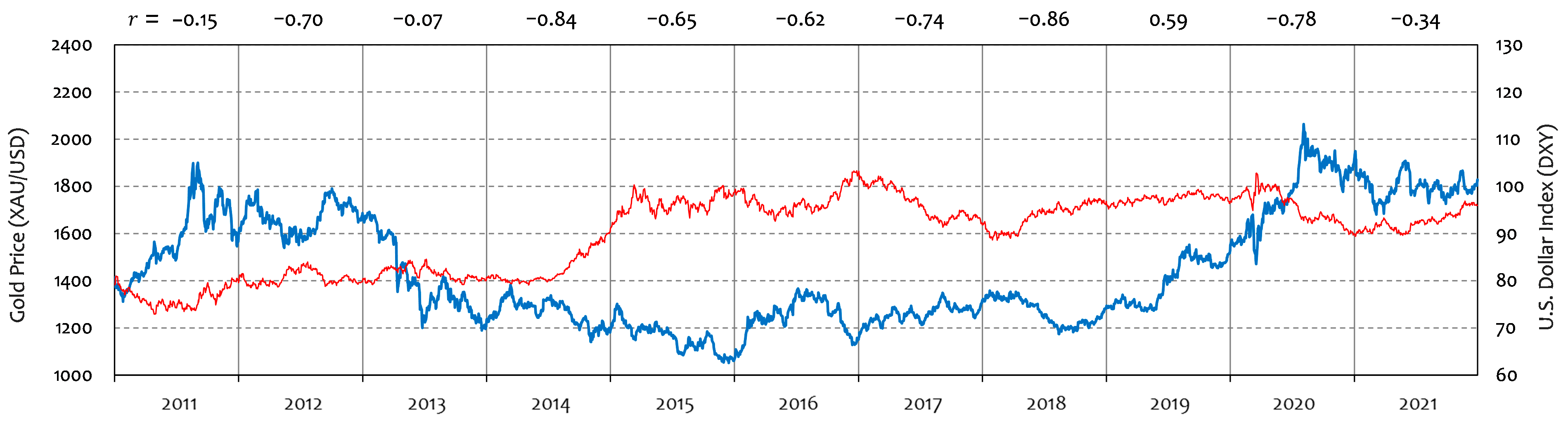
From 2011 to 2018, gold prices experienced several notable cycles driven by shifts in global macroeconomic conditions. In 2011, prices reached an all-time high near $1900 amid heightened uncertainty related to the European debt crisis and the U.S. credit rating downgrade. Prices subsequently retreated in 2012–2013, fluctuating between $1200 and $1800 as the Federal Reserve initiated and later signaled the tapering of quantitative easing. Gold continued to decline through 2014–2015, as expectations of U.S. rate hikes contributed to a stronger dollar.

During 2016–2018, gold generally moved inversely to the dollar, with price fluctuations influenced by events such as the Brexit referendum, rising U.S.–China trade tensions, and diverging central bank policies. These movements illustrate the typical inverse relationship between gold and the dollar observed throughout most of this period.

Starting in 2019, however, gold exhibited atypical behavior. Renewed concerns over a global economic slowdown lifted gold to the mid-$1500s, producing an unusual positive gold–dollar correlation (r = 0.59) as both assets strengthened amid heightened risk aversion. Gold then surged above $2000 in 2020 during the COVID-19 pandemic, before stabilizing within the mid-$1700s to mid-$1800s range in 2021. Over the full period (2011–2021), the gold–dollar relationship was mildly negative (r = −0.28), consistent with gold’s long-term tendency to move inversely to the U.S. dollar (see Figure 2 for the yearly correlation values).

Collectively, these episodes span several distinct macroeconomic and financial regimes relevant to gold markets, making the sample period appropriate for examining the performance of trend-following technical indicators such as the MACD.

4.1. Results of In-Sample Tests

Table 1. Summary statistics of in-sample test results (2011–2019).

		n	Max	Min	Mean	Median	S.D.	Skewness	Kurtosis
Optimal Groups	An1–An2–An3	180	0.2778	$-$0.2611	0.0086	0.0098	0.1398	$-$0.0031	$-$1.0711
	An1–An2–Bn3	80	0.6615	$-$0.0418	0.3380	0.3736	0.2050	$-$0.2297	$-$1.4722
	An1–Bn2–An3	360	0.6082	$-$0.0610	0.3803	0.4153	0.1511	$-$0.8376	$-$0.0829
	An1–Bn2–Bn3	160	0.5471	0.2578	0.3785	0.3573	0.0751	0.4713	$-$0.7746
Non-optimal Groups	Wn1–Wn2–Wn3	35	0.2671	$-$0.3915	$-$0.1167	$-$0.1116	0.1480	0.2849	0.2020
	Wn1–Xn2–Wn3	80	0.0763	$-$0.2768	$-$0.0951	$-$0.1166	0.0837	0.1485	$-$0.7073

Note: “n” indicates the number of sample models in each group, and “S.D.” denotes the standard deviation.

presents summary statistics for the newly constructed sample models with parameter values falling within the predefined optimal and non-optimal ranges. The results reveal a clear and systematic performance contrast between the optimal and non-optimal groups.

All optimal model groups—A_n1–A_n2–A_n3, A_n1–A_n2–B_n3, A_n1–B_n2–A_n3, and A_n1–B_n2–B_n3— exhibit positive mean returns. Among these, the A_n1–B_n2–B_n3 group shows uniformly positive returns (Max = 0.5471, Min = 0.2578) with the smallest dispersion (S.D. = 0.0751), indicating the most stable and consistently strong profitability under this parameter configuration. In contrast, the non-optimal groups—W_n1–W_n2–W_n3 and W_n1–X_n2–W_n3—exhibit negative mean returns, reflecting systematic underperformance when parameters fall within the non-optimal ranges. This clear contrast between the two sets of groups suggests that a model’s performance is closely linked to parameter configuration.

4.2. Results of Out-of-Sample Tests

Table 2. Summary statistics of out-of-sample test results (2020–2021).

		n	Max	Min	Mean	Median	S.D.	Skewness	Kurtosis
Optimal Groups	An1–An2–An3	180	0.1241	$-$0.2629	$-$0.1100	$-$0.1450	0.0979	0.9567	$-$0.0900
	An1–An2–Bn3	80	0.1967	0.0055	0.1038	0.1063	0.0467	$-$0.3156	$-$0.7568
	An1–Bn2–An3	360	0.2088	0.0055	0.1184	0.1235	0.0463	$-$0.2269	$-$0.6281
	An1–Bn2–Bn3	160	0.1518	0.0318	0.0759	0.0713	0.0274	1.2364	1.3171
Non-optimal Groups	Wn1–Wn2–Wn3	35	0.1918	$-$0.4263	$-$0.1506	$-$0.2255	0.0300	0.8046	$-$0.7287
	Wn1–Xn2–Wn3	80	$-$0.1801	$-$0.5721	$-$0.4296	$-$0.4533	0.0123	0.8202	$-$0.3670

summarizes the out-of-sample performance of the sample models. Three of the four optimal model groups—A_n1–A_n2–B_n3, A_n1–B_n2–A_n3, and A_n1–B_n2–B_n3—maintain positive mean returns, consistent with their in-sample performance. Focusing on the “Min” column, all models in these three groups exhibit exclusively positive returns, indicating that their profitability and parameter configurations remain robust when applied to out-of-sample data not used for model estimation. However, the A_n1–A_n2–A_n3 group records a negative mean return of −0.1100, in contrast to its previously positive in-sample result. This deterioration appears attributable to the group’s relatively shorter n₃ values, which make its performance more sensitive to market fluctuations.

By contrast, both non-optimal groups—W_n1–W_n2–W_n3 and W_n1–X_n2–W_n3—continue to produce negative mean returns. Notably, the latter group—W_n1–X_n2–W_n3— exhibits a particularly large mean loss of −0.4296. None of the models in this group produce a positive return; all outcomes are negative, ranging from a maximum of −0.1801 to a minimum of −0.5721.

Overall, with the exception of the A_n1–A_n2–A_n3 group, the broad consistency between in-sample and out-of-sample results across the optimal groups provides empirical evidence for their relative effectiveness. These findings indicate that the proposed methodology successfully identifies optimal and non-optimal parameter ranges in the gold market, while clearly distinguishing the systematic underperformance of the non-optimal groups.

Given the inconsistent and relatively weak performance of the A_n1–A_n2–A_n3 group across the two test periods, this study excludes this group from the main discussion, although its results are retained in the subsequent analysis for completeness. By contrast, the persistently poor performance of the non-optimal groups is clearly established; accordingly, these models are excluded from further discussion.

4.3. A Closer Examination of Model Robustness

Although the robustness of the optimal model groups has been confirmed in the previous sections, a closer inspection of the “Min” column in Table 1 and Table 2 reveals a potential issue. In the A_n1–A_n2–B_n3 and A_n1–B_n2–A_n3 groups, minimum returns are negative in the in-sample test (Table 1; −0.0418 and −0.0610) but positive in the out-of-sample test (Table 2; both 0.0055). This pattern indicates that some models produced negative in-sample but positive out-of-sample returns, raising questions as to whether their parameter settings can be regarded as consistently optimal. To identify models that remain robust across both periods, this study examines how many models in these two groups recorded negative in-sample returns and to refine the analysis by excluding these cases.

Table 3. Performance classification of sample models in the optimal groups (2011–2021).

	P-P		P-N		N-P		N-N		Total
	n	Ratio	n	Ratio	n	Ratio	n	Ratio	n	Ratio
An1–An2–An3	34	(18.9%)	63	(35.0%)	0	(0.0%)	83	(46.1%)	180	(100.0%)
An1–An2–Bn3	79	(98.8%)	0	(0.0%)	1	(1.2%)	0	(0.0%)	80	(100.0%)
An1–Bn2–An3	356	(98.9%)	0	(0.0%)	4	(1.1%)	0	(0.0%)	360	(100.0%)
An1–Bn2–Bn3	160	(100.0%)	0	(0.0%)	0	(0.0%)	0	(0.0%)	160	(100.0%)

Note: P-P and N-N denote the number of models with consistently positive or consistently negative returns, respectively, in both in-sample and out-of-sample tests. P-N and N-P indicate the number of models for which the sign of returns differs between the two tests.

reports the number of models in the four optimal groups that generated positive returns in both the in-sample and out-of-sample tests. In the A_n1–A_n2–B_n3 group, 79 models are classified as P-P, while only one model falls into the N-P category. This indicates that, even when this single N-P model is excluded and attention is restricted to the large set of P-P models, the robustness of the corresponding parameter configuration remains essentially unchanged. A similar pattern is observed for the A_n1–B_n2–A_n3 group, which contains 356 P-P models and only 4 N-P models. Notably, all models in the A_n1–B_n2–B_n3 group are classified as P-P, indicating particularly strong robustness within this group.

In contrast, for completeness, it should be noted that the A_n1–A_n2–A_n3 group contains only 34 P-P models, indicating limited robustness relative to the other optimal groups. Excluding this group, 99.2% of the models in the remaining three groups (595 out of 600) are classified as P-P. This high degree of consistency across both test periods supports the robustness of their parameter settings and motivates a more detailed examination of the characteristics shared by P-P models within each group.

4.4. Overview of P–P Model Performance

Building on the robustness analysis presented above, the performance of P-P models in each group is evaluated in terms of both profitability and stability.

Table 4. Performance statistics of P-P models in the optimal groups (2011–2021).

	n (P-P)	Max	Min	Mean	Median	S.D.	Skewness	Kurtosis
An1–An2–An3	34	0.3971	0.0848	0.2604	0.2485	0.0754	$-$0.1348	$-$0.4377
An1–An2–Bn3	79	0.7914	0.0059	0.4479	0.5311	0.2329	$-$0.4329	$-$1.3304
An1–Bn2–An3	356	0.7804	0.0071	0.5042	0.5546	0.1700	$-$0.9503	0.2950
An1–Bn2–Bn3	160	0.6989	0.2984	0.4544	0.4258	0.0925	0.6736	$-$0.2123

Note: The “mean” represents the average of the total return accumulated by each model over the entire sample period.

summarizes their performance over the full test period and facilitates a comparison of overall return levels, variability, and distributional characteristics.

Focusing first on profitability, the A_n1–B_n2–A_n3 group records the highest mean return (0.5042), indicating that, on average, it contains models achieving relatively high returns. However, its higher standard deviation (0.1700) and pronounced negative skewness (−0.9503) imply greater variability and a higher likelihood of occasional low-return outcomes, consistent with its wide max–min range (0.7804–0.0071).

In contrast, the A_n1–B_n2–B_n3 group exhibits a more stable performance profile. Its lower standard deviation (0.0925) and positive skewness (0.6736) indicate a more concentrated return distribution tilted toward higher returns, while its relatively narrow max–min range (0.6989–0.2984) further supports this interpretation. Moreover, its comparatively high minimum return (0.2984) suggests that even the weakest models in this group outperform those in the other groups.

Taken together, these results indicate that while the A_n1–B_n2–A_n3 group achieves the highest average profitability, the A_n1–B_n2–B_n3 group offers a more favorable balance between return and stability. This suggests that the parameter settings in A_n1–B_n2–B_n3 tend to deliver steadier performance across models. For a more detailed assessment of robustness, the annual performance of the P-P models is examined on a year-by-year basis.

4.5. Annual Performance of P-P Models

Before proceeding to the year-by-year analysis of the P-P model performance, this study introduces a measure specifically designed for this purpose, termed the Directional Return Imbalance (DRI). The DRI is designed to assess whether market conditions in a given year are more favorable to long or short trading positions, by summarizing the balance between cumulative upward and downward price movements. It thus provides a concise indicator of the market’s overall directional bias during the year. It is formalized as follows:

$$\mathrm{Directional} \mathrm{Return} \mathrm{Imbalance} (\mathrm{DRI}) ={\displaystyle \frac{{\sum }_{t\in \mathit{T}, d_{t>0}}{d}_t}{{\sum }_{t\in \mathit{T}, d_{t<0}}\left|d_t\right|}} , d_t={\displaystyle \frac{P_t}{P_{t-1}}}-1$$

(5)

where T denotes the set of all trading days in a given year. The numerator (denominator) represents the cumulative sum of positive (negative) daily returns, capturing the aggregate strength of upward (downward) price movements over the year. Here, $d_t$ denotes the simple daily return, and $P_t$ is the closing price on day t.

The DRI index is interpreted as follows. When DRI > 1, cumulative upward price movements dominate downward movements, indicating a market environment more favorable to long positions. Conversely, when DRI < 1, downward movements dominate, favoring short positions.

The year-by-year DRI values at the top of

Table 5. Year-by-Year Performance of P-P Models by Position Type (Long, Short, and Combined).

	2011	2012	2013	2014	2015	2016	2017	2018	2019	2020	2021	Ave	Total
DRI	1.105	1.099	0.775	0.991	0.889	1.106	1.219	0.982	1.289	1.244	0.966	$-$	$-$
[a] An1–An2–An3
Long	0.111	$-$0.011	$-$0.182	$-$0.106	$-$0.006	0.101	0.057	$-$0.018	0.082	0.064	0.044	0.012	0.1351
Short	$-$0.083	$-$0.010	0.158	0.024	0.088	0.041	0.040	0.007	$-$0.095	$-$0.119	0.074	0.011	0.1253
L&S	0.028	$-$0.021	$-$0.025	$-$0.082	0.081	0.142	0.097	$-$0.011	$-$0.013	$-$0.055	0.119	0.024	0.2604
[b] An1–An2–Bn3
Long	0.126	0.040	$-$0.183	$-$0.071	$-$0.031	0.096	0.047	$-$0.011	0.086	0.076	0.032	0.019	0.2068
Short	$-$0.050	0.038	0.176	0.024	0.062	0.038	0.034	0.015	$-$0.093	$-$0.060	0.057	0.022	0.2410
L&S	0.076	0.078	$-$0.008	$-$0.047	0.031	0.134	0.081	0.004	$-$0.007	0.016	0.089	0.041	0.4479
[c] An1–Bn2–An3
Long	0.121	0.044	$-$0.189	$-$0.062	$-$0.029	0.094	0.050	$-$0.011	0.094	0.086	0.029	0.021	0.2266
Short	$-$0.040	0.041	0.170	0.030	0.064	0.036	0.040	0.017	$-$0.084	$-$0.048	0.052	0.025	0.2776
L&S	0.081	0.085	$-$0.019	$-$0.032	0.035	0.129	0.090	0.006	0.010	0.038	0.081	0.046	0.5042
[d] An1–Bn2–Bn3
Long	0.099	0.054	$-$0.222	$-$0.036	$-$0.026	0.094	0.031	$-$0.018	0.136	0.084	$-$0.015	0.016	0.1807
Short	$-$0.043	0.048	0.123	0.039	0.069	0.031	0.023	0.022	$-$0.045	0.008	$-$0.001	0.025	0.2737
L&S	0.057	0.102	$-$0.100	0.003	0.042	0.125	0.054	0.005	0.091	0.092	$-$0.016	0.041	0.4544

Note: The “Ave” column reports the average of the annual per-model returns shown in each group. The “Total” column reports the cumulative per-model return over the entire sample period, corresponding to the “mean” values reported in Table 4.

show substantial variation in market directional conditions, as also reflected in Figure 1. Years with DRI > 1 are observed in six years (2011, 2012, 2016, 2017, 2019, and 2020), with particularly high values in 2017, 2019, and 2020, where the DRI exceeds unity by roughly 20–30%. In contrast, years with DRI < 1 are observed in the remaining five years (2013, 2014, 2015, 2018, and 2021).

Analysis of model performance under these DRI-defined market conditions reveals a clear pattern. In years with DRI > 1, long-side returns are positive across all three model groups—A_n1–A_n2–B_n3, A_n1–B_n2–A_n3, and A_n1–B_n2–B_n3—and consistently exceed the corresponding short-side returns. Conversely, in years with DRI < 1, short-side returns dominate, confirming a relative advantage of short positions under such conditions.

Overall, these findings demonstrate that, on average across models in each group, the P-P models capture the prevailing market direction, performing better through long positions in upward-biased years and through short positions in downward-biased years. These patterns are not driven by trading frequency imbalances, as the numbers of long and short positions are nearly identical across models.

Focusing on the combined long-and-short (L&S) returns reported in Table 5, the A_n1–A_n2–B_n3 group records negative L&S returns in three years (2013, 2014, and 2019), compared with two years (2013 and 2014) for the A_n1–B_n2–A_n3 group and two years (2013 and 2021) for the A_n1–B_n2–B_n3 group. Outside these years, all three groups generate positive L&S returns over the remaining years of the eleven-year sample period.

It is also worth noting the performance of the three optimal model groups during the COVID-19 crisis period. Their accumulated long-and-short (L&S) returns over 2020–2021 are all positive, suggesting that the P-P models perform well not only during relatively normal market conditions but also during periods of heightened market stress.

These findings raise the possibility that gold-based trading strategies may have contributed to offsetting losses in other asset classes—such as stock markets—or, in turn, to enhancing overall portfolio performance during much of the sample period. For example, Kang (2023) documents that P-P model-based trading strategies applied to three stock index futures recorded negative returns in multiple years over the same period, including 2011 and 2017 for the Nikkei; 2011, 2012, and 2015 for the Dow Jones; and 2011, 2012, 2017, and 2018 for the Nasdaq. In contrast, the L&S returns of the three gold-based optimal model groups in this study remain positive in those same years.

However, the DRI is a descriptive indicator of market direction rather than a causal determinant of model performance. Accordingly, these findings are suggestive rather than conclusive and do not imply that gold-based strategies consistently hedge stock market losses.

4.6. Impact of Stop-Loss and Profit-Target Settings on P–P Model Performance

The remaining question is whether the P-P models maintain their performance under stop-loss and take-profit rules. To investigate this question, the following rules were applied to the P-P models: an open position was closed when it reached either a loss of 5% or 10% (stop-loss) or a profit of 5% or 10% (take-profit), relative to the entry price. Among the four possible threshold combinations—5%/5%, 10%/5%, 10%/10%, and 5%/10%—the latter two produced more favorable results than the first two. For brevity, the discussion below focuses on the results obtained under the 10%/10% and 5%/10% settings.

Table A1. P-P Model Returns with 10% Stop-Loss and 10% Profit-Target.

10%/10%	2011	2012	2013	2014	2015	2016	2017	2018	2019	2020	2021	Ave	Total
[a] An1–An2–An3
Long	0.068	$-$0.012	$-$0.169	$-$0.106	$-$0.006	0.041	0.057	$-$0.018	0.098	0.067	0.053	0.006	0.0714
Short	$-$0.004	$-$0.042	0.205	0.024	0.088	0.041	0.040	0.007	$-$0.095	$-$0.119	0.074	0.020	0.2190
L&S	0.064	$-$0.054	0.036	$-$0.082	0.082	0.081	0.097	$-$0.011	0.003	$-$0.052	0.127	0.026	0.2905
[b] An1–An2–Bn3
Long	0.077	0.041	$-$0.157	$-$0.071	$-$0.031	0.050	0.047	$-$0.011	0.097	0.081	0.040	0.015	0.1623
Short	0.068	$-$0.023	0.221	0.024	0.062	0.038	0.034	0.015	$-$0.093	$-$0.060	0.057	0.031	0.3420
L&S	0.145	0.018	0.064	$-$0.047	0.030	0.088	0.081	0.004	0.003	0.021	0.097	0.046	0.5043
[c] An1–Bn2–An3
Long	0.070	0.054	$-$0.155	$-$0.062	$-$0.029	0.050	0.050	$-$0.011	0.102	0.091	0.039	0.018	0.1992
Short	0.088	$-$0.020	0.213	0.030	0.064	0.036	0.040	0.017	$-$0.084	$-$0.048	0.052	0.035	0.3861
L&S	0.158	0.035	0.058	$-$0.032	0.035	0.085	0.090	0.006	0.018	0.043	0.090	0.053	0.5852
[d] An1–Bn2–Bn3
Long	0.054	0.065	$-$0.155	$-$0.036	$-$0.026	0.046	0.031	$-$0.018	0.128	0.084	0.011	0.017	0.1837
Short	0.120	$-$0.005	0.163	0.039	0.069	0.031	0.023	0.022	$-$0.045	0.008	$-$0.001	0.039	0.4239
L&S	0.173	0.060	0.008	0.003	0.042	0.077	0.054	0.005	0.083	0.092	0.010	0.055	0.6076

and

Table A2. P-P Model Returns with 5% Stop-Loss and 10% Profit-Target.

5%/10%	2011	2012	2013	2014	2015	2016	2017	2018	2019	2020	2021	Ave	Total
[a] An1–An2–An3
Long	0.073	$-$0.002	$-$0.125	$-$0.116	$-$0.013	0.034	0.061	$-$0.032	0.076	0.046	0.052	0.005	0.0548
Short	0.018	$-$0.045	0.193	0.014	0.081	0.026	0.040	$-$0.008	$-$0.086	$-$0.104	0.112	0.022	0.2421
L&S	0.092	$-$0.047	0.068	$-$0.102	0.068	0.060	0.102	$-$0.040	$-$0.010	$-$0.057	0.164	0.027	0.2969
[b] An1–An2–Bn3
Long	0.087	0.044	$-$0.105	$-$0.071	$-$0.031	0.061	0.047	$-$0.011	0.081	0.081	0.054	0.021	0.2363
Short	0.071	$-$0.023	0.222	0.024	0.062	0.038	0.034	0.015	$-$0.092	$-$0.060	0.110	0.036	0.4003
L&S	0.158	0.020	0.117	$-$0.047	0.030	0.099	0.081	0.004	$-$0.011	0.021	0.163	0.058	0.6366
[c] An1–Bn2–An3
Long	0.076	0.055	$-$0.105	$-$0.062	$-$0.029	0.059	0.050	$-$0.011	0.094	0.091	0.055	0.025	0.2734
Short	0.089	$-$0.020	0.217	0.030	0.064	0.035	0.040	0.017	$-$0.083	$-$0.048	0.104	0.040	0.4435
L&S	0.165	0.036	0.112	$-$0.033	0.035	0.094	0.090	0.006	0.010	0.043	0.159	0.065	0.7169
[d] An1–Bn2–Bn3
Long	0.054	0.065	$-$0.105	$-$0.035	$-$0.026	0.050	0.031	$-$0.018	0.127	0.084	0.031	0.024	0.2593
Short	0.120	$-$0.005	0.169	0.039	0.069	0.000	0.023	0.022	$-$0.045	0.008	0.056	0.041	0.4563
L&S	0.173	0.060	0.065	0.005	0.042	0.050	0.054	0.005	0.083	0.092	0.087	0.065	0.7156

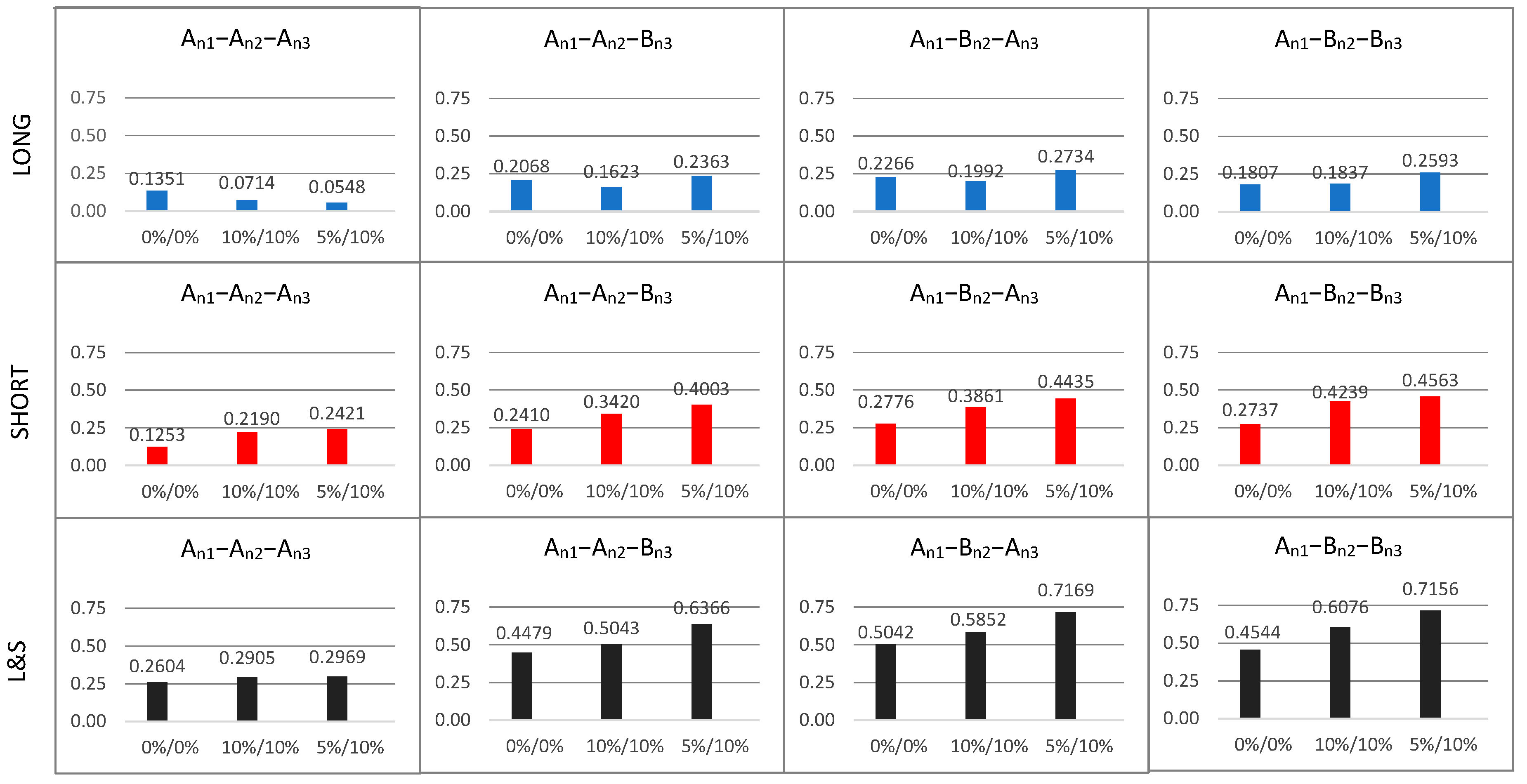
present the detailed simulation results for the two scenarios. To help readers grasp the main findings prior to engaging with the full set of numerical results, Figure 3 is presented first in the main text as a concise summary. For reasons of presentation, the detailed results in Table A1 and Table A2 are reported in the Appendix A. Figure 3 compares the “Total” results (rightmost column) for the Long, Short, and L&S categories with the corresponding values from Table 5 and those reported in Table A1 and Table A2.

Starting with the long-trade performance (blue) shown at the top of Figure 3, both the 10%/10% and 5%/10% rules reduced returns for the leftmost A_n1–A_n2–A_n3 group, which has already been excluded from the main discussion due to its inconsistent and relatively weak performance across the two test periods. For the remaining three groups—A_n1–A_n2–B_n3, A_n1–B_n2–A_n3, and A_n1–B_n2–B_n3—the 10%/10% rule provided little or no improvement over the 0%/0% case, whereas the 5%/10% rule generated modest but consistent gains.

Turning to the short-trade performance (red) in the middle of Figure 3, both the 10%/10% and 5%/10% exit rules improved performance across all four model groups, with the 5%/10% rule consistently delivering larger gains.

Finally, for the L&S performance (black) shown at the bottom of Figure 3, the 5%/10% rule improved total returns across all four groups, with incremental gains that were particularly notable in A_n1–A_n2–B_n3, A_n1–B_n2–A_n3, and A_n1–B_n2–B_n3.

Overall, the 5%/10% rule outperformed the 10%/10% rule. However, neither exit rule produced a meaningful improvement in overall returns for the A_n1–A_n2–A_n3 group. These results suggest that the effectiveness of exit rules depends critically on the model’s parameter configuration, indicating that exit-rule design alone is insufficient unless the underlying parameter combination is already close to optimal for the prevailing market environment.

Table 6. Comparison of P–P Model Returns With and Without Stop-Loss and Profit-Target Exit Rules.

	An1–An2–Bn3			An1–Bn2–An3			An1–Bn2–Bn3
	Ave	Std.D.	Sharpe R.	Ave	Std.D.	Sharpe R.	Ave	Std.D.	Sharpe R.
Strategy A (0%/0%)	0.041	0.054	0.748	0.046	0.051	0.893	0.041	0.065	0.638
Strategy B (10%/10%)	0.046	0.054	0.843	0.053	0.051	1.038	0.055	0.051	1.078
Strategy C (5%/10%)	0.058	0.070	0.827	0.065	0.064	1.020	0.065	0.046	1.407

Note: Annual average log returns (Ave), standard deviations (Std.D.), and Sharpe ratios (Sharpe R.) are computed from the L&S returns for each model group over 2011–2021 (11 annual observations), reported in Table 5 for Strategy A and in Table A1 and Table A2 for Strategies B and C, respectively.

provides a quantitative comparison of returns under the three exit-rule strategies for the three model groups, excluding A_n1–A_n2–A_n3. Focusing on the “Ave” and “Sharpe R.” columns, Strategies B and C consistently outperform Strategy A in terms of both average returns and risk-adjusted performance.

A comparison across model groups reveals an interesting pattern. Prior to the application of exit rules (Strategy A), the A_n1–B_n2–A_n3 group exhibits stronger performance, with a higher Sharpe ratio (0.893) than the A_n1–B_n2–B_n3 group (0.638). However, once exit rules are introduced, the performance improvements associated with Strategies B and C are more pronounced for the A_n1–B_n2–B_n3 group. Notably, the highest Sharpe ratio (1.407) is achieved under Strategy C within this model group.

Focusing on the A_n1–B_n2–B_n3 model group highlights the quantitative impact of the two exit-rule strategies. Relative to Strategy A (i.e., before the application of exit rules), Strategy B delivers a 1.7-fold increase in risk-adjusted returns, as reflected in the Sharpe ratio (1.078 vs. 0.638), while reducing risk by approximately 22%, based on the standard deviation. Strategy C further enhances performance, achieving a 2.2-fold increase in the Sharpe ratio (1.407 vs. 0.638) together with an approximately 29% reduction in risk.

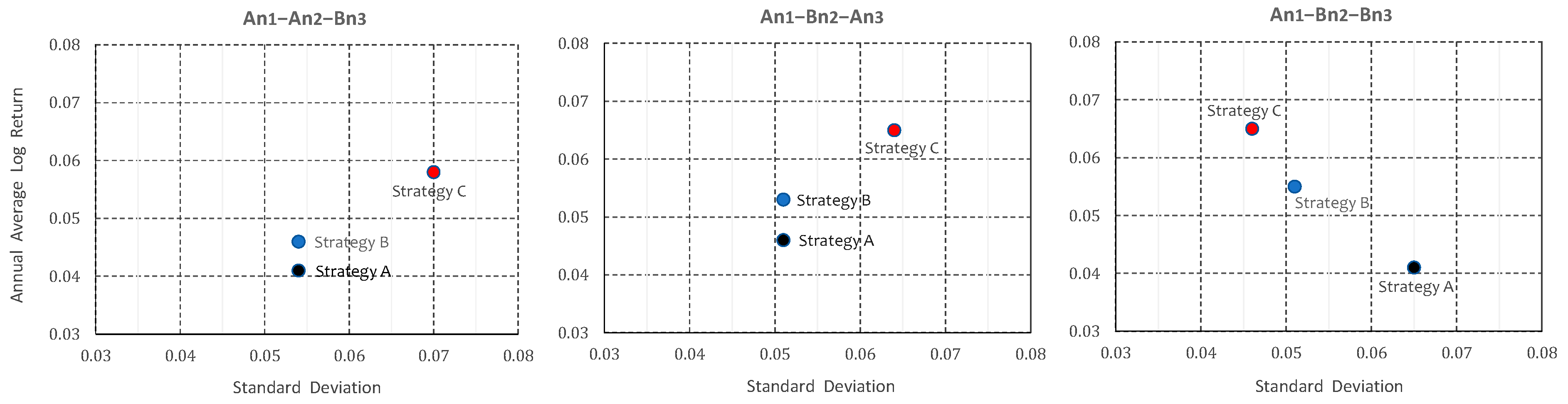
Figure 4 illustrates these effects most clearly for the A_n1–B_n2–B_n3 model group, where Strategy C is positioned to reflect both higher returns and lower risk, visually reinforcing the overall advantage of this configuration.

To summarize, the combination of the models in this group and Strategy C (5%/10%) achieves a favorable balance between risk control and profit realization, delivering the strongest improvement in risk-adjusted performance in the gold market over the study period.

4.7. Statistical Robustness Test Results

This section presents the results of robustness tests examining whether the performance of the four optimal P-P model groups is statistically superior to that of the conventional MACD (12,26,9) model. The conventional model is adopted as a benchmark rather than a simple buy-and-hold strategy, since all P-P models are derived from the MACD framework and aim to identify optimal parameter configurations, making the MACD (12,26,9) specification a natural point of comparison.

For the robustness tests, annual log returns over an 11-year period (L&S) for each of the four optimal P-P model groups were compared against those of the benchmark MACD model. Returns for Strategy A (0%/0%) and Strategy C (5%/10%) are reported in Table 5 and Table A2, respectively. A one-sided paired t-test was conducted to determine whether ${\mu }_d$, the mean difference in annual returns between each P-P model group and the benchmark model, was significantly greater than zero ($H_0: {\mu }_d=0$ against $H_1: {\mu }_d>0$).

Panel (a) of

Table 7. Robustness Test Results for the P-P Model Groups versus the Benchmark MACD (12,26,9) Model.

	2011	2012	2013	2014	2015	2016	2017	2018	2019	2020	2021	Ave	t-Stat	p
Panel [a]: Results with Stop-loss and Profit-target Rules (5%/10%)
12–26–9	0.167	−0.036	0.032	−0.186	0.139	−0.028	0.069	−0.096	−0.060	−0.090	0.096	0.001	-	-
A–A–A	0.092	−0.047	0.068	−0.102	0.068	0.060	0.102	−0.040	−0.010	−0.057	0.164	0.027 ^	1.555	0.076
A–A–B	0.158	0.020	0.117	−0.047	0.030	0.099	0.081	0.004	−0.011	0.021	0.163	0.058 *	2.660	0.012
A–B–A	0.165	0.036	0.112	−0.033	0.035	0.094	0.090	0.006	0.010	0.043	0.159	0.065 **	2.958	0.007
A–B–B	0.173	0.060	0.065	0.005	0.042	0.050	0.054	0.005	0.083	0.092	0.087	0.065 *	2.382	0.019
Panel [b]: Results without Stop-loss and Profit-target Rules (0%/0%)
12–26–9	0.071	0.029	−0.076	−0.186	0.139	0.006	0.069	−0.096	−0.062	−0.138	0.009	−0.021	-	-
A–A–A	0.028	−0.021	−0.025	−0.082	0.081	0.142	0.097	−0.011	−0.013	−0.055	0.119	0.024 *	2.194	0.026
A–A–B	0.076	0.078	−0.008	−0.047	0.031	0.134	0.081	0.004	−0.007	0.016	0.089	0.041 **	2.766	0.010
A–B–A	0.081	0.085	−0.019	−0.032	0.035	0.129	0.090	0.006	0.010	0.038	0.081	0.046 **	2.910	0.008
A–B–B	0.057	0.102	−0.100	0.003	0.042	0.125	0.054	0.005	0.091	0.092	−0.016	0.041 *	1.991	0.037

Note: ^, *, and ** denote statistical significance at the 10%, 5%, and 1% levels, respectively, based on one-tailed tests. t-Stat and p represent t-statistic and p-value. “12–26–9” refers to the benchmark MACD (12, 26, 9), whose annual returns were computed specifically for this test. Group labels A–A–A, A–A–B, A–B–A, and A–B–B correspond to the A_n1–A_n2–A_n3, A_n1–A_n2–B_n3, A_n1–B_n2–A_n3, and A_n1–B_n2–B_n3 model groups, respectively.

presents the statistical significance of the four P-P model groups’ performance relative to the MACD (12,26,9) model when stop-loss and profit-target rules (5%/10%) are applied. The results clearly show that all four model groups significantly outperform the benchmark at conventional significance levels. Among them, the three groups—A_n1–A_n2–B_n3, A_n1–B_n2–A_n3, and A_n1–B_n2–B_n3—exhibit even stronger significance, reaching the 5% or 1% level, highlighting their robust and consistent advantage over the so-called standard MACD specification.

Panel (b) further shows that this statistically significant outperformance is consistently observed across all model groups, even without the use of stop-loss or profit-target rules. Taken together, these results indicate that the P-P model groups’ superiority is robust and not solely attributable to the implementation of exit rules, emphasizing the pivotal role of parameter optimization within the MACD framework.

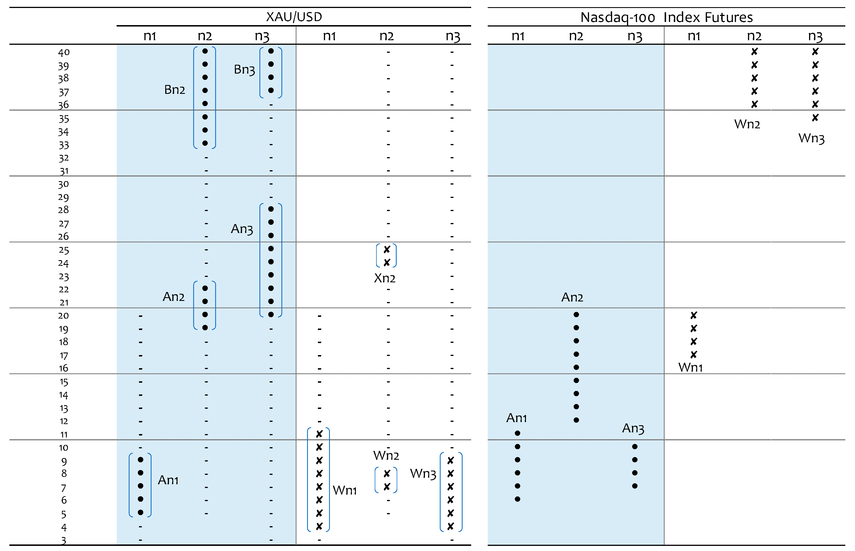
4.8. Characteristics of Optimal and Non-Optimal Parameter Ranges in Gold and Stock Markets

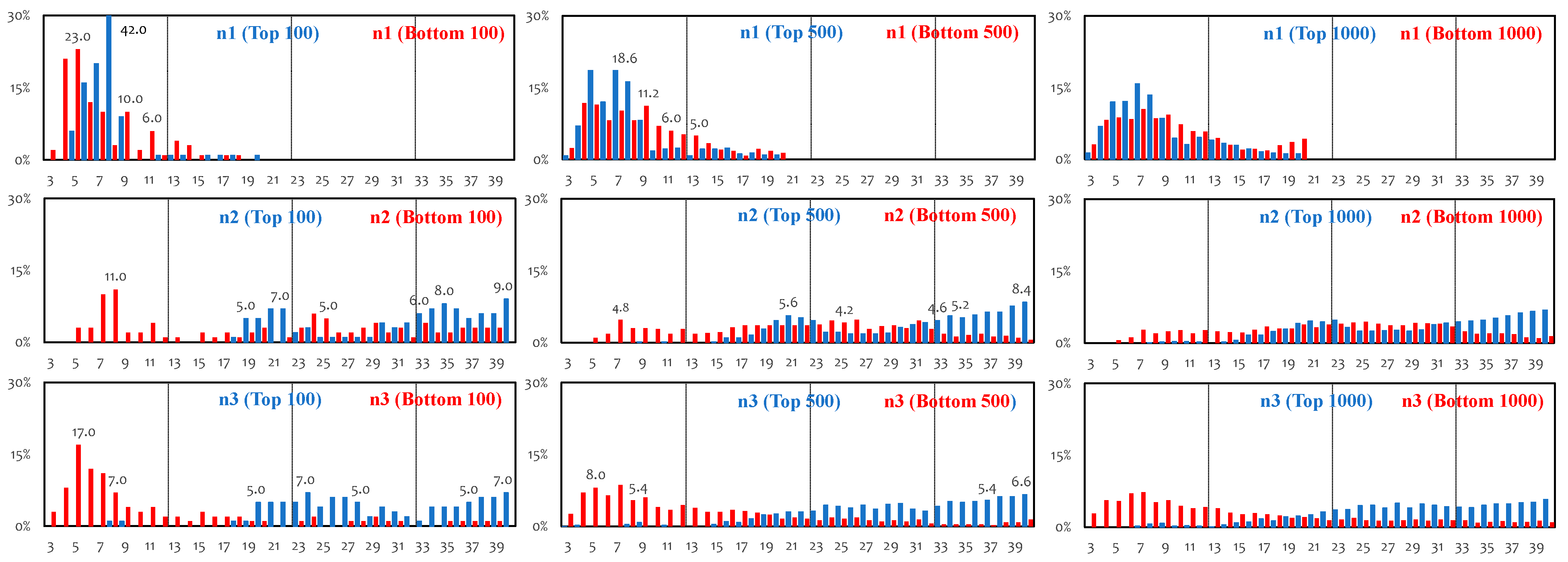
This section addresses the research question posed in the Introduction by comparing the distributions of optimal and non-optimal MACD parameter value ranges in the gold market with those reported for the stock market by Kang (2023).2 Several key observations can be drawn from Figure 5.

(1)

Non-optimal parameter value ranges:

In the gold market (left panel), the non-optimal parameter ranges—corresponding to the W_n1–W_n2–W_n3 and W_n1–X_n2–W_n3 groups—are characterized by relatively small values of n₁, n₂ and n₃. These settings result in shorter MACD and signal lines, leading to more frequent, short-horizon trading signals. Given that these parameter combinations yield negative mean returns in both in-sample and out-of-sample tests, they appear unsuitable for the gold market. By contrast, in the stock market (right panel), the non-optimal parameter ranges—W_n1–W_n2–W_n3—are associated with relatively large values of n₁, n₂ and n₃, implying longer MACD and signal lines and, consequently, less frequent, longer-horizon signals.

These findings indicate that overly short-term MACD parameter settings are unsuitable for the gold market, whereas overly long-term settings are inappropriate for the stock market.

(2)

Optimal parameter value ranges:

• Compared with the A_n1–A_n2–A_n3 group models in the gold market, the high-performing A_n1–B_n2–B_n3 group models use larger n₂ and n₃ values (i.e., A_n2 < Bn₂ and A_n3 < Bn₃), resulting in longer MACD and signal lines. Since the A_n1–B_n2–B_n3 group outperforms the A_n1–A_n2–A_n3 group, this parameter configuration appears to be a key factor in their superior performance.
• Similarly, the A_n1–A_n2–B_n3 and A_n1–B_n2–A_n3 models extend either the MACD or the signal line and outperform the A_n1–A_n2–A_n3 group. This suggests that lengthening either component can improve gold returns.
• Overall, the A_n1–B_n2–B_n3 group represents an optimal degree of parameter extension, with both MACD and signal lines lengthened. The parameter ranges shown in Figure 5 appear to be essential for capturing medium- to long-term gold price movements, consistent with the strong risk-adjusted performance observed when combined with Strategy C (5%/10%).
• A particularly noteworthy cross-market contrast emerges. Despite substantial overlap in n₂ and n₃ ranges between the A_n1–B_n2–B_n3 group in the gold market and the non-optimal W_n1–W_n2–W_n3 group in the stock market, differences in n₁ alone lead to opposite outcomes. Small n₁ values (5 ≤ n₁ ≤ 9) yield the best performance in gold, whereas large n₁ values (17 ≤ n₁ ≤ 20) yield the worst performance in the stock market. This indicates that MACD performance depends on the joint configuration of n₁, n₂, and n₃ rather than on individual parameters, reflecting differences in underlying price dynamics across the two markets.

(3)

Market-Specific Implications of MACD Parameter Ranges:

A cross-market comparison of the optimal parameter ranges for the A_n1–B_n2–B_n3 group in gold and the A_n1–A_n2–A_n3 group models in the stock market highlights differences in the investment horizons implied by MACD parameter choices. The average number of trades over the 11-year period is 129.8 for the A_n1–B_n2–B_n3 group in gold and 274.6 for the A_n1–A_n2–A_n3 group in the stock market (Kang, 2023), corresponding to approximately 0.98 trades per month for gold and 2.08 trades per month for the stock market. These results suggest that MACD parameter optimization differs across markets not only in parameter values but also in signal-generation dynamics—favoring relatively shorter-term strategies in the stock market and medium- to long-term approaches in gold.

5. Summaries and Concluding Remarks

This study begins with a simple question: whether optimal and non-optimal MACD parameter ranges can be identified for the gold market. To address this question, the framework for selecting optimal and non-optimal parameter values proposed by Kang (2023) is applied to the gold market. The results demonstrate that this methodological framework is effective in the gold market as well. Beyond validating the methodology and identifying optimal and non-optimal MACD parameter ranges in the gold market, this study provides several important implications for both market participants and researchers. Before discussing these broader implications, the main empirical findings are summarized below.

• Main empirical findings
  • The clear contrast in performance between model groups with identified optimal and non-optimal parameter values, observed almost consistently in both in-sample and out-of-sample tests, highlights the importance of parameter configuration effects in MACD-based trading strategies. By explicitly identifying optimal and non-optimal parameter ranges in the gold market, this study demonstrates that performance differences emerge systematically at the group level and are linked to specific parameter combinations (Section 4.1 and Section 4.2)
  • Focusing on the internal composition of the optimal groups, 99.2% of the newly constructed models belonging to the three optimal groups are classified as P-P models, generating consistently positive returns across both sample periods. This result provides strong evidence that the superior performance of the optimal groups is not driven by a small number of exceptional models, but reflects the robustness of the identified optimal parameter ranges (Section 4.3 and Section 4.4).
  • An annual analysis focusing on the behavioral characteristics of P-P models shows that these models respond effectively to overall market direction, generally taking long (short) positions under upward- (downward-) biased conditions. The results further suggest potential diversification benefits from gold-based trading strategies, including the offsetting of losses in other asset classes such as stocks and enhancing overall portfolio performance over much of the sample period (Section 4.5).
  • The impact of stop-loss and take-profit rule settings on P-P model performance is further examined. While such exit rules can limit losses, they may also cap gains. However, in the present study, the results indicate that combining the A_n1–B_n2–B_n3 group models with Strategy C (5%/10%) achieves the most favorable balance between risk control and profit realization, yielding the strongest improvement in risk-adjusted performance in the gold market (Section 4.6).
  • The statistical robustness tests show that the P-P models in each optimal group consistently outperform the conventional MACD (12, 26, 9) model, both with and without the 5%/10% stop-loss and take-profit rule applied (Section 4.7).
  • A cross-market comparison of the optimal and non-optimal parameter ranges between the gold and stock markets reveals several key differences. In particular, MACD parameter optimization differs across markets not only in parameter values but also in associated signal-generation dynamics and investment horizons—favoring relatively shorter-horizon strategies in the stock market and more medium- to long-term strategies in the gold market (Section 4.8).
• Academic and practical contributions

From a research perspective, this study makes several contributions. (1) It systematically identifies both optimal and non-optimal MACD parameter ranges for the gold market, addressing a largely unexplored research gap in the existing literature. In addition, it demonstrates the usefulness of conventional trading simulations with structured parameter variation for achieving a systematic and interpretable analysis of MACD parameter behavior. (2) The study deepens understanding of the functional characteristics of the MACD indicator by clarifying how parameter choices influence the generation of reliable trading signals. It also provides a practical framework for evaluating technical indicators beyond analyses based on a single model or a limited set of fixed-parameter specifications. (3) The cross-market comparison of optimal and non-optimal parameter ranges between the gold and stock markets offers an alternative perspective on differences between the two markets and yields deeper insights into market-specific trading dynamics. (4) Finally, the results highlight that optimal and non-optimal MACD parameter ranges are inherently market-dependent, reflecting cross-market heterogeneity in price dynamics and investment horizons. This finding implies that both researchers and practitioners should exercise caution when transferring parameter values across markets, such as directly applying stock-market-optimized parameters to the gold market. Instead, explicit re-optimization tailored to market-specific conditions should be undertaken—particularly when performance measures of technical indicators, including MACD, are used to assess market efficiency.

For market participants, the study offers several practical implications. (1) It provides concrete guidance for MACD-based strategy design in the gold market by identifying parameter ranges that generate effective trading signals. The clear performance gap between optimal and non-optimal parameter groups underscores the importance of careful parameter selection in MACD model construction. (2) The results further suggest that optimization of the three core MACD parameters should be treated as a primary step in model design, prior to the introduction of supplementary mechanisms such as stop-loss and take-profit rules. The analysis demonstrates that risk-control mechanisms interact closely with parameter choices, rather than functioning independently. (3) In particular, the parameter ranges associated with the A_n1–B_n2–B_n3 group models in the gold market, when combined with Strategy C (5%/10%), provide a useful benchmark for balancing risk control and profit realization. Moreover, the market-specific nature of optimal investment horizons—medium- to long-term in gold versus shorter-term in the stock market—offers practical insights for portfolio allocation and cross-market strategy diversification.3

• Limitations and future research

Despite the contributions of this study, two main limitations should be acknowledged. (1) The parameter ranges of n₁, n₂, and n₃ are restricted to a maximum of 40 days, and the same test period is used to maintain comparability with the stock market analysis of Kang (2023). However, the strong performance of the A_n1–B_n2–B_n3 group models in the gold market suggests the possibility that longer parameter values may be more appropriate. Accordingly, future research could extend the parameter ranges and examine more recent periods to assess the robustness of these results under evolving market conditions. (2) This study evaluates MACD-based trading strategies using fixed-ratio stop-loss and take-profit rules. While Strategies B (10%/10%) and C (5%/10%) outperform Strategy A (without exit rules) on a risk-adjusted basis, alternative exit mechanisms that incorporate market volatility—such as ATR-based dynamic rules—warrant examination to assess whether volatility-adjusted exits can enhance performance.

Future research could also explore incorporating the identified optimal and non-optimal MACD parameter ranges into machine learning or deep learning architectures, such as artificial neural networks, using them as prior constraints or informative inputs.

• Broader relevance and research context

Beyond the specific gold-market application examined here, this study offers insights into a broader understanding of market-specific risk management and trading strategy design under heterogeneous and volatile financial market conditions. By highlighting how optimal and non-optimal MACD-based technical indicator configurations vary across markets, the findings are relevant for the analysis of stock and commodity markets characterized by high volatility, increasing cross-market linkages, and evolving investment horizons.