Banking-Sector Credit Risk Under Energy Price Shocks: A Borrower-Specific Nonlinear ARDL Analysis of Non-Performing Loans in an Emerging Market

Abstract

This study asks whether energy price shocks reach banking-sector credit risk differently across borrower types, combining three elements the literature has used separately: disaggregation by borrower, asymmetric modelling of energy prices, and a formal test of whether the asymmetries differ. Using monthly data for Türkiye, 2005–2026, we estimate nonlinear ARDL (NARDL) models for total, household and commercial non-performing loan (NPL) ratios across seven energy price indicators. The two portfolios respond asymmetrically in opposite directions: a 1 per cent cumulative rise in real consumer energy prices is associated with a 1.86 per cent higher household NPL ratio in the long run—about 0.6 percentage points for a typical year—while declines bring no measurable relief, whereas for commercial loans a 1 per cent cumulative decline is associated with a 3.54 per cent lower ratio and increases with no change. Joint estimation rejects the equality of the two asymmetry gaps (asymptotic p < 0.001; block-bootstrap p = 0.007), and the commercial response is carried by consumer rather than producer energy prices, pointing to a household-demand channel. The long-run elasticities are conditional on a level relationship the bounds test supports only weakly; the asymmetry tests do not depend on it, and the household result is the more securely established. Symmetry cannot be rejected for total NPLs, consistent with the two asymmetries offsetting: aggregate ratios can mask borrower-specific responses, and consumer energy price stability matters for banking-sector asset quality.

1. Introduction

For emerging economies, particularly those dependent on energy, variations in energy prices are not only a trade issue but also a potential financial stability problem. While energy is a household necessity and cannot easily be replaced in the short term (Labandeira et al., 2017; Espey & Espey, 2004), it is also a production input with very limited substitution possibilities (Arnberg & Bjørner, 2007). When prices rise, these groups of borrowers are affected directly. Households feel pressure on their disposable income, while firms see their cost structures worsen. Ultimately, both channels lead to the same issue: the quality of the assets held by the banking sector. Yet there is no strong reason to think that these two channels function with the same intensity, timing, or direction. A household cannot evade its energy expenses nor transfer them, while a firm can partially transmit a cost increase, contract around it, or deduct it; consequently, the two portfolios may face not only varying intensities of the same shock but also contrasting aspects of it.

The literature on the macroeconomic determinants of credit risk has accumulated substantially over the past two decades. Indeed, the effects of variables such as growth, unemployment, interest rates, and the exchange rate on non-performing loan ratios have been documented across many countries and periods. On the other hand, energy prices either do not appear in this standard set of variables or are included only indirectly through a general measure of inflation. Another body of literature looks at the macroeconomic effects of energy price shocks, but mostly stops its analysis at the output and inflation variables and does not go on to the final stage, that is, the way in which the shock affects the borrower’s ability to repay and then reaches the banking sector.

The literature reveals three areas where gaps remain. First, current studies measure credit risk using the ratio of non-performing loans and, as a result, combine the theoretically separate household and firm channels into one measure. By doing so, they preclude testing whether the two channels partially cancel each other out and may also hide relationships within individual sub-segments because of aggregation. Second, it is taken for granted that the relationship is symmetric, although substantial evidence indicates that price adjustments vary by direction, and there is still debate about whether this evidence is universally applicable. This implies that asymmetry should not be assumed but tested using formal hypothesis tests. Third, even when different groups of borrowers are considered, differences between them are inferred simply by comparing the significance levels of the respective estimates rather than being established by a test. A coefficient that is significant in one equation but not in another does not establish that the two effects differ (A. Gelman & Stern, 2006). To show that they do, the equations must be estimated jointly and a restriction imposed across them.

This paper’s contribution lies in integrating three elements that have previously been examined in isolation: borrower-specific disaggregation of credit risk, asymmetric modelling of energy price shocks, and a formal assessment of the differences in asymmetries between two borrower types—a test that separate equations cannot deliver. The design that combines them addresses the three gaps at once. Credit risk in the Turkish banking sector is divided into three portfolios—total, household and commercial—and each is examined in a nonlinear ARDL (NARDL) framework in which cumulative price rises and cumulative price falls carry separate coefficients, so that symmetry is tested rather than assumed. Three features make the comparison across borrowers credible. First, every energy indicator is measured in real terms, deflated by its own general price index, so that the coefficients capture movements in energy prices relative to the general price level rather than the inflation trend that a nominal index shares with the denominator of the non-performing loan ratio; this is part of the identification, not a normalisation. Second, each portfolio is estimated against each of seven energy indicators with the rest of the specification held fixed, which separates a property of the borrower from a property of the price series. Third, the household and commercial equations are estimated jointly as a seemingly unrelated regression system against the same energy indicator, so that borrower type is the only source of variation and the equality of the two asymmetry gaps is tested directly rather than inferred from separate significance levels. The study also extends the Turkish literature on the pass-through of energy prices to inflation by one step, to the point at which the shock reaches the borrower’s capacity to repay, and it tests rather than assumes that the results are not confined to the high-inflation part of the sample. The analysis uses 258 monthly observations for 2005:M1–2026:M6.

The findings show that the asymmetry is not limited to one type of borrower; what changes between the two is its direction. In household loans, a 1 per cent cumulative increase in real consumer energy prices is associated with a 1.86 per cent higher non-performing loan ratio in the long run, while decreases are associated with no noticeable improvement. In commercial loans the pattern is the opposite: increases are not associated with any change in the ratio, while a 1 per cent cumulative decrease is associated with a 3.54 per cent lower ratio—a result that, as Section 4.5 and Section 4.6 show, is less robust to alternative specifications than the household one. When estimated together, the two asymmetry gaps have opposite signs, and the hypothesis that they are equal is rejected. In the total portfolio, however, symmetry cannot be rejected for any of the seven energy indicators studied, a pattern consistent with the two opposite responses offsetting one another within the sector-wide average. The headline ratio therefore reveals little about energy shocks unless it is disaggregated by borrower type. These results are not presented as a general rule for energy prices and credit markets; Section 5.6 explains where they apply and where they might not.

Section 2 reviews the literature and locates the gap this study occupies. Section 3 sets out the data, the construction of the relative energy indicators and the estimation procedure. Section 4 reports the results. Section 5 interprets them, draws the policy implications and states the conditions under which they should be expected to generalise. Section 6 concludes.

2. Literature Review

The non-performing loan ratio is one of the indicators that best summarises the asset quality of the banking sector and most directly reflects the link between the macroeconomic cycle and the financial intermediation function. A broad literature on the macroeconomic determinants of credit risk has therefore developed. Examining the Greek banking sector, Louzis et al. (2012) showed that non-performing loans are systematically explained by variables such as growth, unemployment, interest rates and public debt. Klein (2013) studied Central, Eastern, and South-Eastern European countries, while Espinoza and Prasad (2010) focused on Gulf Cooperation Council countries. Both found similar factors at play. Castro (2013) confirmed the same set of macroeconomic determinants for the GIPSI countries (Greece, Ireland, Portugal, Spain and Italy) using dynamic panel methods. Ghosh (2015) found that both regional economic conditions and bank-specific factors work together in the United States. Beck et al. (2015) studied seventy-five countries and showed that the effect of exchange rates depends on how many foreign-currency loans go to unhedged borrowers. In countries where this share is high, a weaker currency leads to more non-performing loans through the balance-sheet channel. Anastasiou et al. (2019) pointed out that the factors affecting credit risk are statistically different between core and periphery countries in the Euro Area, so using a single average relationship can hide important differences between groups. The systematic literature review conducted by Alnabulsi et al. (2023) organises the accumulated work under the headings of bank-specific variables, sectoral structure and macroeconomic conditions. What this body of work has in common is that the set of explanatory variables has standardised around growth, unemployment, interest rates, the exchange rate and inflation. Energy prices are often left out of this standard set, or they appear only indirectly in the general inflation indicator.

A separate literature exists on the macroeconomic effects of energy prices. For example, Kilian (2009) showed that not every change in oil prices has the same impact on the economy, and that supply issues, global demand, and oil-market-specific concerns lead to different effects on output and prices. Likewise, Baumeister and Kilian (2016) find that most oil price changes over the past forty years have been caused mainly by changes in global demand, not supply disruptions. Baffes et al. (2015) explained the post-2014 collapse in oil prices through both supply factors (the increase in unconventional oil production and OPEC’s abandonment of its price-support policy) and weak global demand. Hamilton (2003, 2011) argued that the relationship is nonlinear: what matters for growth is whether oil prices exceed their recent high, so that increases depress growth while decreases have no comparable expansionary effect. Jiménez-Rodríguez and Sánchez (2005) tested this nonlinear structure for OECD countries and documented that in most importing countries—except Japan—oil price increases depress real gross domestic product growth by considerably more than decreases raise it.

These two bodies of literature advanced relatively independently for a long time, and their intersection has been addressed only recently and in a limited number of studies. Kinda et al. (2016) found that in 71 commodity-exporting developing economies, negative commodity price shocks led to higher non-performing loan ratios, increased bank costs, and a greater chance of banking crises. After that, Al-Khazali and Mirzaei (2017) showed, for a panel of oil-exporting countries, that oil price changes affect bank credit risk asymmetrically and heterogeneously across banks. Samontaray et al. (2026) included oil prices as a risk factor in macro stress-test scenarios for Saudi Arabia, an oil-exporting emerging economy. Giometti et al. (2026) used Spanish credit register micro data to study the 2022 energy price shock and found that payment delinquencies and bank loan loss provisions rose among energy-intensive firms. Møller and Poeschl (2025) studied the same shock using Danish credit data and found that credit growth for energy-heavy firms dropped by 8.75 percentage points compared to similar firms. Safer firms used less of their existing credit, and banks charged higher interest rates on new loans for riskier firms. These two studies provide the clearest evidence that energy prices affect the banking system through the borrower, but both focus only on business loans in rich countries and on a single price increase, so neither considers households or whether the effect changes when prices rise or fall. In sum, a common limitation of these studies is that they mostly focus on energy-exporting or advanced economies and on combined credit data. In exporting economies, the main effect works mainly through public revenue and terms of trade, while in a net energy-importing economy the direction of the shock, and plausibly the channels through which it spreads, are reversed; this second case has received much less attention.

Another approach asks whether energy prices should be included in credit risk models as a separate factor rather than as part of the overall inflation measure. Węgrzyn and Mróz (2025) study this directly for the twenty-seven European Union member states from 2014 to 2022. By replacing the harmonised consumer price index with a combined index of adjusted oil, natural gas, coal, and emission allowance prices in a panel ARDL model, they find that a one per cent increase in the energy index raises the non-performing loan ratio by 1.74 per cent, while the inflation index itself has no significant effect. Their results have two points for this study. The first is about measurement. Because the energy index and the inflation index are closely linked (0.85 in their sample), a basic energy measure and general inflation are almost interchangeable in a statistical model. Therefore, to separate an energy-specific effect from a shared inflation trend, the energy measure must be shown relative to the overall price level. The second issue is identification. The authors note that the support measures introduced by several member states after 2022 may attenuate the measured relationship between energy prices and non-performing loans. Türkiye is a clear example of this problem, and Section 3.1 and Section 4.6 discuss it directly. What their study does not do—and where the present paper differs—is break down the loan portfolio by borrower type or allow price increases and decreases to have different effects.

Energy price shocks reach the two main borrower types through different budget constraints. For households, energy is a necessity with a low short-run price elasticity (Labandeira et al., 2017; Espey & Espey, 2004), so higher prices are met by cutting other spending (Edelstein & Kilian, 2009), including food among poor households (Bhattacharya et al., 2003); energy poverty research treats the resulting vulnerability as long-term rather than transitory (Boardman, 1991; Bouzarovski & Petrova, 2015), and for Türkiye, Dogan et al. (2021) document that it is concentrated among low-income and financially excluded households. Whether the squeeze reaches debt service depends on liquidity: binding constraints (Zeldes, 1989), the prevalence of households with wealth but few liquid assets (Kaplan et al., 2014), precautionary saving under income uncertainty (Carroll, 1996), and leverage—Mian and Sufi (2011) attribute at least 39 per cent of new US defaults in 2006–2008 to homeowners who had borrowed aggressively against rising home equity. For firms, energy is a production input that is hard to substitute for capital (Arnberg & Bjørner, 2007) but whose cost can be passed on to product prices (Ganapati et al., 2020; Fontagné et al., 2024; Fabra & Reguant, 2014) or hedged with derivatives (Haushalter, 2000; Jin & Jorion, 2006); in Danish credit register data, energy-intensive firms passed much, though not all, of the 2022 cost increase through to revenues, and the adjustment appeared in the volume and price of credit (Møller & Poeschl, 2025). Firms thus have margins of adjustment that households lack, which is why the two portfolios need not respond to the same shock in the same way; Section 3.2 sets out the channels and Section 5.1 returns to them.

Aggregation compounds the problem. Pesaran et al. (1989) proposed a test of perfect aggregation under which a group of heterogeneous units is not, in general, adequately represented by a single aggregate relationship, and Louzis et al. (2012) found quantitatively different responses of consumer, mortgage and business loans to the same macroeconomic shocks; most studies of energy prices and credit risk nonetheless use the total non-performing loan ratio.

Whether the relationship is symmetric is itself contested. Retail fuel prices respond faster to cost increases than to decreases (Bacon, 1991), a pattern Peltzman (2000) found in most of 77 consumer and 165 producer goods; yet Kilian (2008) argued that part of the evidence for asymmetric oil-price effects is a statistical artefact, and Edelstein and Kilian (2009) found consumer spending to respond largely symmetrically. Asymmetry should therefore be tested rather than assumed. The nonlinear ARDL model (Shin et al., 2014), which extends the bounds-testing framework of Pesaran et al. (2001) with positive and negative partial sums, has rarely been applied to credit risk, and where asymmetry has been examined it has been for one relationship at a time; whether two borrower types facing the same price show opposite asymmetries cannot be settled by comparing separate equations and requires joint estimation with a cross-equation restriction (Section 4.3).

Türkiye constitutes a particularly informative case for testing this debate. Its high energy import dependence turns energy price shocks directly into a trade and cost shock, and the accompanying exchange rate pass-through accelerates the transmission of the shock into domestic prices. Leigh and Rossi (2002) showed that exchange rate pass-through in Türkiye is larger and completed in a shorter time than in other emerging markets. By contrast, Kara and Öğünç (2008) showed that pass-through weakened and slowed considerably after the adoption of the inflation targeting regime, while Çatık and Güçlü (2012) established that pass-through is regime-dependent and weaker in low-inflation periods. Us (2004) argued that inflation in Türkiye should be assessed as a fiscal dominance phenomenon, highlighting the depreciation of the Turkish lira and public sector price adjustments among the main sources of high and persistent inflation. Türel and Orhan (2022) found, in a threshold VAR for 2005–2021, that pass-through in Türkiye is roughly twice as large in high-inflation and high-depreciation regimes and that large depreciations pass through about twice as strongly as appreciations of the same size. Similarly, Karaoğlu and Demirel (2021) confirmed asymmetry in the NARDL framework. Ozdogan (2022) found that pass-through in Türkiye is incomplete and varies by regime.

Studies directly addressing the pass-through of energy prices into domestic inflation in Türkiye also point to a similar asymmetric pattern. For example, Özata (2019) found that the pass-through from oil prices to inflation is not linear and that, in the long run, increases have a stronger impact than decreases. Subsequently, Bari and Adalı (2020) demonstrated that this pass-through occurs through two distinct channels. The two channels are the lira price of crude oil and the retail price of gasoline. In other studies, Akçağlayan and Gemicioğlu (2022) estimated the pass-through effect separately for consumer and producer prices and found that these two price levels responded to the shock with different magnitudes. In addition, Benli and Cengiz (2024) confirmed the asymmetric pass-through effect on consumer price inflation using a recent sample. Overall, these studies show that energy price shocks in Türkiye affect domestic prices asymmetrically, depending on the price level. However, all of these chains of literature end at the inflation stage. So, it is still unclear how these shocks, and through which types of loans, influence the ability of households and firms to repay after inflation, and how this affects credit risk in the banking sector.

Türkiye’s structural foundation arguably makes its credit risk more sensitive to these shocks. The restructuring that followed the 2001 crisis strengthened the capital structure and supervisory framework of the banking sector, but the same period saw a rapid expansion in household indebtedness. Karacimen (2014, 2015) argued that this expansion in consumer loans was related more to financialisation dynamics than to income growth, while Kortan Saraçoğlu (2026) shows that more than half of Turkish households are unable to meet an unexpected expense and that financial fragility is systematically associated with variables such as income level, employment status and education. The flexible policy framework and exchange rate flexibility in place at the Central Bank of the Republic of Türkiye since the post-2001 reforms served a shock-absorbing function during the global crisis (Alp & Elekdag, 2011; Kara, 2013). The marked shifts in the monetary policy regime and the macro-financial volatility that followed the 2018 currency shock, however, point to a phase in which this buffer weakened (Orhangazi & Yeldan, 2023; Cifter et al., 2025; Akcay, 2026). The Turkish case therefore offers a suitable setting for examining the energy–credit risk relationship in disaggregated form, both in the magnitude of the shocks and in the diversity of the channels through which they travel.

Considered as a whole, the literature reviewed above locates the gap this study occupies in the absence, in combination, of the three elements set out in the introduction. Each appears somewhere on its own—loan-type disaggregation without energy prices (Louzis et al., 2012), energy-price asymmetry on aggregate bank-level ratios (Al-Khazali & Mirzaei, 2017), credit register evidence for corporate borrowers in advanced economies and for a price increase only (Giometti et al., 2026; Møller & Poeschl, 2025), an energy index on aggregate portfolios without direction dependence (Węgrzyn & Mróz, 2025), and Turkish pass-through studies that stop at the inflation stage—and Section 5.4 returns to the closest of them with the results in hand.

3. Data and Methodology

3.1. Data and Variables

This study examines the response of credit risk in the Turkish banking sector to energy price shocks using monthly data for the period 2005:M1–2026:M6. The sample begins in 2005 so as to exclude the liquidation and restructuring phase that followed the 2000–2001 banking crisis (Akyüz & Boratav, 2003; Bumin, 2016), during which the sector non-performing loan ratio peaked near 30 per cent at the end of 2001 before falling to 11–17 per cent in 2002–2003 (Steinherr et al., 2004; CBRT, 2026), and it therefore covers a single banking regime; whether it also covers a single inflation regime is tested rather than assumed in Section 4.6.

Non-performing loan (NPL) ratios are the dependent variables. The household ratio is the ratio of non-performing consumer loans and individual credit-card receivables to the performing balance of consumer loans (housing, vehicle and general-purpose, including FX-indexed loans) and individual credit cards; the commercial ratio is the corresponding ratio for instalment commercial loans and corporate credit cards, the segment the BRSA publishes alongside consumer credit (hereafter, the instalment commercial portfolio, or simply the commercial portfolio); and the total ratio is the BRSA’s ratio of gross non-performing receivables to total cash loans of the banking sector, which also includes the corporate and other commercial lending that is not analysed separately. The two portfolios studied account, on average, for 41 per cent of cash loans and 45 per cent of the sector’s non-performing stock (Appendix A 

Table A2. Loan segments, balances and weights.

Period	Household: Performing/NPL (bn TL)	Household: Ratio %/Weight %	Commercial: Performing/NPL (bn TL)	Commercial: Ratio %/Weight %	Residual: Gross/NPL (bn TL)	Residual: Ratio %/Weight %	Sector: Gross Cash Loans/NPL (bn TL); Ratio %; Coverage of the Two Portfolios %
2005:M1	27.4/0.79	2.87/25.3	8.8/0.06	0.73/7.9	74.3/5.87	7.91/66.7	111.3/6.73; 6.04; 33.3
2010:M1	131.3/8.30	6.32/33.5	39.3/3.53	8.99/10.3	233.9/9.96	4.26/56.2	416.2/21.8; 5.23; 43.8
2015:M1	358.5/12.9	3.58/28.7	181.1/5.68	3.14/14.4	738.0/18.6	2.53/56.9	1296.1/37.2; 2.87; 43.1
2020:M1	599.6/19.9	3.33/21.8	442.9/43.0	9.72/17.1	1737.7/88.9	5.12/61.1	2843.1/151.9; 5.34; 38.9
2026:M6	6701.0/318.6	4.75/25.1	5157.7/166.0	3.22/19.0	15,632.1/291.1	1.86/55.9	27,975.4/775.6; 2.77; 44.1
Sample mean, 2005:M1–2026:M6	935.5/30.5	3.44/27.0	663.9/21.2	3.97/14.1	2422.7/50.5	3.18/58.9	4073.7/102.2; 3.33; 41.1

Note: Household and instalment commercial balances are the performing balances published by the BRSA for these segments (Monthly Banking Sector Data, ‘Consumer loans’ table; retrieved September 2026) and their ratios are ratios to those balances; the sector figures are gross cash loans (performing plus non-performing) and the sector ratio is the BRSA ratio of gross non-performing receivables to total cash loans, from which gross cash loans are recovered as the ratio’s denominator. The residual segment is obtained by subtracting the gross (performing plus non-performing) balances of the two segments from gross cash loans, and comprises corporate and other commercial cash loans that are not analysed separately. Weights are shares of gross cash loans, segment balances including non-performing receivables; ‘coverage’ is the combined weight of the two portfolios studied. Over the sample, the household and commercial portfolios account, on average, for 28 and 17 per cent of the sector’s non-performing stock, respectively. In the final row, the balance columns are means of the monthly balances, whereas the ratio, weight and coverage columns—and the shares of the non-performing stock just quoted—are averages of the monthly values; the two need not coincide, since the balances grow by three orders of magnitude over the sample.

). The independent variables fall into two groups. The first consists of the energy price indicators that constitute the study’s core motivation, each measured in relative (real) terms, that is, divided by the corresponding general price index: the lira price of Brent crude deflated by the consumer price index, the consumer price index energy sub-index divided by the general consumer price index (CPI-045, the real consumer energy price households face), and the domestic producer price index energy sub-index divided by the general producer price index (the real energy cost producers face). The grid reported in Section 4.3 uses these three relative indicators together with four nominal series—the dollar price of Brent, the lira price of Brent before deflation, the consumer energy sub-index and the producer energy sub-index—making seven energy indicators in all, so that the relative and the nominal measurement of the same underlying price can be compared directly. The second group comprises the standard macroeconomic controls: exchange rate volatility, the policy rate, the real effective exchange rate and the industrial production index. The policy rate is the BIS policy rate series for Türkiye, the Central Bank’s operational target rate of each period (Table 1). The series therefore measures the stance of monetary policy as announced rather than the effective cost of funding, which diverged from the announced rate in 2018 and in 2021–2023; Section 4.6 shows that replacing it by the effective funding cost leaves the results essentially unchanged.

Measuring the energy indicators in relative rather than nominal terms is a substantive choice rather than a normalisation, and it matters more in this setting than it would in a low-inflation economy. A nominal energy index carries the aggregate inflation trend inside it, and so does the denominator of the non-performing loan ratio, since nominal credit grows fastest when inflation is highest: over the sample, the twelve-month growth of the nominal loan stock correlates between 0.31 and 0.66 with twelve-month consumer price inflation across the three portfolios; any nominal coefficient therefore mixes an energy-specific effect with a common inflation component. Deflation also changes the object being measured in a way that is decisive for the asymmetry question addressed here. In nominal terms, the consumer energy index falls in only 52 of 257 months, and those declines amount cumulatively to less than a fifth of the cumulative rises and are dominated by a single administrative episode; expressed relative to the general price level, the same series falls in 154 of 257 months, with declines and rises almost exactly balanced in magnitude (see Table 2, Panel B). The negative partial sum, on which the entire asymmetry test rests, is therefore barely identified in the nominal series and well identified in the relative one. The nominal indicators are nevertheless retained, and both measurement options are examined in the following sections (see Section 4.3).

Exchange rate volatility is computed as the within-month sample standard deviation of daily logarithmic changes in the USD/TRY buying rate (CBRT daily series), the first change of each month being measured from the last trading day of the previous month, a low-frequency analogue of the realized volatility measures introduced by Andersen et al. (2003). The documented currency shocks Türkiye experienced during the period examined are the 2008 global financial crisis (Alp & Elekdag, 2011), the August 2018 currency shock and the December 2021 exchange rate movement (Akcay, 2026; CBRT, 2026; Orhangazi & Yeldan, 2023). The three largest monthly values in the calculated volatility series fall in December 2021 (0.073, the sample maximum reported in Table 2), August 2018 (0.049) and October 2008 (0.040), which suggests that the series is capturing exchange rate uncertainty as expected.

All variables enter in natural logarithms, so that the estimated coefficients read directly as elasticities and, for series whose dispersion grows with their level, the variance is stabilised (Wooldridge, 2025; Lütkepohl & Xu, 2012); the commercial ratio, for which this does not hold, is re-estimated in level form in Section 4.6. Table 1 gives their definitions, sources and computation methods.

Table 1. Variable definitions, units and sources.

Variable	Definition and Construction	Base/Unit	Source, Series and Retrieval
npl_total	Total non-performing loan ratio: gross non-performing receivables ÷ total cash loans (performing plus non-performing) of the banking sector × 100; the sector’s own ratio as published	%	BRSA (2026), Monthly Banking Sector Data, ‘Ratios’ table; retrieved September 2026
npl_household	Household (consumer) non-performing loan ratio: non-performing consumer loans and individual credit-card receivables ÷ performing consumer loans (housing, vehicle, and general-purpose, incl. FX-indexed) and individual credit-card receivables × 100	%	BRSA (2026), ‘Consumer loans’ table; retrieved September 2026
npl_commercial	Commercial non-performing loan ratio: non-performing instalment commercial loans and corporate credit-card receivables ÷ performing instalment commercial loans (business premises, vehicle, general-purpose, and other) and corporate credit-card receivables × 100; excludes all other corporate and commercial lending	%	BRSA (2026), ‘Consumer loans’ table; retrieved September 2026
brent	Brent–Europe spot crude oil price, monthly average of daily quotations	USD/barrel	FRED (2026), series MCOILBRENTEU (monthly average of DCOILBRENTEU); retrieved September 2026
cpi_energy (CPIENR)	Consumer price index, sub-index 045 ‘Electricity, gas and other fuels’ (COICOP 04.5); not seasonally adjusted	index, 2025 = 100	TurkStat (2026); retrieved September 2026
ppi_energy (PPIENR)	Domestic producer price index, main industrial grouping ‘energy’ (see note); not seasonally adjusted	index, 2003 = 100	TurkStat (2026); retrieved September 2026
cpi_general (CPI)	Consumer price index, general index	index, 2025 = 100	CBRT (2026), EVDS, TP.TUKFIY2025.GENEL; retrieved September 2026
ppi_general (PPI)	Domestic producer price index, general index	index, 2003 = 100	CBRT (2026), EVDS, TP.TUFE1YI.T1; retrieved September 2026
fx_volatility	Within-month sample standard deviation (n − 1) of daily logarithmic changes in the USD/TRY buying rate, the first change of each month measured from the last trading day of the previous month	ratio	CBRT (2026), EVDS, daily TP.DK.USD.A.YTL; authors’ calculation; retrieved September 2026
usdtry	USD/TRY buying rate, monthly average of daily rates	TRY/USD	CBRT (2026), EVDS, TP.DK.USD.A.YTL; retrieved September 2026
policy_rate	Policy rate: BIS policy rate series for Türkiye—CBRT overnight borrowing rate to April 2010, one-week repo rate from May 2010, spliced without adjustment; end of month	%	CBRT (2026), EVDS, TP.BISPOLFAIZ.TUR (BIS); retrieved September 2026
reer	CPI-based real effective exchange rate; a rise is a real appreciation of the lira	index, 2025 = 100	CBRT (2026), EVDS, Real Effective Exchange Rate statistics, CPI-based index for Türkiye; retrieved September 2026
ipi	Industrial production index, total industry, not seasonally or calendar adjusted (the calendar- and seasonally adjusted TurkStat index is used in Section 4.3)	index, 2021 = 100	TurkStat (2026); retrieved September 2026

Note: Sample period 2005:M1–2026:M6 (monthly, N = 258); the estimation sample is N = 256 after lagging and differencing. All variables enter the models in natural logarithms. The three energy indicators used in estimation are constructed from the series above as relative prices: real lira Brent = brent × usdtry ÷ cpi_general, real consumer energy = cpi_energy ÷ cpi_general, and real producer energy = ppi_energy ÷ ppi_general. All price and production indices are the official chain-linked series published by TurkStat and the CBRT and are used as published; no series is spliced or re-based by the authors except the policy rate, as the table indicates. Because each index enters only as a ratio to its own general index or in logarithmic differences, the differing index bases (2025 = 100 for the consumer price indices, 2003 = 100 for the producer price indices, and 2021 = 100 for industrial production) do not affect the estimates. The industrial production index is used in its non-seasonally adjusted form for consistency with the other series; the calendar- and seasonally adjusted index (TurkStat, X-13) is used in Section 4.3. The producer energy index is the main-industrial-grouping “energy” component of the domestic PPI, i.e., the domestic sales prices, excluding VAT, of the energy-producing industries (mining of coal and crude oil, refined petroleum products, and electricity, gas and steam supply); it measures the producer-level price at which firms purchase energy and reflects administered industrial tariffs, but not the terms of long-term or bilateral supply contracts. The household and commercial ratios are ratios to performing balances, as published by the BRSA for these segments, whereas the sector ratio is a ratio to total (performing plus non-performing) loans; recomputing the segment ratios on the sector definition leaves the long-run elasticities and the symmetry tests of Section 4 unchanged (household 1.80 and −0.89, symmetry p = 0.008; commercial 0.42 and 3.44, p = 0.010). The published commercial non-performing balance shows a one-month drop and recovery in October–November 2006 (from TL 223 million to 139 million and back to 239 million); the series is used as published. Sample sizes: 258 monthly observations in levels; 256 in the AIC-selected specifications (two observations consumed by lags), 257 in fixed one-lag single-equation specifications and 255 where three lags are allowed; the seemingly unrelated regression systems of Section 4.3 use 256 (255 where three lags are allowed), since both equations are estimated on a common sample.

Table 1. Variable definitions, units and sources.

Variable	Definition and Construction	Base/Unit	Source, Series and Retrieval
npl_total	Total non-performing loan ratio: gross non-performing receivables ÷ total cash loans (performing plus non-performing) of the banking sector × 100; the sector’s own ratio as published	%	BRSA (2026), Monthly Banking Sector Data, ‘Ratios’ table; retrieved September 2026
npl_household	Household (consumer) non-performing loan ratio: non-performing consumer loans and individual credit-card receivables ÷ performing consumer loans (housing, vehicle, and general-purpose, incl. FX-indexed) and individual credit-card receivables × 100	%	BRSA (2026), ‘Consumer loans’ table; retrieved September 2026
npl_commercial	Commercial non-performing loan ratio: non-performing instalment commercial loans and corporate credit-card receivables ÷ performing instalment commercial loans (business premises, vehicle, general-purpose, and other) and corporate credit-card receivables × 100; excludes all other corporate and commercial lending	%	BRSA (2026), ‘Consumer loans’ table; retrieved September 2026
brent	Brent–Europe spot crude oil price, monthly average of daily quotations	USD/barrel	FRED (2026), series MCOILBRENTEU (monthly average of DCOILBRENTEU); retrieved September 2026
cpi_energy (CPIENR)	Consumer price index, sub-index 045 ‘Electricity, gas and other fuels’ (COICOP 04.5); not seasonally adjusted	index, 2025 = 100	TurkStat (2026); retrieved September 2026
ppi_energy (PPIENR)	Domestic producer price index, main industrial grouping ‘energy’ (see note); not seasonally adjusted	index, 2003 = 100	TurkStat (2026); retrieved September 2026
cpi_general (CPI)	Consumer price index, general index	index, 2025 = 100	CBRT (2026), EVDS, TP.TUKFIY2025.GENEL; retrieved September 2026
ppi_general (PPI)	Domestic producer price index, general index	index, 2003 = 100	CBRT (2026), EVDS, TP.TUFE1YI.T1; retrieved September 2026
fx_volatility	Within-month sample standard deviation (n − 1) of daily logarithmic changes in the USD/TRY buying rate, the first change of each month measured from the last trading day of the previous month	ratio	CBRT (2026), EVDS, daily TP.DK.USD.A.YTL; authors’ calculation; retrieved September 2026
usdtry	USD/TRY buying rate, monthly average of daily rates	TRY/USD	CBRT (2026), EVDS, TP.DK.USD.A.YTL; retrieved September 2026
policy_rate	Policy rate: BIS policy rate series for Türkiye—CBRT overnight borrowing rate to April 2010, one-week repo rate from May 2010, spliced without adjustment; end of month	%	CBRT (2026), EVDS, TP.BISPOLFAIZ.TUR (BIS); retrieved September 2026
reer	CPI-based real effective exchange rate; a rise is a real appreciation of the lira	index, 2025 = 100	CBRT (2026), EVDS, Real Effective Exchange Rate statistics, CPI-based index for Türkiye; retrieved September 2026
ipi	Industrial production index, total industry, not seasonally or calendar adjusted (the calendar- and seasonally adjusted TurkStat index is used in Section 4.3)	index, 2021 = 100	TurkStat (2026); retrieved September 2026

Note: Sample period 2005:M1–2026:M6 (monthly, N = 258); the estimation sample is N = 256 after lagging and differencing. All variables enter the models in natural logarithms. The three energy indicators used in estimation are constructed from the series above as relative prices: real lira Brent = brent × usdtry ÷ cpi_general, real consumer energy = cpi_energy ÷ cpi_general, and real producer energy = ppi_energy ÷ ppi_general. All price and production indices are the official chain-linked series published by TurkStat and the CBRT and are used as published; no series is spliced or re-based by the authors except the policy rate, as the table indicates. Because each index enters only as a ratio to its own general index or in logarithmic differences, the differing index bases (2025 = 100 for the consumer price indices, 2003 = 100 for the producer price indices, and 2021 = 100 for industrial production) do not affect the estimates. The industrial production index is used in its non-seasonally adjusted form for consistency with the other series; the calendar- and seasonally adjusted index (TurkStat, X-13) is used in Section 4.3. The producer energy index is the main-industrial-grouping “energy” component of the domestic PPI, i.e., the domestic sales prices, excluding VAT, of the energy-producing industries (mining of coal and crude oil, refined petroleum products, and electricity, gas and steam supply); it measures the producer-level price at which firms purchase energy and reflects administered industrial tariffs, but not the terms of long-term or bilateral supply contracts. The household and commercial ratios are ratios to performing balances, as published by the BRSA for these segments, whereas the sector ratio is a ratio to total (performing plus non-performing) loans; recomputing the segment ratios on the sector definition leaves the long-run elasticities and the symmetry tests of Section 4 unchanged (household 1.80 and −0.89, symmetry p = 0.008; commercial 0.42 and 3.44, p = 0.010). The published commercial non-performing balance shows a one-month drop and recovery in October–November 2006 (from TL 223 million to 139 million and back to 239 million); the series is used as published. Sample sizes: 258 monthly observations in levels; 256 in the AIC-selected specifications (two observations consumed by lags), 257 in fixed one-lag single-equation specifications and 255 where three lags are allowed; the seemingly unrelated regression systems of Section 4.3 use 256 (255 where three lags are allowed), since both equations are estimated on a common sample.

Table 2 below presents the descriptive statistics of the main variables listed above. All tests and results reported in this study were produced using StataMP 19.5.

Table 2. Descriptive statistics and the distribution of energy shocks.

Variable	Mean	Std. Dev.	Minimum		Maximum	Skewness	Kurtosis
Panel A. Level variables (N = 258)
npl_total	3.333	1.019	1.492		6.040	0.44	2.78
npl_household	3.438	1.015	1.581		6.590	0.70	3.77
npl_commercial	3.969	2.218	0.593		9.720	0.70	2.88
brent	76.147	23.613	18.380		132.720	0.30	2.29
policy_rate	15.596	12.025	4.500		50.000	1.64	4.71
reer	129.697	30.396	70.000		177.790	−0.28	1.65
ipi	75.200	23.176	37.016		132.240	0.28	1.96
fx_volatility	0.007	0.007	0.0002		0.073	5.33	45.71
cpi_energy	23.104	28.983	3.930		145.370	2.25	7.49
ppi_energy	1337.922	2019.273	114.850		7820.540	1.72	4.41
Energy Indicator		Negative Months	Positive Months	Zero	Cumulative Positive	Cumulative Negative	|Neg|/Pos
Panel B. Direction of monthly log changes (N = 257)
Relative (real) indicators, used in estimation
Real lira Brent		118 (45.9%)	139	0	+9.808	−9.213	93.9%
Real producer energy (PPI)		125 (48.6%)	132	0	+3.486	−3.144	90.2%
Real consumer energy (CPI-045)		154 (59.9%)	103	0	+2.572	−2.549	99.1%
Nominal indicators, for comparison
Brent (USD)		111 (43.2%)	146	0	+9.850	−9.199	93.4%
PPI energy		96 (37.4%)	161	0	+6.729	−2.508	37.3%
CPI-045		52 (20.2%)	190	15	+4.476	−0.866	19.3%

Note: Kurtosis values are in Stata form (normal distribution = 3.0). Panel B reports the distribution of each energy indicator’s monthly logarithmic changes by sign; the last column is the ratio of the cumulative absolute magnitude of negative changes to the cumulative magnitude of positive changes. In Panel A, cpi_energy is on the 2025 = 100 base and ppi_energy on the 2003 = 100 base; the two are not comparable in level and enter estimation only as ratios to their own general index. The real effective exchange rate is on the 2025 = 100 base. Panel B tabulates the three relative indicators together with the three nominal series directly comparable with them; the nominal lira price of Brent, which is used only in the grid of Section 4.3, is not shown separately.

Table 2. Descriptive statistics and the distribution of energy shocks.

Variable	Mean	Std. Dev.	Minimum		Maximum	Skewness	Kurtosis
Panel A. Level variables (N = 258)
npl_total	3.333	1.019	1.492		6.040	0.44	2.78
npl_household	3.438	1.015	1.581		6.590	0.70	3.77
npl_commercial	3.969	2.218	0.593		9.720	0.70	2.88
brent	76.147	23.613	18.380		132.720	0.30	2.29
policy_rate	15.596	12.025	4.500		50.000	1.64	4.71
reer	129.697	30.396	70.000		177.790	−0.28	1.65
ipi	75.200	23.176	37.016		132.240	0.28	1.96
fx_volatility	0.007	0.007	0.0002		0.073	5.33	45.71
cpi_energy	23.104	28.983	3.930		145.370	2.25	7.49
ppi_energy	1337.922	2019.273	114.850		7820.540	1.72	4.41
Energy Indicator		Negative Months	Positive Months	Zero	Cumulative Positive	Cumulative Negative	|Neg|/Pos
Panel B. Direction of monthly log changes (N = 257)
Relative (real) indicators, used in estimation
Real lira Brent		118 (45.9%)	139	0	+9.808	−9.213	93.9%
Real producer energy (PPI)		125 (48.6%)	132	0	+3.486	−3.144	90.2%
Real consumer energy (CPI-045)		154 (59.9%)	103	0	+2.572	−2.549	99.1%
Nominal indicators, for comparison
Brent (USD)		111 (43.2%)	146	0	+9.850	−9.199	93.4%
PPI energy		96 (37.4%)	161	0	+6.729	−2.508	37.3%
CPI-045		52 (20.2%)	190	15	+4.476	−0.866	19.3%

Note: Kurtosis values are in Stata form (normal distribution = 3.0). Panel B reports the distribution of each energy indicator’s monthly logarithmic changes by sign; the last column is the ratio of the cumulative absolute magnitude of negative changes to the cumulative magnitude of positive changes. In Panel A, cpi_energy is on the 2025 = 100 base and ppi_energy on the 2003 = 100 base; the two are not comparable in level and enter estimation only as ratios to their own general index. The real effective exchange rate is on the 2025 = 100 base. Panel B tabulates the three relative indicators together with the three nominal series directly comparable with them; the nominal lira price of Brent, which is used only in the grid of Section 4.3, is not shown separately.

3.2. Energy Price Indicators and the Borrower–Indicator Grid

Energy price shocks do not reach the economy through a single homogeneous channel. They enter at the production, import and consumption stages (Hamilton, 2003, 2011; Kilian, 2009), and each stage shapes the budget constraint of a different economic agent and therefore the riskiness of a different credit market (Louzis et al., 2012). Three channels are distinguished here, and each carries an identifying implication for the pairing of prices and portfolios. In the household real-income channel, the price households pay for energy squeezes disposable income and hence the servicing of household debt; it should appear as a response of the household portfolio to the consumer energy price. In the firm input-cost channel, the price firms pay for energy enters production costs and hence the servicing of commercial debt; it should appear as a response of the commercial portfolio to the producer energy price. In the household-demand channel, a change in what households pay for energy alters what they can spend on everything else, and reaches firms as revenue; it should appear as a response of the commercial portfolio to the consumer energy price, and it should survive when the producer price is controlled for in the same equation. The three channels are hypotheses about aggregate portfolios: with sector-wide data they can be told apart only by the price that carries them, not by observing firm sales or household spending directly, and the joint estimation of Section 4.3 identifies the difference between borrower types, not the structural links—employment, wages, consumption, and supply chains—through which one portfolio may transmit to the other. Section 4.6 reports the test that the third implication makes possible. The design of this study follows from that observation in two steps.

The first step pairs each loan portfolio with the energy indicator that theory places closest to it. Total credit risk is matched with the lira price of Brent crude, the broadest indicator of energy cost and, in its dollar component, the one closest to the world price (Jiménez-Rodríguez & Sánchez, 2005). Household credit risk is matched with the consumer energy price households pay directly, the CPI-045 sub-index covering electricity, natural gas and other fuels (Edelstein & Kilian, 2009). Commercial credit risk is matched with the producer energy price index, which represents one of the most important inputs firms face and is the price through which the input-cost channel should operate; the household-demand channel, by contrast, predicts a response of the same portfolio to the consumer energy price, which is why the commercial portfolio is estimated against both.

The second step is what distinguishes this design from a simple matching exercise: because a model that changes the dependent variable and the energy indicator at the same time cannot separate a property of the borrower from a property of the price series, every loan portfolio is also estimated against every energy indicator, in nominal and in relative form, holding the rest of the specification fixed (Section 4.3). The matched pairs are the starting point of the analysis, not its conclusion.

This design is feasible only because the indicators are measured in relative terms. In nominal form, the consumer and producer energy indices move almost identically, with a correlation of 0.98 between their logarithms, so that including both in one framework would raise a serious multicollinearity problem and the two would in any case be close to interchangeable (Gujarati & Porter, 2009). Deflating each by its own general price index removes the common inflation trend they share, and the correlation between the two relative series falls to 0.22. The real consumer and producer energy prices are, in other words, largely independent sources of variation, and a result obtained with one of them is not automatically a result about the other. The relative lira price of crude correlates 0.67 with the real producer price and −0.13 with the real consumer price, which is consistent with crude oil entering firms’ costs directly while reaching households only through administered and heavily taxed retail tariffs.

Apart from the loan type constituting the dependent variable and the energy indicator under examination, all specifications share an identical set of regressors: the positive and negative partial sums of exchange rate volatility, which enter asymmetrically as the energy indicator does, and the policy rate, the real effective exchange rate and industrial production, which enter symmetrically. This provides the ground on which findings can be compared directly across loan types and across indicators without methodological drift, and it is what makes the cross-equation tests of Section 4.3 interpretable. The estimated form common to all four specifications is Equation (3) below.

3.3. The Nonlinear ARDL (NARDL) Model

This study adopts the nonlinear ARDL (NARDL) approach of Shin et al. (2014), which extends the standard ARDL model so that positive and negative changes in a regressor can carry effects of different magnitude and direction, and which estimates long- and short-run asymmetries within a single equation. It was preferred here because it admits regressors that are I(0), I(1) or of mixed order (Pesaran et al., 2001), because Monte Carlo evidence shows adequate size and power of its tests at sample sizes of a few hundred observations (Shin et al., 2014), and because it is widely used in applied work of this kind (e.g., Bahmani-Oskooee & Bahmani, 2015; Qamruzzaman & Jianguo, 2018).

In the NARDL method, asymmetry is modelled by decomposing the positive and negative changes of the explanatory variable through partial sums. For the energy price indicator $E{N}_t$, the positive and negative partial sum series are defined as follows:

$$E{N}_t^{+}={\displaystyle \sum _{j=1}^t}\Delta E{N}_j^{+}={\displaystyle \sum _{j=1}^t}max\left(\Delta E{N}_j,0\right)$$

(1)

$$E{N}_t^{-}={\displaystyle \sum _{j=1}^t}\Delta E{N}_j^{-}={\displaystyle \sum _{j=1}^t}min\left(\Delta E{N}_j,0\right)$$

(2)

Here, $E{N}_t^{+}$ represents the cumulative increases in the energy price and $E{N}_t^{-}$ the cumulative decreases. Because $E{N}_t^{-}$ is by construction a non-increasing series, the sign of its coefficient must be read with care: a negative coefficient means that a price decline raises the non-performing loan ratio, while a positive coefficient means that a decline lowers it. This convention is applied consistently in the interpretation of all results reported below. The same decomposition was also applied to the exchange rate volatility variable $\left(FXVO{L}_t\right)$, so that the asymmetric effects of both energy and exchange rate uncertainty can be tested.

An NARDL model was specified for each loan type. The general NARDL(p,q) model in error correction form can be written for the i-th loan type as follows:

$$\begin{gathered} \Delta \mathrm{l}\mathrm{n}\left({\mathrm{NPL}}_{i,t}\right)={\alpha }_0+\rho \mathrm{l}\mathrm{n}\left({\mathrm{NPL}}_{i,t-1}\right)+{\theta }^{+}E{N}_{i,t-1}^{+}+{\theta }^{-}E{N}_{i,t-1}^{-}+{{\varphi }^{+}\mathrm{FXVOL}}_{t-1}^{+}+ \\ {{\varphi }^{-}\mathrm{FXVOL}}_{t-1}^{-}+{\delta }^{\prime }{Z}_{t-1}+{\displaystyle {\sum }_{j=1}^{p-1}}{\lambda }_j\Delta \mathrm{l}\mathrm{n}\left({\mathrm{NPL}}_{i,t-j}\right)+{\displaystyle {\sum }_{j=0}^{q_1}}({\pi }_j^{+}\Delta E{N}_{i,t-j}^{+}+ \\ {\pi }_j^{-}\Delta E{N}_{i,t-j}^{-})+{\displaystyle {\sum }_{j=0}^{q_2}}\left({{\psi }_j^{+}\Delta \mathrm{FXVOL}}_{t-j}^{+}+{{\psi }_j^{-}\Delta \mathrm{FXVOL}}_{t-j}^{-}\right)+{\displaystyle {\sum }_{j=0}^{q_3}}{\omega }_j^{\prime }\Delta Z_{t-j}+{\gamma }^{\prime }{D}_t+{\epsilon }_t \end{gathered}$$

(3)

Here, $\mathrm{l}\mathrm{n}\left({\mathrm{NPL}}_{i,t}\right)$ denotes the natural logarithm of the non-performing loan ratio of the relevant loan type; $E{N}_{i,t-1}^{+}$ and $E{N}_{i,t-1}^{-}$ the one-period lagged levels of the positive and negative partial sums of that model’s energy price indicator; ${\mathrm{FXVOL}}_{t-1}^{+}$ and ${\mathrm{FXVOL}}_{t-1}^{-}$ the lagged levels of the positive and negative partial sums of exchange rate volatility; $Z_{t-1}$ the one-period lag of the vector of control variables (the policy rate, the real effective exchange rate and the industrial production index); and $D_t$ the vector of crisis dummy variables (the 2008 global crisis and the 2018 currency shock). $\Delta$ denotes the first-difference operator, $p$ and $q_{1,2,3}$ the optimal lag lengths, and ${\epsilon }_t$ the error term. When the AIC selects a lag order of zero for a regressor, its level enters the equation contemporaneously rather than with a one-period lag, as the ARDL parameterisation implies; Equation (3) shows the general form.

The energy indicator EN differs across specifications and is in every case measured in relative (real) terms: EN₁, real lira Brent, is BRENT × USDTRY ÷ CPI for Model 1; EN₂, real consumer energy, is CPIENR ÷ CPI for Model 2; and EN₃, real producer energy, is PPIENR ÷ PPI for Model 3. In the baseline models, the indicator is the one matched to each loan type; in the grid reported in Section 4.3, it is varied systematically across every portfolio–indicator combination.

A fourth specification, referred to below as Model 3b, pairs the commercial non-performing loan ratio with EN₂, the real consumer energy price. It is not a fourth channel but the cell of the grid that isolates borrower type: it holds the energy indicator fixed at the one used in the household model and changes only the borrower. Section 4.3 uses precisely this pairing to test whether the two portfolios respond differently.

The long-run asymmetric relationship is obtained from the coefficients in the error correction form. The long-run elasticities of the relevant variable are computed as $L^{+}=-{\theta }^{+}/\rho$ and $L^{-}=-{\theta }^{-}/\rho$. The presence of long-run asymmetry is assessed by testing the null hypothesis $L^{+}=L^{-}$, that is ${\theta }^{+}={\theta }^{-}$, with a Wald test; rejection of this hypothesis indicates that energy price increases and decreases have different long-run effects on credit risk.

3.4. Estimation and Testing Procedure

The validity of the NARDL bounds testing approach depends on the condition that no series is integrated of order two (I(2)) (Pesaran et al., 2001; Ouattara, 2004; Shin et al., 2014). Accordingly, in the first stage, the Augmented Dickey–Fuller (ADF) test was applied in levels and the ADF and Phillips–Perron (PP) tests in first differences, since what the condition requires is that no series should still carry a unit root after being differenced once (Appendix A 

Table A3. Unit root test results.

Variable	ADF (Level)	ADF (1st Diff.)	PP (1st Diff.)	Order
ln_npl_total	−2.809	−4.148 ***	−9.720 ***	I(1)
ln_npl_household	−2.464	−4.067 ***	−11.489 ***	I(1)
ln_npl_commercial	−2.044	−3.888 ***	−16.702 ***	I(1)
ln_ebrt_p	−1.326	−6.864 ***	−12.564 ***	I(1)
ln_ebrt_n	−2.306	−6.861 ***	−9.582 ***	I(1)
ln_ecpi_p	1.068	−6.605 ***	−14.573 ***	I(1)
ln_ecpi_n	−0.746	−5.858 ***	−12.886 ***	I(1)
ln_eppi_p	−0.973	−5.275 ***	−13.888 ***	I(1)
ln_eppi_n	−1.014	−5.835 ***	−10.614 ***	I(1)
ln_fxvol_p	−0.472	−7.362 ***	−17.088 ***	I(1)
ln_fxvol_n	−0.224	−6.415 ***	−19.442 ***	I(1)
ln_rate	−2.561	−5.701 ***	−13.363 ***	I(1)
ln_reer	−1.994	−8.559 ***	−11.628 ***	I(1)
ln_ipi	−4.533 ***	−12.090 ***	−32.473 ***	I(0)

Note: The level test includes a constant and a trend; first-difference tests include a constant only. Four lags are used throughout. The 1 per cent critical value is −3.990 for levels and −3.460 for first differences. *** denotes rejection at the 1 per cent level. Every series rejects a unit root in first differences at the 1 per cent level, so no series is integrated of order two and the precondition for the bounds testing approach is satisfied. The energy variables are the positive and negative partial sums of the relative (real) indicators: ln_ebrt = Brent × USD/TRY ÷ CPI, ln_ecpi = CPI-045 ÷ CPI, ln_eppi = PPI energy ÷ PPI.

). Furthermore, since the structural breaks representing macro-financial shocks in the study (the 2008 and 2018 shocks) are already included in the models as exogenous dummy variables, no additional unit root tests with structural breaks were used and the ADF and PP tests were considered sufficient.

A long-run relationship was tested for with the bounds testing approach of Pesaran et al. (2001), using the Kripfganz and Schneider (2020) finite-sample critical values and approximate p-values rather than asymptotic ones. In that framework, the decision rests jointly on the F-statistic and on the t-statistic for the error correction term: both statistics beyond their I(1) bounds indicate a level relationship, either inside its I(0) bound indicates none, and any other combination is inconclusive. Because the asymptotic bound critical values are conservative in samples of this size—the bound t-test in particular is markedly undersized in their simulations, with an empirical size of 0–2 per cent at a nominal 5 per cent, so that an F-rejection unaccompanied by a t-rejection is a common outcome (Bertelli et al., 2022)—the asymptotic verdict is supplemented with the bootstrap bounds procedure of McNown et al. (2018), implemented here as a wild bootstrap with Rademacher weights rather than the i.i.d. residual resampling of the original. The test is applied to the conditional error correction model in which the seven regressors—the two partial sums of the energy indicator, the two partial sums of exchange rate volatility, the policy rate, the real effective exchange rate and industrial production—enter with an unrestricted intercept and no trend, so that k = 7 in the sense of Pesaran et al. (2001). The three null hypotheses are that all lagged levels are jointly zero, that the lagged level of the dependent variable is zero (Banerjee et al., 1998), and that the lagged levels of the regressors are jointly zero; the third is what excludes the degenerate cases, and reporting only the first two leaves the verdict incomplete. The bootstrap data-generating process is the model estimated under the first of these nulls, with the regressors held fixed at their sample values: its residuals are multiplied by independent Rademacher draws, the resulting disturbances are added to the restricted fitted values to obtain a bootstrap first difference, the bootstrap level series is built recursively from it, and the three statistics are recomputed from the unrestricted model—including the lagged difference of the bootstrap series—on each replication; 1999 replications are used. The i.i.d. residual resampling of McNown et al. (2018) is run alongside and reported where the two schemes differ. The lag orders, sample and deterministic terms are exactly those of the specification from which the long-run coefficients are reported, so that the bounds test and those coefficients describe a single equation.

After cointegration was assessed, the optimal lag lengths for each model were selected on the basis of the Akaike Information Criterion (AIC) over a maximum of two lags for each variable (sensitivity to a maximum of three is reported in Section 4.3), and the long-run coefficients and short-run error correction dynamics were estimated.

The long-run symmetry hypotheses for the energy price and exchange rate volatility (${\theta }^{+}={\theta }^{-}$ and ${\varphi }^{+}={\varphi }^{-}$) were tested separately with Wald tests. The results of these tests provide a direct answer to the study’s core research question—whether the effect of energy price shocks on credit risk is symmetric or asymmetric. Three inference procedures are applied to every symmetry test, so that the conclusion does not depend on the properties of any one of them: the ordinary Wald statistic, the same statistic computed with Newey and West (1987) heteroskedasticity- and autocorrelation-consistent standard errors, and a fixed-design wild bootstrap with Rademacher weights and 999 replications in which, critically, the resamples are generated from the model estimated under the null of symmetry rather than from the unrestricted fit.

Because a coefficient that is significant in one equation and insignificant in another does not by itself establish that the two effects differ, the household and commercial equations are also estimated jointly as a seemingly unrelated regression system on a common sample, with both confronted with the same energy indicator so that borrower type is the only source of variation, and the restriction that the two asymmetry gaps are equal is tested directly. Because the seemingly unrelated regression estimator assumes serially uncorrelated and homoskedastic disturbances within each equation, the restriction is also tested with a moving-block bootstrap of the system: contiguous blocks of twelve months are drawn with replacement from the rows of the estimation sample, both equations being resampled from the same rows and the regressors being carried with them rather than regenerated, and the studentised difference between the two asymmetry gaps is recomputed on each of 1999 replications. Inference uses the bootstrap-t statistic rather than the raw difference, since the gaps are ratios whose denominator is the adjustment coefficient and the raw difference is correspondingly heavy-tailed; block lengths of six and twenty-four months are used to check sensitivity, and the restriction is re-tested under the alternative specifications of Section 4.6. Both equations of the system carry the lag orders selected for them by the AIC, so that the single-equation and system estimates describe the same equations.

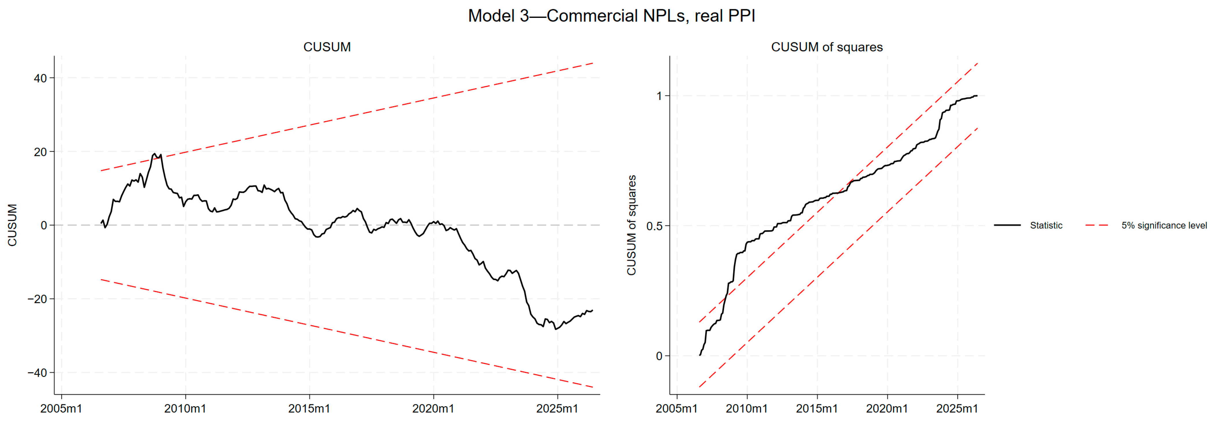
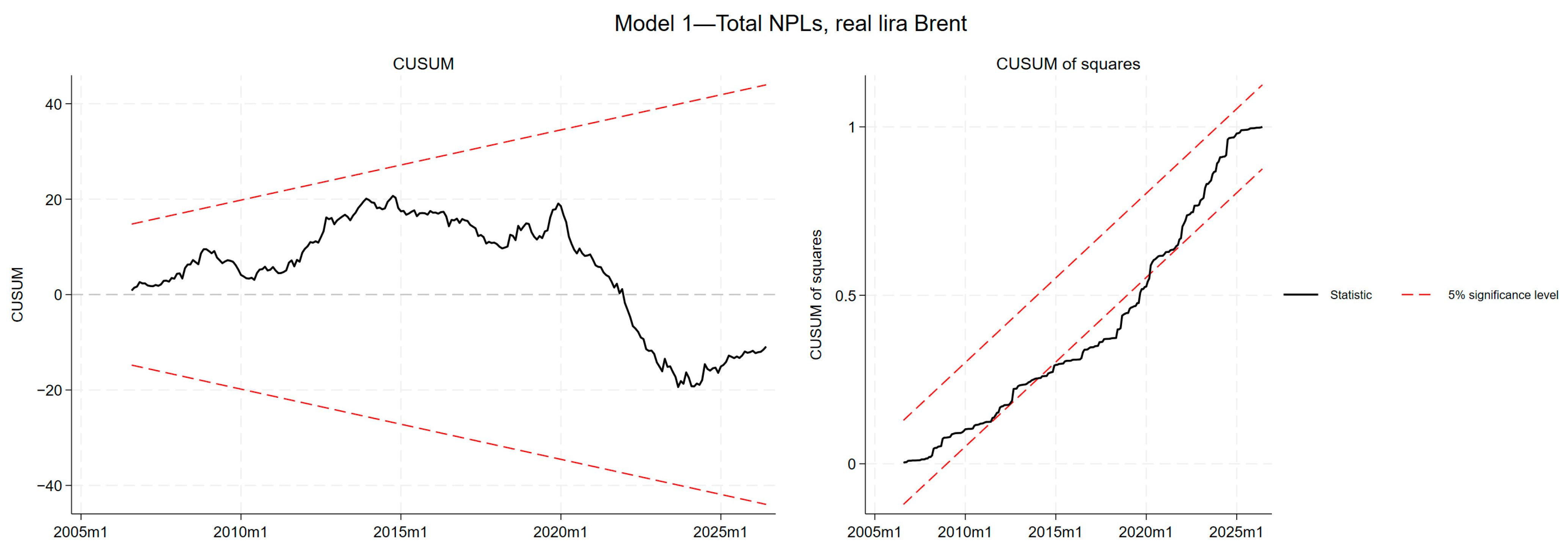
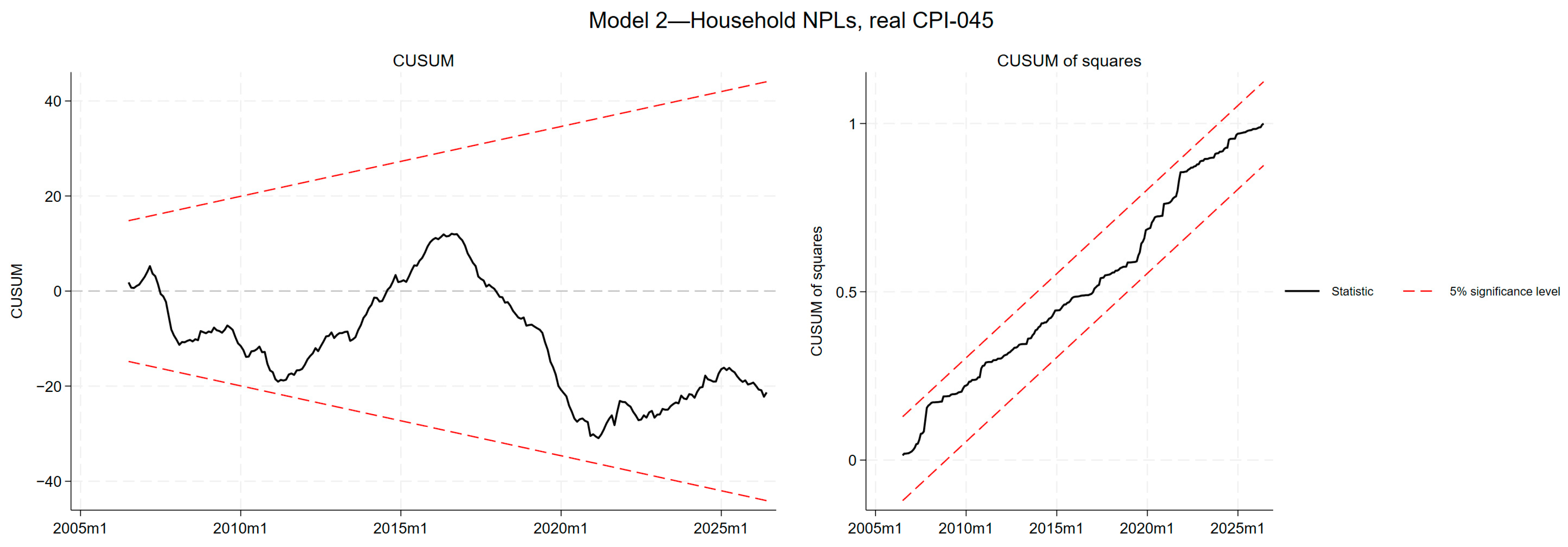
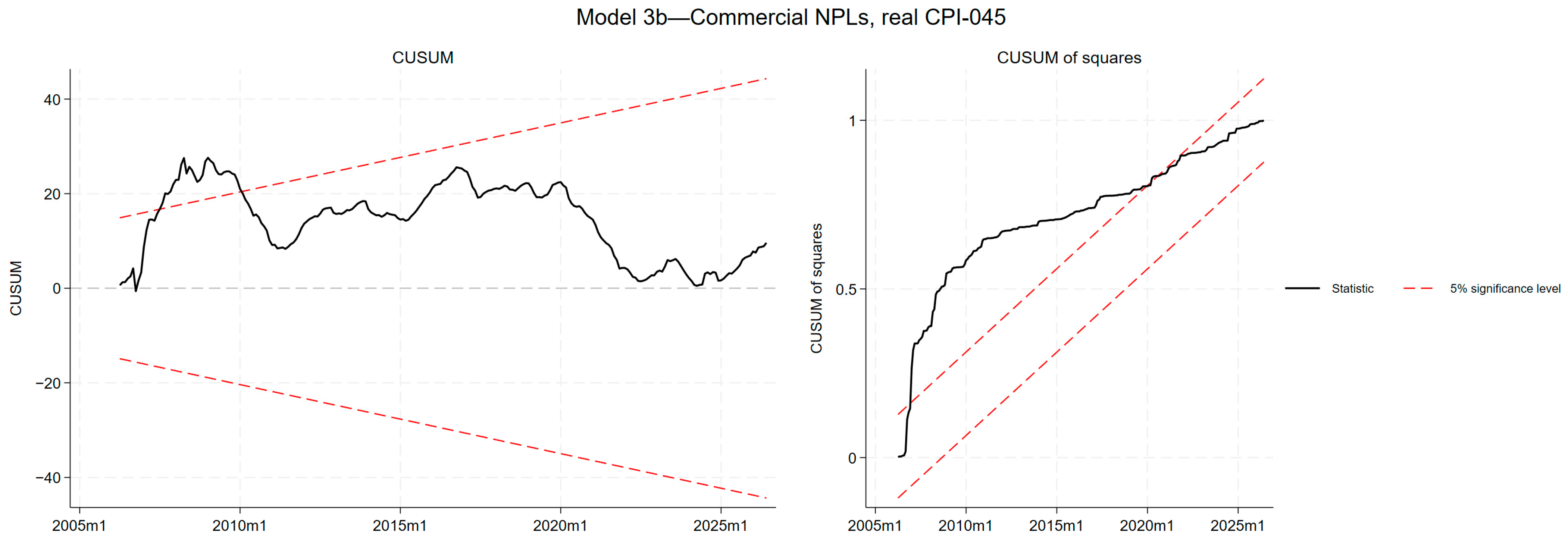
Autocorrelation was tested with the Breusch–Godfrey LM test, which remains valid in the presence of a lagged dependent variable, heteroskedasticity with the Breusch–Pagan test and functional form with the Ramsey RESET test (Ramsey, 1969); no conclusion in this paper rests on a result that only the first of the three inference procedures described above supports. Coefficient stability was examined with the CUSUM and CUSUM-of-squares tests of Brown et al. (1975).

4. Results

4.1. Unit Root and Cointegration Tests

Unit root tests for every series entering the models, including the positive and negative partial sums of the three relative energy indicators, are reported in Appendix A Table A3 (Augmented Dickey–Fuller in levels, Augmented Dickey–Fuller and Phillips–Perron in first differences). Every series except the industrial production index, which is stationary in levels, fails to reject a unit root in levels and rejects it at the 1 per cent level in first differences on both tests, so no series is integrated of order two; that, rather than a common order of integration, is the precondition for the bounds testing approach, whose asymptotic distribution is derived for a mixture of I(0) and I(1) regressors (Pesaran et al., 2001).

The existence of a long-run relationship was assessed in two stages, reported in Table 3. The asymptotic bounds test of Pesaran et al. (2001), computed with the finite-sample critical values of Kripfganz and Schneider (2020), places the F-statistic above the I(1) upper bound at the 1 per cent level in every model while the ECM t-statistics do not reach the I(1) bound in any model and do not even reach the I(0) bound in Models 1 and 3 at the 5 per cent level, so the joint decision rule returns no rejection for those two and an inconclusive verdict for Models 2 and 3b.

The asymptotic verdict was therefore supplemented with the bootstrap procedure of McNown et al. (2018) described in Section 3.4, computed on the same specification as Panel A of Table 3 with 1999 replications; the i.i.d. residual resampling of the original was run alongside the wild bootstrap and is reported where the two differ.

The overall F-statistic rejects at the 1 per cent level in every model, and the F-statistic on the regressors at the 1 per cent level in Models 2 and 3b and at the 5 per cent level in Models 1 and 3, so the verdict turns in each case on the t-test on the lagged dependent variable. In the commercial model estimated against the real consumer energy price, the three statistics reject jointly at the 10 per cent level (bootstrap p = 0.065 for the t-statistic under either resampling scheme) but not at the 5 per cent level. In the household model, the t-statistic does not reach the 10 per cent critical value of the wild bootstrap (p = 0.27) and clears it only under i.i.d. resampling (p = 0.07); the difference arises because the household residuals are markedly more volatile in the first year of the sample than thereafter, a pattern the wild bootstrap preserves and i.i.d. resampling removes, and the asymptotic verdict for this model is likewise inconclusive (Panel A). These are the two models from which the paper’s findings are drawn. In the total credit risk model and in the commercial model estimated against the real producer energy price, the overall F-statistic and the test on the regressors reject but the t-statistic on the lagged dependent variable does not, which is the second degenerate case: the regressors carry a level relationship among themselves that the dependent variable does not share. Evidence of a level relationship is therefore of the same kind in the two models that produce findings—strong from the two F-statistics, weak from the t-statistic—and it reaches the 10 per cent level only for the commercial model; for the two models that produce no findings it is absent. The long-run elasticities of Table 4 are accordingly reported conditional on a level relationship, inference from Models 1 and 3 is treated as descriptive throughout, and no claim in Section 5 rests on the level relationship alone. The symmetry restriction on which the paper’s findings turn is tested both on the long-run elasticities (L⁺ = L⁻, Section 4.3) and directly on the coefficients of the two partial sums in the error correction form (θ⁺ = θ⁻, Appendix B 

Table A5. Subsidiary robustness checks.

Specification	Model 1	Model 2	Model 3	Model 3b
A. +monetary tightening dummy (2023:M6–2024:M6)
Dummy p-value	0.011 **	0.609	0.000 ***	0.027 **
Energy symmetry Wald p	0.924	0.011 **	0.181	0.006 ***
Bounds test F	6.606	8.071	7.961	8.337
B. Symmetric lag augmentation
p = 1	0.156	0.004 ***	0.978	0.026 **
p = 2	0.166	0.002 ***	0.894	0.032 **
p = 3	0.311	0.036 **	0.811	0.027 **
p = 4	0.311	0.024 **	0.596	0.029 **
p = 6	0.238	0.082 *	0.439	0.081 *
C. Seasonality of the industrial production index
Raw index (as in the baseline)	0.829	0.001 ***	0.896	0.027 **
Deterministically deseasonalised index	0.989	0.000 ***	0.965	0.081 *
Raw index plus eleven monthly dummies	0.981	0.000 ***	0.905	0.067 *

Note: Cells report p-values of the ARDL Wald test of the null that the long-run responses to positive and negative energy price movements are equal, unless otherwise indicated; the baseline is Panel A of Table 9. Panel A adds a dummy for the monetary tightening of 2023:M6–2024:M6, which does not appear in the main specification. Panel B gives p lags to the dependent difference and to both energy differences simultaneously, holding the level block fixed; the corresponding Newey–West p-values range from 0.112 to 0.270 for Model 1, 0.014 to 0.054 for Model 2, 0.400 to 0.976 for Model 3 and 0.025 to 0.080 for Model 3b. Panels B and C report the Wald statistic computed on the level-block coefficients, so the first row of Panel C is the baseline under that same test and each column of the panel is internally comparable. The HAC and bootstrap versions of the symmetry test are in Panel A of Table 6 and Appendix A Table A1. *** p < 0.01, ** p < 0.05, and * p < 0.10.

), a test that does not presuppose a level relationship; the two are not numerically identical, since one restriction is linear and the other a ratio, but they agree in verdict in every case (Section 4.3), and the short-run dynamics of Section 4.4 point in the same direction.

Table 3. Bounds test results and the error correction term.

	Model 1 (Total × Real Brent)	Model 2 (Household × Real CPI-045)	Model 3 (Commercial × Real PPI)	Model 3b (Commercial × Real CPI-045)
Panel A. Asymptotic bounds test (Kripfganz–Schneider)
F-statistic	5.834	8.776	5.909	8.534
t-statistic	−1.939	−3.899	−2.678	−3.678
Joint decision	No rejection	Inconclusive	No rejection	Inconclusive
Panel B. Bootstrap bounds test (McNown–Sam–Goh, 1999 replications, same equation as Panel A)
Foverall	5.834	8.776	5.909	8.534
—bootstrap p	0.001 ***	0.002 ***	0.000 ***	0.000 ***
—bootstrap 10%|5% critical value	3.16|3.52	4.58|5.34	2.34|2.56	2.41|2.74
tdependent	−1.939	−3.899	−2.678	−3.678
—bootstrap p	0.697	0.272	0.188	0.065 *
—bootstrap 10%|5% critical value	−3.86|−4.22	−4.72|−5.29	−3.03|−3.30	−3.48|−3.76
—bootstrap p, i.i.d. resampling	0.634	0.072 *	0.221	0.066 *
Findependent	4.332	8.598	3.005	6.541
—bootstrap p	0.018 **	0.002 ***	0.013 **	0.000 ***
—bootstrap 10%|5% critical value	3.19|3.69	4.45|5.38	2.27|2.54	2.27|2.59
MSG verdict at 10%	Degenerate case 2	Degenerate case 2	Degenerate case 2	Cointegration
MSG verdict at 5%	Degenerate case 2	Degenerate case 2	Degenerate case 2	Degenerate case 2
Panel C. Error correction term
ECT	−0.018 *	−0.039 ***	−0.031 ***	−0.048 ***
ECT p-value	0.054	<0.001	0.008	<0.001
Implied half-life (months)	38.4	17.5	22.4	14.1
Observations	256	256	256	256

Note: Panel A reports the Pesaran et al. (2001) bounds test computed on the ARDL specification selected by the Akaike Information Criterion, with the finite-sample critical values and approximate p-values of Kripfganz and Schneider (2020) (k = 7, counting each partial sum as a separate regressor, N = 256; unrestricted intercept, no trend); the joint decision rule requires both the F- and the t-statistic to be more extreme than the I(1) values. Panel B reports the bootstrap procedure of McNown et al. (2018), computed on the same conditional error correction model as Panel A—identical sample, AIC-selected lag orders, intercept and crisis dummies—so that the three statistics, the long-run elasticities of Table 4 and the adjustment coefficients of Panel C are all drawn from one equation; the F- and t-statistics of the two panels therefore coincide. Bootstrap p-values and critical values are computed from 1999 replications generated under the null of no level relationship as described in Section 3.4; the row labelled i.i.d. resampling repeats the binding statistic under the residual resampling of McNown et al. (2018). The two schemes differ only in Model 2, whose residuals are markedly more volatile in the first year of the sample than thereafter; the wild bootstrap preserves that pattern and is the one on which the verdict is based. F(overall) tests that all lagged levels are jointly zero, t(dependent) the lagged level of the dependent variable, and F(independent) the lagged levels of the regressors jointly; only when all three reject can the degenerate cases be excluded, and “degenerate case 2” denotes rejection by the two F-statistics but not by t(dependent). In the terminology of McNown et al. (2018), degenerate case 2 is itself a verdict of no cointegration; the label is retained because it identifies which of the three statistics fails. Panel C reports the adjustment coefficient from the same specification; a significant adjustment coefficient is reported for completeness and is not itself a test of the level relationship; half-lives are ln(0.5)/ln(1 + ECT). *** p < 0.01, ** p < 0.05, and * p < 0.10.

Table 3. Bounds test results and the error correction term.

	Model 1 (Total × Real Brent)	Model 2 (Household × Real CPI-045)	Model 3 (Commercial × Real PPI)	Model 3b (Commercial × Real CPI-045)
Panel A. Asymptotic bounds test (Kripfganz–Schneider)
F-statistic	5.834	8.776	5.909	8.534
t-statistic	−1.939	−3.899	−2.678	−3.678
Joint decision	No rejection	Inconclusive	No rejection	Inconclusive
Panel B. Bootstrap bounds test (McNown–Sam–Goh, 1999 replications, same equation as Panel A)
Foverall	5.834	8.776	5.909	8.534
—bootstrap p	0.001 ***	0.002 ***	0.000 ***	0.000 ***
—bootstrap 10%|5% critical value	3.16|3.52	4.58|5.34	2.34|2.56	2.41|2.74
tdependent	−1.939	−3.899	−2.678	−3.678
—bootstrap p	0.697	0.272	0.188	0.065 *
—bootstrap 10%|5% critical value	−3.86|−4.22	−4.72|−5.29	−3.03|−3.30	−3.48|−3.76
—bootstrap p, i.i.d. resampling	0.634	0.072 *	0.221	0.066 *
Findependent	4.332	8.598	3.005	6.541
—bootstrap p	0.018 **	0.002 ***	0.013 **	0.000 ***
—bootstrap 10%|5% critical value	3.19|3.69	4.45|5.38	2.27|2.54	2.27|2.59
MSG verdict at 10%	Degenerate case 2	Degenerate case 2	Degenerate case 2	Cointegration
MSG verdict at 5%	Degenerate case 2	Degenerate case 2	Degenerate case 2	Degenerate case 2
Panel C. Error correction term
ECT	−0.018 *	−0.039 ***	−0.031 ***	−0.048 ***
ECT p-value	0.054	<0.001	0.008	<0.001
Implied half-life (months)	38.4	17.5	22.4	14.1
Observations	256	256	256	256

Note: Panel A reports the Pesaran et al. (2001) bounds test computed on the ARDL specification selected by the Akaike Information Criterion, with the finite-sample critical values and approximate p-values of Kripfganz and Schneider (2020) (k = 7, counting each partial sum as a separate regressor, N = 256; unrestricted intercept, no trend); the joint decision rule requires both the F- and the t-statistic to be more extreme than the I(1) values. Panel B reports the bootstrap procedure of McNown et al. (2018), computed on the same conditional error correction model as Panel A—identical sample, AIC-selected lag orders, intercept and crisis dummies—so that the three statistics, the long-run elasticities of Table 4 and the adjustment coefficients of Panel C are all drawn from one equation; the F- and t-statistics of the two panels therefore coincide. Bootstrap p-values and critical values are computed from 1999 replications generated under the null of no level relationship as described in Section 3.4; the row labelled i.i.d. resampling repeats the binding statistic under the residual resampling of McNown et al. (2018). The two schemes differ only in Model 2, whose residuals are markedly more volatile in the first year of the sample than thereafter; the wild bootstrap preserves that pattern and is the one on which the verdict is based. F(overall) tests that all lagged levels are jointly zero, t(dependent) the lagged level of the dependent variable, and F(independent) the lagged levels of the regressors jointly; only when all three reject can the degenerate cases be excluded, and “degenerate case 2” denotes rejection by the two F-statistics but not by t(dependent). In the terminology of McNown et al. (2018), degenerate case 2 is itself a verdict of no cointegration; the label is retained because it identifies which of the three statistics fails. Panel C reports the adjustment coefficient from the same specification; a significant adjustment coefficient is reported for completeness and is not itself a test of the level relationship; half-lives are ln(0.5)/ln(1 + ECT). *** p < 0.01, ** p < 0.05, and * p < 0.10.

4.2. Long-Run Coefficients

Table 4 reports the long-run elasticities, all energy indicators being in relative (real) terms (Section 3.1). Throughout Section 4 and Section 5, “raises” and “lowers” are used as shorthand for the sign of an estimated long-run conditional association; the design does not identify causal effects (see the fifth limitation in Section 6). The error correction term is negative in every model and significant at the 1 per cent level in three of the four, and the implied half-lives are long, indicating that non-performing loan ratios return to equilibrium slowly. Table 5 reports the cumulative dynamic multipliers that lie behind these elasticities; they are discussed in Section 4.4.

Table 4. Long-run coefficients (elasticities), conditional on a level relationship.

Variable	Model 1 Total × Real Brent	Model 2 Household × Real CPI-045	Model 3 Commercial × Real PPI	Model 3b Commercial × Real CPI-045
Energy price (+)	−0.824	+1.864 **	−0.860	+0.421
Energy price (−)	−0.700 **	−0.917	−0.282	+3.541 ***
FX volatility (+)	+0.249	+0.454 ***	+0.752 **	+0.563 ***
FX volatility (−)	+0.222	+0.558 ***	+0.669 *	+0.366 **
Policy rate	+0.563 *	+0.172	+0.625	+0.987 **
Real effective exchange rate	+2.443	+1.061 *	+4.603 **	+5.193 ***
Industrial production	+1.962	+1.026	+1.180	+0.341
Error correction term	−0.018 *	−0.039 ***	−0.031 ***	−0.048 ***
Selected ARDL order	(2, 0, 0, 1, 0, 0, 2, 2)	(2, 0, 0, 1, 0, 1, 0, 2)	(2, 0, 2, 1, 2, 0, 0, 0)	(2, 0, 0, 1, 0, 0, 0, 0)
Observations	256	256	256	256

Note: All energy indicators are relative (real), that is, the energy index divided by the corresponding general price index. Model 1 uses the real lira price of Brent crude, Models 2 and 3b the real CPI-045 consumer energy index, and Model 3 the real PPI energy index. Since all variables are in logarithms, the coefficients are interpreted as elasticities. The negative partial sum is a decreasing series, so a negative coefficient on it means that a price decline raises the ratio, and a positive coefficient means that a decline lowers it. *** p < 0.01, ** p < 0.05, and * p < 0.10.

Table 4. Long-run coefficients (elasticities), conditional on a level relationship.

Variable	Model 1 Total × Real Brent	Model 2 Household × Real CPI-045	Model 3 Commercial × Real PPI	Model 3b Commercial × Real CPI-045
Energy price (+)	−0.824	+1.864 **	−0.860	+0.421
Energy price (−)	−0.700 **	−0.917	−0.282	+3.541 ***
FX volatility (+)	+0.249	+0.454 ***	+0.752 **	+0.563 ***
FX volatility (−)	+0.222	+0.558 ***	+0.669 *	+0.366 **
Policy rate	+0.563 *	+0.172	+0.625	+0.987 **
Real effective exchange rate	+2.443	+1.061 *	+4.603 **	+5.193 ***
Industrial production	+1.962	+1.026	+1.180	+0.341
Error correction term	−0.018 *	−0.039 ***	−0.031 ***	−0.048 ***
Selected ARDL order	(2, 0, 0, 1, 0, 0, 2, 2)	(2, 0, 0, 1, 0, 1, 0, 2)	(2, 0, 2, 1, 2, 0, 0, 0)	(2, 0, 0, 1, 0, 0, 0, 0)
Observations	256	256	256	256

Note: All energy indicators are relative (real), that is, the energy index divided by the corresponding general price index. Model 1 uses the real lira price of Brent crude, Models 2 and 3b the real CPI-045 consumer energy index, and Model 3 the real PPI energy index. Since all variables are in logarithms, the coefficients are interpreted as elasticities. The negative partial sum is a decreasing series, so a negative coefficient on it means that a price decline raises the ratio, and a positive coefficient means that a decline lowers it. *** p < 0.01, ** p < 0.05, and * p < 0.10.

Table 5. Cumulative dynamic multipliers of the log NPL ratio (90% bootstrap bands).

Horizon	Model 2 Household × Real CPI-045: Increase	Model 2: Decrease	Model 3b Commercial × Real CPI-045: Increase	Model 3b: Decrease
1 month	0.15 [0.07, 0.28]	−0.07 [−0.14, 0.02]	0.03 [−0.08, 0.13]	0.29 [0.22, 0.42]
6 months	0.50 [0.22, 0.85]	−0.25 [−0.44, 0.06]	0.10 [−0.24, 0.38]	0.86 [0.67, 1.21]
12 months	0.83 [0.34, 1.32]	−0.41 [−0.71, 0.09]	0.17 [−0.39, 0.62]	1.42 [1.09, 1.91]
24 months	1.27 [0.50, 1.86]	−0.62 [−1.05, 0.13]	0.26 [−0.56, 0.92]	2.21 [1.61, 2.84]
Long run (Table 4)	1.86	−0.92	0.42	3.54
Equality of the two multipliers, percentile p	<0.001 at every horizon		<0.001 at every horizon

Note: Multipliers are the cumulative responses of the log NPL ratio to a unit change in the cumulated partial sum after h months, computed recursively from the level-form ARDL coefficients of Table 4 specifications (the same lag orders, sample and dummies); unlike the long-run elasticities, they do not presuppose a level relationship. Bands are 5th–95th percentiles of 999 Rademacher residual-bootstrap replications of the level ARDL; the equality p-value is the two-sided percentile p of the bootstrap difference between the two multipliers.

Table 5. Cumulative dynamic multipliers of the log NPL ratio (90% bootstrap bands).

Horizon	Model 2 Household × Real CPI-045: Increase	Model 2: Decrease	Model 3b Commercial × Real CPI-045: Increase	Model 3b: Decrease
1 month	0.15 [0.07, 0.28]	−0.07 [−0.14, 0.02]	0.03 [−0.08, 0.13]	0.29 [0.22, 0.42]
6 months	0.50 [0.22, 0.85]	−0.25 [−0.44, 0.06]	0.10 [−0.24, 0.38]	0.86 [0.67, 1.21]
12 months	0.83 [0.34, 1.32]	−0.41 [−0.71, 0.09]	0.17 [−0.39, 0.62]	1.42 [1.09, 1.91]
24 months	1.27 [0.50, 1.86]	−0.62 [−1.05, 0.13]	0.26 [−0.56, 0.92]	2.21 [1.61, 2.84]
Long run (Table 4)	1.86	−0.92	0.42	3.54
Equality of the two multipliers, percentile p	<0.001 at every horizon		<0.001 at every horizon

Note: Multipliers are the cumulative responses of the log NPL ratio to a unit change in the cumulated partial sum after h months, computed recursively from the level-form ARDL coefficients of Table 4 specifications (the same lag orders, sample and dummies); unlike the long-run elasticities, they do not presuppose a level relationship. Bands are 5th–95th percentiles of 999 Rademacher residual-bootstrap replications of the level ARDL; the equality p-value is the two-sided percentile p of the bootstrap difference between the two multipliers.

The long-run energy coefficients differ sharply across borrower types, and the direction of the difference is the study’s central result. In the household model, a 1 per cent cumulative increase in the real consumer energy price is associated with a 1.86 per cent higher household non-performing loan ratio in the long run, while the coefficient on the negative partial sum is insignificant: declines in the real consumer energy price do not lower the household ratio, and if anything, the point estimate goes the other way.

The commercial portfolio displays the mirror image, but only when it is confronted with the same consumer energy price (Model 3b). There, the coefficient on the positive partial sum is small and insignificant, whereas the coefficient on the negative partial sum is +3.54 and significant at the 1 per cent level, so a 1 per cent fall in the real consumer energy price is associated with a commercial non-performing loan ratio about 3.5 per cent lower in the long run, while increases are associated with no change. Firms, in other words, obtain relief from a falling real consumer energy price that households do not; Section 5.1 traces where that relief comes from.

The economic magnitude of these elasticities can be gauged against the shocks actually observed. Over the sample, the positive partial sum of the real consumer energy price grows by 0.12 log points in an average calendar year (median 0.06), by 0.27–0.42 in the shock years 2022–2024, and by at most 0.56 over any twelve-month window (to August 2024). With a long-run elasticity of 1.86, a typical year of real increases—taken here as 10 per cent, a round figure between the mean and the median of the annual changes just reported—is associated with a household non-performing loan ratio about 19 per cent higher in the long run: from its sample mean of 3.44 per cent to 4.08 per cent, or 0.6 percentage points, roughly two-thirds of the series’ standard deviation (1.0 point); at the household loan stock of mid-2026, about TL 7.0 trillion, 0.6 points corresponds to roughly TL 45 billion of additional non-performing receivables. A year of the 2022–2024 kind (27–42 per cent) is associated with a ratio 1.7–2.7 points higher, and the largest twelve-month increase in the sample with a ratio roughly twice its mean; since the adjustment half-life is 17 months, only about two-fifths of any such long-run association materialises within the first year, and the largest figure should be read as an upper bound rather than a forecast. These are long-run associations conditional on the level relationship discussed in Section 4.1.

On the commercial side, the negative partial sum falls by 0.12 log points in an average year (median 0.07), the distribution being dominated by 2023, when a single administrative decision in May accounted for 0.45 of that year’s 0.82 decline; with an elasticity of 3.54, a typical year of real declines—taken as 5–10 per cent, a range spanning the median annual decline—is associated with a commercial ratio 18–35 per cent lower in the long run, or 0.7 to 1.4 percentage points from a mean of 4.0, which is why the May 2023 episode is controlled for separately in Section 4.6. For comparison, the real effective exchange rate, the most consistent control, has a twelve-month log change with a standard deviation of 0.105 and long-run elasticities of 1.06 and 5.19 in the household and commercial equations: a one-standard-deviation real appreciation is associated with a household ratio 11 per cent higher and a commercial ratio 55 per cent higher. An energy price shock of typical size is therefore of the same order as an exchange rate shock for the household portfolio and smaller than one for the commercial portfolio.

Neither the producer energy price nor the real lira price of crude produces a comparable pattern. In Model 3, where commercial credit risk is confronted with the real producer energy price, both energy coefficients are small and far from significance. In Model 1, the positive component of the real lira Brent price is insignificant while the negative component is significant at the 5 per cent level, but as Section 4.3 shows, the two are not statistically distinguishable from one another. The association between energy prices and credit risk therefore appears through what borrowers pay at the consumer level rather than through the cost of energy to producers or the world price of crude.

The producer-price results also discipline the reading of the earlier literature. Estimated on a nominal index, the producer energy price appeared to carry a negative long-run coefficient for commercial credit risk (−1.35, p = 0.10); once the index is expressed relative to the general producer price index, the coefficient loses both its magnitude and its significance (−0.86, p = 0.70). The nominal result was capturing the inflation trend common to the numerator and the denominator of the ratio rather than an energy-specific effect, which is the principal reason the relative specification is adopted throughout.

Among the control variables, the real effective exchange rate produces the most consistent effect, entering positively in every model and significantly in three of the four. Since an increase in the index corresponds to a real appreciation of the Turkish lira, credit risk accumulates during phases of real appreciation; a relationship in the same direction was reported by Castro (2013) for the GIPSI countries, and Section 5.3 takes up the interpretation. Exchange rate volatility also enters positively in every model, and in the commercial equation estimated against the consumer energy price, its effect is itself asymmetric, the null of equal responses to volatility increases and decreases being rejected at the 1 per cent level against the 10 per cent level for households and not at all elsewhere.

4.3. Asymmetry Tests and the Cross-Portfolio Comparison

Table 6 reports the Wald tests of the null that the long-run responses to positive and negative energy price movements are equal. Panel A applies the three inference procedures of Section 3.4 to each model, and the three agree. Symmetry is rejected in the household model and in the commercial model estimated against the consumer energy price, and cannot be rejected anywhere else—neither for total credit risk against the real lira price of crude nor for commercial credit risk against the producer energy price.

The two rejections point in opposite directions—for households the significant component is the positive one, for firms the negative one—and whether that difference is statistically established is the question taken up next.

Table 6. Wald tests of the long-run symmetry hypothesis.

Hypothesis/Method			Model 1 Total × Real Brent	Model 2 Household × Real CPI-045		Model 3 Commercial × Real PPI	Model 3b Commercial × Real CPI-045
Panel A. Baseline models, three inference procedures
Energy L+ = L−, ARDL Wald			0.839	0.009 ***		0.894	0.010 **
Energy L+ = L−, Newey–West HAC			0.823	0.014 **		0.886	0.000 ***
Energy L+ = L−, wild bootstrap (999)			0.816	0.004 ***		0.873	0.007 ***
FX volatility, L+ = L−			0.787	0.054 *		0.738	0.002 ***
Dependent Variable	Brent (USD)	Brent (TRY)	Brent (Real TRY)	CPI-045 (Nominal)	CPI-045 (Real)	PPI Energy (Nominal)	PPI Energy (Real)
Panel B. Symmetry Wald p-values across all loan–indicator combinations
Total NPL	0.838	0.401	0.839	0.253	0.797	0.102	0.508
—FDR adjusted	0.894	0.702	0.894	0.532	0.894	0.267	0.820
Household NPL	0.024 **	0.004 ***	0.002 ***	0.032 **	0.009 ***	0.592	0.242
—FDR adjusted	0.082 *	0.026 **	0.024 **	0.097*	0.043 **	0.887	0.532
Commercial NPL	0.879	0.780	0.705	0.001 ***	0.010 **	0.361	0.894
—FDR adjusted	0.894	0.894	0.894	0.024 **	0.043 **	0.689	0.894

Note: The cells report p-values of the Wald test of the null that the long-run responses to positive and negative energy price movements are equal; the final row of Panel A applies the same test to exchange rate volatility. The restriction is tested on the long-run elasticities L = −θ/ρ by the delta method; the equivalent restriction on the error-correction coefficients (θ⁺ = θ⁻) is reported in Appendix B Table A5. Panel A applies three inference procedures to the four baseline models, all computed on the same equation as the long-run coefficients in Table 4, so that the point estimates are identical across them and only the covariance matrix changes. Panel B holds the specification fixed and varies only the dependent variable and the energy indicator, so that a property of the borrower can be separated from a property of the price series; each cell comes from an ARDL(2,·) model selected by AIC with the same controls and crisis dummies as the baseline. Because Panel B comprises twenty-one simultaneous tests, Benjamini–Hochberg adjusted p-values controlling the false discovery rate are reported beneath each row; five cells survive adjustment at the 5 per cent level, including both of the pairings that appear as baseline models in Panel A, and two survive the stricter Holm correction. Panel B is exploratory in purpose: the confirmatory tests are those of Panel A, which are pre-specified rather than selected from a grid. *** p < 0.01, ** p < 0.05, and * p < 0.10.

Table 6. Wald tests of the long-run symmetry hypothesis.

Hypothesis/Method			Model 1 Total × Real Brent	Model 2 Household × Real CPI-045		Model 3 Commercial × Real PPI	Model 3b Commercial × Real CPI-045
Panel A. Baseline models, three inference procedures
Energy L+ = L−, ARDL Wald			0.839	0.009 ***		0.894	0.010 **
Energy L+ = L−, Newey–West HAC			0.823	0.014 **		0.886	0.000 ***
Energy L+ = L−, wild bootstrap (999)			0.816	0.004 ***		0.873	0.007 ***
FX volatility, L+ = L−			0.787	0.054 *		0.738	0.002 ***
Dependent Variable	Brent (USD)	Brent (TRY)	Brent (Real TRY)	CPI-045 (Nominal)	CPI-045 (Real)	PPI Energy (Nominal)	PPI Energy (Real)
Panel B. Symmetry Wald p-values across all loan–indicator combinations
Total NPL	0.838	0.401	0.839	0.253	0.797	0.102	0.508
—FDR adjusted	0.894	0.702	0.894	0.532	0.894	0.267	0.820
Household NPL	0.024 **	0.004 ***	0.002 ***	0.032 **	0.009 ***	0.592	0.242
—FDR adjusted	0.082 *	0.026 **	0.024 **	0.097*	0.043 **	0.887	0.532
Commercial NPL	0.879	0.780	0.705	0.001 ***	0.010 **	0.361	0.894
—FDR adjusted	0.894	0.894	0.894	0.024 **	0.043 **	0.689	0.894

Note: The cells report p-values of the Wald test of the null that the long-run responses to positive and negative energy price movements are equal; the final row of Panel A applies the same test to exchange rate volatility. The restriction is tested on the long-run elasticities L = −θ/ρ by the delta method; the equivalent restriction on the error-correction coefficients (θ⁺ = θ⁻) is reported in Appendix B Table A5. Panel A applies three inference procedures to the four baseline models, all computed on the same equation as the long-run coefficients in Table 4, so that the point estimates are identical across them and only the covariance matrix changes. Panel B holds the specification fixed and varies only the dependent variable and the energy indicator, so that a property of the borrower can be separated from a property of the price series; each cell comes from an ARDL(2,·) model selected by AIC with the same controls and crisis dummies as the baseline. Because Panel B comprises twenty-one simultaneous tests, Benjamini–Hochberg adjusted p-values controlling the false discovery rate are reported beneath each row; five cells survive adjustment at the 5 per cent level, including both of the pairings that appear as baseline models in Panel A, and two survive the stricter Holm correction. Panel B is exploratory in purpose: the confirmatory tests are those of Panel A, which are pre-specified rather than selected from a grid. *** p < 0.01, ** p < 0.05, and * p < 0.10.

A separate question is whether these results are a property of the borrower or of the particular price series used. Panel B of Table 6 therefore reports every combination of the three loan portfolios with seven energy indicators. The household row rejects symmetry against five of the seven, and the rejection strengthens as the indicator moves closer to what households actually pay, from dollar Brent to lira Brent to real lira Brent. The commercial row rejects only against the consumer energy index, in both its nominal and its real form. Neither portfolio responds asymmetrically to the producer energy price, and total credit risk responds asymmetrically to nothing. The asymmetry is therefore attached to the borrower and to consumer-level energy prices jointly, and it is not an artefact of the CPI-045 series, since it also appears against crude oil once that price is expressed in the currency and at the price level households face. The grid is exploratory (see the note to Table 6); the confirmatory tests are those of Panel A.

The household and commercial equations were then estimated as a seemingly unrelated regression system on a common sample, with both confronted with the same energy indicator—the real consumer energy price—so that the borrower is the only thing that varies.

Table 7. Cross-equation tests of borrower-specific asymmetry.

Test		Statistic		p-Value
Panel A. System A: household vs. commercial, both on the real consumer energy price (AIC-selected lag orders, N = 256)
Household equation, L+ = L−		χ2(1) = 7.70		0.006 ***
Commercial equation, L+ = L−		χ2(1) = 5.83		0.016 **
Cross-equation: (L+ − L−)hh = (L+ − L−)cm		χ2(1) = 14.17		<0.001 ***
Household asymmetry gap, L+ − L−		+2.663 (0.960)		0.006 ***
Commercial asymmetry gap, L+ − L−		−3.166 (1.311)		0.016 **
Difference between the two gaps		+5.829 (1.548)		<0.001 ***
Block bootstrap of the difference, bootstrap-t p (12-month blocks, 1999 replications)				0.007 ***
Block bootstrap, 95% bootstrap-t interval/percentile interval		[3.84, 10.13]/[0.29, 12.97]
Block length 6/24 months, bootstrap-t p				0.0005 ***/0.021 **
Equality of the raw coefficient gaps, θ+ − θ− (no ratio)		+0.244 (0.069)		<0.001 *** (bootstrap-t 0.005 ***)
Equality of the adjustment speeds, ρhh = ρcm		−0.040 vs. −0.043		0.870
Specification	Household Gap L+ − L− (s.e.)	Commercial Gap L+ − L− (s.e.)	Difference (s.e.)	Asymptotic p	Bootstrap-t p
Panel B. Cross-equation restriction under alternative specifications (same energy indicator; 12-month-block bootstrap)
Fixed lag structure (one lagged difference), N = 256	+1.992 (0.810)	−3.611 (1.416)	+5.603 (1.543)	<0.001 ***	0.013 **
AIC-selected lag orders (Panel A)	+2.663 (0.960)	−3.166 (1.311)	+5.829 (1.548)	<0.001 ***	0.007 ***
AIC orders selected with a maximum of three lags	+2.745 (0.894)	−3.131 (1.303)	+5.877 (1.498)	<0.001 ***	0.006 ***
Seasonally adjusted industrial production	+3.343 (1.107)	−2.654 (1.618)	+5.998 (1.860)	0.001 ***	0.002 ***
COVID-19 dummy added	+1.931 (0.865)	−3.420 (1.444)	+5.351 (1.603)	<0.001 ***	0.019 **
Both equations in level form (percentage points)	+8.263 (3.352)	−8.272 (6.749)	+16.535 (7.028)	0.019 **	0.019 **
May 2023 removed from the partial sums (AIC lag orders)	+3.122 (1.067)	−6.562 (2.370)	+9.684 (2.501)	<0.001 ***	0.008 ***

Note: Seemingly unrelated regression systems estimated on a common sample of 256 observations (255 where three lags are allowed) with the same controls and crisis dummies as the baseline models; in Panel A, each equation carries the lag orders selected for it by the AIC (Table 4), so that Table 4 and Table 7 describe the same equations. In every system, the two equations are confronted with the same energy indicator, the real consumer energy price, so that borrower type is the only source of variation and the cross-equation restriction isolates it. L⁺ and L⁻ denote the long-run elasticities −θ⁺/ρ and −θ⁻/ρ, and every test in the table except the equality of the adjustment speeds and the row on the raw coefficient gaps is computed on those elasticities by the delta method rather than on the raw coefficients; the discussion below explains why the distinction matters. Standard errors are in parentheses. The implied long-run elasticities in System A are +1.803 and −0.860 for households and +0.571 and +3.737 for firms, for positive and negative movements, respectively. The block bootstrap is the row-block bootstrap of the two-equation system described in Section 3.4; the bootstrap-t interval and p-value come from the same 1999 replications (none failed), the percentile interval is shown for comparison only, and block lengths of 6 and 24 months are reported for sensitivity. Panel B repeats the test under the alternative specifications of Section 4.6 and reports the two asymmetry gaps, their difference, the asymptotic p-value of the equality restriction and the bootstrap-t p-value with twelve-month blocks (1999 replications for the fixed-lag, AIC and May 2023 systems, 999 otherwise); in the level-form system, the gaps are in percentage points, and the commercial equation does not itself reject symmetry (p = 0.22), yet the difference between the two gaps still does. The May 2023 row removes the natural gas subsidy from the cumulated partial sums. *** p < 0.01 and ** p < 0.05.

reports the results.

Within the system, both equations reject symmetry in their long-run elasticities. The estimated asymmetry gaps carry opposite signs, positive for households and negative for firms, and the restriction that the two are equal is rejected at well below the 1 per cent level by the asymptotic test (bootstrap inference is reported below). The test is computed on the long-run elasticities −θ/ρ rather than on the raw coefficients θ, since it is the long-run responses, not the short-run coefficients, that the comparison concerns. The distinction is not merely formal: a test on the raw coefficients would be valid only if the two portfolios adjusted at the same speed. In this system, they very nearly do, and their equality cannot be rejected, so the two versions of the test happen to agree; but only the elasticity version tests the restriction the paper asserts.

Two further checks indicate that the result is not an artefact of a single episode or of the asymptotic distribution of the test. First, the same system was re-estimated with the May 2023 natural gas subsidy removed from the cumulated partial sums; both equations continue to reject symmetry, the cross-equation restriction is still rejected at the 1 per cent level, and the difference between the two gaps widens (Table 7, Panel B; bootstrap-t p = 0.008). Second, the sampling distribution of the studentised difference was obtained by a moving-block bootstrap of the system (Section 3.4): the bootstrap-t p-value is 0.007 with twelve-month blocks, 0.0005 with six-month blocks and 0.021 with twenty-four-month blocks, and the bootstrap-t 95 per cent interval, [3.8, 10.1], excludes zero (Table 7). The bootstrap is the more conservative of the two forms of inference, as is to be expected of one that makes no distributional assumption: the asymptotic test rejects at well below the 1 per cent level, the bootstrap at the 1 per cent level with the baseline block length and at the 5 per cent level with the longest, and the sign of the difference is the same throughout. A test on the raw coefficient gaps, which involves no ratio, rejects at the 1 per cent level under both forms of inference.

Two qualifications attach to the firm side of this comparison rather than to the household side: the commercial equations are diagnostically the weaker ones (Section 4.5), and re-estimating them in level form or seasonally adjusting industrial production preserves the sign pattern but not the within-equation rejection of symmetry (Section 4.6 and Appendix B Table A5, Panel C). The cross-equation result should therefore be read as establishing that the two portfolios respond differently—the difference between the two gaps keeps its sign and rejects equality, asymptotically and under the block bootstrap, in every specification of Table 7, Panel B, including the level-form system in which the commercial equation on its own no longer rejects symmetry—rather than as a precise estimate of the firm-side elasticity.

4.4. Short-Run Dynamics

Table 8. Short-run coefficients.

Term	Model 1 Total × Real Brent	Model 2 Household × Real CPI-045	Model 3 Commercial × Real PPI	Model 3b Commercial × Real CPI-045
ΔNPL(−1)	+0.221 (0.000)	+0.124 (0.037)	−0.220 (0.000)	−0.249 (0.000)
ΔEnergy(−)	—	—	−0.406 (0.057)	—
ΔEnergy(−)(−1)	—	—	+0.745 (0.001)	—
ΔFX volatility(+)	−0.018 (0.000)	−0.028 (0.000)	−0.038 (0.006)	−0.031 (0.015)
ΔFX volatility(−)	—	—	+0.010 (0.508)	—
ΔFX volatility(−)(−1)	—	—	−0.023 (0.078)	—
ΔPolicy rate	—	−0.038 (0.070)	—	—
ΔREER	+0.256 (0.000)	—	—	—
ΔREER(−1)	−0.262 (0.000)	—	—	—
ΔIPI	−0.027 (0.175)	−0.124 (0.000)	—	—
ΔIPI(−1)	−0.034 (0.037)	−0.070 (0.001)	—	—
d_2018	+0.031 (0.000)	+0.017 (0.136)	+0.061 (0.008)	+0.046 (0.040)
d_gfc	+0.037 (0.000)	+0.045 (0.000)	+0.098 (0.000)	+0.108 (0.000)
Constant	−0.361 (0.037)	−0.312 (0.067)	−0.856 (0.009)	−1.434 (0.000)
Error correction term (ECT)	−0.018 (0.054)	−0.039 (0.000)	−0.031 (0.008)	−0.048 (0.000)

Note: Coefficients with p-values in parentheses. Only the terms retained by the AIC lag selection appear in each column; a dash indicates that the term is not part of that model’s selected specification. Δ denotes the first difference and (−1) a one-period lag. The dummy variables d_2018 and d_gfc mark the August 2018 currency shock (2018:M8–2019:M6) and the global financial crisis (2008:M9–2009:M12), respectively.

reports the short-run error correction dynamics. Three regularities hold across the models. First, the lagged change in the non-performing loan ratio is significant in every equation, positively for the total and household portfolios and negatively for the two commercial specifications, so the commercial series overshoots and partially reverses within a month. Second, positive shocks to exchange rate volatility carry a significant negative short-run coefficient everywhere while their long-run coefficient is positive: volatility shocks are associated with a brief fall in delinquency and a rise thereafter. Third, industrial production enters the household equation with a strongly negative contemporaneous and lagged effect, which is the expected employment channel; the same channel is visible but far weaker in the total portfolio, where only the lagged term is significant, and it is absent from both commercial equations. In the commercial model, the short-run coefficients on the real producer energy price change sign between the contemporaneous and the lagged term, consistent with whatever transmission exists on the producer side being short-lived and not accumulating into a long-run relationship.

The short-run coefficients describe the impact month only. Table 5 traces the cumulative response over six, twelve and twenty-four months, which requires no assumption about the level relationship: after twelve months, the household ratio has moved by 0.83 log points per unit increase in the cumulated real consumer energy price (90% band 0.34 to 1.32) and by −0.41 per unit decrease (−0.71 to 0.09), and the two multipliers differ at every horizon; the commercial pattern is the mirror image, 0.17 (−0.39 to 0.62) for increases and 1.42 (1.09 to 1.91) for decreases. Roughly two-fifths of the long-run association is thus in place within a year, and the direction-dependence that the long-run elasticities display is already visible at the medium-term horizon.

4.5. Diagnostic Tests and Parameter Stability

The statistical validity of the estimated models was assessed with the battery of tests reported in Appendix A 

Table A4. Residual diagnostics and CUSUM/CUSUM-of-squares results.

Test	Model 1 Total × Real Brent	Model 2 Household × Real CPI-045	Model 3 Commercial × Real PPI	Model 3b Commercial × Real CPI-045
Observations	256	256	256	256
R2/adjusted R2	0.534/0.503	0.426/0.390	0.294/0.247	0.279/0.244
Breusch–Godfrey LM (1 lag)	0.271	0.193	0.487	0.672
Breusch–Godfrey LM (2 lags)	0.334	0.032	0.192	0.306
Breusch–Godfrey LM (4 lags)	0.106	0.035	0.046	0.557
Breusch–Pagan heteroskedasticity	0.890	0.695	0.000	0.000
Ramsey RESET	0.792	0.638	0.000	0.000
Skewness–kurtosis normality	0.004	0.000	0.000	0.000
CUSUM	Within bounds	Within bounds	Outside 5 months, 2008:M9–2009:M1	Outside 31 months, 2007:M7–2010:M1
CUSUMSQ	Below lower band, 74 months, 2014:M2–2020:M3	Within bounds	Above upper band, 96 months, 2008:M7–2016:M6	Above upper band, 160 months, 2007:M1–2020:M7

Note: Cells report p-values except in the first two and the last two rows. All tests are computed on the conditional error correction model in the exact lag order selected by the Akaike Information Criterion, and in the timing that selection imposes: a regressor whose lag order is zero enters the level block contemporaneously rather than with a one-period lag. The CUSUM and CUSUM-of-squares rows report the months in which each statistic lies outside its 5 per cent significance band, computed from the recursive residuals of the same equation against the bands of Brown et al. (1975) and counted directly rather than read off the plots in Figure 1, Figure 2, Figure 3 and Figure 4; the number of recursive residuals available is 239, 240, 239 and 243 for the four models, respectively, the difference reflecting the number of parameters estimated in each. “Within bounds” means that the statistic does not leave its band in any month of the sample. Because serial correlation is present in Model 2 and marginally in Model 3, and heteroskedasticity in Models 3 and 3b, no inference reported in this paper relies on ordinary least squares standard errors.

, computed on the conditional error correction model in the exact lag order selected by AIC. The total and household models are well behaved on the Breusch–Pagan and Ramsey RESET tests. The household model, from which the study’s central finding is drawn, displays mild residual serial correlation, the Breusch–Godfrey test rejecting only at the second and fourth lags, so ordinary least squares standard errors are not relied upon for inference in that model: the asymmetry test is reported throughout in the three forms of Section 3.4, and the long-run elasticities and confidence intervals in Appendix A 

Table A1. Long-run coefficients with Newey–West HAC standard errors.

Variable	Model 1	Model 2	Model 3	Model 3b
Energy price (+)	−0.824 (0.303)	+1.864 (0.024) **	−0.860 (0.683)	+0.421 (0.714)
—95% CI	[−2.39, 0.74]	[0.25, 3.48]	[−4.99, 3.27]	[−1.83, 2.67]
Energy price (−)	−0.700 (0.073) *	−0.917 (0.115)	−0.282 (0.907)	+3.541 (0.003) ***
—95% CI	[−1.47, 0.07]	[−2.06, 0.22]	[−5.01, 4.44]	[1.17, 5.91]
FX volatility (+)	+0.249 (0.345)	+0.454 (0.000) ***	+0.752 (0.071) *	+0.563 (0.000) ***
FX volatility (−)	+0.222 (0.262)	+0.558 (0.000) ***	+0.669 (0.146)	+0.366 (0.010) **
Policy rate	+0.563 (0.167)	+0.172 (0.260)	+0.625 (0.444)	+0.987 (0.079) *
Real effective exchange rate	+2.443 (0.266)	+1.061 (0.160)	+4.603 (0.075) *	+5.193 (0.001) ***
Industrial production	+1.962 (0.389)	+1.026 (0.272)	+1.180 (0.443)	+0.341 (0.748)
Error correction term	−0.018 (0.137)	−0.039 (0.000) ***	−0.031 (0.051) *	−0.048 (0.005) ***
Energy symmetry Wald p	0.823	0.014 **	0.886	0.000 ***
Observations	256	256	256	256

Note: Each column reports the long-run elasticities of the model in the corresponding column of Table 4, computed as L = −θ/ρ by the delta method. The equation, the lag structure and the estimation sample are identical to those of Table 4; the point estimates are therefore identical by construction and only the standard errors, p-values and confidence intervals differ. Standard errors are those of Newey and West (1987) with four lags; p-values based on them are in parentheses. Confidence intervals are reported for the two energy coefficients, on which the study’s findings rest, and are available from the authors for the remaining coefficients. The symmetry test is the Wald test of L⁺ = L⁻ computed by the delta method on the same covariance matrix; it is stable across Newey–West lag choices, returning p = 0.011, 0.014, 0.014 and 0.018 for Model 2 and 0.0005, 0.0004, 0.0004 and 0.0001 for Model 3b at lags 2, 4, 6 and 12. *** p < 0.01, ** p < 0.05, and * p < 0.10.

are HAC-based. Residual normality is rejected in every model, which is unsurprising for monthly credit-quality data spanning three crisis episodes and is a further reason for preferring bootstrap to asymptotic inference. Both commercial models reject the Breusch–Pagan and RESET tests; Section 4.6 shows that re-estimating them with the dependent variable in level rather than logarithmic form removes the functional-form rejection and the coefficient instability, although it does not preserve the rejection of symmetry. Because the same three inference procedures are applied to every model, the comparison across borrower types in Section 4.3 is unaffected by the differing diagnostic quality of the individual equations.

Parameter stability was assessed with the CUSUM and CUSUM-of-squares tests of Brown et al. (1975) against 5 per cent significance bands, the number of months in which each statistic leaves its band being counted rather than read off the plots (Figure 1, Figure 2, Figure 3 and Figure 4; Appendix A Table A4). The household model is stable on both statistics for the entire sample. In the total credit risk model, the CUSUM statistic likewise remains within its band throughout, while the CUSUM-of-squares statistic drifts below the lower band between February 2014 and March 2020, a period of reduced residual variance rather than a shift in the coefficients.

The two commercial models are less well behaved, but the instability they display is of a particular kind. In both, the CUSUM statistic leaves its band only around the global financial crisis and its immediate aftermath, and remains inside it for the final sixteen years of the sample. The CUSUM-of-squares statistic is the more persistent problem, lying above its upper band from 2008 to 2016 in the producer price model and from 2007 to 2020 in the consumer price model. Since the CUSUM statistic examines the coefficient vector while the CUSUM-of-squares statistic examines the residual variance, the pattern points to a change in the volatility of commercial credit quality rather than to drift in the estimated relationships. Both windows coincide with the period in which the commercial non-performing loan ratio rose from roughly one per cent to roughly nine per cent, the sharpest structural movement in the sample (BRSA, 2026). Section 4.6 shows that estimating the same equations with the dependent variable in level form removes the coefficient instability entirely and greatly reduces the variance instability.

4.6. Robustness Analyses

The robustness of the two asymmetry findings was examined along eleven dimensions. The seven that bear on the interpretation of the findings are reported here, six of them in Table 9; the remaining four—a dummy for the 2023 monetary tightening, HAC and bootstrap inference, the lag structure and the seasonality of industrial production—are reported in Appendix B (Table A5) and leave both findings intact at least at the 10 per cent level. First, a dummy for the COVID-19 period (2020:M3–2021:M6) was added. It is significant only in the household equation, where it enters negatively, consistent with evidence that the temporary extension of the delinquency threshold from ninety to one hundred and eighty days (BRSA, 2020a, 2020b) prevented non-performing loan ratios from reflecting the underlying deterioration (Ekici, 2024). Both asymmetry findings survive.

Second, and most importantly for the credibility of the consumer energy series, the May 2023 natural gas subsidy was controlled for in two ways. Adding a point dummy for the month leaves both asymmetries intact and the dummy itself is insignificant. A dummy, however, removes the event only from the short run; the change remains inside the cumulated negative partial sum and therefore continues to influence the long-run coefficient. The stronger control is to set that month’s change to zero before cumulating, which removes the event from the level relationship entirely, and under this treatment both findings strengthen. The finding is therefore not an artefact of a single administrative decision.

Third, the commercial models were re-estimated with the dependent variable in level rather than logarithmic form, since a ratio that moves from roughly one to roughly nine per cent over the sample is a demanding series for a logarithmic specification. The change removes the functional-form rejection in both models and removes the coefficient instability entirely and greatly reduces the variance instability: the CUSUM statistic remains inside its 5 per cent band throughout the sample in both, and the CUSUM-of-squares statistic leaves its band in fewer than twenty months. The level form is a robustness check rather than an alternative baseline, however: its residuals remain serially correlated (Breusch–Godfrey p < 0.001) and the bootstrap bounds test does not support a level relationship for it. The sign pattern is preserved, with the response of the commercial ratio to declines in the real consumer energy price remaining positive and large (9.1 percentage points per unit of the cumulated log decline) and significant at the 5 per cent level by the delta-method test (p = 0.03) and at the 10 per cent level with HAC standard errors (p = 0.08). What the level form does not preserve is the rejection of symmetry, under either the AIC-selected lag orders or a fixed lag structure (Wald p = 0.16; HAC p = 0.13; bootstrap p = 0.18). This is the sense in which the firm-side result is less securely established than the household-side result, and it is the reason Section 4.3 rests the borrower comparison on the cross-equation restriction—which Table 7, Panel B shows to hold in the level-form system as well—rather than on the commercial point estimate.

Fourth, whether the asymmetry is confined to the high-inflation phase of the sample was tested directly, since Türkiye’s inflation regime changes markedly within the period examined. Three procedures were applied. The first is a grid of start dates estimated with the lag orders re-selected by AIC at each start, so that every sub-sample is given the same treatment as the full one; what is informative is movement in the symmetry p-value across the grid rather than its level in any one sub-sample. That movement is ragged on the household side: the p-value rises to 0.997 when the sample begins in 2008 and stands at 0.226 from 2015. The commercial p-value moves more smoothly, 0.022 and 0.274 at the same two start dates, but in the direction opposite to a regime story: the high-inflation months lie at the end of the sample, so dropping the early years should strengthen a regime-driven rejection rather than weaken it. The second interacts the energy partial sums with an indicator for months in which twelve-month consumer price inflation exceeds 15 per cent, estimated on the full sample so that no observation is discarded; it rejects neither the null that the regime leaves the energy coefficients unchanged nor the null that the asymmetry gap is the same across regimes, and a sensitivity analysis over thresholds from 12.5 to 25 per cent leaves that conclusion unchanged, though not at a 10 per cent threshold, which assigns half the sample to the high-inflation regime. The third repeats the grid with the lag structure held fixed, so that the sample is the only thing that changes; on that basis, a start date of 2015 would not overturn the household result but would remove the firm-side result and with it the cross-equation contrast on which the paper rests. The full sample is therefore retained: it is the choice that preserves the comparison rather than the one that produces it.

Fifth, the commercial result was traced to the price that carries it. Because the commercial portfolio rejects symmetry against the consumer energy price but not against the producer energy price, the two indicators were entered into the commercial equation together, each with its own positive and negative partial sums. The producer energy terms are then jointly indistinguishable from zero and the symmetry test against them does not reject, while the consumer energy terms are jointly significant and the symmetry test against them continues to reject once the producer price is controlled for. A related check adds the lagged household non-performing loan ratio to the same equation: it enters positively but is not significant (p = 0.20), and the commercial asymmetry survives its inclusion. The commercial finding is therefore attached to what households pay for energy rather than to what firms pay, which is the pattern predicted by the household-demand channel of Section 3.2 and is taken up in Section 5.1 (Table 9, Panel F).

Sixth, the offsetting interpretation of the total result was tested directly rather than inferred. A household-plus-commercial aggregate was built from the monthly balances of the two portfolios—their combined non-performing receivables divided by their combined loans, so that the weights are the actual balance shares rather than implied ones—and estimated against the real consumer energy price with the household specification. Symmetry cannot be rejected for this aggregate (Wald p = 0.32; HAC 0.35; bootstrap 0.38): the long-run response to price increases is 1.61 and to decreases 0.62. The household response to increases survives in attenuated form because household receivables make up about two-thirds of the combined non-performing stock, while the opposite-signed responses to decreases, −0.92 and +3.54, cancel. The bounds-test evidence for this series is of the same kind as for the household model. The residual segment—the corporate and other commercial lending that accounts for roughly three-fifths of cash loans and is not analysed separately—shows no level relationship with either energy price and no asymmetry when estimated on its own, which is the second reason the sector-wide ratio is symmetric (Table 9, Panel H; Appendix A Table A2).

Seventh, replacing the policy rate by the Central Bank’s weighted average funding cost, which exists from 2011, leaves the estimates essentially unchanged on the common 2011–2026 window (Table 9, Panel G): the long-run elasticities move by less than one standard error, and the symmetry p-values by 0.11 in the household model and by less than 0.01 in the commercial model. The weaker household asymmetry on this window is the start-date sensitivity reported above, not a property of the interest rate series, since it appears identically with the policy rate.

Table 9. Alternative specifications and robustness checks.

Specification	Model 1	Model 2	Model 3	Model 3b
A. Baseline
Energy symmetry Wald p	0.839	0.009 ***	0.894	0.010 **
L(+)	−0.824	+1.864 **	−0.860	+0.421
L(−)	−0.700 **	−0.917	−0.282	+3.541 ***
Bounds test F	5.834	8.776	5.909	8.534
ECT	−0.018 *	−0.039 ***	−0.031 ***	−0.048 ***
B. +COVID-19 dummy (2020:M3–2021:M6)
Dummy p-value	0.877	0.039 **	0.910	0.653
Energy symmetry Wald p	0.900	0.033 **	0.878	0.013 **
Bounds test F	5.609	8.883	5.569	7.995
C. +May 2023 gas subsidy dummy
Dummy p-value	—	0.335	—	0.128
Energy symmetry Wald p	—	0.008 ***	—	0.012 **
Bounds test F	—	8.819	—	8.622
D. May 2023 removed from the cumulated partial sums
Energy symmetry Wald p	—	0.006 ***	—	0.004 ***
L(+)/L(−)	—	+1.637 */−1.656	—	+0.752/+7.083 ***
Bounds test F	—	8.699	—	7.713
E. Commercial models in level (semi-log) form
Energy symmetry Wald p, AIC lag orders	—	—	0.538	0.159
Energy symmetry Wald p, fixed lag orders	—	—	0.907	0.372
L(+)/L(−), AIC lag orders	—	—	+2.987/−7.594	+0.758/+9.145 **
Ramsey RESET p	—	—	0.781	0.803
Breusch–Pagan p	—	—	0.033 **	0.043 **
CUSUM/CUSUMSQ, months outside band	—	—	0/17	0/18
Bounds test F	—	—	3.902	4.256
F. Commercial equation with both energy indicators entered together
Energy terms jointly zero	—	—	0.576	0.007 ***
Energy symmetry, conditional on the other indicator	—	—	0.553	0.020 **
L(+)	—	—	+0.261	+0.623
L(−)	—	—	−1.610	+4.127 ***
G. Effective funding rate (CBRT weighted average funding cost) in place of the policy rate, 2011:M1–2026:M6 (N = 184)
Energy symmetry Wald p, policy rate on the same window	—	0.288	—	0.026 **
Energy symmetry Wald p, effective funding rate	—	0.178	—	0.032 **
L(+)/L(−), effective funding rate	—	+0.652/−0.127	—	−0.375/+4.036 **
Bounds test F, policy rate/effective funding rate	—	9.383/10.142	—	5.137/5.120
H. Balance-weighted aggregate of the two portfolios and the residual segment, real CPI-045 (Model 1 column)
Aggregate (household + commercial): energy symmetry Wald p/HAC/bootstrap	0.325/0.348/0.375	—	—	—
Aggregate: L(+)/L(−)	+1.613 */+0.623	—	—	—
Aggregate: bounds test F/t	9.920/−3.881	—	—	—
Residual segment: energy symmetry Wald p, real CPI-045/real Brent	0.335/0.868	—	—	—
Residual segment: ECT (t-statistic), real CPI-045/real Brent	−0.013 (−1.24)/−0.015 (−1.20)	—	—	—

Note: Panels A to E report the ARDL Wald statistic for the null that the long-run responses to positive and negative energy price movements are equal; the Newey–West and bootstrap versions of the same test are reported in Panel A of Table 6. None of the dummy variables appears in the main specification. The COVID-19 dummy absorbs the sixteen-month period during which the delinquency threshold for the classification of non-performing receivables was temporarily extended from ninety to one hundred and eighty days (BRSA, 2020a, 2020b; Ekici, 2024); the May-2023 dummy marks the month in which households were supplied with free natural gas up to 25 m³, and Panel D removes that month from the cumulated partial sums rather than only from the short run. Panel E re-estimates the two commercial models with the dependent variable in level rather than logarithmic form; the symmetry test is reported both under the lag orders selected by AIC and under fixed orders of one for every regressor, and the diagnostic and stability rows refer to the fixed-order specification, in which the explicit regression and the ARDL command coincide exactly. Panel F reports a single commercial equation in which the real producer and the real consumer energy indicators are entered together, each with its own positive and negative partial sums; the Model 3 column shows what the producer price contributes in that equation and the Model 3b column what the consumer price contributes. Panel G re-estimates the household and commercial models on the window for which the CBRT’s weighted average funding cost exists (2011:M1–2026:M6, N = 184), first with the policy rate on that same window and then with the funding cost in its place; the global-financial-crisis dummy is dropped because it is identically zero in the window. Panel H reports, in the Model 1 column, a household-plus-commercial aggregate built from the monthly loan and non-performing balances of the two portfolios (Appendix A Table A2) and the residual segment of the sector obtained by subtraction, each estimated against the real consumer energy price (and, for the residual segment, also against real lira Brent) with the household specification. *** p < 0.01, ** p < 0.05, and * p < 0.10.

Table 9. Alternative specifications and robustness checks.

Specification	Model 1	Model 2	Model 3	Model 3b
A. Baseline
Energy symmetry Wald p	0.839	0.009 ***	0.894	0.010 **
L(+)	−0.824	+1.864 **	−0.860	+0.421
L(−)	−0.700 **	−0.917	−0.282	+3.541 ***
Bounds test F	5.834	8.776	5.909	8.534
ECT	−0.018 *	−0.039 ***	−0.031 ***	−0.048 ***
B. +COVID-19 dummy (2020:M3–2021:M6)
Dummy p-value	0.877	0.039 **	0.910	0.653
Energy symmetry Wald p	0.900	0.033 **	0.878	0.013 **
Bounds test F	5.609	8.883	5.569	7.995
C. +May 2023 gas subsidy dummy
Dummy p-value	—	0.335	—	0.128
Energy symmetry Wald p	—	0.008 ***	—	0.012 **
Bounds test F	—	8.819	—	8.622
D. May 2023 removed from the cumulated partial sums
Energy symmetry Wald p	—	0.006 ***	—	0.004 ***
L(+)/L(−)	—	+1.637 */−1.656	—	+0.752/+7.083 ***
Bounds test F	—	8.699	—	7.713
E. Commercial models in level (semi-log) form
Energy symmetry Wald p, AIC lag orders	—	—	0.538	0.159
Energy symmetry Wald p, fixed lag orders	—	—	0.907	0.372
L(+)/L(−), AIC lag orders	—	—	+2.987/−7.594	+0.758/+9.145 **
Ramsey RESET p	—	—	0.781	0.803
Breusch–Pagan p	—	—	0.033 **	0.043 **
CUSUM/CUSUMSQ, months outside band	—	—	0/17	0/18
Bounds test F	—	—	3.902	4.256
F. Commercial equation with both energy indicators entered together
Energy terms jointly zero	—	—	0.576	0.007 ***
Energy symmetry, conditional on the other indicator	—	—	0.553	0.020 **
L(+)	—	—	+0.261	+0.623
L(−)	—	—	−1.610	+4.127 ***
G. Effective funding rate (CBRT weighted average funding cost) in place of the policy rate, 2011:M1–2026:M6 (N = 184)
Energy symmetry Wald p, policy rate on the same window	—	0.288	—	0.026 **
Energy symmetry Wald p, effective funding rate	—	0.178	—	0.032 **
L(+)/L(−), effective funding rate	—	+0.652/−0.127	—	−0.375/+4.036 **
Bounds test F, policy rate/effective funding rate	—	9.383/10.142	—	5.137/5.120
H. Balance-weighted aggregate of the two portfolios and the residual segment, real CPI-045 (Model 1 column)
Aggregate (household + commercial): energy symmetry Wald p/HAC/bootstrap	0.325/0.348/0.375	—	—	—
Aggregate: L(+)/L(−)	+1.613 */+0.623	—	—	—
Aggregate: bounds test F/t	9.920/−3.881	—	—	—
Residual segment: energy symmetry Wald p, real CPI-045/real Brent	0.335/0.868	—	—	—
Residual segment: ECT (t-statistic), real CPI-045/real Brent	−0.013 (−1.24)/−0.015 (−1.20)	—	—	—

Note: Panels A to E report the ARDL Wald statistic for the null that the long-run responses to positive and negative energy price movements are equal; the Newey–West and bootstrap versions of the same test are reported in Panel A of Table 6. None of the dummy variables appears in the main specification. The COVID-19 dummy absorbs the sixteen-month period during which the delinquency threshold for the classification of non-performing receivables was temporarily extended from ninety to one hundred and eighty days (BRSA, 2020a, 2020b; Ekici, 2024); the May-2023 dummy marks the month in which households were supplied with free natural gas up to 25 m³, and Panel D removes that month from the cumulated partial sums rather than only from the short run. Panel E re-estimates the two commercial models with the dependent variable in level rather than logarithmic form; the symmetry test is reported both under the lag orders selected by AIC and under fixed orders of one for every regressor, and the diagnostic and stability rows refer to the fixed-order specification, in which the explicit regression and the ARDL command coincide exactly. Panel F reports a single commercial equation in which the real producer and the real consumer energy indicators are entered together, each with its own positive and negative partial sums; the Model 3 column shows what the producer price contributes in that equation and the Model 3b column what the consumer price contributes. Panel G re-estimates the household and commercial models on the window for which the CBRT’s weighted average funding cost exists (2011:M1–2026:M6, N = 184), first with the policy rate on that same window and then with the funding cost in its place; the global-financial-crisis dummy is dropped because it is identically zero in the window. Panel H reports, in the Model 1 column, a household-plus-commercial aggregate built from the monthly loan and non-performing balances of the two portfolios (Appendix A Table A2) and the residual segment of the sector obtained by subtraction, each estimated against the real consumer energy price (and, for the residual segment, also against real lira Brent) with the household specification. *** p < 0.01, ** p < 0.05, and * p < 0.10.

5. Discussion

5.1. Why the Two Portfolios Respond in Opposite Directions

Neither borrower type is unresponsive to energy prices; both respond asymmetrically, and in opposite directions (Table 4, Table 5, Table 6 and Table 7). For households, the significant component is the positive one, for firms confronted with the same price, the negative one—an estimate that is less robust across specifications than the household one and is read as a comparison rather than as a precise elasticity (Section 4.6)—and the restriction that the two asymmetry gaps are equal is rejected at the 1 per cent level by the asymptotic test and with a block-bootstrap p-value of 0.007 (Table 7), so the contrast is a tested difference rather than a comparison of separate significance levels. The remainder of this section asks why, and locates the answer in structural differences between households and real-sector firms in their capacity to manage cost shocks and relax their budget constraints, in the institutional processes by which a deteriorated loan is or is not restored, and—for the firm side in particular—in the fact that the price which moves household budgets is also the price that moves firm revenues.

From the household perspective, energy consumption is a subsistence item that is very difficult to substitute or postpone in the short run (Bouzarovski & Petrova, 2015; Labandeira et al., 2017), and its very low short-run price elasticity (Espey & Espey, 2004) turns energy bills into a direct deduction from disposable income—one that competes directly with food expenditure once the budget constraint becomes binding (Bhattacharya et al., 2003; Fry et al., 2023). Edelstein and Kilian (2009) found the effect of energy price shocks on consumption expenditure in the United States to be largely symmetric; the asymmetry found here is more plausibly attributable to its operating through loan repayment behaviour rather than consumption expenditure, and to the liquidity constraints and administered tariff structure specific to emerging markets.

Where monthly income is fixed in the short run, an unexpected increase in energy prices abruptly tightens household cash flow. Because loan instalments and energy bills are met from the same budget pool, an increase in energy spending directly erodes the liquidity available for debt service, and liquidity-constrained, “hand-to-mouth” households with thin liquid buffers (Kaplan et al., 2014; Zeldes, 1989) have correspondingly less scope to absorb the jump by cutting other consumption. This first causes delays in credit card and consumer loan payments and, if the shock persists, lays the ground for default (M. Gelman et al., 2020). The significant positive long-run elasticity estimated for the household portfolio is the empirical counterpart of that channel.

For real-sector firms, by contrast, adjustment mechanisms operate more flexibly and through multiple channels, depending on production and financing structure as well as on market power and demand. Firms can reflect cost increases into selling prices (Fabra & Reguant, 2014; Ganapati et al., 2020; Fontagné et al., 2024), and they can manage input price risk through long-term fixed-price supply contracts or financial derivatives, although the contribution of hedging to firm value is empirically contested (Haushalter, 2000; Jin & Jorion, 2006); the 2022 shock provides direct evidence that these margins are used (Møller & Poeschl, 2025).

This cost-absorption capacity explains one half of the firm-side result but not the other. It accounts for the absence of any measurable association between energy price increases and commercial credit risk at the aggregate level: the increase is passed forward, contracted around or deducted, and does not arrive at the debt service line in a form large enough to register in the aggregate delinquency ratio. This is a statement about the sector-wide portfolio, not about every firm in it: an input-cost effect concentrated in energy-intensive industries and absent or opposite elsewhere would net out in the aggregate, so the result does not establish that the input-cost channel is unimportant, only that it is not visible at this level of aggregation. It does not explain why decreases are associated with a large and highly significant improvement. Three mechanisms are candidates, two of which correspond to the channels set out in Section 3.2. The first is the mirror image of the same pass-through literature: output prices respond faster to input cost increases than to decreases (Bacon, 1991; Peltzman, 2000), so a fall in energy costs is retained in the margin and passes directly into the operating cash flow from which debt is serviced. The second is resolution: commercial non-performing loans are actively renegotiated, restructured, collateralised and written off—a restructured receivable can return to performing status under the classification rules (BRSA, 2016), and since 2018, corporate debts have also been eligible for the financial restructuring framework, from which consumers are excluded (BRSA, 2018)—so an improvement in cash flow can be converted into an improvement in classification, and the household portfolio has no comparable mechanism. The third is not a cost mechanism at all: a decline in the real price of consumer energy releases household purchasing power, and the demand that returns reaches the firm as revenue. The first operates through what the firm pays for energy and the third through what its customers pay; the second is not a price channel at all but the condition that allows either of them to reach the classification of a loan.

The first and the third are distinguishable, because they attach the firm-side result to different prices: if the relief operates through the firm’s own input costs it should be carried by the producer energy price, and if it operates through household demand, by the consumer energy price. Entering both indicators into the commercial equation simultaneously separates them (Table 9, Panel F); this test is conducted within the commercial model estimated against the consumer energy price, the one for which a level relationship is supported, and does not rely on the producer-price model of Table 3, for which it is not. The producer energy terms are jointly indistinguishable from zero and their long-run coefficients small and insignificant; the consumer energy terms are jointly significant, the asymmetry against them still rejects once the producer price is controlled for, and the long-run response to declines remains large and significant. The commercial result is therefore attached, at the aggregate level, to the price households pay rather than to the price firms pay—which is what Panel B of Table 6 shows in a different form, and which is the pattern the household-demand channel of Section 3.2 predicts. The composition of the commercial portfolio makes this reading plausible: instalment commercial credit and corporate cards are retail-type products that the BRSA publishes alongside consumer credit (Table 1), while the corporate, syndicated and project lending on which large and export-oriented firms rely falls in the residual segment that is not analysed separately (Appendix A Table A2). The channel itself remains a hypothesis at the micro level: the design observes the price that carries the association, not the household spending or firm sales through which it would travel, and direct evidence would require sectoral or firm-level data (Section 6).

This changes the reading of the firm-side finding rather than weakening it, provided the demand-channel interpretation is accepted. The relief that firms obtain when the real energy price declines is not primarily a saving on their own energy bill; it is the return of the household spending that the same decline releases, so the two portfolio results can be read as two halves of a single mechanism rather than as two independent findings. On the way up, the household is squeezed twice—through its own bill and through the second-round increase in the prices of other goods into which firms pass their costs (Ganapati et al., 2020; Fontagné et al., 2024)—while no squeeze is measurable for the firm portfolio at the aggregate level. On the way down, relief does reach the household, since a bill that rises more slowly than the general price level restores real purchasing power, but it arrives gradually rather than as cash freed within a given month, and by then the loan has crossed a threshold from which there is no route back (Section 5.2). That relief is nonetheless spent, and what is spent reaches the firm as revenue, which active renegotiation and restructuring allow it to convert into an improvement in classification. The asymmetry between the two portfolios is therefore not an asymmetry in whether relief arrives, but in what each borrower is able to do with it once it does.

The absence of any asymmetry in the total credit risk model is consistent with the two findings taken together rather than with the weakness of either one. The total non-performing loan ratio is a weighted average of the household portfolio, whose asymmetry gap is positive, the instalment commercial portfolio, whose gap is negative, and a residual segment of corporate and other commercial lending—about three-fifths of cash loans—that is not analysed separately (Appendix A Table A2), so aggregation does not merely dilute the household signal: it sets one signal against the other and adds a third segment which, when estimated on its own, shows no level relationship with either energy price and no asymmetry (Section 4.6). This is consistent with the total portfolio failing to reject symmetry against every one of the seven energy indicators examined, including the two against which each of its components rejects (Table 6, Panel B)—although, because the total model does not itself carry a level relationship (Table 3), its non-rejection is corroborating rather than independent evidence. Section 4.6 tests this offsetting directly. It is a direct illustration of the point made by Pesaran et al. (1989) that aggregation can conceal heterogeneous relationships among the sub-units, and it carries the practical consequence taken up in Section 5.5: a supervisor monitoring only the headline ratio would observe no energy asymmetry at all, and would be observing the arithmetic of the aggregate rather than the behaviour of the borrowers within it.

5.2. Why the Household Damage Persists

A further dimension revealed by the findings is that decreases in the real consumer energy price do not deliver an equivalent improvement in household credit quality, even though the same decreases deliver a substantial improvement to firms. The association with household credit risk displays a persistent, “hysteresis”-like character (Blanchard & Summers, 1986; Cross, 1993; Ari et al., 2021): the ratio does not retrace when prices fall, and with error correction half-lives of 14 to 38 months the deterioration is long-lived, though not permanent. Three economic and institutional mechanisms underlie it.

First, the transition into non-performing status in household loans carries the character of a threshold that is not automatically reversible. Once a loan passes the 90-day delinquency period, the borrower’s credit record deteriorates, legal proceedings begin and default interest accumulates, and liquidation or restructuring requires administrative and legal capacity and typically takes years rather than months (Balgova et al., 2017). In an economy with high inflation and high nominal interest rates, that accumulation can push the debt stock beyond the household’s current repayment capacity; more than half of Turkish households are unable to meet an unexpected expense (Kortan Saraçoğlu, 2026), and over-leveraged households are markedly more prone to default during shock periods (Mian & Sufi, 2011). Even if energy prices subsequently decline, therefore, the return of a non-performing loan to performing status is not automatic but remains dependent on those resolution processes.

In addition, low- and middle-income households whose disposable income is squeezed during the shock are likely to cut postponable expenditures such as clothing, health, personal care and durable consumption, so the budget relief that emerges when prices fall may not be directed towards debts that became non-performing earlier. Individuals under liquidity constraints have a high propensity to spend any marginal budget space that opens up (Shefrin & Thaler, 1988; Parker et al., 2013; Kaplan et al., 2014; Baker et al., 2023); in the present setting, the natural first claim on that space is the basic needs postponed at the time of the shock. Part of the spending curtailed during the shock is not postponed but accumulates as a deficit, and since such curtailment has a natural lower bound, the first claim on an easing budget is that deficit rather than a past debt. This is a behavioural foundation for why decreases in energy prices are not accompanied by a symmetric improvement in credit quality.

Finally, retail electricity and natural gas tariffs in Türkiye are to a significant extent set by public authorities and regulatory bodies (EMRA, BOTAŞ). Such administered prices can be updated rapidly upwards while displaying marked nominal rigidity downwards—an administered counterpart of the asymmetry documented for market-determined fuel and product prices (Bacon, 1991; Peltzman, 2000; Cha & Lee, 2023). The data show it plainly: in nominal terms, the declines in the consumer energy index are both infrequent and small, and the ratio of cumulative declines to cumulative increases rises steadily as one moves from the administered retail tariff to producer energy prices and then to the market-determined crude oil price (Table 2, Panel B). The price level to which households are exposed is, among the three, the one that reflects declines least.

This mechanism does not, however, operate in the way a first reading might suggest, and the distinction is essential to the interpretation of the result. As Section 3.1 showed, declines in the real consumer energy price are frequent and, in cumulative magnitude, almost the equal of increases (Table 2, Panel B), so the asymmetry is not an artefact of a negative partial sum that barely moves: declines occur and are still associated with no measurable improvement in household credit quality. What the administered tariff structure explains is the form the declines take rather than their scarcity. A tariff that rises more slowly than the general price level restores real purchasing power gradually and invisibly; a bill that becomes materially smaller is a liquidity event, and over a twenty-one-year sample that occurred essentially once, in May 2023, when households were supplied with free natural gas up to 25 m³. Removing that month from the cumulated partial sums strengthens rather than weakens the asymmetry (Table 9, Panel D). Relief therefore reaches the household as a slow erosion of the real value of the bill rather than as cash freed within a given month, and a household whose loan has already crossed the delinquency threshold has no mechanism through which relief of that kind can reverse the classification.

5.3. The Exchange Rate Channel

The real effective exchange rate carries a positive long-run coefficient in every model, significant in three of the four (Section 4.2), so credit risk accumulates during phases of real appreciation of the lira. Two complementary mechanisms underlie this. The first is measurement, the denominator effect set out in Section 3.1: phases of sharp real depreciation are also phases of rapid nominal credit expansion, so the ratio comes under mechanical downward pressure. The 2021–2023 phase, in which the real effective exchange rate fell to its lowest levels in the sample, is also the phase in which the total non-performing loan ratio declined towards its sample minimum of 1.49 per cent, reached in March 2024 (Table 2).

The second mechanism is the competitiveness channel. Kandil et al. (2007) show for Türkiye that anticipated currency appreciation contracts real output growth, investment and export demand, so that during phases of real appreciation the profitability and debt servicing capacity of tradable sectors erode, and part of the credit expansion accelerated in those phases by cheaper external financing falls into non-performing status during the subsequent correction. Real depreciations act on credit risk in the opposite direction, raising producer costs (Leigh & Rossi, 2002; Fendoğlu et al., 2020) and the consumer price basket (Leigh & Rossi, 2002; Ozdogan, 2022) through exchange rate pass-through and escalating financial fragilities through balance-sheet and debt-burden effects (Calvo et al., 2004); pass-through itself differs by direction, only depreciations producing a significant short-run effect (Karaoğlu & Demirel, 2021). The estimated positive long-run coefficient indicates that over the sample period the risk accumulated during the appreciation phase, together with the measurement effect of nominal expansion, is dominant.

Positive shocks to exchange rate volatility also play a credit-risk-increasing role, particularly in the household and commercial models. In periods of escalating macro-financial uncertainty—the 2008 global crisis, the August 2018 currency shock, and the volatility episodes of late 2021 (Akcay, 2026; Alp & Elekdag, 2011; CBRT, 2026; Cifter et al., 2025; Orhangazi & Yeldan, 2023)—the increased difficulty of forward-looking cash flow planning tightens credit standards and raises borrowers’ risk premia. The response is itself direction-dependent, and here too the two portfolios differ: the null of equal responses to volatility increases and decreases is rejected in the household model and, more strongly, in the commercial model estimated against the consumer energy price, while neither of the two remaining models rejects it. Sensitivity to the direction of exchange rate uncertainty, like sensitivity to the direction of energy prices, is thus a property of the specific borrower rather than a general feature of Turkish credit risk.

5.4. Comparison of the Findings with the Literature

Section 2 sets out the studies this paper sits between; what follows is how the results differ from the closest of them. Al-Khazali and Mirzaei (2017) detected asymmetry in a panel of oil-exporting economies but could not say which portfolio produced it, and their positive-shock sign is reversed for a net importer; the present results locate the asymmetry in two portfolios at once and show that it runs in opposite directions in each. Giometti et al. (2026) and Møller and Poeschl (2025) establish the tightest causal links available between an energy shock and bank credit, but for corporate borrowers in advanced economies and for a price increase only; treating both borrower types and both directions together shows that the increase is the direction on which the firm portfolio is least informative, since what it responds to is the decrease. Węgrzyn and Mróz (2025) showed across the European Union that an energy price index carries more information about non-performing loans than general inflation does, but on aggregate portfolios and without direction dependence—and an aggregate portfolio is precisely where a direction-dependent effect is least likely to be visible, since the two components offset one another. Finally, Benli and Cengiz (2024), Özata (2019) and Akçağlayan and Gemicioğlu (2022) document asymmetric pass-through into Turkish inflation but stop there; extending the chain one link further completes the sequence from energy price to consumer inflation to credit risk, and shows that the last link is not the same for every borrower.

5.5. Policy Implications and the Macroprudential Framework

Three implications follow directly from the estimates; a fourth, concerning the choice of instrument, goes beyond them and is discussed separately at the end of this section. The findings bring onto the agenda loan-type-sensitive and targeted intervention instruments rather than uniform macroeconomic policies. In inflationary periods when energy prices climb rapidly, default risk accumulates systematically in the household loan portfolio. The inclusion by supervisory authorities such as the Banking Regulation and Supervision Agency (BRSA) and the Central Bank of the Republic of Türkiye (CBRT) of consumer energy price (CPI-045) jumps as an explicit risk factor in macroprudential stress test scenarios (Sorge, 2004), alongside growth, interest rate and exchange rate shocks, could contribute to measuring portfolio resilience: oil prices already enter such scenarios for an oil exporter (Samontaray et al., 2026) and, more pertinently for Türkiye, for a net oil importer, where a positive oil price shock raises the non-performing loan ratio (Kishimba et al., 2024).

A second implication concerns timing: the persistence of the deterioration makes the timing of policy intervention critical. Delayed recognition and resolution of problem loans raises fiscal and output costs (Honohan & Klingebiel, 2003; Laeven & Valencia, 2018; Ari et al., 2021), so designing energy tariff support to reach lower- and middle-income groups with high indebtedness before instalments are missed could serve as a short-term financial stability shield. Boardman (1991) argues, however, that fuel poverty can be alleviated by income or tariff support but eliminated only through investment in the thermal efficiency of dwellings; structurally reducing energy-driven household credit risk therefore requires residential energy efficiency programmes alongside price support, consistent with an approach that addresses the access, affordability and efficiency dimensions of energy vulnerability jointly (Bouzarovski & Petrova, 2015).

The third implication follows from the aggregation result: because the two portfolios respond with asymmetries of opposite sign, supervisory monitoring of energy-driven credit risk has to be conducted at the level of the portfolio rather than the sector. The same caution applies during periods of price intervention, which may attenuate the very relationship being monitored (Węgrzyn & Mróz, 2025; Section 5.2).

Beyond these three implications, the results bear on the choice of instrument without settling it. What the estimates speak to is timing rather than size: because the household deterioration is associated with the increase and is not reversed by the decrease, support that keeps the increase off the bill operates on a margin that support delivered after the delinquency threshold has been crossed no longer reaches; nothing in the estimates compares interventions of different scales. On the firm side, the estimates give no indication that relief directed at producer energy costs would register in aggregate commercial delinquency, whereas support that preserves household spending would, on the household-demand reading of Section 5.1, reach the commercial portfolio as well; this is a statement about which price the aggregate commercial ratio has responded to, not a finding that firms require no instrument of their own, since an input-cost effect concentrated in energy-intensive sectors would not be visible at this level of aggregation. Consumer tariff support applied early is therefore the instrument the estimates single out as reaching both portfolios; whether it is the instrument to prefer is a question the estimates cannot answer, for the reasons set out next.

A decline in the non-performing loan ratio is not in itself a welfare gain, and the instruments that could produce it correspond to different constraints and carry different costs. Targeted income or tariff support addresses a short-run liquidity constraint, but untargeted energy subsidies raise fiscal costs and weaken the price signal on which energy saving depends, while targeting carries administrative costs of its own (Amaglobeli et al., 2024); residential energy efficiency investment addresses the structural constraint that Boardman (1991) identifies, at a cost that is front-loaded; loan restructuring and regulatory forbearance can lower the recorded ratio while delaying the recognition of risk—the temporary extension of the delinquency threshold in 2020–2021 (Section 4.6) is an instance in this sample; and continued credit to firms whose difficulties are not liquidity-related risks misallocating resources. The estimates identify where in the loan book and at what point in the price cycle a shock registers; they do not compare the social net benefit of these instruments, nor the medium- and long-term structural adjustment each implies, and a ranking among them would require a cost–benefit analysis that lies outside the scope of this paper.

5.6. Scope Conditions

The mechanisms set out above are not general properties of energy prices and credit markets but depend on features of the setting in which they were estimated—Türkiye’s industrial structure, energy system, financial institutions and policy environment; stating those features is what makes the result testable elsewhere rather than merely descriptive of one country. The point is a general one: an economy’s factor endowments shape its industrial structure, the size and risk profile of its firms and hence the financial structure appropriate to serving them (Lin et al., 2013), and in a labour-abundant developing economy, that structure is dominated by small firms financed through banks; the conditions below are accordingly best read as the structural features on which the two asymmetries appear to depend. Four conditions appear necessary for the household half: a binding liquidity constraint in a substantial part of the borrowing population—more than half of households report being unable to meet an unexpected expense (Kortan Saraçoğlu, 2026)—so that an increase in an unavoidable bill is transmitted to debt service rather than absorbed by savings; administrative determination of retail tariffs, which converts a two-sided price into one that rises in nominal terms and falls only relative to the general price level; an inflationary environment, without which the distinction between a nominal and a relative decline has nothing to operate on; and a slow resolution process for household loans that does not reverse automatically, so that the classification does not revert when the shock does. The firm half appears to require three others: sufficient pricing power for cost increases to be passed forward; a domestic demand base large enough for household purchasing power to move firm revenues, since the commercial improvement is carried by the consumer rather than the producer energy price; and a resolution process flexible enough for an improvement in cash flow to be converted into a reclassification. An economy whose firms sell mainly into export markets, or whose commercial loans are resolved as slowly as its household loans, would not be expected to produce this half of the result. Within the firm portfolio, moreover, the aggregate response is a weighted average over firms that differ in energy intensity, size, export orientation, pricing power, foreign-currency indebtedness (Fendoğlu et al., 2020) and loan maturity, and within the household portfolio, over households that differ in the source and stability of income, housing energy efficiency and liquidity; none of these dimensions is observed here, and each is a hypothesis about where the asymmetries should be strongest. The positive household asymmetry is a property of the portfolio as a whole; estimated separately, the four consumer sub-segments are too noisy to attribute it to one loan type, and sub-segment composition shifts over the sample.

Where these conditions are absent, the results should not be expected to reproduce, and the direction of the departure is predictable: in an economy with liquid household balance sheets and market-determined retail tariffs, the household asymmetry should weaken or disappear, and in one whose firms depend less on domestic household demand, the firm asymmetry should, since the channel that carries it would be absent even where the price movement is the same. Both predictions are testable, and the cross-country comparison they imply is set out among the directions for future research in Section 6.

6. Conclusions

This study examined, in the Turkish case, whether the transmission of energy price shocks into banking-sector credit risk differs by borrower type, combining—to our knowledge for the first time—borrower-specific disaggregation, asymmetric modelling of energy prices and a formal cross-portfolio test of the difference. The design—three portfolios, a nonlinear ARDL framework, relative energy indicators, a full borrower–indicator grid and joint estimation of the two portfolio equations—is set out in Section 3 and covers 2005:M1–2026:M6. Whether the results are confined to the high-inflation phase of the sample was tested rather than assumed; the procedures give no consistent support for a regime split, and the full sample was therefore retained, since restricting it would remove the cross-equation contrast on which the comparison rests.

Asymmetry is not limited to one group of borrowers; rather, the distinction is in the path it takes. In the household portfolio, the significant component is the positive one: a cumulative rise in the real consumer energy price is associated with a higher non-performing loan ratio in the long run—about 0.6 percentage points for a typical year of increases, and considerably more in shock years such as 2022–2024—while the coefficient on cumulative declines is statistically indistinguishable from zero. In the commercial portfolio confronted with the same price the pattern is reversed. Estimated jointly, the two long-run asymmetry gaps carry opposite signs and the restriction that they are equal is rejected at the 1 per cent level asymptotically and with a block-bootstrap p-value of 0.007, whereas in the total portfolio, symmetry cannot be rejected against any of the seven indicators examined, which is what the offsetting of two opposite gaps within the sector-wide average would produce. These statements rest on symmetry tests computed in the error correction form, which do not require a level relationship; that relationship is supported by the F-statistics of the bounds test in both portfolio models but by the t-statistic only at the 10 per cent level for the commercial model and not at conventional levels for the household model, so the long-run elasticities are conditional estimates, and the short-run dynamics and the cumulative multipliers point in the same direction independently of them. Exchange rate volatility and the real effective exchange rate remain consistent secondary factors throughout the models, with small error correction coefficients suggesting that a decline in credit quality endures well beyond the associated price changes. The two directions rest on different mechanisms (Section 5.1 and Section 5.2): on the household side, a threshold into non-performing status that is not automatically reversed, and relief that arrives as a slow erosion of the real bill rather than as a liquidity event; on the firm side, cost increases that are passed forward, contracted around or deducted, relief that arrives as household demand rather than as a saving on the firm’s own energy bill, and a resolution process—renegotiation and restructuring—that converts improved cash flow into reclassification. The household portfolio has no equivalent process, and that difference in resolution is the most plausible explanation of how one shock produces two opposite asymmetries.

Policies targeting energy price stability should be evaluated not only as instruments that safeguard general price stability but also as a complementary element of financial stability. The persistence of the deterioration makes the timing of intervention critical, so that support reaching indebted households before loans become non-performing operates on a margin that resolution tools deployed afterwards do not; the inclusion of consumer energy price jumps as a separate risk factor in macroprudential stress test scenarios would be a concrete first step, while the choice among support instruments involves fiscal and incentive trade-offs that the estimates do not resolve. Because the two portfolios respond with asymmetries of opposite sign, supervisory monitoring has to be conducted at the portfolio level rather than at sector level.

The study has five limitations. The first is measurement: the non-performing loan ratio is sensitive to a denominator effect in periods of high inflation and rapid nominal credit expansion, which expressing the energy indicators in relative terms does not remove from the dependent variable itself. The second is specific to the pandemic, when the temporary extension of the delinquency period administratively suppressed the dependent variable. The third concerns the strength of the level relationship, which the F-statistics of the bounds test support in both portfolio models but which the t-statistic on the lagged dependent variable establishes only at the 10 per cent level for the commercial model and not at conventional levels for the household model, so that the long-run elasticities are conditional estimates; the commercial models are in addition diagnostically the most fragile of those estimated, and in level form they preserve the sign pattern but not the within-equation rejection of symmetry (Section 4.5 and Section 4.6). Regime-dependent specifications—a Markov-switching error correction model, or a threshold model on high- and low-volatility states—are the natural next step for this half of the result. The firm-side result is accordingly established less securely than the household-side result, and the paper treats the two differently: the household finding is stated as a conclusion, the firm finding as the comparison that renders it interpretable. The fourth is the level of the data: the analysis uses sector-wide aggregates, so inferences about household and firm behaviour are drawn from portfolio-level responses rather than observed directly.

The fifth cuts across the other four and concerns what the estimates can be said to establish. The design is a time-series one on aggregate data, and it identifies conditional long-run associations rather than causal effects. Retail energy tariffs in Türkiye are administratively set and are therefore plausibly exogenous to the credit quality of any single loan portfolio, which is the feature the design leans on, but no instrument is used and no experiment is exploited. Where a coefficient is described as raising or lowering a non-performing loan ratio, what has been estimated is the long-run association between the cumulated price movement and the ratio, conditional on the controls and within the sample examined; the abstract, the introduction and the headline statements of Section 4 and Section 5 are worded accordingly.

Each of these limitations points to a direction for future research. Alternative problem-loan measures covering close-monitoring and sold receivables (Ekici, 2024) would test the robustness of the findings to the choice of measure; household budget surveys or credit register micro data would identify directly which income and indebtedness groups give rise to the asymmetry observed here at the portfolio level; and a disaggregation by sectors differing in energy intensity, or the addition of firm sales and household consumption data, could reveal effects dampened by aggregation in the commercial channel and test the household-demand channel directly rather than through the price that carries it. The scope conditions identified in Section 5.6 are themselves testable: applying the same borrower–indicator design to countries differing in household liquidity, in the degree of administrative determination of retail tariffs, in the inflation environment and in the speed of loan resolution would establish whether the household asymmetry weakens where those conditions are absent, and whether the firm asymmetry weakens where firms depend less on domestic household demand.

Energy price shocks reach households and firms differently, and the difference lies in direction rather than intensity: the same price movement reaches both, and what separates them is what each borrower can do with it—a firm can convert relief into a reclassification of its loans, a household cannot, and for households, the deterioration persists long after the price movement associated with it has passed.

References

1. Akcay, Ü. (2026). Political economy of Turkey’s monetary policy experiment (2018–2023): Policy coalitions, monetary unorthodoxy and external constraints. Journal of Balkan and Near Eastern Studies, 28(5), 729–755. [Google Scholar] [CrossRef] [Scilit]
2. Akçağlayan, A., & Gemicioğlu, S. (2022). Petrol fiyatlarındaki değişimin tüketici ve üretici fiyatlarına asimetrik geçişkenliği [Asymmetric pass-through of change in oil prices to consumer and producer prices]. Uluslararası Yönetim İktisat ve İşletme Dergisi, 18(1), 59–77. [Google Scholar] [CrossRef] [Scilit]
3. Akyüz, Y., & Boratav, K. (2003). The making of the Turkish financial crisis. World Development, 31(9), 1549–1566. [Google Scholar] [CrossRef] [Scilit]
4. Al-Khazali, O. M., & Mirzaei, A. (2017). The impact of oil price movements on bank non-performing loans: Global evidence from oil-exporting countries. Emerging Markets Review, 31, 193–208. [Google Scholar] [CrossRef] [Scilit]
5. Alnabulsi, K., Kozarević, E., & Hakimi, A. (2023). Non-performing loans as a driver of banking distress: A systematic literature review. Commodities, 2(2), 111–130. [Google Scholar] [CrossRef] [Scilit]
6. Alp, H., & Elekdag, S. (2011). The role of monetary policy in Turkey during the global financial crisis (IMF Working Papers, 2011(150)). International Monetary Fund. [Google Scholar] [CrossRef] [Scilit]
7. Amaglobeli, D., Guilhoto, J., Jahan, S., Khalid, S., Lam, R., Legoff, G., Meyer, B., Sheng, X. S., Smietanka, P., Waddell, S., & Weitz, D. (2024). Firms’ resilience to energy shocks and response to fiscal incentives: Assessing the impact of 2022 energy crisis (IMF Working Papers, 2024(027)). International Monetary Fund. [Google Scholar] [CrossRef] [Scilit]
8. Anastasiou, D., Louri, H., & Tsionas, M. (2019). Nonperforming loans in the euro area: Are core-periphery banking markets fragmented? International Journal of Finance & Economics, 24(1), 97–112. [Google Scholar] [CrossRef] [Scilit]
9. Andersen, T. G., Bollerslev, T., Diebold, F. X., & Labys, P. (2003). Modeling and forecasting realized volatility. Econometrica, 71(2), 579–625. [Google Scholar] [CrossRef] [Scilit]
10. Ari, A., Chen, S., & Ratnovski, L. (2021). The dynamics of non-performing loans during banking crises: A new database with post-COVID-19 implications. Journal of Banking & Finance, 133, 106140. [Google Scholar] [CrossRef] [Scilit]
11. Arnberg, S., & Bjørner, T. B. (2007). Substitution between energy, capital and labour within industrial companies: A micro panel data analysis. Resource and Energy Economics, 29(2), 122–136. [Google Scholar] [CrossRef] [Scilit]
12. Bacon, R. W. (1991). Rockets and feathers: The asymmetric speed of adjustment of UK retail gasoline prices to cost changes. Energy Economics, 13(3), 211–218. [Google Scholar] [CrossRef] [Scilit]
13. Baffes, J., Kose, M. A., Ohnsorge, F., & Stocker, M. (2015). The great plunge in oil prices: Causes, consequences, and policy responses (CAMA Working Paper No. 23/2015; World Bank Policy Research Note PRN/15/01). World Bank. [Google Scholar] [CrossRef] [Scilit]
14. Bahmani-Oskooee, M., & Bahmani, S. (2015). Nonlinear ARDL approach and the demand for money in Iran. Economics Bulletin, 35(1), 381–391. [Google Scholar]
15. Baker, S. R., Farrokhnia, R. A., Meyer, S., Pagel, M., & Yannelis, C. (2023). Income, liquidity, and the consumption response to the 2020 economic stimulus payments. Review of Finance, 27(6), 2271–2304. [Google Scholar] [CrossRef] [Scilit]
16. Balgova, M., Plekhanov, A., & Skrzypinska, M. (2017). Reducing non-performing loans: Stylized facts and economic impact. Working paper. Available online: https://mariabalgova.github.io/Balgova_Plekhanov_SkrzypinskaNPL2.pdf (accessed on 1 September 2026).
17. Banerjee, A., Dolado, J., & Mestre, R. (1998). Error-correction mechanism tests for cointegration in a single-equation framework. Journal of Time Series Analysis, 19(3), 267–283. [Google Scholar] [CrossRef] [Scilit]
18. Bari, B., & Adalı, Z. (2020). How oil prices drive inflation in Turkish economy: Two different channels. Fiscaoeconomia, 4(3), 705–721. [Google Scholar] [CrossRef] [Scilit]
19. Baumeister, C., & Kilian, L. (2016). Forty years of oil price fluctuations: Why the price of oil may still surprise us. Journal of Economic Perspectives, 30(1), 139–160. [Google Scholar] [CrossRef] [Scilit]
20. Beck, R., Jakubik, P., & Piloiu, A. (2015). Key determinants of non-performing loans: New evidence from a global sample. Open Economies Review, 26(3), 525–550. [Google Scholar] [CrossRef] [Scilit]
21. Benli, M., & Cengiz, M. (2024). Petrol fiyatlarının Türkiye’de tüketici fiyatları enflasyonuna asimetrik geçişkenliği [Asymmetric pass-through of oil prices to consumer prices inflation in Türkiye]. Optimum Ekonomi ve Yönetim Bilimleri Dergisi, 11(1), 79–100. [Google Scholar] [CrossRef] [Scilit]
22. Bertelli, S., Vacca, G., & Zoia, M. G. (2022). Bootstrap cointegration tests in ARDL models. Economic Modelling, 116, 105987. [Google Scholar] [CrossRef] [Scilit]
23. Bhattacharya, J., DeLeire, T., Haider, S., & Currie, J. (2003). Heat or eat? Cold-weather shocks and nutrition in poor American families. American Journal of Public Health, 93(7), 1149–1154. [Google Scholar] [CrossRef] [Scilit] [PubMed]
24. Blanchard, O. J., & Summers, L. H. (1986). Hysteresis and the European unemployment problem. NBER Macroeconomics Annual, 1, 15–78. [Google Scholar] [CrossRef]
25. Boardman, B. (1991). Fuel poverty: From cold homes to affordable warmth. Belhaven Press. [Google Scholar]
26. Bouzarovski, S., & Petrova, S. (2015). A global perspective on domestic energy deprivation: Overcoming the energy poverty–fuel poverty binary. Energy Research & Social Science, 10, 31–40. [Google Scholar] [CrossRef] [Scilit]
27. Brown, R. L., Durbin, J., & Evans, J. M. (1975). Techniques for testing the constancy of regression relationships over time. Journal of the Royal Statistical Society Series B: Statistical Methodology, 37(2), 149–163. [Google Scholar] [CrossRef] [Scilit]
28. BRSA. (2016). Regulation on the procedures and principles for the classification of loans and the provisions to be set aside for them (Official Gazette No. 29750). Banking Regulation and Supervision Agency. Available online: https://www.resmigazete.gov.tr/eskiler/2016/06/20160622–3.htm (accessed on 1 September 2026).
29. BRSA. (2018). Regulation on the restructuring of debts owed to the financial sector (Official Gazette No. 30510). Banking Regulation and Supervision Agency. Available online: https://www.resmigazete.gov.tr/eskiler/2018/08/20180815–4.htm (accessed on 1 September 2026).
30. BRSA. (2020a). Board Decision No. 8948 on the temporary extension of the 90-day delinquency period for the classification of non-performing receivables. Banking Regulation and Supervision Agency. Available online: https://www.bddk.org.tr/Mevzuat/DokumanGetir/775 (accessed on 1 September 2026).
31. BRSA. (2020b). Board Decision No. 9312 extending the temporary 180-day delinquency period until 30 June 2021. Banking Regulation and Supervision Agency. Available online: https://www.bddk.org.tr/Mevzuat (accessed on 1 September 2026).
32. BRSA. (2026). Monthly banking sector data [Data Set]. Banking Regulation and Supervision Agency. Available online: https://www.bddk.org.tr/BultenAylik (accessed on 1 September 2026).
33. Bumin, M. (2016). Yeniden yapılandırma sonrası 2004–2014 döneminde Türk bankacılık sektörü [Turkish banking sector after restructuring in 2004–2014 period]. Maliye ve Finans Yazıları, 105, 177–222. [Google Scholar] [CrossRef] [Scilit]
34. Calvo, G. A., Izquierdo, A., & Mejía, L. F. (2004). On the empirics of sudden stops: The relevance of balance-sheet effects (NBER Working Paper, No. 10520). National Bureau of Economic Research. [Google Scholar] [CrossRef] [Scilit]
35. Carroll, C. D. (1996). Buffer-stock saving and the life cycle/permanent income hypothesis (NBER Working Paper, No. 5788). National Bureau of Economic Research. [Google Scholar] [CrossRef] [Scilit]
36. Castro, V. (2013). Macroeconomic determinants of the credit risk in the banking system: The case of the GIPSI. Economic Modelling, 31, 672–683. [Google Scholar] [CrossRef] [Scilit]
37. CBRT. (2026). Electronic Data Distribution System (EVDS) [Data Set]. Central Bank of the Republic of Türkiye. Available online: https://evds2.tcmb.gov.tr/ (accessed on 1 September 2026).
38. Cha, K., & Lee, C. Y. (2023). Rockets and Feathers in the Gasoline Market: Evidence from South Korea. Sustainability, 15(4), 3815. [Google Scholar] [CrossRef] [Scilit]
39. Cifter, A., Erhan, G., Vardar, N. B., & Akay, G. H. (2025). The effect of unorthodox monetary policy on inflation in Türkiye: Evidence from the synthetic control Method. Applied Economics Letters, 1–7. [Google Scholar] [CrossRef] [Scilit]
40. Cross, R. (1993). On the foundations of hysteresis in economic systems. Economics & Philosophy, 9(1), 53–74. [Google Scholar] [CrossRef] [Scilit]
41. Çatık, A. N., & Güçlü, M. (2012). Measuring exchange rate pass-through under structural changes: The case of Turkey. International Journal of Statistics and Economics, 8(S12), 22–42. [Google Scholar]
42. Dogan, E., Madaleno, M., & Taskin, D. (2021). Which households are more energy vulnerable? Energy poverty and financial inclusion in Turkey. Energy Economics, 99, 105306. [Google Scholar] [CrossRef] [Scilit]
43. Edelstein, P., & Kilian, L. (2009). How sensitive are consumer expenditures to retail energy prices? Journal of Monetary Economics, 56(6), 766–779. [Google Scholar] [CrossRef] [Scilit]
44. Ekici, S. E. (2024). The effect of the COVID-19 episode period on the quality of assets in Turkish banks: In terms of non-performing loan ratios differences between deposit and participation banks [Master’s thesis, Marmara University]. Available online: https://www.proquest.com/openview/3c3c157dd3aa5836dcd6b14af6886f94/1?pq-origsite=gscholar&cbl=2026366&diss=y (accessed on 1 September 2026).
45. Espey, J. A., & Espey, M. (2004). Turning on the lights: A meta-analysis of residential electricity demand elasticities. Journal of Agricultural and Applied Economics, 36(1), 65–81. [Google Scholar] [CrossRef] [Scilit]
46. Espinoza, R., & Prasad, A. (2010). Nonperforming loans in the GCC banking system and their macroeconomic effects (IMF Working Papers, 2010(224)). International Monetary Fund. [Google Scholar] [CrossRef] [Scilit]
47. Fabra, N., & Reguant, M. (2014). Pass-through of emissions costs in electricity markets. American Economic Review, 104(9), 2872–2899. [Google Scholar] [CrossRef] [Scilit]
48. Fendoğlu, S., Çolak, M. S., & Hacıhasanoğlu, Y. S. (2020). Foreign-currency debt and the exchange rate pass-through. Applied Economics Letters, 27(8), 657–666. [Google Scholar] [CrossRef] [Scilit]
49. Fontagné, L., Martin, P., & Orefice, G. (2024). The many channels of firm’s adjustment to energy shocks: Evidence from France. Economic Policy, 39(117), 5–43. [Google Scholar] [CrossRef] [Scilit]
50. FRED. (2026). Crude oil prices: Brent–Europe [MCOILBRENTEU] [Data Set]. U.S. Energy Information Administration, Federal Reserve Bank of St. Louis. Available online: https://fred.stlouisfed.org/series/MCOILBRENTEU (accessed on 1 September 2026).
51. Fry, J. M., Farrell, L., & Temple, J. B. (2023). Energy poverty and food insecurity: Is there an energy or food trade-off among low-income Australians? Energy Economics, 123, 106731. [Google Scholar] [CrossRef] [Scilit]
52. Ganapati, S., Shapiro, J. S., & Walker, R. (2020). Energy cost pass-through in US manufacturing: Estimates and implications for carbon taxes. American Economic Journal: Applied Economics, 12(2), 303–342. [Google Scholar] [CrossRef] [Scilit]
53. Gelman, A., & Stern, H. (2006). The difference between “significant” and “not significant” is not itself statistically significant. The American Statistician, 60(4), 328–331. [Google Scholar] [CrossRef] [Scilit]
54. Gelman, M., Kariv, S., Shapiro, M. D., Silverman, D., & Tadelis, S. (2020). How individuals respond to a liquidity shock: Evidence from the 2013 government shutdown. Journal of Public Economics, 189, 103917. [Google Scholar] [CrossRef] [Scilit]
55. Ghosh, A. (2015). Banking-industry specific and regional economic determinants of non-performing loans: Evidence from US states. Journal of Financial Stability, 20, 93–104. [Google Scholar] [CrossRef] [Scilit]
56. Giometti, M., Gutiérrez, J. E., Martorell, E., & Sy, A. (2026). Energy prices, credit risk, and bank lending dynamics (Working paper, Version March 2026). UC3M, Banco de España & CEMFI. Available online: https://cepr.org/system/files/2026-04/Energy_Prices_and_Credit_Risk_latest.pdf (accessed on 1 September 2026).
57. Gujarati, D. N., & Porter, D. C. (2009). Basic econometrics (5th ed.). McGraw-Hill. [Google Scholar]
58. Hamilton, J. D. (2003). What is an oil shock? Journal of Econometrics, 113(2), 363–398. [Google Scholar] [CrossRef] [Scilit]
59. Hamilton, J. D. (2011). Nonlinearities and the macroeconomic effects of oil prices. Macroeconomic Dynamics, 15(S3), 364–378. [Google Scholar] [CrossRef] [Scilit]
60. Haushalter, G. D. (2000). Financing policy, basis risk, and corporate hedging: Evidence from oil and gas producers. The Journal of Finance, 55(1), 107–152. [Google Scholar] [CrossRef] [Scilit]
61. Honohan, P., & Klingebiel, D. (2003). The fiscal cost implications of an accommodating approach to banking crises. Journal of Banking & Finance, 27(8), 1539–1560. [Google Scholar] [CrossRef] [Scilit]
62. Jiménez-Rodríguez, R., & Sánchez, M. (2005). Oil price shocks and real GDP growth: Empirical evidence for some OECD countries. Applied Economics, 37(2), 201–228. [Google Scholar] [CrossRef] [Scilit]
63. Jin, Y., & Jorion, P. (2006). Firm value and hedging: Evidence from US oil and gas producers. The Journal of Finance, 61(2), 893–919. [Google Scholar] [CrossRef] [Scilit]
64. Kandil, M., Berument, H., & Dincer, N. N. (2007). The effects of exchange rate fluctuations on economic activity in Turkey. Journal of Asian Economics, 18(3), 466–489. [Google Scholar] [CrossRef] [Scilit]
65. Kaplan, G., Violante, G. L., & Weidner, J. (2014). The wealthy hand-to-mouth. Brookings Papers on Economic Activity, 2014(1), 77–138. [Google Scholar] [CrossRef] [Scilit]
66. Kara, H. (2013). Monetary policy after the global crisis. Atlantic Economic Journal, 41(1), 51–74. [Google Scholar] [CrossRef] [Scilit]
67. Kara, H., & Öğünç, F. (2008). Inflation targeting and exchange rate pass-through: The Turkish experience. Emerging Markets Finance and Trade, 44(6), 52–66. [Google Scholar] [CrossRef] [Scilit]
68. Karacimen, E. (2014). Financialization in Turkey: The case of consumer debt. Journal of Balkan and Near Eastern Studies, 16(2), 161–180. [Google Scholar] [CrossRef] [Scilit]
69. Karacimen, E. (2015). Interlinkages between credit, debt and the labour market: Evidence from Turkey. Cambridge Journal of Economics, 39(3), 751–767. [Google Scholar] [CrossRef] [Scilit]
70. Karaoğlu, N., & Demirel, B. (2021). Asymmetric exchange rate pass-through into inflation in Turkey: A NARDL approach. Fiscaoeconomia, 5(3), 845–861. [Google Scholar] [CrossRef] [Scilit]
71. Kilian, L. (2008). The economic effects of energy price shocks. Journal of Economic Literature, 46(4), 871–909. [Google Scholar] [CrossRef] [Scilit]
72. Kilian, L. (2009). Not all oil price shocks are alike: Disentangling demand and supply shocks in the crude oil market. American Economic Review, 99(3), 1053–1069. [Google Scholar] [CrossRef] [Scilit]
73. Kinda, T., Mlachila, M., & Ouedraogo, R. (2016). Commodity price shocks and financial sector fragility (IMF Working Papers, 2016(012)). International Monetary Fund. [Google Scholar] [CrossRef] [Scilit]
74. Kishimba, K. J., Akande, J. O., & Muzindutsi, P.-F. (2024). Macro credit risk stress testing in Tanzanian banking sector: A GVAR approach. Journal of African Business, 25(3), 531–554. [Google Scholar] [CrossRef] [Scilit]
75. Klein, N. (2013). Non-performing loans in CESEE: Determinants and impact on macroeconomic performance (IMF Working Papers, 2013(072)). International Monetary Fund. [Google Scholar] [CrossRef] [Scilit]
76. Kortan Saraçoğlu, I. (2026). Determinants of household financial fragility in Türkiye. Gazi İktisat ve İşletme Dergisi, 12(1), 181–194. [Google Scholar] [CrossRef] [Scilit]
77. Kripfganz, S., & Schneider, D. C. (2020). Response surface regressions for critical value bounds and approximate p-values in equilibrium correction models. Oxford Bulletin of Economics and Statistics, 82(6), 1456–1481. [Google Scholar] [CrossRef] [Scilit]
78. Labandeira, X., Labeaga, J. M., & López-Otero, X. (2017). A meta-analysis on the price elasticity of energy demand. Energy Policy, 102, 549–568. [Google Scholar] [CrossRef] [Scilit]
79. Laeven, L., & Valencia, F. (2018). Systemic banking crises revisited (IMF Working Papers, 2018(206)). International Monetary Fund. [Google Scholar] [CrossRef] [Scilit]
80. Leigh, D., & Rossi, M. (2002). Exchange rate pass-through in Turkey (IMF Working Paper, No. 02/204). International Monetary Fund. Available online: https://papers.ssrn.com/sol3/papers.cfm?abstract_id=880852 (accessed on 1 September 2026).
81. Lin, J. Y., Sun, X., & Jiang, Y. (2013). Endowment, industrial structure, and appropriate financial structure: A new structural economics perspective. Journal of Economic Policy Reform, 16(2), 109–122. [Google Scholar] [CrossRef] [Scilit]
82. Louzis, D. P., Vouldis, A. T., & Metaxas, V. L. (2012). Macroeconomic and bank-specific determinants of non-performing loans in Greece: A comparative study of mortgage, business and consumer loan portfolios. Journal of Banking & Finance, 36(4), 1012–1027. [Google Scholar] [CrossRef] [Scilit]
83. Lütkepohl, H., & Xu, F. (2012). The role of the log transformation in forecasting economic variables. Empirical Economics, 42(3), 619–638. [Google Scholar] [CrossRef] [Scilit]
84. McNown, R., Sam, C. Y., & Goh, S. K. (2018). Bootstrapping the autoregressive distributed lag test for cointegration. Applied Economics, 50(13), 1509–1521. [Google Scholar] [CrossRef] [Scilit]
85. Mian, A., & Sufi, A. (2011). House prices, home equity–based borrowing, and the US household leverage crisis. American Economic Review, 101(5), 2132–2156. [Google Scholar] [CrossRef] [Scilit]
86. Møller, N. F., & Poeschl, J. (2025). The effects of a large energy price shock on firm credit (Danmarks Nationalbank Working Paper No. 209). Danmarks Nationalbank. Available online: https://www.nationalbanken.dk/media/b24bl13e/the-effects-of-a-large-energy-price-shock-on-firm-credit.pdf (accessed on 1 September 2026).
87. Newey, W. K., & West, K. D. (1987). A simple, positive semi-definite, heteroskedasticity and autocorrelation consistent covariance matrix. Econometrica, 55(3), 703–708. [Google Scholar] [CrossRef] [Scilit]
88. Orhangazi, Ö., & Yeldan, A. E. (2023). Turkey in turbulence: Heterodoxy or a new chapter in neoliberal peripheral development? Development and Change, 54(5), 1197–1225. [Google Scholar] [CrossRef] [Scilit]
89. Ouattara, B. (2004). Modelling the long run determinants of private investment in Senegal (CREDIT Research Paper No. 04/05). Centre for Research in Economic Development and International Trade, University of Nottingham. Available online: https://www.econstor.eu/bitstream/10419/81768/1/04–05.pdf (accessed on 1 September 2026).
90. Ozdogan, Z. (2022). An analysis of exchange rate pass-through to domestic prices: Evidence from Turkey. Eurasian Journal of Business and Economics, 15(29), 67–86. [Google Scholar] [CrossRef] [Scilit]
91. Özata, E. (2019). Türkiye’de petrol fiyatlarından enflasyona asimetrik ve doğrusal olmayan geçişkenlik [Asymmetric and nonlinear pass-through of global crude oil price to inflation in Turkey]. Optimum Ekonomi ve Yönetim Bilimleri Dergisi, 6(1), 17–32. [Google Scholar] [CrossRef] [Scilit][Green Version]
92. Parker, J. A., Souleles, N. S., Johnson, D. S., & McClelland, R. (2013). Consumer spending and the economic stimulus payments of 2008. American Economic Review, 103(6), 2530–2553. [Google Scholar] [CrossRef] [Scilit]
93. Peltzman, S. (2000). Prices rise faster than they fall. Journal of Political Economy, 108(3), 466–502. [Google Scholar] [CrossRef] [Scilit]
94. Pesaran, M. H., Pierse, R. G., & Kumar, M. S. (1989). Econometric analysis of aggregation in the context of linear prediction models. Econometrica, 57(4), 861–888. [Google Scholar] [CrossRef] [Scilit]
95. Pesaran, M. H., Shin, Y., & Smith, R. J. (2001). Bounds testing approaches to the analysis of level relationships. Journal of Applied Econometrics, 16(3), 289–326. [Google Scholar] [CrossRef] [Scilit]
96. Qamruzzaman, M., & Jianguo, W. (2018). Nexus between financial innovation and economic growth in South Asia: Evidence from ARDL and nonlinear ARDL approaches. Financial Innovation, 4(1), 20. [Google Scholar] [CrossRef] [Scilit]
97. Ramsey, J. B. (1969). Tests for specification errors in classical linear least-squares regression analysis. Journal of the Royal Statistical Society Series B: Statistical Methodology, 31(2), 350–371. [Google Scholar] [CrossRef] [Scilit]
98. Samontaray, D. P., Nasir, N. M., & Ali, N. (2026). Systematic risk, macro financial linkages, and stress testing: Evidence from the emerging economy. Sustainability, 18(3), 1343. [Google Scholar] [CrossRef] [Scilit]
99. Shefrin, H. M., & Thaler, R. H. (1988). The behavioral life-cycle hypothesis. Economic Inquiry, 26(4), 609–643. [Google Scholar] [CrossRef] [Scilit]
100. Shin, Y., Yu, B., & Greenwood-Nimmo, M. (2014). Modelling asymmetric cointegration and dynamic multipliers in a nonlinear ARDL framework. In Festschrift in honor of Peter Schmidt: Econometric methods and applications (pp. 281–314). Springer. [Google Scholar] [CrossRef] [Scilit]
101. Sorge, M. (2004). Stress-testing financial systems: An overview of current methodologies (BIS Working Paper, No. 165). Bank for International Settlements. [Google Scholar] [CrossRef] [Scilit][Green Version]
102. Steinherr, A., Tukel, A., & Ucer, M. (2004). The Turkish banking sector challenges and outlook in transition to EU membership (Economic and Financial Report No. 2004/02). European Investment Bank (EIB). Available online: https://www.econstor.eu/handle/10419/45294 (accessed on 1 September 2026).
103. TurkStat. (2026). Consumer price index and domestic producer price index [Data Set]. Turkish Statistical Institute. Available online: https://data.tuik.gov.tr/ (accessed on 1 September 2026).
104. Türel, M., & Orhan, A. (2022). Asymmetries in exchange rate pass-through in Turkey: A threshold VAR analysis. Prague Economic Papers, 31(3/4), 276–295. [Google Scholar] [CrossRef] [Scilit]
105. Us, V. (2004). Inflation dynamics and monetary policy strategy: Some prospects for the Turkish economy. Journal of Policy Modeling, 26(8–9), 1003–1013. [Google Scholar] [CrossRef] [Scilit]
106. Węgrzyn, P., & Mróz, M. (2025). Beyond inflation: The impact of energy prices on non-performing loans in the EU. Kwartalnik Nauk o Przedsiębiorstwie, 76(2), 59–84. [Google Scholar] [CrossRef] [Scilit]
107. Wooldridge, J. M. (2025). Introductory econometrics: A modern approach (8th ed.). Cengage. [Google Scholar]
108. Zeldes, S. P. (1989). Consumption and liquidity constraints: An empirical investigation. Journal of Political Economy, 97(2), 305–346. [Google Scholar] [CrossRef] [Scilit] [PubMed]
Figure 1. CUSUM and CUSUM-of-squares plots for Model 1 (total × real Brent).
Jrfm 19 00772 g001
Figure 2. CUSUM and CUSUM-of-squares plots for Model 2 (household × real CPI-045).
Jrfm 19 00772 g002
Figure 3. CUSUM and CUSUM-of-squares plots for Model 3 (commercial × real PPI).
Jrfm 19 00772 g003
Figure 4. CUSUM and CUSUM-of-squares plots for Model 3b (commercial × real CPI-045).
Jrfm 19 00772 g004