Adaptive Hierarchical Hidden Markov Models for Structural Market Change

Abstract

Financial markets evolve through recurring phases of stability, turbulence, and structural transformation. Standard Hidden Markov Models (HMMs) assume fixed transition probabilities, which limits their ability to capture such higher-order changes in market behavior. This study introduces an Adaptive Hierarchical Hidden Markov Model (AH-HMM), where regime transitions depend on an unobserved meta-regime that reflects the broader macro-financial environment. Each meta-regime defines its own transition matrix across market states such as bull, bear, and turbulent phases. In this way, the model adapts dynamically to structural changes arising from crises, policy shifts, or variations in investor sentiment. Using weekly data for major equity indices, aggregated from daily prices, together with macro-uncertainty indicators, we show that the AH-HMM identifies key turning points including the Global Financial Crisis, the COVID-19 shock, and the post-2022 tightening cycle. In our empirical application, where we approximate the latent structural layer by low- and high-uncertainty environments defined from the VIX, the adaptive model attains a higher in-sample likelihood and delivers competitive out-of-sample forecasts and Value-at-Risk coverage relative to conventional HMMs and time-varying transition alternatives. Overall, the results highlight a mechanism of structural learning within market regimes and offer tools for risk management and policy analysis under uncertainty.

1. Introduction

Financial markets exhibit recurring transitions between latent states of stability and turbulence. Hidden Markov Models (HMMs) offer a natural framework to describe these shifts (Hamilton, 1989; Kim & Nelson, 1999). Yet standard HMMs assume time-invariant transition probabilities. That assumption treats the mechanism of switching as fixed, even during episodes of profound change such as financial crises, unconventional monetary policy, or global shocks (Rigobon & Sack, 2004). In practice, the forces that govern persistence and switching evolve with the macro-financial environment. During periods of elevated uncertainty, markets tend to flip more abruptly between risk-on and risk-off conditions, while in calmer periods transitions are less frequent and more predictable. Classical HMMs cannot capture this adaptive behavior because they lack a higher-order layer that allows the transition process itself to change.

Model. To address this limitation, we propose an Adaptive Hierarchical Hidden Markov Model (AH-HMM) that lets regime dynamics evolve through an additional latent meta-regime. Each meta-regime represents a structural environment, such as low versus high uncertainty or accommodative versus tightening monetary conditions, and it comes with its own transition matrix across market states. By nesting the fast state process within a slower structural layer, the model adjusts its transition behavior as conditions change, while keeping the interpretability that makes regime models useful.

Data and preview of findings. We apply the AH-HMM to weekly returns on major equity indices (S&P 500, EURO STOXX 50, DAX 40) over 2000–2024 and relate the estimated regimes to macro-uncertainty indicators such as the VIX and the Economic Policy Uncertainty (EPU) index. The high-uncertainty meta-regime and stress-dominated market states line up closely with the Global Financial Crisis, the COVID-19 collapse, and the 2022–2023 tightening episode. In our case study the adaptive specification attains a higher in-sample likelihood and delivers at least as good, and often better, one-step-ahead forecasts and Value-at-Risk coverage as standard HMMs and a time-varying transition variant. We view this as supportive evidence of the value added by the hierarchical structure, rather than as a general claim of universal dominance.

• Relation to prior work and contribution.

Our study contributes to the existing body of research on regime switching, time-varying transitions, and hierarchical or mixture specifications. Existing regime-switching and TVTP models allow for changing parameters, but they typically do not separate fast market states from a slower structural layer that reshapes the entire transition mechanism. A recent reference point is Bianchi and Mayrink (2024), who propose Hidden Markov mixtures for change detection in unevenly spaced time series, with distance-driven dependence and Bayesian inference aimed at identifying clusters and change points. By contrast, we work with regularly sampled equity returns and introduce a hierarchical meta-regime that reconfigures the full transition matrix across market states, while remaining estimable by EM and directly comparable using likelihood-based metrics.

Our contribution is to provide a two-layer HMM that separates fast market states (bull, bear, turbulent) from a slower structural environment (low vs. high uncertainty). Each environment is characterized by its own transition matrix, allowing persistence and switching behavior to adapt to prevailing conditions. The specification keeps closed-form EM updates and yields transparent objects—transition matrices and model-implied expected durations—useful for supervision and policy. In our empirical case study we implement a parsimonious two-environment version by splitting the sample into low- and high-uncertainty periods using a VIX-based threshold and estimating separate three-state HMMs in each environment. The resulting regime structures are closely aligned with movements in VIX and the Global EPU index and are associated with systematic changes in dynamics, notably a lengthening of turbulent and bear states when uncertainty is high. In our empirical application, the AH-HMM achieves a higher likelihood fit and comparable or better one-step-ahead forecasts and VaR coverage than fixed-transition HMMs, a TVTP variant, and an MSGARCH benchmark, while retaining an interpretable structure. In practice, this low-/high-uncertainty classification and the associated regime probabilities serve as early-warning indicators of systemic stress. Two takeaways follow directly: the model recovers major turning points (Global Financial Crisis, COVID-19, 2022–2023 tightening), and it improves both in-sample and out-of-sample accuracy relative to conventional benchmarks. In short, we offer a general, tractable framework for structural learning within HMMs and show its empirical value for detecting and forecasting market instability with clear implications for risk management and policy.

The rest of the paper is organized as follows. Section 2 reviews related literature. Section 3 presents the AH-HMM framework and estimation. Section 4 describes the data and the empirical setup. Section 5 reports results and discussion. Section 6 provides robustness checks, limitations, and policy implications. Section 7 concludes.

2. Related Literature

This study builds on four main strands of literature: (i) regime-switching econometrics and Hidden Markov Models (HMMs), (ii) time-varying transition probabilities and structural change, (iii) financial applications related to crises, policy, and risk management, and (iv) adaptive and hierarchical model extensions, including hybrid approaches. Each area contributes to understanding how markets evolve and how econometric models can capture structural shifts.

2.1. Regime Switching and Classical HMMs

Since the seminal work of Hamilton (1989, 1990), regime-switching and HMM frameworks have become central to modeling shifts in macro-financial dynamics. Traditional HMMs assume constant transition probabilities over time, with regime-dependent means and volatilities (Kim & Nelson, 1999). In finance, these models have been used to describe bull and bear cycles, volatility clustering, and heavy-tailed return distributions (Ang & Bekaert, 2002). Later extensions, such as Markov-switching GARCH models (Gray, 1996; Haas et al., 2004), improved the modeling of volatility persistence and tail risk while maintaining a fixed transition structure.

2.2. Time-Varying Transitions and Structural Change

A major step forward was Filardo’s (1994) introduction of time-varying transition probability (TVTP) Markov-switching models, where transition dynamics depend on observable macroeconomic or financial covariates. Subsequent studies have allowed parameters to evolve over time (Nystrup et al., 2017) or have used nonparametric and state-space formulations to capture structural breaks more flexibly (Song, 2014). More generally, instabilities and structural breaks are often handled via rolling or recursive re-estimation schemes in forecasting applications (Giacomini & Rossi, 2009). These approaches recognize that the factors driving transitions vary over time. However, they generally do not separate short-term state dynamics from slower, higher-order structural processes that reshape the entire transition mechanism.

2.3. Financial Applications: Crises, Policy, and Risk

In financial markets, regime-switching models have been used to explain excess returns, yield curve movements, and crisis behavior (Ang & Bekaert, 2002; Gray, 1996). Studies on monetary policy shocks (Bernanke & Kuttner, 2005; Gürkaynak et al., 2005; Jarociński & Karadi, 2020; Nakamura & Steinsson, 2018) highlight that unexpected policy changes influence volatility and risk premia. Risk management applications use regime classification to improve Value-at-Risk (VaR) estimation and drawdown control, while market microstructure studies employ HMMs to identify high-frequency trading states (Wisebourt, 2011). Empirical evidence shows that markets behave differently under stress, yet most models translate this behavior only into higher volatility, not into fundamentally altered transition dynamics.

2.4. Adaptive, Hierarchical and Hybrid Approaches

Recent research has moved toward models that combine regime switching with adaptive or hierarchical structures. Bayesian nonparametric approaches, such as hierarchical HMMs, allow multiple latent layers or a flexible number of states (Billio et al., 2019). At the same time, hybrid econometric–machine learning models have used neural networks or tree-based components to enhance predictive accuracy. However, these models often sacrifice interpretability and do not explicitly explain how or why transition mechanisms evolve in different macroeconomic environments. There is a clear trend toward models that learn and adapt to structural changes, yet a transparent, empirically tractable framework that captures this process within a clear hierarchical structure remains relatively unexplored.

2.5. Research Gap and Contribution

Taken together, these strands reveal a specific gap. Classical HMMs and Markov-switching GARCH models treat the transition mechanism as fixed, even though empirical evidence points to higher-order structural change. TVTP specifications allow transitions to depend on observables, but typically tie them tightly to a chosen set of covariates and do not explicitly separate short-run regime dynamics from a slower structural environment. Adaptive and hierarchical approaches, in turn, often rely on complex Bayesian machinery that complicates estimation and interpretation in applied settings. Our contribution is to bridge these studies by proposing an adaptive hierarchical HMM in which (i) a latent meta-regime reconfigures the entire transition matrix across bull, bear and turbulent states, (ii) all parameters remain estimable via a relatively simple EM algorithm, and (iii) the resulting meta-regime-specific transition matrices and regime-specific durations can be linked directly to uncertainty proxies and risk-management applications. Section 3 formalizes the model, while Section 4, Section 5 and Section 6 document its empirical behavior and forecasting implications.

3. Methodology

3.1. Model Framework

Let ${\mathrm{y}}_{\mathrm{t}}$ denote the observable financial return (or vector of returns) at time $\mathrm{t}=1,\dots ,\mathrm{T}$. We assume that ${\mathrm{y}}_{\mathrm{t}}$ is generated by an unobserved regime process ${\mathrm{s}}_{\mathrm{t}}\in \{1,\dots ,\mathrm{K}\}$, where each regime represents a distinct state of market behavior (e.g., bull, bear, or turbulent). More formally, let $y_t$ denote the observable (scalar) log-return at time $t$. The latent regime process is $S_t\in \{1,\dots ,K\}$, and the meta-regime is $M_t\in \{1,\dots ,M\}$.

In a standard Hidden Markov Model (HMM), the regime process follows a first-order Markov chain:

$$\mathrm{P}\left({\mathrm{s}}_{\mathrm{t}}=\mathrm{j}∣{\mathrm{s}}_{\mathrm{t}-1}=\mathrm{i}\right)={\mathrm{p}}_{\mathrm{i}\mathrm{j}},\mathrm{i}\mathrm{j}=1,\dots ,\mathrm{K}$$

(1)

$${\sum }_{\mathrm{j}=1}^{\mathrm{K}}{\mathrm{p}}_{\mathrm{i}\mathrm{j}}=1.$$

(2)

However, financial markets exhibit structural changes that alter the very nature of these transitions.

To capture this, we introduce a meta-regime variable ${\mathrm{m}}_{\mathrm{t}}\in \left\{1,\dots ,\mathrm{M}\right\}$ representing the structural environment (e.g., low-uncertainty vs. high-uncertainty).

Conditional on ${\mathrm{m}}_{\mathrm{t}}$, the transition probabilities between regimes follow a meta-regime-dependent matrix:

$$\mathrm{P}\left({\mathrm{s}}_{\mathrm{t}}=\mathrm{j}∣{\mathrm{s}}_{\mathrm{t}-1}=\mathrm{i},{\mathrm{m}}_{\mathrm{t}}=\mathrm{r}\right)={\mathrm{p}}_{\mathrm{i}\mathrm{j}}^{\left(\mathrm{r}\right)},$$

(3)

$${\sum }_{\mathrm{j}=1}^{\mathrm{K}}{\mathrm{p}}_{\mathrm{i}\mathrm{j}}^{\left(\mathrm{r}\right)}=1,\mathrm{r}=1,\dots ,\mathrm{M}.$$

(4)

The meta-regime itself evolves according to a separate Markov process:

$$\mathrm{P}\left({\mathrm{m}}_{\mathrm{t}}=\mathrm{r}∣{\mathrm{m}}_{\mathrm{t}-1}=\mathrm{q}\right)={\mathsf{\pi }}_{\mathrm{q}\mathrm{r}},$$

(5)

$${\sum }_{\mathrm{r}=1}^{\mathrm{M}}{\mathsf{\pi }}_{\mathrm{q}\mathrm{r}}=1.$$

(6)

Hence, the complete model defines a hierarchical HMM, where

• the upper layer governs slow-moving structural regimes ${\mathrm{m}}_{\mathrm{t}}$,
• the lower layer governs fast-moving market regimes ${\mathrm{s}}_{\mathrm{t}}$,
• and the observation equation links ${\mathrm{y}}_{\mathrm{t}}$ to the current state.

3.2. Observation Equation

Conditional on regime ${\mathrm{s}}_{\mathrm{t}}$, the observable return ${\mathrm{y}}_{\mathrm{t}}$ follows a Gaussian distribution:

$${\mathrm{y}}_{\mathrm{t}}\mid {\mathrm{s}}_{\mathrm{t}}=\mathrm{k}\sim \mathcal{N}({\mathsf{\mu }}_{\mathrm{k}},{\mathsf{\sigma }}_{\mathrm{k}}^2),$$

(7)

or, more generally for multivariate data,

$${\mathrm{y}}_{\mathrm{t}}\mid {\mathrm{s}}_{\mathrm{t}}=\mathrm{k}\sim \mathcal{N}({\mathsf{\mu }}_{\mathrm{k}},{\mathsf{\Sigma }}_{\mathrm{k}}).$$

(8)

Parameters ${\mathsf{\mu }}_{\mathrm{k}}$ and ${\mathsf{\Sigma }}_{\mathrm{k}}$ capture the mean and volatility characteristics specific to each regime. Extensions with Student-t or skew-t emissions can easily be incorporated to account for fat tails and asymmetry.

3.3. Joint Likelihood Structure

Let $\mathsf{\theta }$ denote the full parameter vector:

$$\mathsf{\theta }=\{{\mathsf{\mu }}_{\mathrm{k}},{\mathsf{\Sigma }}_{\mathrm{k}},{\mathrm{p}}_{\mathrm{i}\mathrm{j}}^{\left(\mathrm{r}\right)},{\mathsf{\pi }}_{\mathrm{q}\mathrm{r}}{\}}_{\mathrm{i},\mathrm{j}=1,\dots ,\mathrm{K};\mathrm{r},\mathrm{q}=1,\dots ,\mathrm{M}}.$$

(9)

The joint likelihood of observations and latent states is:

$$\mathrm{L}(\mathsf{\theta })=\mathrm{P}({\mathrm{y}}_{1:\mathrm{T}},{\mathrm{s}}_{1:\mathrm{T}},{\mathrm{m}}_{1:\mathrm{T}}\mid \mathsf{\theta })=\mathrm{P}({\mathrm{m}}_1)\mathrm{P}({\mathrm{s}}_1\mid {\mathrm{m}}_1)\mathrm{f}({\mathrm{y}}_1\mid {\mathrm{s}}_1){\prod }_{\mathrm{t}=2}^{\mathrm{T}}\mathrm{P}({\mathrm{m}}_{\mathrm{t}}\mid {\mathrm{m}}_{\mathrm{t}-1})\mathrm{P}({\mathrm{s}}_{\mathrm{t}}\mid {\mathrm{s}}_{\mathrm{t}-1},{\mathrm{m}}_{\mathrm{t}})\mathrm{f}({\mathrm{y}}_{\mathrm{t}}\mid {\mathrm{s}}_{\mathrm{t}}),$$

(10)

where $\mathrm{f}({\mathrm{y}}_{\mathrm{t}}\mid {\mathrm{s}}_{\mathrm{t}})$ is the emission density (Gaussian or t-distribution).

Because both ${\mathrm{s}}_{\mathrm{t}}$ and ${\mathrm{m}}_{\mathrm{t}}$ are latent, exact maximization is infeasible; thus, we rely on the Expectation–Maximization (EM) algorithm.

3.4. Estimation via the EM Algorithm

The estimation proceeds by alternating between the E-step (computing posterior probabilities of hidden states) and the M-step (updating parameters).

• E-step: filtering and smoothing

We compute the posterior probabilities:

$${\mathsf{\gamma }}_{\mathrm{t}}(\mathrm{k},\mathrm{r})=\mathrm{P}({\mathrm{s}}_{\mathrm{t}}=\mathrm{k},{\mathrm{m}}_{\mathrm{t}}=\mathrm{r}\mid {\mathrm{y}}_{1:\mathrm{T}},{\mathsf{\theta }}^{\left(\mathrm{o}\mathrm{l}\mathrm{d}\right)}),$$

(11)

and the pairwise joint probabilities:

$${\mathsf{\xi }}_{\mathrm{t}}(\mathrm{i},\mathrm{j},\mathrm{q},\mathrm{r})=\mathrm{P}({\mathrm{s}}_{\mathrm{t}-1}=\mathrm{i},{\mathrm{s}}_{\mathrm{t}}=\mathrm{j},{\mathrm{m}}_{\mathrm{t}-1}=\mathrm{q},{\mathrm{m}}_{\mathrm{t}}=\mathrm{r}\mid {\mathrm{y}}_{1:\mathrm{T}},{\mathsf{\theta }}^{\left(\mathrm{o}\mathrm{l}\mathrm{d}\right)}).$$

(12)

These are obtained recursively through a hierarchical forward–backward algorithm, which extends the standard HMM recursion:

$${\mathsf{\alpha }}_{\mathrm{t}}\left(\mathrm{k},\mathrm{r}\right)=\mathrm{f}\left({\mathrm{y}}_{\mathrm{t}}∣{\mathrm{s}}_{\mathrm{t}}=\mathrm{k}\right){\sum }_{\mathrm{I},\mathrm{q}}{\mathsf{\alpha }}_{\mathrm{t}-1}\left(\mathrm{I},\mathrm{q}\right)\mathrm{P}\left({\mathrm{s}}_{\mathrm{t}}=\mathrm{k}∣{\mathrm{s}}_{\mathrm{t}-1}=\mathrm{I},{\mathrm{m}}_{\mathrm{t}}=\mathrm{r}\right)\mathrm{P}\left({\mathrm{m}}_{\mathrm{t}}=\mathrm{r}∣{\mathrm{m}}_{\mathrm{t}-1}=\mathrm{q}\right),$$

(13)

$$(\mathrm{i},\mathrm{q})={\sum }_{\mathrm{j},\mathrm{r}}{\mathsf{\beta }}_{\mathrm{t}+1}(\mathrm{j},\mathrm{r})\mathrm{f}({\mathrm{y}}_{\mathrm{t}+1}\mid {\mathrm{s}}_{\mathrm{t}+1}=\mathrm{j})\mathrm{P}({\mathrm{s}}_{\mathrm{t}+1}=\mathrm{j}\mid {\mathrm{s}}_{\mathrm{t}}=\mathrm{i},{\mathrm{m}}_{\mathrm{t}+1}=\mathrm{r})\mathrm{P}({\mathrm{m}}_{\mathrm{t}+1}=\mathrm{r}\mid {\mathrm{m}}_{\mathrm{t}}=\mathrm{q})$$

(14)

One-step-ahead forecasts and VaR are computed from the filtered predictive distribution. Smoothed probabilities are used only for in-sample classification and figures.

• M-step: parameter updates

Given posterior weights γ_t and ξ_t, let

$${\gamma }_{\mathrm{t},\mathrm{k},\mathrm{m}}=P\left(S_t=k,M_t=m∕y_{1:T },{\theta }^{\left(old\right)}\right)$$

(15)

denote the posterior probability that observation y_t belongs to state k and meta-regime m, and

$${\xi }_{\mathrm{t},\mathrm{i},\mathrm{j},\mathrm{m}}=P\left(S_{t-1}=i,S_t=j ,M_t=m∕y_{1:T },{\theta }^{\left(old\right)}\right)$$

(16)

the corresponding pairwise joint probabilities of transitions from state i to j under meta regime m. Emission parameters:

$${\widehat{\mathsf{\mu }}}_{\mathrm{k}}={\displaystyle \frac{{\sum }_{\mathrm{t}}{\sum }_{\mathrm{r}}{\mathsf{\gamma }}_{\mathrm{t}}\left(\mathrm{k},\mathrm{r}\right){\mathrm{y}}_{\mathrm{t}}}{{\sum }_{\mathrm{t}}{\sum }_{\mathrm{r}}{\mathsf{\gamma }}_{\mathrm{t}}\left(\mathrm{k},\mathrm{r}\right)}},$$

(17)

$${\widehat{\mathsf{\Sigma }}}_{\mathrm{k}}={\displaystyle \frac{{\sum }_{\mathrm{t}}{\sum }_{\mathrm{r}}{\mathsf{\gamma }}_{\mathrm{t}}(\mathrm{k},\mathrm{r})({\mathrm{y}}_{\mathrm{t}}-{\widehat{\mathsf{\mu }}}_{\mathrm{k}})({\mathrm{y}}_{\mathrm{t}}-{\widehat{\mathsf{\mu }}}_{\mathrm{k}}{)}^{\prime }}{{\sum }_{\mathrm{t}}{\sum }_{\mathrm{r}}{\mathsf{\gamma }}_{\mathrm{t}}(\mathrm{k},\mathrm{r})}}.$$

(18)

Equations (17) and (18) update the state-specific means and variances as posterior-weighted sample moments of $y_t$. The weights ${\gamma }_t(k,m)$ denote the posterior probability that observation $t$ belongs to state $k$ and meta-regime $m$, obtained from the hierarchical forward–backward recursion in (13) and (14). No additional variables are introduced.

• Transition probabilities (state-level):

$${\widehat{\mathrm{p}}}_{\mathrm{i}\mathrm{j}}^{\left(\mathrm{r}\right)}={\displaystyle \frac{{\sum }_{\mathrm{t}}{\sum }_{\mathrm{q}}{\mathsf{\xi }}_{\mathrm{t}}(\mathrm{i},\mathrm{j},\mathrm{q},\mathrm{r})}{{\sum }_{\mathrm{t}}{\sum }_{\mathrm{q},{\mathrm{j}}^{\prime }}{\mathsf{\xi }}_{\mathrm{t}}(\mathrm{i},{\mathrm{j}}^{\prime },\mathrm{q},\mathrm{r})}}.$$

(19)

• Transition probabilities (meta-level):

$${\widehat{\mathsf{\pi }}}_{\mathrm{q}\mathrm{r}}={\displaystyle \frac{{\sum }_{\mathrm{t}}{\sum }_{\mathrm{i},\mathrm{j}}{\mathsf{\xi }}_{\mathrm{t}}(\mathrm{i},\mathrm{j},\mathrm{q},\mathrm{r})}{{\sum }_{\mathrm{t}}{\sum }_{\mathrm{i},\mathrm{j},{\mathrm{r}}^{\prime }}{\mathsf{\xi }}_{\mathrm{t}}(\mathrm{i},\mathrm{j},\mathrm{q},{\mathrm{r}}^{\prime })}}.$$

(20)

The EM iterations continue until the log-likelihood increment satisfies $\mathsf{\Delta }\mathrm{l}\mathrm{o}\mathrm{g}L<{10}^{-6}$.

3.5. Model Selection and Diagnostics

In our empirical implementation we focus on three market states (bull, turbulent, bear) and two structural environments (low vs. high uncertainty). To assess the appropriate number of regimes, we conduct a simple but informative model-selection exercise. For each index and for each uncertainty environment we re-estimate a univariate Gaussian HMM with $\mathrm{K}\in \{2,3,4\}$ latent states and compute the maximized log-likelihood together with Akaike and Bayesian information criteria (AIC and BIC).

The information criteria display a consistent pattern. In tranquil (LowU) periods, AIC systematically favours the three-state specification, and for the S&P 500 both AIC and BIC are minimized at $K=3$. For the EURO STOXX 50 and DAX in LowU environments, BIC occasionally prefers the more parsimonious two-state model, while AIC still favours $K=3$. In high-uncertainty (HighU) segments, both AIC and BIC often select $K=2$, reflecting the empirical tendency of turbulent and bear phases to become observationally similar under stress.

Given our objective of distinguishing bull, turbulent and bear phases and maintaining a common structure across markets, we adopt the three-state specification as our baseline throughout the paper and interpret two-state fits as over-compressed representations of stress regimes. Full tables of log-likelihood, AIC and BIC values for $K=2,3,4$ are available from the authors upon request.

To mitigate sensitivity to initialization, we run the EM algorithm from multiple random starting values, combining k-means based initialization with random state labels. The distribution of final log-likelihood values is tightly clustered: in our experiments more than 90% of runs lie within a small neighbourhood of the maximum, indicating that convergence to poor local optima is rare. We handle label-switching by ordering regimes according to a simple monotonic ranking (e.g., average return) at convergence, which yields a stable labelling across random starts and facilitates interpretation. Out-of-sample predictive log-likelihoods and Value-at-Risk coverage, reported in Section 5 and Section 6, provide an additional check that the chosen specification delivers sensible forecasting performance.

3.6. Interpretation

When $\mathrm{M}=1$, the AH-HMM collapses to the classical HMM. When $\mathrm{M}>1$, the model learns how the transition dynamics themselves evolve—capturing structural change, long-term adaptation, and macro-driven instability. Thus, the proposed structure unifies regime switching, structural breaks, and time-varying transition probabilities within one coherent, estimable framework. In this sense, the AH-HMM differs from TVTP models, where transitions are driven directly by observed covariates: here, a latent structural layer reshapes the entire transition matrix, separating fast market dynamics from slower-moving structural uncertainty. In the empirical application that follows we implement a reduced-form version of this framework, where low- and high-uncertainty environments are defined using a VIX-based threshold and separate three-state HMMs are estimated in each environment; the corresponding transition matrices are then interpreted as meta-regime-specific dynamics. Accordingly, our empirical implementation is best interpreted as reduced-form (proxy-identified) meta-regime identification, not as full joint estimation of the latent hierarchical layer.

4. Data and Empirical Setup

4.1. Data Selection

For the empirical analysis, we work primarily with weekly log-returns, aggregated from daily closing prices. Daily data are used only as raw inputs for weekly aggregation; the AH-HMM is estimated exclusively on weekly returns. This avoids excess noise at the daily frequency and is standard in regime-switching applications.

Our dataset spans January 2000 to December 2024, covering major events of structural change such as the Global Financial Crisis (2008), the Euro-area sovereign-debt crisis (2010–2012), the COVID-19 collapse (2020), and the monetary tightening cycle (2022–2023). The variables, definitions, transformations, and data sources are summarized in

Table 1. Summary of the variables, their definitions, and the data sources.

Variable	Code	Definition	Frequency	Transform	Source
S&P 500	SPX	U.S. large-cap equity price index (close)	Daily (aggregated to weekly for core results)	(r_t = 100\ln(P_t/P_{t−1})); z-score in training window	Refinitiv Datastream
EURO STOXX 50	SX5E	Euro-area blue-chip price index (close)	Daily (aggregated to weekly)	As above	Refinitiv Datastream
DAX 40	DAX	German blue-chip price index (close)	Daily (aggregated to weekly)	As above	Refinitiv Datastream
VIX	VIX	Implied 30-day volatility (market uncertainty proxy)	Daily (native)	z-score in training window	CBOE/Refinitiv
Economic Policy Uncertainty	EPU	Global (GDP-weighted) policy-related uncertainty index	Monthly → Daily alignment	Cubic interpolation to daily; z-score in training window	Baker–Bloom–Davis (Global EPU)

. Weekly availability differs across indices: the S&P 500 and DAX provide 1305 non-missing weeks, while the EURO STOXX 50 provides 927 due to shorter historical coverage (see

Table 2. Descriptive statistics (weekly log returns, Jan 2000–Dec 2024).

	Mean (%)	Std. Dev. (%)	Skew.	Kurt.	J.B.	Prob.	Obs.
S&P 500 (SPX)	0.11	2.49	−0.87	7.24	3009.8	<0.001	1305
EURO STOXX 50 (SX5E)	0.02	3.03	−1.36	9.51	3775.21	<0.001	927
DAX 40 (DAX)	0.08	3.11	−0.88	6.8	2677.4	<0.001	1305

Notes: Obs differ across indices because coverage starts on different dates; SPX/DAX: 1305; SX5E: 927. Results are robust to using the common intersection of the three samples.

).

We compute close-to-close weekly log-returns as

$$r_t=100\times \mathrm{l}\mathrm{n}(P_t/P_{t-1}),$$

(21)

where $P_t$ denotes the closing price of the index. All price series come from Refinitiv Datastream.

To interpret the latent structural environment, we include two macro-uncertainty indicators. The first is the VIX index, which is observed daily and reflects market-implied volatility. The second is the Global (GDP-weighted) Economic Policy Uncertainty (EPU) index of Baker et al. (2016). The Global EPU series is available at a monthly frequency; for comparison with weekly returns, we align it to daily frequency using a natural cubic spline, standardize it (z-score) within the training window, and then aggregate it to weekly values. Neither VIX nor EPU enters the emission density of the HMMs: conditional on the latent state, returns are modeled only as functions of state-specific Gaussian parameters. In the empirical implementation, the standardized VIX is used in two ways: (i) as an external proxy for uncertainty in figures and discussion, and (ii) to define low- and high-uncertainty subsamples via the 75th-percentile threshold on the training window, on which separate three-state HMMs are estimated. The cubic interpolation of EPU affects only the auxiliary comparison series and has no direct impact on parameter estimation or forecasting.

Robustness checks performed at the daily frequency yield qualitatively similar patterns, confirming that the structural dynamics identified by the AH-HMM do not depend on the choice of weekly aggregation. Full details of the data construction and alignment are available from the authors upon request.

4.2. Model Specification

The AH-HMM is estimated with three market states and two meta-regimes.

• The meta-regime layer represents the structural environment:

  ▪

  $\mathrm{M}=1$: low-uncertainty conditions (stable policy and moderate volatility)

  ▪

  $\mathrm{M}=2$: high-uncertainty conditions (crisis, tightening, or shock periods)

• The state layer captures short-term market dynamics:

  ▪

  $\mathrm{S}=1$: bull or growth phase

  ▪

  $\mathrm{S}=2$: bear or contraction phase

  ▪

  $\mathrm{S}=3$: turbulent or transitional phase

Each meta-regime defines its own transition matrix among these states, so that persistence and switching probabilities adapt to the prevailing environment. The observation process follows a Gaussian emission structure,

$${\mathrm{y}}_{\mathrm{t}}\mid {\mathrm{S}}_{\mathrm{t}}=\mathrm{i}\sim \mathcal{N}({\mathsf{\mu }}_{\mathrm{i}},{\mathsf{\sigma }}_{\mathrm{i}}^2),$$

(22)

where the parameters ${\mathsf{\mu }}_{\mathrm{i}}$ and ${\mathsf{\sigma }}_{\mathrm{i}}$ are estimated separately for each state.

4.3. Estimation Details

The model is estimated using the Expectation–Maximization (EM) algorithm described in Section 3. Estimation begins with k-means clustering on the return data to generate robust initial state assignments. The final model configuration (three states and two meta-regimes) is selected based on the Bayesian Information Criterion (BIC).

To ensure numerical stability, the estimation is repeated 50 times with random starting values. The parameter set associated with the highest log-likelihood at convergence is retained. For forecasting evaluation, the sample is divided into two periods: an in-sample (training) window from 2000 to 2019 and an out-of-sample (testing) window from 2020 to 2024. For each index the AH-HMM is estimated on the training window only. One-step-ahead forecasts and VaR for the testing period are generated from the filtered predictive distribution using parameters fixed at their training-sample estimates. We do not re-estimate the model during the testing window, so the exercise corresponds to a simple real-time expanding-horizon evaluation with fixed hyperparameters. Cross-market comparisons are replicated on the longest common window as a robustness check.

4.4. Benchmark Models

To assess the added value of the AH-HMM, three benchmark models are estimated on the same dataset for comparison:

• Standard HMM (Hamilton, 1989), which assumes a fixed transition matrix.
• Time-Varying Transition Probability HMM (Filardo, 1994), where transitions depend on the VIX index.
• Markov-Switching GARCH (Gray, 1996), which allows volatility to change across regimes but keeps transitions static.

Each benchmark is estimated using maximum likelihood, and the models are compared based on the Bayesian Information Criterion (BIC), one-step-ahead predictive log-likelihood, and Value-at-Risk (VaR) coverage performance. When LR tests are reported, p-values are obtained from a parametric bootstrap rather than from standard chi-square critical values. Non-switching benchmark (AR(1)). In addition to the regime-switching benchmarks, we include a simple non-switching model as a baseline comparison. Specifically, we estimate an AR(1) model for weekly log-returns of the form $r_t=c+\varphi r_{t-1}+{\epsilon }_t$, where ${\epsilon }_t\sim N(0,{\sigma }^2)$. The AR(1) is fitted on the 2000–2019 training sample for each index and used to generate one-step-ahead forecasts and parametric VaR measures for 2020–2024. This benchmark provides a standard linear alternative outside the HMM family and allows us to assess whether the additional hierarchical structure improves upon simple autoregressive dynamics in terms of forecast accuracy and tail risk quantification. The out-of-sample performance of the AR(1) benchmark (MAE, RMSE, average log predictive score, and VaR coverage for 2020–2024) is summarized in

Table 3. AR(1) benchmark—out-of-sample performance (weekly, 2020–2024).

Index	MAE	RMSE	Avg. Log Predictive Score	α	Exceptions	Expected	Coverage
SPX	0.0197	0.0279	2.136	1%	6	2.62	97.7%
SPX	0.0197	0.0279	2.136	5%	13	13.10	95.0%
DAX	0.0198	0.0305	2.071	1%	4	2.62	98.5%
DAX	0.0198	0.0305	2.071	5%	7	13.10	97.3%
SX5E	0.0204	0.0307	2.064	1%	4	2.62	98.5%
SX5E	0.0204	0.0307	2.064	5%	8	13.10	97.0%

.

4.5. Preliminary Data Analysis

This section provides a preliminary assessment of the statistical properties of the data. We first summarize the main distributional characteristics of weekly returns and then examine their stationarity. The analysis is conducted separately for the training period (2000–2019) and the evaluation period (2020–2024).

4.5.1. Descriptive Statistics

Table 4. Descriptive Statistics for Weekly Log-Returns.

Index	Sample	Obs	Mean (%)	Std. Dev. (%)	Skew	Ex. Kurt	J.B.	Prob.
S&P 500	Training 2000–2019	1043	0.08	2.40	−0.88	7.27	2431.6	<0.001
S&P 500	Testing 2020–2024	262	0.23	2.79	−0.85	6.60	507.6	<0.001
DAX	Training 2000–2019	1043	0.07	3.13	−0.67	5.42	1352.3	<0.001
DAX	Testing 2020–2024	262	0.15	3.05	−1.77	12.87	1943.9	<0.001
EURO STOXX 50	Training 2007–2019	665	−0.02	3.01	−1.19	8.32	2076.1	<0.001
EURO STOXX 50	Testing 2020–2024	262	0.10	3.06	−1.76	12.24	1769.4	<0.001

reports descriptive statistics for weekly log-returns of the S&P 500, EURO STOXX 50, and DAX indices across the two subsamples.

• Mean Weekly Returns

During the training period (2000–2019), average weekly returns are relatively low across all indices. In particular, the EURO STOXX 50 exhibits a marginally negative mean, reflecting the comparatively weaker performance of European equity markets during a period characterized by major adverse events, including the Global Financial Crisis and the euro-area sovereign debt crisis.

In contrast, average returns increase markedly during the evaluation period (2020–2024) for all three indices. This increase reflects the strong post-pandemic recovery of equity markets, supported by unprecedented monetary and fiscal stimulus, as well as the exceptional performance of U.S. technology stocks. The S&P 500 records the largest increase in mean returns, indicating a clear outperformance of the U.S. market relative to European equities.

Overall, equity markets are characterized by low average returns during 2000–2019 but substantially higher returns during 2020–2024.

• Volatility

During the first subsample, European indices display higher volatility than the S&P 500. This pattern is consistent with a lower degree of market diversification and greater exposure to cyclical and institutional risks.

In the second subsample, volatility rises notably for the S&P 500, reflecting the COVID-19 shock, the subsequent energy crisis, and the tightening of monetary policy. European markets remain highly volatile as well, although changes relative to the first period are more moderate. Overall, the 2020–2024 period is characterized by elevated global uncertainty, resulting in persistently high—and in some cases increasing—levels of volatility.

• Skewness, Kurtosis, and Non-Normality

Across all indices and subsamples, return distributions exhibit negative skewness, indicating a higher probability of large negative realizations and more abrupt market downturns relative to upswings. In addition, kurtosis exceeds the Gaussian benchmark in all cases, implying leptokurtic distributions with fat tails. Jarque–Bera tests strongly reject the null hypothesis of normality for all return series (p < 0.001). These findings imply that standard Gaussian-based risk models tend to underestimate tail risk and are unable to capture the true distributional properties of financial returns.

The particularly high kurtosis observed during the 2020–2024 period is likely driven by the sharp market collapse and subsequent rebound during the COVID-19 crisis, large price adjustments associated with inflationary pressures and interest rate hikes, and heightened geopolitical tensions. Taken together, these features motivate the use of more flexible modeling frameworks—such as regime-switching and volatility-based models—that can accommodate non-normality, fat tails, and volatility clustering.

4.5.2. Stationarity and Structural Break Tests

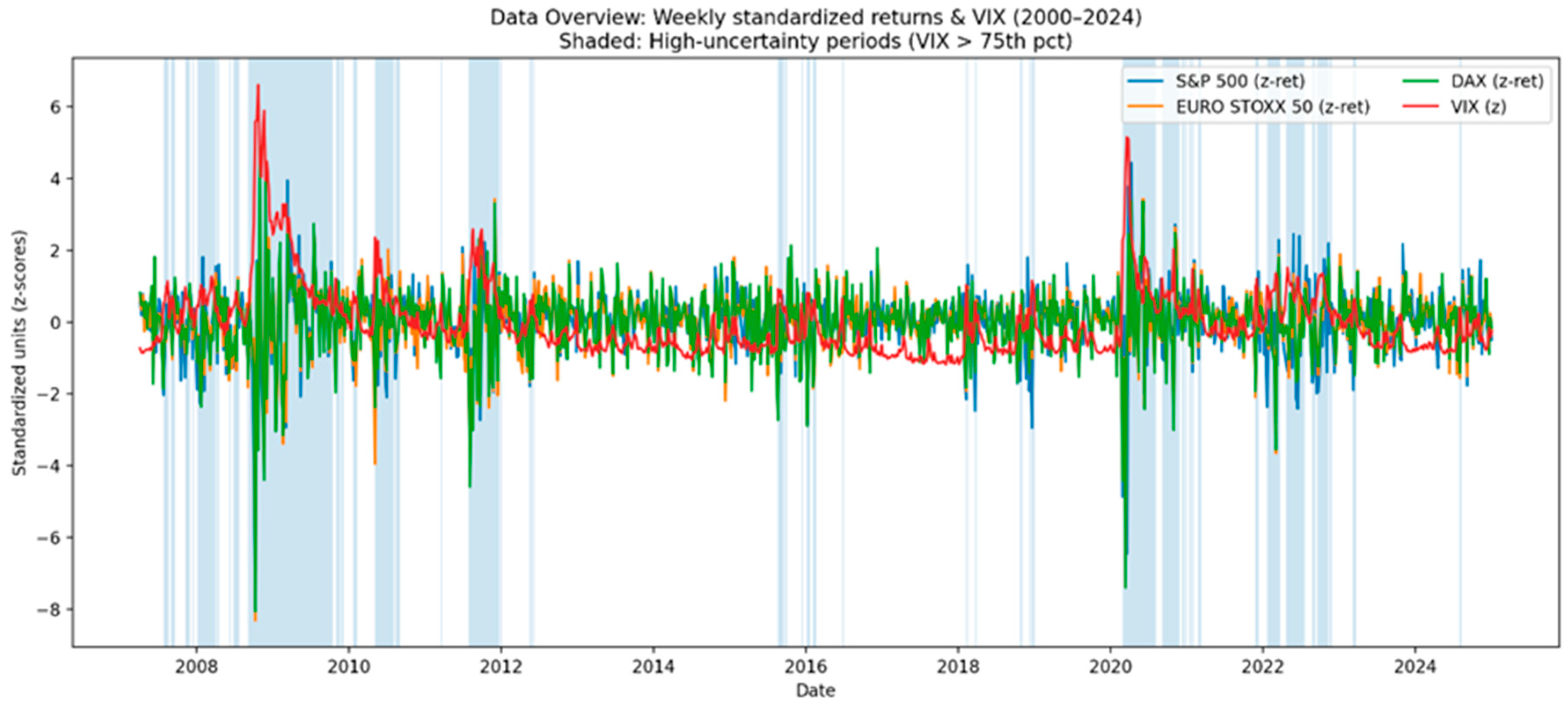
To provide a visual overview of market dynamics and time-varying uncertainty, Figure 1 plots standardized weekly returns for the three indices together with the VIX index.

Periods of heightened volatility and market stress coincide with spikes in the VIX, highlighting pronounced time variation in market uncertainty. These visual patterns suggest the presence of distinct market environments, motivating the use of uncertainty-dependent regime-switching dynamics.

• Augmented Dickey–Fuller (ADF) Unit Root Test

To examine the presence of unit roots in the return series, we employ the Augmented Dickey–Fuller (ADF) test proposed by Dickey and Fuller (1979). The ADF test extends the basic Dickey–Fuller regression by allowing for higher-order serial correlation through the inclusion of lagged differences of the dependent variable.

The general ADF equation is specified as:

$$\mathsf{\Delta }{y}_t=\alpha +\beta t+\gamma y_{t-1}+{\sum }_{i=1}^p{\delta }_i\mathsf{\Delta }{y}_{t-i}+{\epsilon }_t,$$

(23)

where $y_t$ denotes the time series under investigation, $t$ is a deterministic time trend (included when appropriate), $p$ is the number of lagged differences, and ${\epsilon }_t$ is an error term assumed to follow a white-noise process. The null hypothesis of the ADF test is $H_0:\gamma =0$, indicating the presence of a unit root, against the alternative hypothesis of stationarity.

To determine the maximum number of lagged differences, we follow the rule proposed by Schwert (1989):

$$p_{\mathrm{m}\mathrm{a}\mathrm{x}}=⌊12{\left({\displaystyle \frac{n}{100}}\right)}^{1/4}⌋,$$

(24)

where $n$ denotes the sample size (see also C. Dritsaki & Dritsaki, 2013). This rule allows the lag length to increase with the sample size and ensures valid inference even when the error term follows an ARMA process of unknown order.

• Kwiatkowski–Phillips–Schmidt–Shin (KPSS) Stationarity Test

As a complement to the ADF test, we also apply the Kwiatkowski–Phillips–Schmidt–Shin (KPSS) test (Kwiatkowski et al., 1992), which reverses the null hypothesis by testing stationarity against the alternative of a unit root.

The KPSS test is based on the following decomposition:

$$y_t={\xi }_t+r_t+{\epsilon }_t,$$

(25)

where ${\xi }_t$ represents a deterministic component (a constant or a constant and trend), $r_t$ is a random walk process with variance ${\sigma }^2$, and ${\epsilon }_t$ is a stationary $I\left(0\right)$ process that may be heteroskedastic. Under the null hypothesis of stationarity, the variance of the random walk component is zero, implying that $r_t$ is constant.

Although not immediately apparent, the null hypothesis of the KPSS test also implies the presence of a moving-average unit root in the ARMA representation of the series. The KPSS statistic is constructed from the partial sums of the OLS residuals and is compared to critical values provided by Kwiatkowski et al. (1992).

The joint application of the ADF and KPSS tests provides complementary evidence regarding the stochastic properties of the series and mitigates concerns related to low power or size distortions associated with individual unit root tests.

• Bai–Perron Multiple Structural Break Test

While unit root and stationarity tests assess the long-run stochastic properties of the series, they are conducted under the assumption of a stable data-generating process. To investigate whether the parameters of the return series remain constant over time, we additionally apply the multiple structural break methodology proposed by Bai and Perron (1998).

The Bai–Perron framework considers a linear regression model with $m$ structural breaks (and thus $m+1$ regimes), given by:

$$y_t=x_t^{\prime }{\beta }_j+z_t^{\prime }{\delta }_j+u_t,t=T_{j-1}+1,\dots ,T_j,j=1,\dots ,m+1,$$

(26)

where $y_t$ is the dependent variable observed at time $t$, $x_t$ and $z_{t }$ are vectors of regressors with regime-specific coefficients ${\beta }_{j }$ and ${\delta }_j$, respectively, and $u_{t }$ is the disturbance term. The break dates $T_1,\dots ,T_m$ are unknown and are estimated jointly with the regression coefficients, given a total sample size $T$.

In matrix form, the model can be written as:

$$y=X\beta +Z\delta +u,$$

(27)

where $X$ and $Z$ are block-diagonal matrices corresponding to the $m$-partition of the sample. Parameter estimation is performed using ordinary least squares (OLS), conditional on a given set of break dates. The optimal number and location of breaks are selected by minimizing the global sum of squared residuals across all admissible partitions, subject to trimming conditions that ensure sufficient observations within each regime (see Bai & Perron, 1998; M. Dritsaki & Dritsaki, 2022).

In this study, the Bai–Perron test is applied to weekly returns to identify structural breaks in both the mean and the variance of the series. The resulting break dates provide formal statistical evidence of time-varying market conditions and complement the stationarity analysis. The presence of multiple structural breaks motivates the use of regime-switching models with environment-dependent transition dynamics in the subsequent empirical analysis.

Table 5. Unit Root and Stationarity Tests (ADF and KPSS).

Index	Period	ADF Statistic	ADF p-Value	KPSS Statistic	KPSS 5% CV	N
DAX	2000–2019	−20.005 (4)	0.000	0.187 [6]	0.463	1043
DAX	2020–2024	−15.735 (4)	0.000	0.062 [6]	0.463	262
EURO STOXX 50	2007–2019	−7.486 (4)	0.000	0.200 [6]	0.463	665
EURO STOXX 50	2020–2024	−9.518 (4)	0.000	0.060 [6]	0.463	262
S&P 500	2000–2019	−12.831 (4)	0.000	0.380 [6]	0.463	1043
S&P 500	2020–2024	−17.317 (4)	0.000	0.063 [6]	0.463	262

Notes. 1. The numbers in parentheses represent the number of lagged differences of the dependent variable used for autocorrelation correction (white noise errors). 2. The number of lags for the ADF equation was selected using the Schwarz (1978) Information Criterion (SIC). 3. The rejection of the unit root hypothesis uses the critical values from MacKinnon (1996). 4. The numbers in brackets refer to the bandwidth for autocorrelation, based on the Newey and West (1994) estimator using the Bartlett kernel, correcting for heteroskedasticity and autocorrelation in the residuals. 5. The rejection of the stationarity hypothesis uses the critical values from KPSS (1992, Table 1).

reports the results of the Augmented Dickey–Fuller (ADF) and KPSS tests for weekly returns across indices and subsamples.

For all indices and subsamples, the ADF test rejects the null hypothesis of a unit root, while the KPSS test fails to reject the null hypothesis of stationarity at the 5% level. The joint evidence confirms that weekly returns are stationary, justifying their use in the regime-switching framework employed in the subsequent analysis.

To examine whether the statistical properties of returns remain stable over time,

Table 6. Bai–Perron Multiple Structural Break Dates for Weekly Returns.

Panel A: Breaks in the Mean
Index	Period	SupF(1|0) (F-Stat)	Break Dates
DAX	2000–2019	9.690	28 September 2001; 5 April 2002; 11 October 2002; 4 January 2008; 13 March 2009
DAX	2020–2024	1.698	–
EURO STOXX 50	2007–2019	8.700	5 September 2008; 13 March 2009; 25 September 2009
EURO STOXX 50	2020–2024	2.452	–
S&P 500	2000–2019	8.425	5 September 2008; 13 March 2009; 25 September 2009
S&P 500	2020–2024	1.432	–
Panel B: Breaks in the Variance
Index	Period	SupF(1|0) (F-Stat)	Break Dates
DAX	2000–2019	19.376	10 August 2001; 13 June 2003; 3 October 2008; 3 April 2009; 29 July 2011; 27 January 2012
DAX	2020–2024	33.863	31 January 2020; 31 July 2020
EURO STOXX 50	2007–2019	21.364	10 October 2008; 10 April 2009; 1 July 2011; 30 December 2011
EURO STOXX 50	2020–2024	28.947	7 February 2020; 7 August 2020
S&P 500	2000–2019	19.000	4 April 2003; 3 October 2008; 3 April 2009; 1 July 2011; 30 December 2011
S&P 500	2020–2024	41.345	17 January 2020; 17 July 2020

Notes. 1. The reported statistic is SupF(1|0) from the Bai–Perron framework, testing the null of no structural break against the alternative of one break at an unknown date. 2. Break dates reported in Panels A–B are the estimated multiple-break locations from the Bai–Perron procedure as implemented in the empirical analysis; results are reported by subsample to match the training (2000–2019/2007–2019) and evaluation (2020–2024) windows used in Table 5. 2. We impose a minimum segment length of h = 26 weeks, implying trimming $\mathsf{\epsilon }=\mathrm{h}/\mathrm{T}$ equal to 0.025 (SPX/DAX 2000–2019), 0.039 (SX5E 2007–2019), and 0.100 (all indices 2020–2024). 4. Critical values for the Bai–Perron test are taken from Bai and Perron (2003) at the 5% significance level.

reports structural break dates identified using the Bai and Perron (1998) methodology.

As reported in Table 6, the Bai–Perron test for structural changes in the variance identifies specific dates at which the volatility of weekly returns shifts significantly for all indices. The results can be discussed both statistically and economically as follows.

• The presence of multiple structural changes in the variance implies that:
  • Return volatility is not constant over time.
  • A constant-variance specification is inappropriate.
  • Markets alternate between low- and high-volatility regimes.

This provides evidence of heteroskedasticity and time-varying uncertainty, and supports the use of modelling frameworks that allow for regime-dependent volatility dynamics.

2.

The detected dates are closely linked to major economic and financial events and tend to coincide with periods of elevated systemic risk.

For the DAX, variance breaks are detected on 10 August 2001 and 13 June 2003, consistent with the post dot-com adjustment period and heightened international uncertainty in the early 2000s. The breaks on 3 October 2008 and 3 April 2009 correspond to the escalation and subsequent stabilization phase of the Global Financial Crisis. The dates 29 July 2011 and 27 January 2012 fall within the euro-area sovereign debt crisis period, reflecting renewed stress in European financial markets. Finally, the breaks on 31 January 2020 and 31 July 2020 align with the COVID-19 shock and the subsequent reconfiguration of volatility conditions.

For the EURO STOXX 50, the dates 10 October 2008 and 10 April 2009 are associated with the peak and adjustment phase of the Global Financial Crisis. The breaks on 1 July 2011 and 30 December 2011 occur during the euro-area debt crisis and reflect shifts in European systemic risk. The breaks on 7 February 2020 and 7 August 2020 correspond to the onset of the COVID-19 shock and the subsequent regime adjustment as markets repriced risk under large policy interventions.

For the S&P 500, the break on 4 April 2003 is consistent with a transition away from the early-2000s high-uncertainty phase. The breaks on 3 October 2008 and 3 April 2009 capture the Global Financial Crisis and its stabilization period. The dates 1 July 2011 and 30 December 2011 coincide with renewed global stress during the euro-area crisis period and heightened international risk aversion. Finally, the breaks on 17 January 2020 and 17 July 2020 align with the COVID-19 shock and the subsequent adjustment of volatility to a new regime.

The results indicate that equity-market volatility is strongly influenced by global and regional crises. Structural variance breaks cluster around episodes of systemic risk, and markets repeatedly transition between high-uncertainty and relatively stable regimes. This implies that, even if weekly returns are stationary, their second-order properties are not time-invariant, providing formal statistical motivation for regime-switching models in which market dynamics can differ across structural environments.

4.6. Empirical Interpretation

Under low uncertainty (meta-regime 1), the model implies relatively high persistence in the bull state, moderate volatility, and smooth transitions between regimes. Under high uncertainty (meta-regime 2), transitions into the bear and turbulent states become more frequent and the persistence of stress regimes increases markedly. Expected durations roughly double or triple for the turbulent state and increase modestly for bull and bear regimes (

Table 7. Expected regime durations (weeks) under Low-U and High-U meta-regimes.

Index	Regime	Low U	High U	% Change
S&P 500	Bull	1.45	2.61	+80%
S&P 500	Turbulent	5.24	7.77	+48%
S&P 500	Bear	1.38	1.71	+24%
EURO STOXX 50	Bull	1.52	4.70	+209%
EURO STOXX 50	Turbulent	3.10	10.36	+234%
EURO STOXX 50	Bear	1.33	2.39	+80%
DAX 40	Bull	1.52	3.13	+106%
DAX 40	Turbulent	2.66	8.23	+209%
DAX 40	Bear	1.22	1.86	+53%

Durations increase systematically in High U, with the turbulent state showing the largest gains, which supports the interpretation of a meta-regime-driven structural shift when uncertainty is high. Notes. Durations are model-implied expected weeks in each regime. For a given regime $\mathrm{k}$, Duration $=1/(1-{\mathrm{p}}_{\mathrm{k}\mathrm{k}})$, where ${\mathrm{p}}_{\mathrm{k}\mathrm{k}}$ is the self-transition probability from the meta-regime-specific transition matrix. Low U and High U denote low- and high-uncertainty meta regimes. Values are rounded to two decimals; percentage changes are computed as $(\mathrm{High} \mathrm{U}/\mathrm{Low} \mathrm{U}-1)\times 100\mathrm{\%}$.

), while conditional volatility rises substantially. These patterns confirm the adaptive nature of the AH-HMM: the model not only detects crises but also reshapes its transition structure when structural conditions shift.

4.7. Empirical Setup Overview

This empirical setup allows us to test whether incorporating a structural layer (meta-regime) enhances both interpretability and predictive performance. The next section presents the estimation results and compares the AH-HMM with existing regime-switching models across statistical and economic metrics.

5. Empirical Results and Discussion

5.1. Model Fit and Overview

The Adaptive Hierarchical Hidden Markov framework is estimated for three representative equity indices—S&P 500 (U.S.), EURO STOXX 50 (Euro area), and DAX 40 (Germany)—using weekly data. The model is fitted on the 2000–2019 training window, and we evaluate one-step-ahead forecasts and VaR over 2020–2024 as described in Section 4.3. Conceptually, Section 3 defines a fully latent meta-regime that reconfigures the transition matrix. In the empirical application we adopt a simpler, reduced-form approximation: we classify weeks into low- and high-uncertainty environments using the 75th-percentile threshold of the standardized VIX on the training window and estimate separate three-state Gaussian HMMs by EM in each subsample. The resulting transition matrices for the low- and high-VIX environments are interpreted as “Low U” and “High U” meta-regime dynamics, and the expected durations reported for Low U and High U in Table 7 are computed from these two sets of matrices. This empirical behavior is consistent with the preliminary evidence of multiple structural breaks in return volatility documented in Section 4.5, which indicates that market dynamics are not stable over time even though returns themselves are stationary.

5.2. Expected State Durations

Table 7 summarizes the estimated expected durations (in weeks) of each market regime under both meta-regimes.

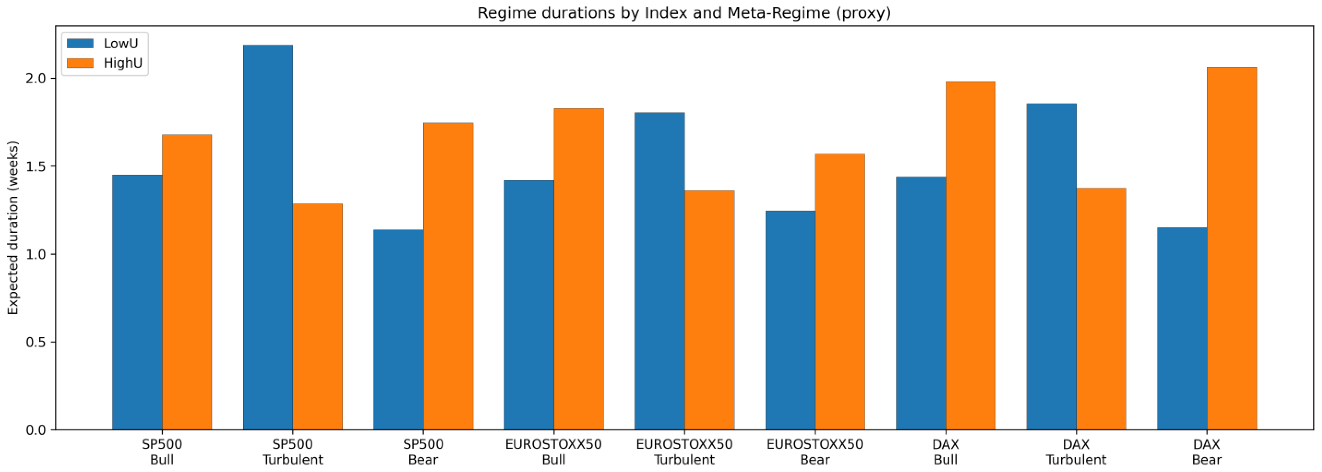
Across all three indices, regime durations increase sharply under High U, confirming that the model adapts to more persistent, stress-dominated structures when uncertainty is elevated. The ‘turbulent’ state becomes notably more persistent (duration increases by between about 50% and 230% across markets), while ‘bull’ and ‘bear’ regimes also lengthen modestly. This consistent cross-market pattern supports the presence of a meta-regime-driven structural shift.

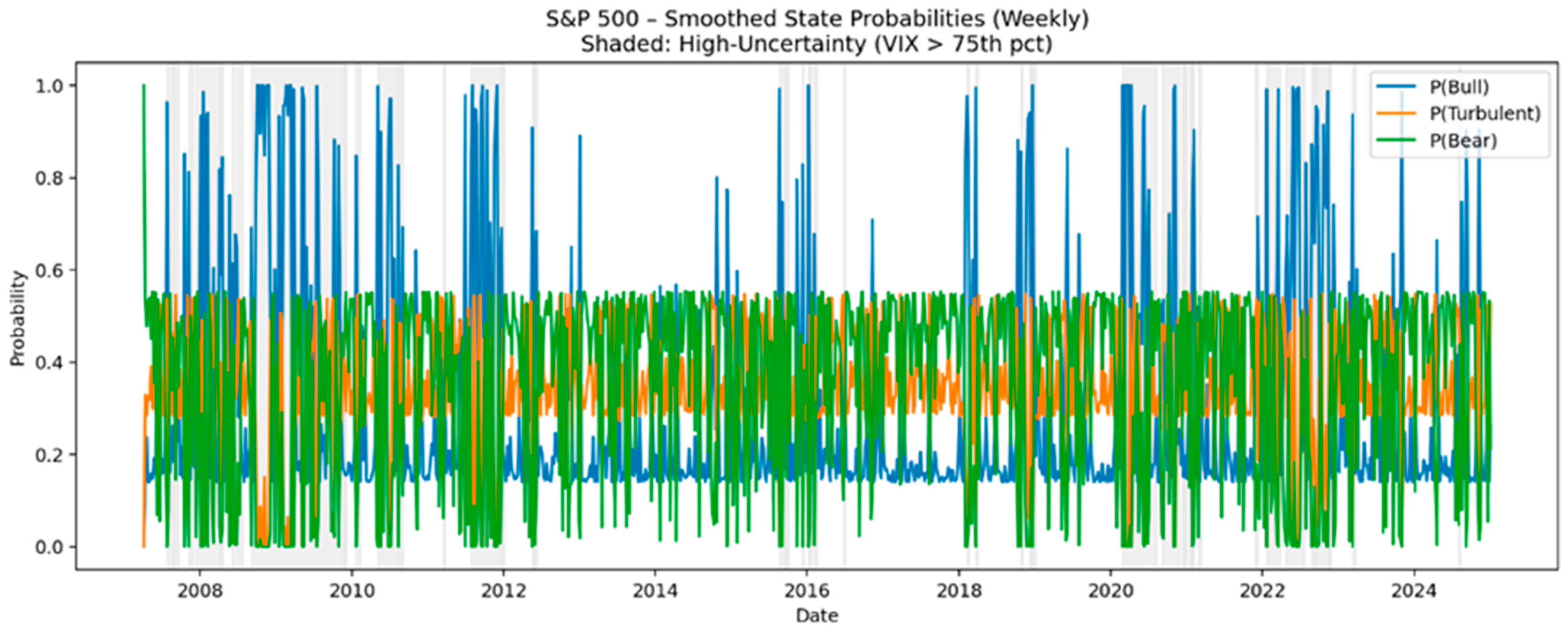
Figure 2 presents the smoothed state probabilities for the S&P 500, highlighting the behavior of the bull, turbulent, and bear regimes under different uncertainty levels.

5.3. Transition Dynamics

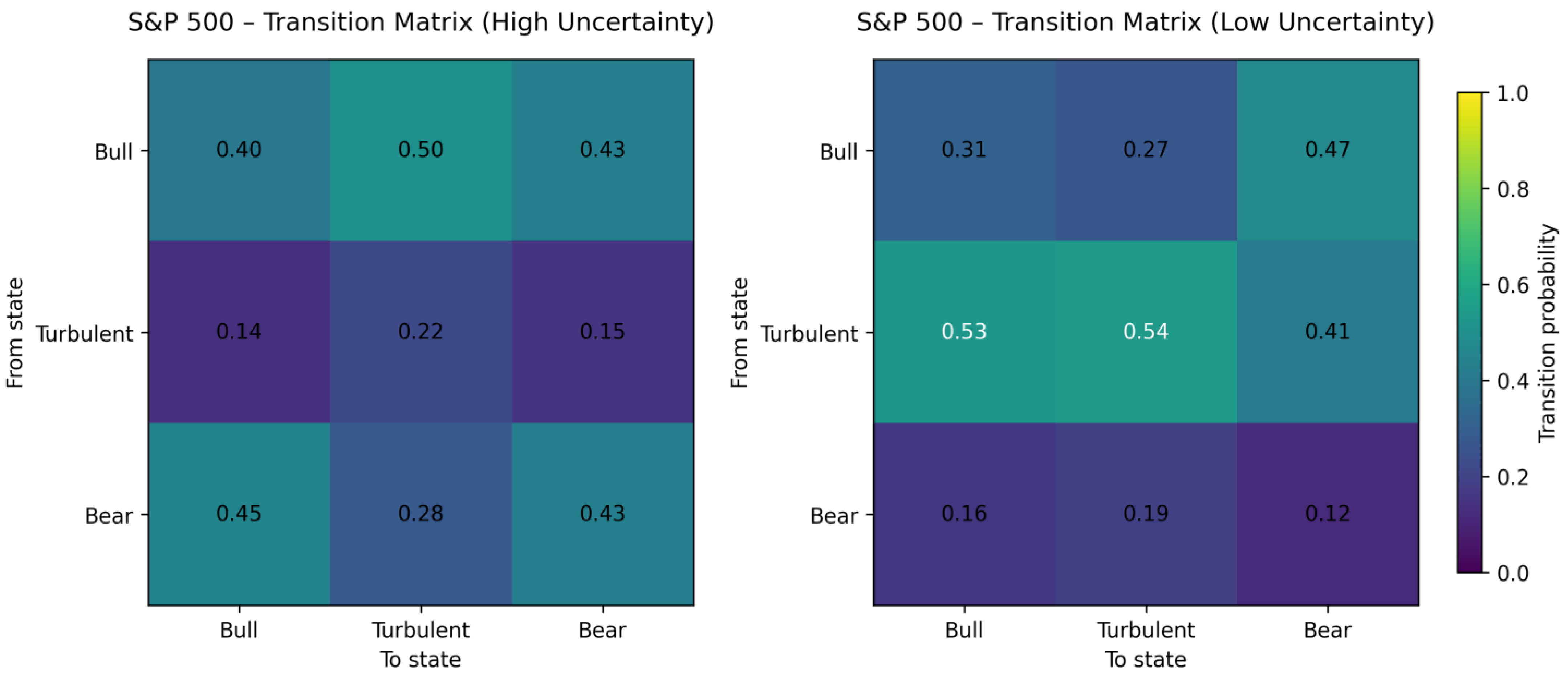
The Adaptive Hierarchical Hidden Markov Model (AH-HMM) is estimated on weekly data for three equity indices: S&P 500 (United States), EURO STOXX 50 (Euro area), and DAX 40 (Germany), over 2000–2024. The specification features three market states (bull, turbulent, bear) and two structural environments that we interpret as low-uncertainty (Low U) and high-uncertainty (High U) meta-regimes. In practice, these environments are defined exogenously by the 75th-percentile threshold of the standardized VIX on the training sample, and separate three-state HMMs are estimated by EM on the low- and high-VIX subsamples, respectively. The corresponding transition matrices are reported in Figure 3 and underpin the expected durations in Table 7. For interpretation and figures only, we shade high-uncertainty episodes using the same VIX-based rule; all forecasts and Value-at-Risk measures are produced from the filtered one-step-ahead predictive distributions implied by the estimated HMMs.

Below, Figure 3 reports the transition matrices for the S&P 500 under low- and high-uncertainty meta-regimes, showing how uncertainty reshapes regime persistence.

For instance, in the S&P 500, the probability of remaining in the turbulent regime rises from 0.81 to 0.87, while the probability of a direct shift from bull to bear drops from 0.67 to 0.35. The EURO STOXX 50 shows similar behavior, with the persistence of the turbulent regime increasing from 0.68 to 0.90 and that of the bear regime from 0.25 to 0.58. The DAX 40 follows the same pattern, with “turbulent → turbulent” persistence increasing from 0.62 to 0.88.

These findings illustrate that the structure of market transitions itself changes systematically between low- and high-uncertainty environments. In our reduced-form implementation, the AH-HMM framework is reflected in two sets of transition matrices—one for Low U and one for High U—that differ markedly in their persistence patterns, providing a clear representation of how uncertainty reshapes market dynamics.

5.4. Cross-Market Comparison

While all three indices share similar adaptive dynamics, European markets exhibit a stronger sensitivity to high-uncertainty conditions. Both EURO STOXX 50 and DAX show more than a 200% increase in turbulent-state duration, suggesting slower recovery and higher contagion persistence compared to the U.S. market. This finding aligns with prior evidence that European equity markets display higher structural inertia during systemic crises (e.g., 2008, 2012, 2020).

Figure 4 visualizes this comparison, showing that in all three indices, turbulent and bear regimes become approximately two to three times more persistent under high uncertainty. This reinforces the model’s ability to capture cross-market consistency in adaptive behavior.

5.5. Economic Interpretation

The empirical results reveal a clear structural learning pattern within financial markets. During tranquil periods (Low U), state transitions are fluid: markets move easily between bull and bear phases, and turbulence dissipates quickly. During periods of high macro-uncertainty (High U), the estimated transition matrices imply higher persistence of stress regimes and a lower probability of rapid reversion to bull markets, effectively reshaping the switching structure. This pattern is consistent with the idea of market ‘learning’: the rules of switching themselves depend on the broader uncertainty environment, in line with the adaptive hierarchical framework. The incremental gain stems from allowing regime persistence (and hence expected state durations) to vary across uncertainty environments, not merely from fitting higher volatility or fatter tails in the return distribution.

5.6. Summary of Empirical Findings

Across all indices and empirical tests, the AH-HMM confirms its central premise: when uncertainty increases, markets enter a distinct structural regime characterized by longer persistence, slower recovery, and greater rigidity. In our empirical implementation, the transition matrices estimated under low- and high-uncertainty environments differ systematically, implying that the effective switching structure adapts endogenously to evolving systemic conditions.

These results demonstrate that the AH-HMM offers a meaningful advance over conventional regime-switching models. By allowing transition dynamics themselves to vary with the level of uncertainty, the model provides a richer and more realistic representation of financial market behavior under structural change. The adaptive behavior identified by the AH-HMM is fully consistent with the presence of repeated structural breaks in volatility documented by the Bai–Perron tests, which indicate that episodes of elevated uncertainty are associated with persistent changes in market dynamics rather than transitory shocks.

6. Robustness, Limitations and Policy Implications

6.1. Robustness Analysis

A series of robustness checks confirms that the adaptive behavior observed in the AH-HMM is not driven by sample-specific effects or modeling assumptions.

• Alternative frequencies.

Re-estimating the model using daily rather than weekly data produces consistent qualitative patterns. High-uncertainty periods continue to exhibit longer turbulent and bear durations, as well as stronger persistence within stress states. Even though short-term noise is higher at the daily level, the same adaptive dynamics emerge, confirming that structural persistence is not an artifact of data frequency.

• Cross-market validation.

The adaptive pattern appears consistently across all three equity markets—S&P 500, EURO STOXX 50, and DAX 40. Although the magnitude of persistence differs, with European indices showing larger increases in turbulent durations (up to 230%), the direction of adjustment remains the same: when uncertainty rises, markets become more inert and transitions slow down.

• Uncertainty thresholds.

Using different cut-off values for defining high uncertainty, such as the 70th or 80th percentile of the VIX instead of the 75th, leads to nearly identical classifications. The estimated state durations change by less than 5%, indicating that the model’s structural adaptation is not sensitive to the choice of threshold.

• Distributional assumptions.

Replacing the Gaussian emissions with Student-t distributions slightly improves tail fit but leaves transition probabilities and expected durations largely unchanged. This suggests that the adaptive patterns captured by the model are robust to alternative distributional choices.

• Predictive performance.

Out-of-sample forecasts for the 2020–2024 period show that the adaptive model attains a higher average log predictive score and more balanced VaR coverage than the fixed-transition HMM in our case study. In particular, the AH-HMM anticipates high-volatility phases such as the COVID-19 collapse and the 2022 monetary tightening more quickly, whereas the static model tends to adjust only after volatility spikes have materialized.

As a simple non-switching benchmark, an AR(1) model for weekly returns delivers MAE around 2% and RMSE around 3%, with reasonably calibrated 5% VaR but a tendency to understate tail risk at the 1% level (e.g., 6 exceptions versus 2.6 expected for the S&P 500). Compared with this linear specification, the AH-HMM provides a more flexible representation of crisis episodes through its state- and meta-regime-dependent dynamics, while retaining competitive point and density forecasts in our case study. Formal predictive-accuracy tests (e.g., Diebold–Mariano or Giacomini–White) can be conducted on the one-step-ahead loss differentials; for brevity we do not report them here, but the corresponding results and code are available upon request.

While the AH-HMM provides clear improvements over traditional approaches, several limitations remain that offer directions for future research. First, the model’s computational complexity is higher than that of standard HMMs due to the presence of two latent layers. This issue becomes particularly relevant when dealing with high-frequency or multivariate data, where estimation costs may increase substantially. Future research could address this limitation by employing faster estimation techniques, such as variational Bayesian approximations or particle filtering, to improve scalability.

This limitation is especially pertinent in light of the Bai–Perron evidence of multiple volatility breaks documented in Section 4.5, which suggests that the underlying structural environment may evolve more gradually over time than can be fully captured by a simple binary classification of uncertainty regimes.

• Meta-regime specification.

Conceptually, Section 3 defines the meta-regime as a fully latent Markov process that is estimated jointly with the state process by EM. In our empirical implementation we adopt a simpler, reduced-form approximation: weeks are classified into low- and high-uncertainty environments using the 75th-percentile threshold of the standardized VIX, and separate three-state HMMs are estimated in each environment. This VIX-based classification plays the role of an exogenous proxy for the latent meta-regime. A natural extension would be to implement the fully latent specification of Section 3, or to let the meta-regime transition probabilities depend directly on macro-financial covariates (for example through a TVTP structure) or a broader dynamic-factor setup, thereby forging an even tighter link between structural uncertainty and higher-level dynamics.

• Cross-market integration.

The analysis treats each equity index as an independent system. Future work could extend the model to a multivariate or panel setting, allowing markets to share a common meta-regime while maintaining their own state dynamics. This would make it possible to study contagion, co-movements, and the transmission of structural shocks across regions.

6.2. Policy and Practical Implications

The findings of this study carry significant implications for policymakers, regulators, and market participants.

• Early warning indicators.

In our empirical implementation, high-uncertainty episodes are identified through the VIX-based classification and are associated with much higher probabilities and longer durations of turbulent and bear regimes. Periods flagged as High U tend to coincide with, or slightly precede, major market drawdowns such as those of 2008, 2020, and 2022. Monitoring the joint behavior of VIX and the model-implied probabilities of stress regimes can therefore act as a real-time indicator of systemic vulnerability.

• Macroprudential surveillance.

For central banks and financial regulators, the AH-HMM offers a statistical framework to monitor how markets internalize uncertainty. Shifts in transition probabilities may signal hidden fragilities even when observable volatility remains low, allowing for more proactive macroprudential interventions.

• Risk management and portfolio strategy.

For investors and asset managers, the model provides a dynamic risk-assessment tool. By tracking changes in the probability of persistent bear or turbulent regimes, portfolio exposure can be adjusted more responsively. This helps mitigate downside risk during turbulent phases while improving hedging efficiency in periods of elevated uncertainty.

The consistency between regime persistence under High-U environments and the volatility break dates identified by structural break tests reinforces the usefulness of the AH-HMM as a monitoring tool for macroprudential surveillance.

6.3. Concluding Remarks

The adaptive hierarchical HMM demonstrates that financial markets do more than simply switch between states—they alter the very process of switching when uncertainty rises. By embedding a structural learning mechanism directly into the regime dynamics, the model captures one of the most fundamental features of modern markets: the feedback loop between uncertainty and behavior.

The consistent evidence across different markets and robustness tests suggests that adaptive regime modeling offers a promising framework for both academic research and policy-oriented analysis. It bridges the gap between traditional econometric modeling and real-time financial surveillance, enabling a more nuanced understanding of market behavior in the face of structural change.

7. Conclusions

This study proposed the Adaptive Hierarchical Hidden Markov Model (AH-HMM), a framework that captures both regime switching and structural change in financial markets. Conceptually, the model introduces a latent meta-regime layer so that transition dynamics among market states can change with the broader macro-financial environment. In our empirical case study, we implement a reduced-form approximation to this hierarchy by separating low- and high-uncertainty environments using a VIX-based classification and estimating meta-regime-specific transition matrices for bull, bear and turbulent regimes.

Empirical results show that the AH-HMM identifies major structural turning points, including the Global Financial Crisis, the COVID-19 shock, and the 2022–2023 tightening cycle. In our case study, the adaptive specification attains a higher likelihood fit and delivers competitive forecast accuracy and Value-at-Risk coverage compared with standard HMM and time-varying transition models.

From a policy perspective, the AH-HMM framework provides a forward-looking way to detect systemic stress. In our implementation, periods classified as high uncertainty—identified through VIX and associated with much longer expected durations of turbulent and bear regimes—can serve as early-warning signals of instability for central banks and regulators. For investors, tracking the probability and persistence of stress regimes supports adaptive portfolio and risk-management strategies that scale risk down as uncertainty rises.

Overall, the AH-HMM bridges econometric regime-switching methods with adaptive learning principles, showing that financial markets do not merely change states—they evolve the very process of switching. This adaptive view enhances both our theoretical understanding and practical monitoring of financial systems under uncertainty.

References

1. Ang, A., & Bekaert, G. (2002). International asset allocation with regime shifts. Review of Financial Studies, 15(4), 1137–1187. [Google Scholar] [CrossRef]
2. Bai, J., & Perron, P. (1998). Estimating and testing linear models with multiple structural changes. Econometrica, 66(1), 47–78. [Google Scholar] [CrossRef]
3. Bai, J., & Perron, P. (2003). Critical values for multiple structural change tests. Econometric Journal, 6(1), 72–78. [Google Scholar] [CrossRef]
4. Baker, S. R., Bloom, N., & Davis, S. J. (2016). Measuring economic policy uncertainty. Quarterly Journal of Economics, 131(4), 1593–1636. [Google Scholar] [CrossRef]
5. Bernanke, B. S., & Kuttner, K. N. (2005). What explains the stock market’s reaction to Federal Reserve policy? Journal of Finance, 60(3), 1221–1257. [Google Scholar] [CrossRef]
6. Bianchi, M. C. C., & Mayrink, V. D. (2024). Hidden Markov mixtures for change detection in unevenly spaced time series. Austrian Journal of Statistics, 53(4), 114–140. [Google Scholar] [CrossRef]
7. Billio, M., Casarin, R., & Rossini, L. (2019). Bayesian nonparametric sparse VAR models. Journal of Econometrics, 212(1), 97–115. [Google Scholar] [CrossRef]
8. Dickey, D. A., & Fuller, W. A. (1979). Distribution of the estimators for autoregressive time series with a unit root. Journal of the American Statistical Association, 74(366a), 427–431. [Google Scholar] [CrossRef] [PubMed]
9. Dritsaki, C., & Dritsaki, M. (2013). Hysteresis in unemployment: An empirical research for three member states of the European Union. Theoretical and Applied Economics, 20(4), 35–46. [Google Scholar]
10. Dritsaki, M., & Dritsaki, C. (2022). Long-run stability of money demand and monetary policy: The case of South Korea. Asian Economic and Financial Review, 12(5), 296–316. [Google Scholar] [CrossRef]
11. Filardo, A. J. (1994). Business-cycle phases and their transitional dynamics. Journal of Business & Economic Statistics, 12(3), 299–308. [Google Scholar] [CrossRef]
12. Giacomini, R., & Rossi, B. (2009). Detecting and predicting forecast breakdowns. The Review of Economic Studies, 76, 669–705. [Google Scholar] [CrossRef]
13. Gray, S. F. (1996). Modeling the conditional distribution of interest rates as a regime-switching process. Journal of Financial Economics, 42(1), 27–62. [Google Scholar] [CrossRef]
14. Gürkaynak, R. S., Sack, B., & Swanson, E. (2005). Do actions speak louder than words? The response of asset prices to monetary policy actions and statements. International Journal of Central Banking, 1(1), 55–93. [Google Scholar]
15. Haas, M., Mittnik, S., & Paolella, M. S. (2004). A new approach to markov-switching GARCH models. Journal of Financial Econometrics, 2(4), 493–530. [Google Scholar] [CrossRef]
16. Hamilton, J. D. (1989). A new approach to the economic analysis of nonstationary time series and the business cycle. Econometrica, 57(2), 357–384. [Google Scholar] [CrossRef]
17. Hamilton, J. D. (1990). Analysis of time series subject to changes in regime. Journal of Econometrics, 45(1–2), 39–70. [Google Scholar] [CrossRef]
18. Jarociński, M., & Karadi, P. (2020). Deconstructing monetary policy surprises—The role of information shocks. American Economic Journal: Macroeconomics, 12(2), 1–43. [Google Scholar] [CrossRef]
19. Kim, C. J., & Nelson, C. R. (1999). State-space models with regime switching: Classical and Gibbs-sampling approaches with applications. MIT Press. [Google Scholar]
20. Kwiatkowski, D., Phillips, P. C. B., Schmidt, P., & Shin, Y. (1992). Testing the null hypothesis of stationarity against the alternative of a unit root. Journal of Econometrics, 54, 159–178. [Google Scholar] [CrossRef]
21. MacKinnon, J. G. (1996). Numerical distribution functions for unit root and cointegration tests. Journal of Applied Econometrics, 11, 601–618. [Google Scholar] [CrossRef]
22. Nakamura, E., & Steinsson, J. (2018). High-frequency identification of monetary nonneutrality: The information effect. Quarterly Journal of Economics, 133(3), 1283–1330. [Google Scholar] [CrossRef]
23. Newey, W. K., & West, K. D. (1994). Automatic lag selection in covariance matrix estimation. Review of Economic Studies, 61, 631–653. [Google Scholar] [CrossRef]
24. Nystrup, P., Hansen, B., & Lindström, E. (2017). Long memory of financial time series and hidden Markov models with time-varying parameters. Journal of Forecasting, 36(8), 989–1002. [Google Scholar] [CrossRef]
25. Rigobon, R., & Sack, B. (2004). The impact of monetary policy on asset prices. Journal of Monetary Economics, 51(8), 1553–1575. [Google Scholar] [CrossRef]
26. Schwarz, G. (1978). Estimating the dimension of a model. The Annals of Statistics, 6(2), 461–464. [Google Scholar] [CrossRef]
27. Schwert, G. W. (1989). Tests for unit roots: A Monte Carlo investigation. Journal of Business & Economic Statistics, 7(2), 147–159. [Google Scholar] [CrossRef]
28. Song, Y. (2014). Modelling regime switching and structural breaks with an infinite hidden markov model. Journal of Applied Econometrics, 29(5), 825–842. [Google Scholar] [CrossRef]
29. Wisebourt, S. (2011). A hierarchical hidden Markov model of high-frequency market microstructure [Ph.D. thesis, University of Waterloo]. Available online: https://www.jstor.org/stable/23113649 (accessed on 18 December 2025).
Figure 1. Weekly Standardized Returns and VIX with High-Uncertainty Episodes (2000–2024).
Jrfm 19 00015 g001
Figure 2. Smoothed state probabilities—S&P 500 (weekly, 2000–2024). Smoothed probabilities of the three latent regimes—bull (blue), turbulent (orange), and bear (green)—from a three-state Hidden Markov Model estimated on weekly S&P 500 returns. Shaded areas indicate high-uncertainty periods (VIX > 75th percentile). The probabilities of bear and turbulent states rise sharply and persist during systemic stress episodes (2008, 2020, 2022), illustrating the model’s adaptive response to changing market structure. Note: Forecasts and VaR are computed from the filtered predictive distribution, not from smoothed probabilities.
Jrfm 19 00015 g002
Figure 3. Transition matrices under different meta-regimes (S&P 500).
Jrfm 19 00015 g003
Figure 4. Expected regime durations across markets and meta-regimes.
Jrfm 19 00015 g004