Article

Bank Leverage Restrictions in General Equilibrium: Solving for Sectoral Value Functions

by
Brittany Almquist Lewis
Olin Business School, Washington University, St. Louis, MO 63130, USA
J. Risk Financial Manag. 2025, 18(9), 519; https://doi.org/10.3390/jrfm18090519
Submission received: 10 July 2025 / Revised: 31 August 2025 / Accepted: 1 September 2025 / Published: 17 September 2025
(This article belongs to the Special Issue Financial Resilience in Turbulent Times)

Abstract

This paper develops a tractable method to solve a general equilibrium model with bank runs and exogenous leverage ratio restrictions, enabling welfare analysis of macroprudential policy across the business cycle. By computing bankers’ value functions via backward induction from steady state, the framework quantifies how leverage caps affect capital allocation, asset prices, and run probabilities during recovery from crises. Calibrated simulations show that welfare-enhancing policy is time-varying—lenient when households’ marginal utility of consumption is high, and restrictive in low-marginal-utility states. The results highlight a trade-off: tighter leverage restrictions improve stability but risk persistent efficiency losses if imposed too harshly after crises.

1. Introduction

The Global Financial Crisis triggered rigorous debate on the bank regulation necessary to increase stability in the financial sector. The Basel Committee on Banking Supervision agreed on reforms, including a non-risk-based leverage ratio requirement for financial institutions, to be introduced in 2013 in Basel III.1 Basel III scheduled a phase-in of this leverage requirement at an initial 3% equity-to-assets, with finalization in 2018. In 2014, as part of the implementation of Basel III, U.S. banking regulators introduced the Supplementary Leverage Ratio (SLR), a non-risk-based leverage ratio restriction projected to reach up to 6% equity-to-assets—including off-balance sheet exposures2—for globally systemically important depository banks.3 However, the optimal level for these leverage restrictions is not well understood4—evidenced by the SLR’s temporary relaxation to facilitate financial intermediation during the COVID pandemic, and the 2025 proposal to recalibrate it.
This paper examines whether leverage ratio restrictions can balance the trade-off between increased banking-sector stability and allocational efficiency losses in a welfare-improving way. I interpret systemic risk as an economy-wide run on the banking sector, following Gertler and Kiyotaki (2015). I add exogenous leverage restrictions to an infinite-horizon general equilibrium model with bank runs and an endogenous price of capital, and examine the effects of such restrictions.
Following a crisis, banks must increase leverage to restore their efficient capital holdings, but higher leverage raises the probability of a run. Crises occur endogenously as economy-wide bank runs. In the immediate aftermath of a crisis, high returns on bank assets loosen collateral constraints, enabling very high leverage—precisely when the economy is most fragile. In the model’s multiple-equilibria framework, run probability rises with leverage if post-run bank assets cannot cover liabilities. Banks fail to internalize how their leverage choices affect run risk, creating scope for welfare-improving leverage restrictions.
In this multiple equilibria model, the bank run equilibrium arises partly from liquidity mismatch—short-term liabilities funding partially illiquid long-term assets—akin to Diamond and Dybvig (1983). This model studies a crisis like the Global Financial Crisis, which was a rollover crisis in the same vein as the sovereign debt crisis studied by Cole and Kehoe (2000). If all depositors roll over funds, banks can buy capital from inefficient holders, raising the price of capital and loosening the banks’ participation constraint, which sustains lending. However, if a sunspot causes widespread non-rollover, banks purchase too little capital to generate the expected price increase, banker incentives collapse, and depositors seize their deposits. In each period, there is some probability of such a coordination failure.
The banks in this model correspond to lightly regulated ”shadow” banks or net-borrowing banks in the unsecured interbank market. These banks were largely funded by short-term unsecured loans, which will correspond to deposits in this model. I solve for the post-run recovery path with and without leverage caps, comparing stability and real-economy outcomes across these regimes. The most effective leverage restriction is time-varying: it should be least restrictive when households’ marginal utility of consumption is highest, and more restrictive as their marginal utility approaches steady-state levels. Overly tight post-run leverage restrictions reduce welfare by slowing banks’ repurchase of capital, depressing production, asset prices, and net worth. In contrast, a time-varying cap—more lenient during high marginal utility periods—improves welfare relative to laissez-faire value of leverage.
A technical contribution of this paper is a solution method that dynamically computes household and bank value functions via backward induction from the steady state. I then use a recursion that iterates one period backward at a time to solve for the bankers’ value function at each previous period in the bank-run-to-steady-state transition path. This recursive specification enables solving the model with an exogenous leverage restriction and testing alternative macroprudential leverage regimes along the transition from a bank run to the bank’s steady state. This direct calculation of the banks’ value function informs the maximum leverage that households are willing to lend, and by comparing it to an exogenous restriction, the model endogenously determines whether regulation binds in each period.
This approach enables quantitative evaluation of macroprudential policy. I calibrate the model to approximate pre-GFC economic parameters and simulate the model to understand the dynamics at play under varying leverage caps. This exercise is instructive for understanding how economic variables respond to varying leverage restriction regimes, including one inspired by the SLR, and the implications for the size and stability of the banking system under each regime. The model facilitates testing whether leverage ratio restrictions balance the trade-off between increased stability in the banking sector and allocational efficiency losses in a welfare-improving way.
Extensions to this framework could be utilized to explore how changes in the bankruptcy code’s treatment of collateral in the sale and repurchase (“repo”) market offset macroprudential policy by affecting dealer-bank repo leverage. In 2005, Congress extended the exemption from the automatic stay—granting “super-senior” bankruptcy status—to repos backed by mortgage collateral. Lewis (2023) documents the mechanism through which this change amplified the boom–bust cycle leading up to the Global Financial Crisis (GFC) and shows that the reform generated a repo money multiplier that expanded bank leverage and credit supply to the housing market. Lewis (2021) documents that the resulting mortgage originations exhibited riskier contract structures, were disproportionately concentrated in minority-dominant zip codes, and experienced elevated default and foreclosure rates––increasing the risk of runs on the mortgage-backed repos that they underpinned. Consistently, Gorton and Metrick (2012) argue that repo runs were at the nexus of the GFC, and Roe (2010) referred to the 2005 bankruptcy code change as a “financial crisis accelerator”.
Since the general equilibrium model developed in this paper internalizes bank runs as the source of risk created by leverage, it is well-suited for studying leverage in the repo market. By incorporating dealer-bank leverage, the cost of capital, and bank-run dynamics, the model provides a natural framework for evaluating the potential credit market effects and financial instability created by changes to repo treatment in bankruptcy law.
If future changes to the bankruptcy code expand the definition of repurchase agreements—and thus expand exemption from automatic stay—to include assets such as commercial real estate (CRE) loans or collateralized loan obligations (CLOs), a similar credit cycle—characterized by rapid expansion followed by contraction—could arise, akin to that observed during the GFC. In commercial real estate, for example, the evidence in Lewis (2021, 2023) suggests that the dynamics would involve an expansion of lending, increased risk of the newly originated loans, an influx of capital into that sector via the tri-party repo market, and increased vulnerability to repo runs.5 Thus, extensions of this model provide a framework to evaluate the effects of proposed changes to the bankruptcy treatment of repo collateral.
This paper contributes to two strands of literature. It contributes to an important literature on banking panics (see e.g., Acharya et al., 2011; Arfaoui & Uhlig, 2025; Diamond & Dybvig, 1983; Ennis & Keister, 2010; Gorton & Ordonez, 2020; He & Krishnamurthy, 2012). Much of this literature builds on the conventional financial accelerator model of Bernanke et al. (1999) and Kiyotaki and Moore (1997). This paper internalizes bank runs—modeled as a role over panic similar to Cole and Kehoe (2000)—as the source of risk inherent in bank leverage, in the same vein as in Gertler and Kiyotaki (2015). Relative to Gertler and Kiyotaki (2015), I incorporate banks and households into a single family, which allows me to evaluate economic welfare under alternative leverage restrictions. In later work, Gertler et al. (2020) solve for the optimal leverage restriction numerically. The model in my paper differs from that in Gertler et al. (2020) by removing equity injections and credit booms in the form of productivity shocks, which helps to simplify the model to focus on the economic impact of leverage restrictions on real variables. My paper offers a contribution to the model by calculating the bankers’ value function in steady state as a geometric series of steady state variables. I then solve for the value function at each previous period in the bank-run-to-steady-state transition path by setting up a recursion that iterates one period backward at a time. This recursive specification facilitates solving the model with an exogenous leverage restriction and testing alternative macroprudential leverage regimes along the transition path. I test three leverage restriction regimes: binding only one period after a bank run, binding for multiple post-run periods, and binding only in steady state periods. I also introduce new stability metrics from a 10,000-period simulation: time between runs, time in steady state, and time to reach steady state. Christiano et al. (2022) find that this model is highly non-linear and difficult to solve; thus, the contribution I provide offers a meaningful improvement in the ability to solve this model.
This paper is related to work that quantifies the effects of capital requirements and leverage constraints (see, e.g., Christiano & Ikeda, 2016; De Nicolò et al., 2014; Martinez-Miera & Suarez, 2014; Nguyen, 2015). Using a quantitative general equilibrium growth model to quantify the welfare costs of capital requirements, Van den Heuvel (2008) finds that the welfare costs of capital requirements are large, while Begenau (2020) finds that US capital requirements have been suboptimally low. This paper innovates by studying welfare under varying capital requirement regimes in a general equilibrium model with credit cycles. I find evidence consistent with the optimal leverage restriction being time-varying across the business cycle. When the household’s marginal utility of consumption is highest, the leverage ratio requirement should be the least restrictive. Conversely, when the household’s marginal utility approaches its steady state level, the optimal leverage ratio becomes more restrictive. I also offer additional metrics about the equilibrium variables under varying leverage restrictions.

2. Model

This is an infinite-horizon model of the macroeconomy with a banking sector where I enhance the model of Gertler and Kiyotaki (2015) to account for bank regulation in the form of leverage ratio restrictions, similar to Gertler et al. (2020).
Each period, there are two possible states of the world: a bank-run state and a non-bank-run state, and the bank runs are anticipated. There are two types of agents, households and bankers; each type of agent has a continuum of measure unity. The productive technology in the economy is f ( K t ) = Z K t . In the bank-run state, all of the households run on the entire banking sector. I will focus on the case where, if a bank run materializes, the banks do not have sufficient assets to cover their liabilities. This means that the households will receive a fraction of their original deposits, and the price of capital during the bank run, Q * , drops as banks sell their capital at fire sale prices to the inefficient households. These price changes for both deposits and capital affect the household’s budget constraint.
This is a two-good economy: there is capital, the durable good, and there is the consumption good, which is a non-durable good. The paper abstracts from capital accumulation, so there is a fixed supply of capital each period, and it does not depreciate:
K t b + K t h = 1
Both bankers and households have production functions ( f B and f H , respectively). Households require both capital and units of the consumption good as inputs in order to produce more units of the consumption good. In other words, the households pay a cost in consumption goods for operating capital. I will suppose that this cost is a convex, increasing function of their capital holdings:
f H ( K t h , f ( K t h ) ) = Z K t h
where I assume:
f ( K t h ) = α 2 ( K t h ) 2
K t h units of capital remain.
The bankers are efficient users of capital; they only require capital-good inputs in order to produce more units of the consumption good.
f B ( K t b ) = Z K t b
K t b units of capital remain.
When households sell more capital to the banks, the amount of consumption goods in the economy increases, since the banks are more efficient at producing capital. Therefore, in the absence of financial frictions, banks would intermediate all of the capital stock. However, when the banks are constrained in their ability to borrow funds to purchase the capital, the households will directly hold some of the capital. When the financial constraints tighten on the bank, the households will be forced to hold an elevated supply of capital.
However, lending to the bank is risky because there is a probability of an economy-wide bank run each period. The probability of a bank run depends on the amount of leverage that the banks have. The probability of a bank run, p t , impacts the price of both capital and deposits. It also affects the banker’s value function, which is calculated as the banker’s return from operating honestly each period in the future, given that there is no bank run. When a bank run occurs, banks are liquidated, and due to borrowing constraints, once they have zero net worth, they will never be able to take deposits again.

2.1. Households

The households both consume and save. The households can save either by lending funds to the competitive financial institutions, the banks, or by holding the capital directly. Every period, households receive a return on their asset holdings as well as an endowment of the consumption good, Z W h . This setup allows the household endowment to vary proportionally with the aggregate productivity, Z.
Deposits held by the banks are one-period bonds. In the non-bank-run state, these bonds yield a non-contingent rate of return R t . However, in the bank-run state, these assets receive only a fraction x t + 1 of the promised return, where x t + 1 is the total liquidation value of bank assets per unit of promised deposit. Thus, the household’s return on deposits can be expressed as:
R t = R ¯ t if no bank run , x t + 1 R ¯ t if bank run occurs
where 0 x t < 1 . In the run state, all depositors receive the same pro rata share of liquidated assets. Unlike in Diamond and Dybvig (1983), there is no sequential service constraint on the depositor contract that links payoffs in the run state to depositors’ place in line.
Household utility, U t , is given by:
U t = E t i = 0 β i ln C t + i h
where C t h is household consumption, 0 < β < 1 , and Q t is the market price of capital. The household chooses consumption, bank deposits, D t , and direct capital holdings, K t h , to maximize expected utility subject to the budget constraint:
C t h + D t + Q t K t h + f ( K t h ) = Z t W h + R t D t 1 + ( Z t + Q t ) K t 1 h + ( 1 σ ) N t
Suppose that p t is the probability that households assign to an economy-wide bank run occurring at time t + 1 (a discussion of how p t is determined will follow). Since the households anticipate that a bank run will occur with positive probability, the rate of return promised on deposits, R t + 1 , must satisfy the household’s first order condition for deposits:
1 = R t + 1 E t ( 1 p t ) Λ t , t + 1 + p t Λ t , t + 1 * x t + 1
where Λ t , t + 1 * = β C t h C t + 1 h * is the household’s intertemporal marginal rate of substitution conditional on a bank run at t + 1 . The depositor recovery rate, x t + 1 , in the event of a run depends on the rate of return promised on deposits, R t + 1 .
x t + 1 = min 1 , ( Q t + 1 * + Z t + 1 ) k t b R t + 1 d t
Following Gertler and Kiyotaki (2015), in the spirit of the global games approach developed by Morris and Shin (1998) and applied to banks by Goldstein and Pauzner (2005), I postulate a reduced form that relates the probability of a bank run, p t , to the aggregate recovery rate, x t + 1 . In this way, the probability p t of the “sunspot” bank run outcome depends in a natural way on the fundamental x t + 1 . In general, the probability that depositors assign to a bank run occurring in the following period is a decreasing function of the recovery rate:
p t = g ( E t ( x t + 1 ) ) with g ( · ) < 0 0 if E t ( x t + 1 ) = 1
where g follows the simple linear form:
g ( · ) = 1 E t ( x t + 1 )
Higher leverage chosen by banks today will decrease the recovery rate tomorrow, which increases the probability of a bank run occurring tomorrow. This increases R t + 1 , the rate of return households require to hold assets from today until tomorrow. Therefore, when the bank is choosing leverage to maximize its value function, the cost of deposits owed at t + 1 , R t + 1 , will affect the bank’s decision on how much leverage to take on. Thus, banks internalize the impact that their choice of leverage has on p t only indirectly through its effect on R t + 1 .

2.2. Banks

Banks in this paper correspond to lightly regulated “shadow” banks or net-borrowing banks in the unsecured interbank market, similar to the setting described in Lewis (2021, 2023). These banks hold long-term securities and issue short-term debt, which makes them vulnerable to bank runs. Each banker manages a financial intermediary. Bankers fund their capital investments by issuing deposits to households, as well as by investing their own net worth, n t .
Bankers may be constrained in their ability to borrow deposits, and will attempt to save their way out of the financial constraints by accumulating their retained earnings. To limit the possibility that bankers will try to move towards one hundred percent equity financing, bankers have a finite expected lifetime. Each banker has an i.i.d. probability σ of surviving until the next period, and a probability 1 σ of exiting at the end of the current period. The expected lifetime of a banker is then 1 1 σ .
Each period, new bankers enter with an endowment w b which is received only in their first period of life. The number of entering bankers is equal to the number who exit, keeping the total number of bankers constant. Bankers are risk-neutral, and they will rebate their entire net worth to the households, as I discuss in detail later in the paper, in the period that they exit. Thus, the expected utility of a continuing banker at the end of period t is given by:
V t = E t i = 1 β i ( 1 σ ) σ i 1 Π t + i n t + i
where ( 1 σ ) σ i 1 is the probability of a banker exiting at date t + i , n t + i is the banker’s terminal net worth upon exiting in period t + i , and Π t + i is the household’s marginal utility of consumption in period t + i . The bankers take the household’s marginal utility of consumption as given.
Conditional on the productivity Z, the net worth of the “surviving” bankers is the gross return on assets net the cost of deposits. Banks can only increase their net worth using their retained earnings. This friction is a reasonable approximation of banks in reality. In this paper, however, I keep Z constant across time. An area for future analysis would be to explore the effects of shocking productivity Z.
n t + 1 = Z + Q t + 1 k t b R t + 1 d t
Exiting bankers no longer operate their banks, and they rebate their net worth to the households in the period that they exit. Each period t, new and surviving bankers finance their asset holdings Q t k t b with newly issued deposits and net worth:
Q t k t b = n t + d t
There is a limit to the amount of deposits that bankers can borrow in a given period. This constraint can be motivated by assuming that a moral hazard problem exists. In time t, after accepting the deposits, but still during the same period, the banker chooses whether to operate “honestly” or to divert the assets for his personal use. Operating honestly requires the banker to invest the deposits, wait until the next period, realize the returns on deposits, and meet all deposit obligations. If the banker chooses to divert the assets, he will only be able to liquidate up to the fraction θ of the assets, and he will only be able to do so slowly, in order to remain undetected. Therefore, the banker must decide whether to divert at time t. The cost of diverting assets is that the depositors are able to force the banker into bankruptcy in the next period. Therefore, at time t, the bankers decide whether or not to divert the assets by comparing the franchise value of the financial intermediaries that they operate, V t , to the potential gains from diverting funds θ t Q t k t b , where V t is calculated as the present discounted value of the future payouts from operating the bank honestly every period. Any rational depositor will not lend deposits to a banker who has an incentive to divert funds. Therefore, the following incentive constraint on the banker must hold.
θ t Q t k t b V t
Given that bankers consume their net worth in the period that they exit, their franchise value can be restated recursively as the expected discounted value of the sum of their net worth conditional on exiting in the following period, plus their franchise value conditional on continuing in the following period.
V t = E t β ( 1 σ ) Π t + 1 n t + 1 + β σ V t + 1
Thus, the banker’s optimization problem is to choose ( k t b , d t ) each period to maximize the franchise value subject to the incentive constraint and the balance sheet constraints. As long as the return on bank capital is greater than the banks’ cost of deposits, banks will have an incentive to take on the maximum amount of leverage available to them.
ϕ t = ψ t θ
Since both the banker objective function and constraints are constant returns to scale, the optimization problem can be reduced to choosing the leverage multiple, ϕ t , to maximize the bank’s “Tobin’s q ratio”, V t n t ψ t .

2.3. Aggregation

Given that the leverage multiple ϕ t is independent of individual bank-specific factors, and given a parameterization where the banker incentive constraint is binding in equilibrium, then the banks can be aggregated to yield the following relationship between total assets held by the banking system and total net worth:
θ t Q t K t b = V t .
The evolution of N t is given by the sum of surviving and entering bankers as:
N t + 1 = σ ( Z + Q t + 1 ) K t b R t + 1 D t + W b .
where W b = ( 1 σ ) w b is the total endowment across all entering bankers, and the first term is the accumulated net worth of bankers that were operating at period t and survived until period t + 1 . Conversely, exiting bankers rebate the fraction ( 1 σ ) of accumulated net worth back to the households.
Total output Y t is equal to the sum of output from capital Z , household endowment Z W h , and W b .
Y t = Z + Z W h + W b
The output is either used to pay capital management costs or for household consumption:
Y t = f ( K t h ) + C t h .
The household marginal utility of consumption can be defined as follows:
Π t = 1 C t h

2.4. Adding an Exogenous Leverage Constraint to the Model

To evaluate leverage ratio restrictions using this model, I add an exogenous leverage restriction that is more restrictive than the endogenous leverage restriction, which arises due to the agency problem that bankers face. I then analyze varying leverage ratio restrictions numerically in Section 3.
Introducing the exogenous leverage restriction to the model adds an additional constraint to the banker’s optimization problem. Now, bankers must maximize their normalized value function subject to both their endogenous participation constraint as well as the exogenous leverage restriction ( ϕ ¯ t ) .
ψ t = max ϕ t E t β ( 1 σ ) Π t + 1 + β σ ψ t + 1 N t + 1 N t s . t .
θ ϕ t ψ t ϕ t ϕ ¯ t , for each t
Taking expectations over the probability that there is no bank run each period, and given that the return on bank capital holdings is greater than the cost of deposits,
Z + Q t + 1 Q t R t 0
bankers maximize their value function by choosing the maximum amount of leverage so that, at the optimum, their value function can be written as follows:
ψ t = min 1 , ( Z + Q t + 1 * ) K t b ( min { ψ t θ , ϕ ¯ t } 1 ) N t R t × β ( 1 σ ) Π t + 1 + σ ψ t + 1 × min { ψ t θ , ϕ ¯ t } ( Z + Q t + 1 ) Q t ( min { ψ t θ , ϕ ¯ t } 1 ) R t
This means that optimal choice of leverage is no longer equal to ϕ t = ψ θ ; it is now equal to the minimum of this value and the exogenous leverage restriction. Therefore, in order to determine leverage, I must first model the banker’s value function in order to know which constraint will bind. The bankers’ value function is:
V t = E t i = 1 β i ( 1 σ ) σ i 1 Π t + i N t + i
Given the law of motion of n t ,
n t + 1 = n t ϕ t Z + Q t + 1 Q t ( ϕ t 1 ) R t and n t + i = n t a = 1 i ϕ t + a 1 Z + Q t + a Q t + a 1 ( ϕ t + a 1 1 ) R t + a 1 )
which means that in the aggregate, the banker’s normalized value function can be written as
ψ t = V t N t ψ t = E t { β ( 1 σ ) Π t + 1 ϕ t ( Z + Q t + 1 ) Q t ( ϕ t 1 ) R t + + β ( 1 σ ) σ 1 Π t + a = 1 ϕ t + a 1 ( Z + Q t + a ) Q t + a 1 ( ϕ t + a 1 1 ) R t + a 1 }
ϕ t = min ψ t θ , ϕ ¯ t
I solve for the path that the normalized value function follows to recover from a bank run numerically. Once I have the path for the banker’s value function, I can determine the path for capped leverage as a function of the normalized value function.

2.4.1. Household Marginal Utility in Bankers’ Value Function

I combine the household and bank’s value functions by making the banks part of the households’ family—a single family assumption. When the bank dies, it gives its net worth back to the household, so ( 1 σ ) N t is returned to the households each period. The banks will maximize their net worth discounted by the household’s marginal utility each period, since in the event that they die, they will be giving their net worth back to the households as an estate tax. The banks are ultimately owned by the households, so their optimization problem is to maximize household utility.
Households will give banks full insurance every period so that even if a bank run occurs, the households promise to give the banks their share of consumption—every member of the family will consume the same thing. Thus, the household tells the banks to maximize N t . However, there are different states of the world for the households, so the households have different marginal utilities for each state in each period. Therefore, I maximize the banker’s value function discounted by the household’s value of consumption in each state of the world. Since bankers have linear utility and have N t equal to zero in the bank-run state, they care only about the non-bank-run state, so I only need to track the households’ marginal utility in the non-bank-run state.
The bankers’ value function, considering the household marginal utility of consumption, is:
ψ t = max ϕ t ( 1 p t ) β ( 1 σ ) Π t + 1 + σ ψ t + 1 ϕ t ( Z t + 1 + Q t + 1 ) Q t ( ϕ t 1 ) R t s . t . θ ϕ t ψ t

2.4.2. Decomposing Bank’s Value Function

To decompose the banks’ value function ψ t , I first study the law of motion of bank net worth. In the aggregate, if there is no bank run, the net worth of the banking sector is given by:
N t + 1 = N t ϕ t ( Z t + 1 + Q t + 1 ) Q t ( ϕ t 1 ) R t .
Thus:
N t + 2 = N t + 1 ϕ t + 1 ( Z t + 2 + Q t + 2 ) Q t + 1 ( ϕ t + 1 1 ) R t + 1 = N t ϕ t ( Z t + 1 + Q t + 1 ) Q t ( ϕ t 1 ) R t ϕ t + 1 ( Z t + 2 + Q t + 2 ) Q t + 1 ( ϕ t + 1 1 ) R t + 1 .
Following the recursion:
N t + i = N t ϕ t ( Z t + 1 + Q t + 1 ) Q t ( ϕ t 1 ) R t × ϕ t + 1 ( Z t + 2 + Q t + 2 ) Q t + 1 ( ϕ t + 1 1 ) R t + 1 × × × ϕ t + i ( Z t + i + Q t + i ) Q t + i 1 ( ϕ t + i 1 ) R t + i 1 .
In the aggregate, the value function is calculated as follows:
V t = E t i = 1 β i ( 1 σ ) σ i 1 Π t + i N t + i = E t β ( 1 σ ) Π t + 1 N t + 1 + β 2 ( 1 σ ) σ Π t + 2 N t + 2 + + β i ( 1 σ ) σ i 1 Π t + i N t + i = N t E t { β ( 1 σ ) Π t + 1 ϕ t ( Z t + 1 + Q t + 1 ) Q t ( ϕ t 1 ) R t + β 2 ( 1 σ ) σ Π t + 2 ϕ t ( Z t + 1 + Q t + 1 ) Q t ( ϕ t 1 ) R t ϕ t + 1 ( Z t + 2 + Q t + 2 ) Q t + 1 ( ϕ t + 1 1 ) R t + 1 + β i ( 1 σ ) σ i 1 Π t + i ϕ t ( Z t + 1 + Q t + 1 ) Q t ( ϕ t 1 ) R t ϕ t + 1 ( Z t + 2 + Q t + 2 ) Q t + 1 ( ϕ t + 1 1 ) R t + 1 × × ϕ t + i ( Z t + i + Q t + i ) Q t + i 1 ( ϕ t + i 1 1 ) R t + i 1 } .
Let I represent the maximum number of periods forward from period t. Replacing the expectation with i = 1 I ( 1 p t + i ) for each period i in the summation, since bankers only consume each period in the state that there is no bank run, yields the following:
V t = N t { β ( 1 σ ) ( 1 p t + 1 ) Π t + 1 ϕ t ( Z t + 1 + Q t + 1 ) Q t ( ϕ t 1 ) R t + β 2 ( 1 σ ) σ ( 1 p t + 1 ) ( 1 p t + 2 ) Π t + 2 ϕ t ( Z t + 1 + Q t + 1 ) Q t ( ϕ t 1 ) R t × ϕ t + 1 ( Z t + 2 + Q t + 2 ) Q t + 1 ( ϕ t + 1 1 ) R t + 1 + + β I ( 1 σ ) σ I 1 i = 1 I ( 1 p t + i ) Π t + i ϕ t + i 1 ( Z t + i + Q t + i ) Q t + i 1 ( ϕ t + i 1 1 ) R t + i 1 } V t = N t ψ t
Thus, N t = 0 implies V t = 0 .
W b does not enter into the recursion because ψ is the growth rate of net worth and the endowment, W b , does not grow. The law of motion of net worth, or the one-period growth rate of net worth, depends only on leverage, the price of capital, the price of deposits, and the amount of capital that the bank holds. I solve for the value function today as a function of the one-period-ahead variables. I set the current ψ t equal to the probability-weighted average of the marginal return on a unit of net worth both to exiting bankers and to continuing bankers. ψ t embeds all single-period household marginal utilities for each future period. I then multiply by the current law of motion of net worth:
ψ t = ( 1 p t ) β ( ( 1 σ ) Π t + 1 + σ ψ t + 1 ) ϕ t ( Z t + 1 + Q t + 1 ) Q t ( ϕ t 1 ) R t .
The value function is the value function of the continuing banker, so at each period, the banker projects his value function out using the probability of a bank run, price of capital, etc. Bankers at each period compare their value of continuing with their value of going into autarky. They calculate their value function without considering bankers who will enter next period, because if the banker were to abscond with capital and go into autarky, they would not receive the W b from entering bankers next period. Furthermore, surviving bankers never know when a bank run will happen. Considering an extreme case, in a bank run period, all bankers will be eliminated, and no new bankers will enter for a period.
With the variable values along the equilibrium path, I calculate ψ t and check that the bankers’ participation constraint is satisfied each period.
It can be verified numerically that this value function, calculated after running the model with no leverage restriction, equals V t = θ ϕ t N t . This holds when I use both K t b ( Z t + 1 + Q t + 1 ) D t R t N t and ϕ t ( Z t + 1 + Q t + 1 ) Q t ( ϕ t 1 ) R t as the multiplier for the law of motion of net worth.

2.4.3. Bank Steady State Value Function and the Leverage Cap

I do not discount banker utility in autarky—where he absconds with a fraction θ of deposits—by household marginal utility in that state. This is because at the time the bank absconds, he has already decided to exit banking and is no longer trading off across time and states.
The implementability constraint can still be set to equality, because the bankers take the households’ marginal utility as given and maximize their value function by taking on the maximum amount of leverage. Thus, the banker’s participation constraint remains:
θ ϕ t ψ t .
Their participation constraint indicates that the value of operating honestly and continuing on must be greater than or equal to the value of absconding with the value of leverage they have received, or depositors will not deposit with the bank. This is because high leverage maximizes their net worth, and banks have linear utility, so they care more about the non-run states than the bank-run state. Household marginal utility of consumption will be highest in the period directly following the bank run. Thus, the bankers will care the most about maximizing net worth in this period. However, in order to maximize net worth in the period directly following the bank run, the banker must take on a lot of deposits. In order for the banker to maximize net worth in the periods closer to steady state, the banker must maximize net worth in previous periods, since the growth in net worth compounds on each other. Therefore, in order to maximize net worth each period to increase compounding, the bankers must take on as much leverage as possible each period.
For the case with no leverage cap in place:
θ Q t K t b N t V t N t
where bankers will take leverage to the maximum, so that:
θ ϕ t = ψ t θ ϕ t = ( 1 p t ) β ( 1 σ ) Π t + 1 + σ θ ϕ t + 1 ϕ t ( Z t + 1 + Q t + 1 ) Q t ( ϕ t 1 ) R t ϕ t = ( 1 p t ) β θ ( 1 σ ) Π t + 1 + σ θ ϕ t + 1 ϕ t ( Z t + 1 + Q t + 1 ) Q t ( ϕ t 1 ) R t
For the case with a leverage cap in place—where ϕ ¯ t is the restricted value of leverage and ϕ t is the market value of leverage that arises out of banks’ participation constraint—banks will set their amount of leverage to the maximum of the participation constraint and the leverage restriction:
ψ t = max ϕ t E t β ( 1 σ ) Π t + 1 + β σ ψ t + 1 N t + 1 N t s . t .
θ ϕ t ψ t ϕ t ϕ ¯ t , for each t
This can be rewritten as follows:
ψ t = ( 1 p t ) β ( 1 σ ) Π t + 1 + β σ ψ t + 1 ϕ t ( Z t + 1 + Q t + 1 ) Q t ( ϕ t 1 ) R t
Which will be maximized when:
ϕ t = min ψ t θ , ϕ ¯ t
To calculate the system with the leverage cap in place, I calculate the banker’s normalized value function ψ t , incorporating the household’s marginal utility each period.
V t = E t i = 1 β i ( 1 σ ) σ i 1 1 C t + i h N t + i
In steady state, I calculate the terminal value of banker net worth. To do this, I use the geometric sum of the steady state value of net worth—using the steady state analog of the recursion for N t . All variables have reached their steady state value and will not change, so the t subscript is removed. In this way, I incorporate the households’ marginal utility into the terminal value of the bankers’ value function by calculating the infinite sum of the following:
ψ = V N = ( 1 σ ) { β ( 1 p ) Π 1 σ σ ϕ ( Z + Q ) Q ( ϕ 1 ) R + β 2 Π 1 σ σ 2 ( 1 p ) 2 ϕ ( Z + Q ) Q ( ϕ 1 ) R 2 + β 3 Π 1 σ σ 3 ( 1 p ) 3 ϕ ( Z + Q ) Q ( ϕ 1 ) R 3 + + + β Π 1 σ σ ( 1 p ) ϕ ( Z + Q ) Q ( ϕ 1 ) R } = ( 1 σ ) Π σ i = 1 β ( 1 p ) σ ϕ ( Z + Q ) Q ( ϕ 1 ) R i
From the limit of an infinite series, we know that:
i = 0 r i = 1 + r + r 2 + r 3 + + r n = 1 1 r
for r | 1 | . By multiplying both sides by r, we can move the geometric progression forward:
i = 1 r i = r + r 2 + r 3 + r 4 + + r n = r 1 r .
Let:
r β ( 1 p ) σ ϕ ( Z + Q ) Q ( ϕ 1 ) R β ( 1 p ) σ ( Z + Q ) K b R D N .
then I can rewrite ψ as:
ψ = V N = ( 1 σ ) Π σ r 1 r .
Once I have the terminal value of net worth, I calculate the terminal value of the value function. Each period, I calculate the previous period’s value function by adding one period earlier to iterate the value function backward, calculating:
ψ t = ( 1 p t ) N t + 1 N t β ( 1 σ ) Π t + 1 + σ ψ t + 1
In the system without a leverage cap in place, I do not need to calculate the bankers’ value function in this way. Instead, I simply set ψ t = θ ϕ t . Once I make this substitution, I no longer need to solve for ψ t ; instead, I can solve for ϕ t and then multiply it by θ each period to get ψ t .
Whereas in the system with a leverage cap in place, I implicitly consider future growth rates in ψ t when the leverage ratio chooses between the leverage cap and the scaled value function:
ϕ t = min ψ t θ , ϕ ¯ t .

2.5. Equation for the Household’s Lifetime Expected Utility

After a bank run, any bank that entered during the bank run period is liquidated. So once a bank run hits, banks lose all net worth and are never able to acquire net worth again. Since there is a friction where banks can only operate with retained earnings and debt, once they have zero retained earnings, they will never have non-zero net worth and be able to consume again. This shuts down all paths in the bankers’ binomial tree except the top path where, with probability Π i = 0 p t + i , the bank does not go bankrupt for each period i. Households, however, are different. In the bank run period, they consume an amount of consumption, which is lower in the crisis period, and then begin working their way out of the crisis. However, in each period, there is a chance of another bank run.

2.5.1. Household’s Lifetime Expected Utility

U t = E t i = 0 β i ln C t + i h
Writing this recursively, where C h * is the value of household consumption in the bank run period:
V ( 1 ) = log C h * + β V ( 2 ) for t = 1 V ( t ) = log C t h + β E t V ( t + 1 ) for t > 1 = log C t h + β p t V ( 1 ) + ( 1 p t ) V ( t + 1 ) for t > 1
The system will be in steady state after approximately 120 periods. Therefore, when t = 120 or steady state:
V s s = log C h + β p V ( 1 ) + ( 1 p ) V ( s s ) = log C h + β p V ( 1 ) + ( 1 p ) log C h + β p V ( 1 ) + ( 1 p ) V s s = log C h + β p V ( 1 ) + ( 1 p ) log C h + β p V ( 1 ) + ( 1 p ) log C h + β p V ( 1 ) + ( 1 p ) V s s = log C h + β p V ( 1 ) + β ( 1 p ) log C h + β 2 ( 1 p ) p V ( 1 ) + β 2 ( 1 p ) 2 V s s = log C h + β p V ( 1 ) + β ( 1 p ) log C h + β 2 ( 1 p ) p V ( 1 ) + β 2 ( 1 p ) 2 log C h + β 3 ( 1 p ) 2 p V ( 1 ) + β 3 ( 1 p ) 3 V s s
In this way, I can keep iterating on the following period’s V ( s s ) , and each new V ( s s ) will be discounted by an additional β . To solve this numerically, I guess V ( 1 ) and calculate:
V s s = i = 0 β i ( 1 p ) i log C h + β ( 1 p ) i p V ( 1 ) + β ( 1 p ) V s s = i = 0 β i ( 1 p ) i log C h + β i + 1 ( 1 p ) i p V ( 1 ) = i = 0 β i ( 1 p ) i log C h + β p V ( 1 ) = 1 1 β ( 1 p ) log C h + β p V ( 1 )

2.5.2. Households’ Utility Function

U t = max C t h , D t , K t h E t t = 0 β i ln C t + i h s . t . C t h + D t + Q t K t h + α ( K t h ) 2 2 = Z W h + R t D t 1 + ( Z + Q t ) K t 1 h + ( 1 σ ) N t
Adding household marginal utility into the banker’s problem enables the researcher to study total household consumption units in the economy. The net worth of the exiting bankers can be added into the household’s constraint. This enables the calculation of the economy-wide utility, which gives rise to welfare in the economy. With this welfare value in hand, the researcher can compare welfare in the economy where leverage is not constrained to welfare in the economy where leverage is constrained by macroprudential policy.

3. Evaluating Leverage Restrictions

In this section, I explore different types of leverage restrictions and their resulting economic effects—implied by the model above solved numerically. The equilibrium solution is represented by an approximately 120-state first-order Markov chain that traces the economy’s transition from a bank-run state to steady state. I follow Gertler and Kiyotaki (2015) and choose values for the fraction of assets the bank can divert, θ , and the banker’s initial endowment, W b , to target a bank leverage multiple of 10 in the steady state and an annual spread between the expected return on bank assets and the riskless rate of about 100 basis points.6
I begin by computing welfare under alternative leverage caps and comparing these outcomes to a laissez-faire baseline in which leverage is market-determined. I then analyze a policy inspired by the Supplementary Leverage Ratio, comparing its dynamics to the baseline and running 10,000-period simulations to assess the implications for economic stability.

3.1. Welfare Implications of Leverage Restrictions

Two factors drive changes in the household’s lifetime expected continuation utility. The first is increased consumption, increasing economic productivity, so that inefficient households consume more when productive bankers operate more capital. The second is the probability of a costly bank run—when a bank run occurs, the households are plunged into periods of low consumption.
Period 2 marks the first stage of recovery after a bank run. Following a run, the economy restarts in period 1 with all banks wiped of deposits and net worth. In period 2, only new entrant banks hold positive—though small—net worth and capital trades at its fire-sale price, yielding exceptionally high returns on capital. The combination of low net worth and high returns induces extreme leverage, enabling banks to rapidly repurchase capital from inefficient households and accelerate the restoration of production.
Figure 1 presents the household’s lifetime expected continuation utility under a leverage restriction that binds only in the second period (t = 2)—the period directly following the bank run, relative to utility under laissez-faire leverage. If I restrict leverage in period 2 only to 10% of laissez-faire leverage and do not restrict leverage in any future period, the household lifetime expected continuation utility falls below the laissez-faire value at every period. This illustrates that high bank leverage following a crisis is necessary in order to eliminate the largest amount of deadweight losses, incurred when households are operating the capital stock. Further, the initial increase in economic productivity between periods one and two—driven by high leverage—is necessary to set the economy on a higher growth path. Restricting bank leverage too much following a financial crisis depresses capital prices too low for too long, leading to persistently lower household utility.
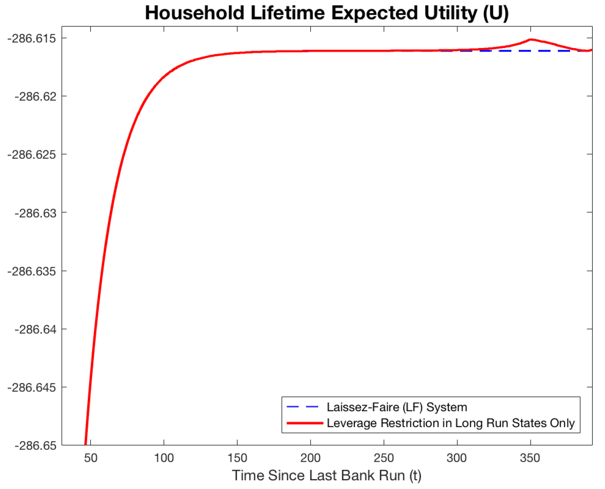
Conversely, Figure 2 presents the household’s utility under leverage restrictions in the long-run states only, relative to the laissez-faire system. If I restrict bank leverage in multiple long-run states, the household utility increases above its laissez-faire value. The plot shows a leverage restriction of 99.99% of the steady-state leverage value in the laissez-faire model, for five periods. Household utility increases under this leverage regime, relative to the baseline, implying that the benefit of decreasing the probability of a costly bank run in the long-run states more than compensates for constraining the productive bank’s ability to buy capital in these long-run periods.
In sum, the framework described in the previous section enables the assessment of leverage caps at different points of the banks’ recovery path. Consistent with Gertler et al. (2020), these results provide evidence in favor of more lenient bank leverage ratio restrictions in periods during an economic downturn, when households’ marginal utility of consumption is highest, and stricter during periods where households’ marginal utility of consumption is relatively lower. Specifically, a leverage restriction for a single period directly following the bank run can lead to a permanent decrease in utility at every state, while a multiple-period restriction in the long-run states leads to the same or better welfare at every state.

3.2. System Dynamics Under Multi-Period Leverage Restriction

In this section, I study the effects of an exogenous leverage requirement that restricts the maximum amount of leverage that bankers can choose for all periods where bankers’ total assets are greater than 15 times net worth in the uncapped laissez-faire regime. In other words, the leverage cap binds when leverage is 15 times equity or larger; these are the periods following the bank run when leverage is highest.
This leverage restriction is inspired by the U.S. Supplementary Leverage Ratio (SLR)—proposed in 2013 (and approved to be recalibrated in 2025) by the U.S. Federal Reserve, Federal Deposit Insurance Corp. (FDIC), and the Office of the Comptroller of the Currency. The SLR targeted a 6% equity-to-assets ratio for globally systemically important depository banks to be considered well-capitalized. Certain off-balance sheet exposures, partially responsible for institutions’ failures during the GFC, are explicitly included in the leverage calculation utilized by the SLR. Taking the reciprocal of 15 times assets-to-equity corresponds to 6.67% equity-to-assets. This number is only slightly more conservative than the SLR, and the model in this paper best corresponds to a non-risk-based leverage ratio, like the SLR, since there is only one type of capital asset in the model. Understanding the dynamics at play under the leverage cap—and when it ceases to bind more than the participation constraint—is instructive to understand how economic variables respond under this type of leverage restriction.
The leverage restriction I use requires that the amount of deposits banks take on be the minimum of either 90% of leverage in the laissez-faire regime or the maximum amount of leverage allowed by the incentive constraint. In this calibration of the model, the economy reaches leverage of 15 or lower—the leverage cap ceases to bind more than the participation constraint—after period 67 or 16.75 years. The economy reaches the steady state in about 120 periods or 30 years. The 16.75-year “phase-in” is akin to the 12-year phase-in, temporary exemption of assets, and recalibration of the SLR from 2013 to 2025.
I restrict leverage at 90% of the laissez-faire value in periods where it would otherwise exceed 6.67%. Following a run, the high values of leverage—which decline over time—are necessary because all banks exit and the sector must rebuild from very low net worth—a pattern consistent with reality. For example, after the Global Financial Crisis, several dealer-banks failed, leaving fewer dealer-banks to intermediate all assets, increasing their leverage to high levels. Consistently, the SLR has taken almost a decade to phase in following the GFC and is relaxed in times of crisis, consistent with banks needing to increase leverage to rebuild the economy during crises.

3.2.1. Effect of Multi-Period Leverage Restriction on Economic Variables

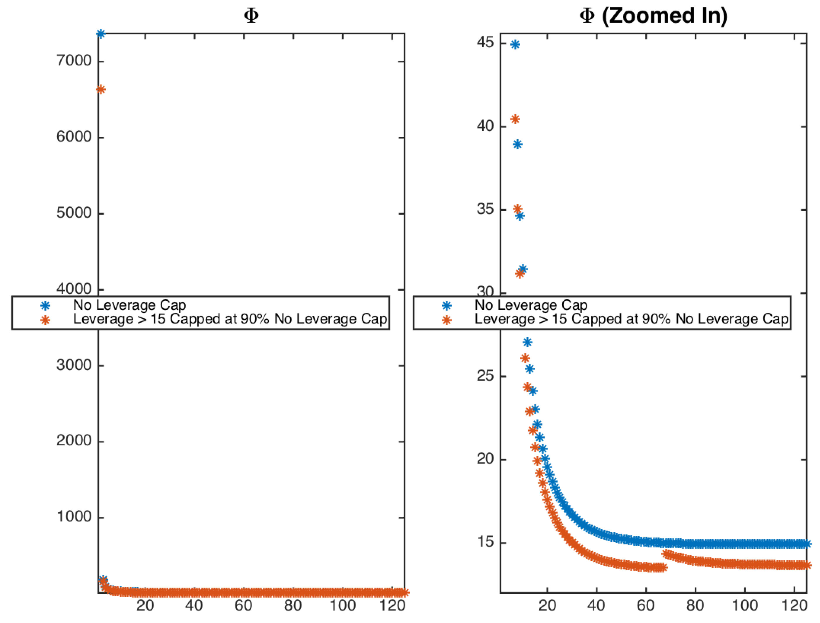
Figure 3 illustrates the recovery path that bank leverage in the economy, ϕ t , follows both with and without the leverage restriction in place. The figure on the right-hand side is a zoomed-in version that omits the first periods directly following a bank run, since these periods have enormous leverage. For all plots in this section, the x-axis denotes t or the number of periods since the last bank run. The first period, t = 1 , is the period in which the bank run occurs, and the plots illustrate the recovery path that the variable follows from the bank run period to the steady state value ( t = 120 ) . In the plots, I compare the path that the variables follow in the unrestricted model versus the path that they follow in the restricted model. Each period, there is a probability p t that a bank run occurs; however, the plots reflect the variable’s trajectory in the case that no subsequent bank run occurs before the economy reaches a steady state.
Figure 4 plots the path that the probability of a bank run, p t , follows from the time of a bank run in period one to steady state. The probability of a bank run p t decreases in the capped model relative to the uncapped model for the first 67 periods. As seen in the formula for p t , the drop in p t relative to the unrestricted system in the first 66 periods is driven by the decrease in leverage ϕ t .
p t = 1 min ( Z t + 1 + Q t + 1 * ) ( 1 K t h ) ( ϕ t 1 ) N t R t + 1 Recovery Rate , x t + 1 , 1
There is a feedback loop at work via the recovery rate. The probability of a bank run is inversely related to the recovery rate x t + 1 . The recovery rate depends not only on leverage but also on the price that capital takes on in the bank run period Q t + 1 * . During periods of extremely high leverage following the bank run, the changes in the leverage ratio dominate the effect on p t . However, for periods where the leverage ratio is close to its steady state value, changes in the bank-run price of capital dominate changes in p t . It is by taking on more leverage that banks can purchase more capital and drive up the price of capital. Therefore, forcing banks to take on lower leverage initially after a bank run can inadvertently depress the price of capital to the point that the probability of a bank run increases in the steady state.
The first term in the minimum operator is the recovery rate or the total value of bank assets in the bank-run state divided by the total cost of deposits that a bank would owe in the bank-run state. The recovery value is driven up as the leverage cap forces banks to take fewer deposits than households are willing to give them. This decreases the probability of a bank run initially, bringing it to a minimum of 0.002% in period 41 or about 10 years after the bank run, if the economy reaches that period without falling into another bank run. However, the probability of a bank run increases after the leverage cap stops binding because the cap causes irreparably low bank capital holdings while the cap binds, which drives down the price of capital in the bank-run state, Q t * , as well as the bank’s current capital holdings.
Once the leverage cap ceases to bind more than the participation constraint, banks are able to increase their net worth due to higher returns on capital since prices were depressed under the cap. However, the depressed price of capital in the bank-run state drives up the steady state probability of a bank run, p t , tightening banker incentive constraints so that higher values of net worth do not translate into a higher franchise value. Although banks are larger under the leverage cap, they cannot restore their capital holdings to laissez-faire levels because borrowers are not willing to lend them enough deposits due to the depressed recovery rate. The recovery rate is depressed because larger bank net worth ( N t ) offsets decreased leverage ( ϕ t ) in the denominator, while the numerator falls due to the decrease in Q t * and bank capital holdings.
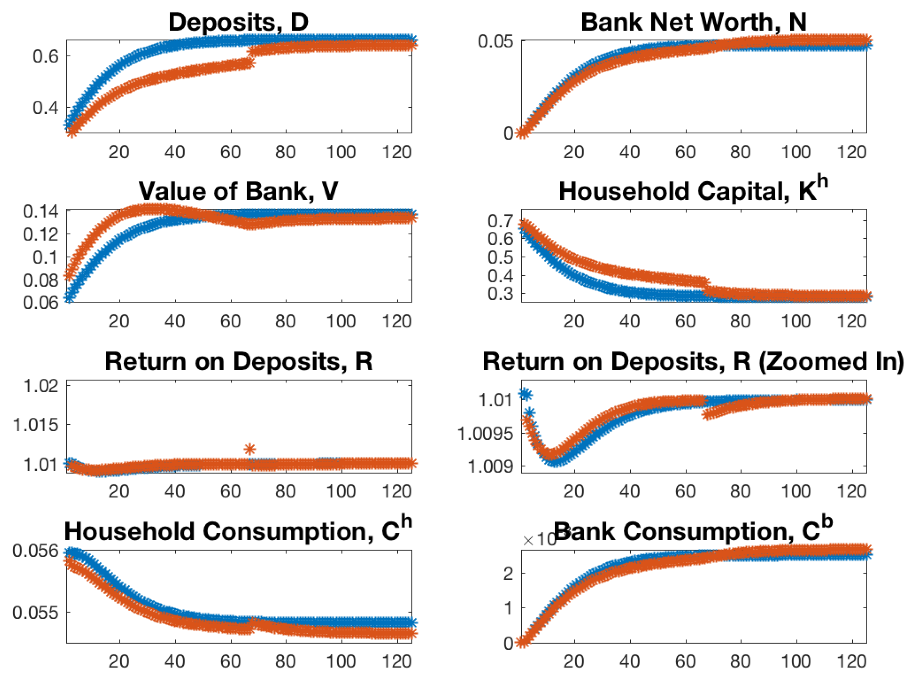
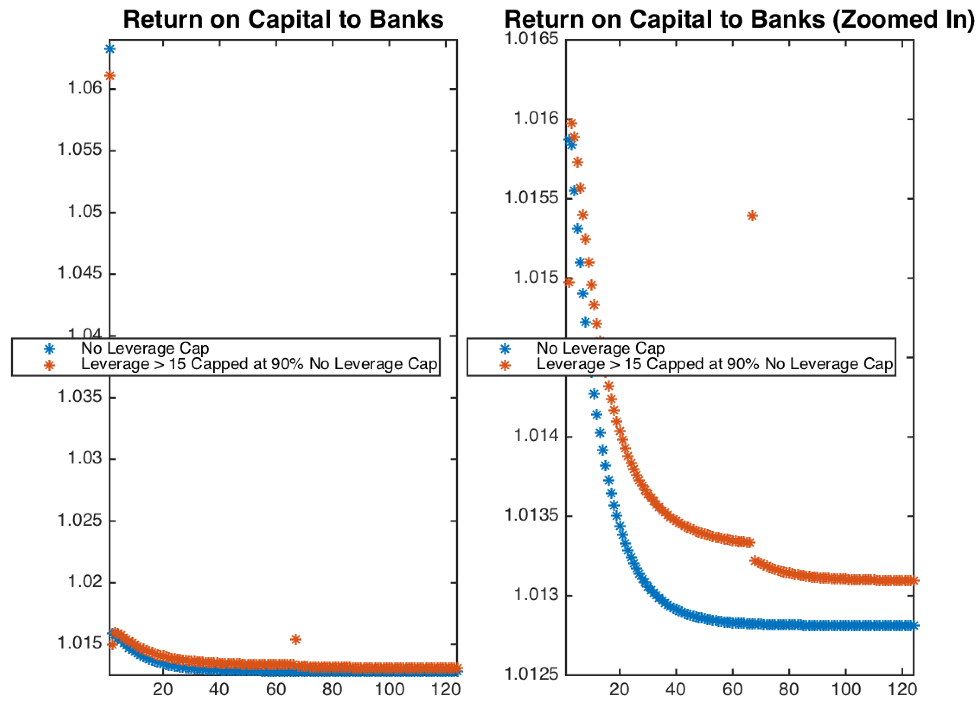
In Figure 5, return on deposits stays relatively similar between the uncapped and capped systems. For the first six periods after the bank run, the return on deposits in the capped system is lower than in the uncapped system by a maximum of 0.129 % in the period directly following the bank run, and then by about 0.004 % for the next five periods. After that, it fluctuates between very slight increases and decreases that seem to offset each other, other than a jump in the period where the leverage cap stops binding. This jump is caused by high capital returns, as well as a relative increase in the probability of a bank run as banks take on a discontinuous amount of leverage.
The banker net worth N t is mechanically equal to zero in the period after the bank run and equal to the banker’s endowment in the second period in both systems, since all existing banks are liquidated in the period that the bank run occurs, and banks in the period following the bank run enter with net worth equal only to their endowment. From periods 2 to 67, banks have a smaller net worth in the capped system by, on average, 0.0023 over this time period. However, once the leverage cap ceases to bind more than the participation constraint, banks in the capped system begin increasing their net worth relative to the uncapped system and have a net worth that is greater than the capped system by 0.0029 in the steady state.
When the leverage is capped, bankers are not allowed to take on as many deposits as households are willing to give to them based on their participation constraint. Since bankers are financially constrained, the households must directly hold the capital themselves. This leads to households holding more capital in the capped model than they do in the uncapped model. From periods 1 to 67, households hold on average 0.0835 units, or 22% more capital in the capped system than they do in the uncapped system. From periods 68 to 120, they hold on average 0.0107 units, or 3.8 % more capital, and in steady state, they hold 0.0042 units, or 1.5 % more capital.
The household’s first order condition in part helps determine the price of capital, Q t , when the household is holding any units of capital.
1 = E t ( 1 p t ) β Λ Z t + 1 + Q t + 1 Q t + f ( K t h ) + p t β Λ * Z t + 1 + Q t + 1 * Q t + f ( K t h )
where Λ * = C t h C + 1 h * is the household’s intertemporal marginal rate of substitution, conditional on a bank run occurring at time t + 1 and f ( K t h ) = α K t h . The market price of capital tends to decrease in household capital, K t h holdings, since the household’s management cost for operating capital increases with household capital holdings.
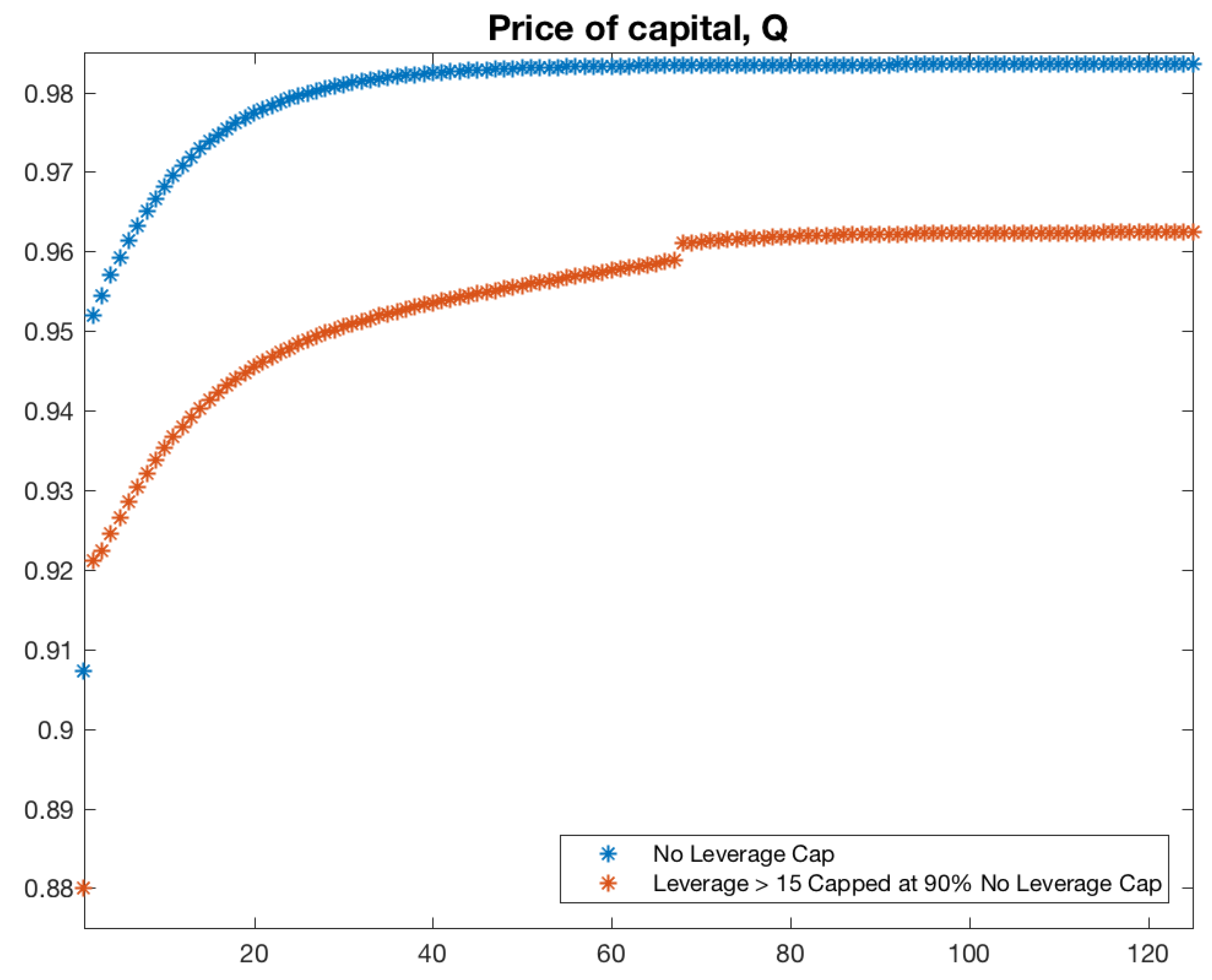
As seen in Figure 6, relative to the system with no leverage cap, the price of capital Q t is depressed along the economy’s entire recovery path after a bank run and remains depressed in steady state. In the system with capped leverage, the price of capital during a bank run is depressed to 0.88, a decrease of 3% from its laissez-faire value of 0.9072. While the leverage cap is in place, from periods 2 through 67, the price of capital is depressed by 3% on average. After the cap is no longer binding, the price of capital remains depressed by 2% on average, and stays depressed by 2% in the steady state.
This is because, in the bank run period, all banks are liquidated, so their net worth drops to zero. Once a bank has zero net worth, the assumed financial friction that net worth increases only through retained earnings (not equity injections) implies that the bank will never have a non-zero net worth at any time in the future. Therefore, in the period following the bank run, only the bankers who enter in that period will have non-zero net worth. These banks are lucky to be born at this time. They enter the economy at a time when the households hold all of the capital in the economy. Since households have a convex and increasing management cost associated with operating the capital, the households’ management costs are at their maximum. In the laissez-faire regime, the entering bankers are therefore able to extract the total surplus from their advantage in operational efficiency in the form of the highest possible returns on bank capital. These high returns increase the bankers’ value functions, loosening their participation constraints because the households are willing to lend them a lot of money to take advantage of these high returns. These very highly levered periods following a bank run are crucial to allow bankers to purchase as much capital as possible.
Capping leverage in period one decreases the amount of capital that banks are able to purchase from households. Therefore, the households hold relatively more capital and have higher management costs than in the uncapped system. Since households demand similar returns to the uncapped system, the current price of capital decreases as f ( K t h ) in their first order condition rises. This mechanism causes returns to fall for the first two periods after a bank run relative to the uncapped model, since the price at which entering bankers purchase the capital in the period following the bank run is the same in both models. However, beginning in the fourth period, the period returns in the capped system begin to surpass those in the uncapped system. This is because of the convex management costs that households shoulder as they operate more capital. As the leverage cap regime bears on, each period the banks are able to purchase less capital from the households, leaving households to operate incrementally more capital each period than they would in the laissez-faire system. The difference in returns between the capped and uncapped systems in Figure 7 reflects the convexity of the management cost. Since the households hold more capital in the capped model than they would in the uncapped model, prices are depressed, and the bankers in the capped system are able to purchase the capital at a lower price and extract rents from their advantage in operating efficiency for longer than they would be able to in the uncapped model.
Once the leverage cap ceases to bind more than the participation constraint, the banks take on the maximum amount of leverage that their participation constraint allows. This causes bank returns to jump discontinuously as the banks buy capital relatively cheaply and drive up the price of Q t discontinuously in this period. This, coupled with returns elevated from the laissez-faire level, drives up bank net worth. However, the increase in net worth relative to the uncapped level does not translate into higher capital holdings by the banks because the higher net worth and depressed price of capital in a bank-run state decrease the recovery value, increasing p t . This increase in p t decreases the banker value function and tightens banker participation constraints relative to the uncapped model. Therefore, even though the banks are slightly bigger, they cannot take on enough leverage to buy as much capital from the inefficient households as in the model with no leverage caps.
The banker’s value function is the sum of all future consumption discounted by the banker’s discount rate, as well as the probability that the banker reaches a given period. Wrapped into this probability that a banker reaches a given period is the probability that there is no bank run in that given period. In steady state, the banker net worth under the leverage cap increases slightly. However, the probability of a bank run increases as the depressed Q t * and bank capital holdings dominate the beneficial effect of decreased leverage and higher net worth in the recovery rate x t + 1 .
The increase in p t increases the discount rate on future values of banker consumption, lowering the bankers’ value function, tightening the participation constraint, and decreasing the amount of deposits that households will lend them. Therefore, even though banker net worth is increasing, the households operate elevated levels of capital, which directly leads to decreased capital prices throughout the entire recovery path. These results imply that the leverage cap introduces a wedge in the economy that allows steady state banks to be bigger and generate higher returns. However, because banks in the capped system never acquire as much leverage as in the uncapped system, they cannot purchase the lassez-faire fraction of capital. The wedge therefore forces the inefficient households to operate elevated levels of capital and allows the efficient banks to extract higher operating rents from them each period.
These dynamics suggest that leverage restrictions can enhance financial stability by lowering run risk, but at the cost of reduced capital allocational efficiency. When the cap is relaxed—such as when certain assets are exempted under the SLR or the constraint is loosened through SLR recalibration—the model predicts a discontinuous jump in leverage, a sharp increase in the probability of a bank run, and a rise in the price of capital, though not necessarily to laissez-faire levels. The model also implies that banks under the capped system will be larger. The larger banks are needed to maintain reasonable levels of capital operated by productive users since the leverage restriction hinders small, efficient banks from operating with a lot of capital.

3.2.2. Implications for Economic Stability

I simulate the economy for 10,000 periods under both the leverage cap regime in Section 3.2.1 and an uncapped baseline. In each case, the economy starts in the period following a bank run and evolves along its recovery path as solved above. Each period, a bank run occurs with probability p t . If a run occurs, the economy resets to the start of the recovery path, regardless of its prior position, and progresses sequentially toward steady state until the next run. The simulation draws a uniform random number each period to determine whether a run occurs ( < p t ) or recovery continues ( p t ) . Banks in period one have zero net worth, so their participation constraint prevents deposit-taking, implying p 2 = 0 . From period three onward, p t > 0 but decreases with time since the last run, making the economy most fragile immediately after a crisis. This process can produce multiple rapid-succession runs, significantly prolonging recovery.
After simulating both the capped and uncapped economies, I compute three statistics reported in Table 1: the average time between bank runs, the average time the economy remains in steady state once reached, and the average recovery time after a run. In the uncapped model, runs occur every 81.3 periods (20.3 years) on average, versus 109.9 periods (27.5 years) with a cap. The cap shortens recovery by about 44.2 periods (11 years) due to a lower p t while the cap binds. Conditional on reaching steady state, however, the system with the leverage cap falls out of the steady state into a bank run on average 1.3 years, or 5.2 periods, earlier than it would without a leverage cap. This is due to an elevated p t , which is caused by decreased bank-run-price of capital resulting from early allocational efficiency losses in the capped leverage system. These findings suggest that leverage caps can improve stability but, if too restrictive immediately after a crisis, may slow long-term recovery.

4. Conclusions

This paper develops a method for analyzing the welfare effects of bank leverage restrictions over the business cycle in a general equilibrium setting. The approach expresses the steady state values of household lifetime utility and bankers’ value functions, allowing each to be iterated backward using the model’s laws of motion. This backward-induction procedure enables the direct solution of the bankers’ problem under restricted leverage. Applying the method, I compare alternative leverage regimes—examining dynamics when leverage restrictions are imposed or removed, their effects on economic variables, and implications for financial stability.
A key contribution of this paper is a framework for evaluating how economic outcomes respond to dynamic macroprudential policies, such as time-varying or temporary leverage restrictions. This model allows the evaluation of the economic impact of pausing the leverage restriction or changing it mid-leverage regime. For example, the model could be used to study the relaxation of the Supplementary Leverage Ratio to increase financial intermediation during COVID, and the ratio’s proposed recalibration in 2025. The model can also be extended to evaluate the welfare effects of related interventions, including the bankruptcy treatment of repo collateral.
The results show that when the leverage restriction is binding, banks accumulate net worth more slowly, inefficient households are forced to hold more capital directly, and the price of capital remains persistently depressed. When the leverage restriction ceases to bind, banks experience a discontinuous jump in both leverage and the returns they can generate on the depressed price of capital. However, the depressed bank-run capital price leaves the steady-state run probability higher than in the laissez-faire regime. Banks under the leverage restriction end up slightly larger, although they cannot restore capital holdings to laissez-faire levels due to the inability to take on sufficient leverage.
The results highlight a central trade-off. High post-crisis leverage accelerates capital reallocation to efficient banks, raising production and household welfare, but at the cost of greater near-term run risk. Quantitative simulations show that time-varying leverage restrictions reduce the frequency of bank runs but slow recovery. These findings highlight a key tradeoff: stricter leverage restrictions lower run risk during recovery but slow post-crisis rebuilding and can depress welfare and raise long-run bank run risk relative to the laissez-faire economy. The welfare-enhancing leverage restriction is time-varying—it should loosen when household marginal utility is high and tighten as it approaches steady state.

Funding

This research received no external funding.

Institutional Review Board Statement

Not applicable.

Informed Consent Statement

Not applicable.

Data Availability Statement

This manuscript relied only on simulated data as described in the main text.

Acknowledgments

I thank Larry Christiano, Guido Lorenzoni, Dimitris Papanikolaou, Husnu Dalgic, Andrea Modena, the seminar participants at Kellogg Northwestern, Northwestern Macroeconomics, and the Federal Reserve Board for their helpful comments. Any errors in this manuscript are my own.

Conflicts of Interest

The author declares no conflicts of interest.

Notes

1
Press Release, Basel Committee on Banking Supervision, Group of Governors and Heads of Supervision announces higher global minimum capital standards (12 September 2010), http://www.bis.org/press/p100912.pdf accessed on 31 August 2025.
2
Tapia, Jose Maria, Ruth Leung, and Hashim Hamandi, “Banks’ Supplementary Leverage Ratio”, The OFR Blog, 2 August 2024. Certain off-balance sheet exposures partially responsible for institutions’ failures during the GFC are explicitly included in the SLR.
3
See, e.g., Evan Weinberger, “Leverage Cap Leaves Big Banks with Unpalatable Choices”, Law360, 9 July 2013. A leverage ratio cap of 5% was proposed for the eight GSIBs insured bank holding companies, with additional surcharges to be phased in. “Fed and FDIC agree 6% leverage ratio for US Sifis”, Central Banking Newsdesk, 10 July 2013. “US Banking Regulators Propose Changes to the Enhanced Supplementary Leverage Ratio for US GSIBs”, Skadden, 8 July 2025.
4
Hamdi et al. (2023) shows that Basel III decreased bank mortgage originations and pushed banking activity toward nonbanks and Acharya (2012) argues that Basel III is fundamentally flawed but has redeeming features when combined with the Dodd Frank Act.
5
The evidence in Lewis and Padi (2025a, 2025b) suggests that micro-level frictions in credit markets (pooled pricing and servicing incentives) interact with macroprudential constraints.
6
Just prior to the Great Recession, commercial banks operated with leverage ratios near 8 and interest margins of roughly 200 basis points (e.g., Philippon, 2015). In the shadow banking system, leverage multiples ranged from very modest levels (2 or below) for hedge funds to extremely high levels for investment banks (20 to 30). However, Singh and Aitken (2010) show that repo collateral reuse increased dealer-bank leverage by 50% more than these standard estimates during 2007–2009. Interest margins ranged from 25 basis points for ABX securities to 100 or more for agency mortgage-backed securities and BAA corporate bonds.

References

  1. Acharya, V. V. (2012). The dodd-frank act and basel iii: Intentions, unintended consequences, and lessons for emerging markets (ADBI Working Paper, Tech. Rep.). ADBI. [Google Scholar]
  2. Acharya, V. V., Gale, D., & Yorulmazer, T. (2011). Rollover risk and market freezes. The Journal of Finance, 66(4), 1177–1209. [Google Scholar] [CrossRef]
  3. Arfaoui, J., & Uhlig, H. (2025). Maturity risks and bank runs (Tech. Rep.). National Bureau of Economic Research. [Google Scholar]
  4. Begenau, J. (2020). Capital requirements, risk choice, and liquidity provision in a business-cycle model. Journal of Financial Economics, 136(2), 355–378. [Google Scholar] [CrossRef]
  5. Bernanke, B. S., Gertler, M., & Gilchrist, S. (1999). The financial accelerator in a quantitative business cycle framework. Handbook of Macroeconomics, 1, 1341–1393. [Google Scholar]
  6. Christiano, L., Dalgic, H., & Li, X. (2022). Modelling the Great Recession as a Bank Panic: Challenges. Economica, 89, S200–S238. [Google Scholar] [CrossRef]
  7. Christiano, L., & Ikeda, D. (2016). Bank leverage and social welfare. American Economic Review, 106(5), 560–564. [Google Scholar] [CrossRef]
  8. Cole, H. L., & Kehoe, T. J. (2000). Self-fulfilling debt crises. The Review of Economic Studies, 67(1), 91–116. [Google Scholar] [CrossRef]
  9. De Nicolò, G., Gamba, A., & Lucchetta, M. (2014). Microprudential regulation in a dynamic model of banking. The Review of Financial Studies, 27(7), 2097–2138. [Google Scholar] [CrossRef]
  10. Diamond, D. W., & Dybvig, P. H. (1983). Bank runs, deposit insurance, and liquidity. Journal of Political Economy, 91(3), 401–419. [Google Scholar] [CrossRef]
  11. Ennis, H. M., & Keister, T. (2010). Banking panics and policy responses. Journal of Monetary Economics, 57(4), 404–419. [Google Scholar] [CrossRef]
  12. Gertler, M., & Kiyotaki, N. (2015). Banking, liquidity, and bank runs in an infinite horizon economy. American Economic Review, 105(7), 2011–2043. [Google Scholar] [CrossRef]
  13. Gertler, M., Kiyotaki, N., & Prestipino, A. (2020). Credit booms, financial crises, and macroprudential policy. Review of Economic Dynamics, 37, S8–S33. [Google Scholar] [CrossRef]
  14. Goldstein, I., & Pauzner, A. (2005). Demand–deposit contracts and the probability of bank runs. The Journal of Finance, 60(3), 1293–1327. [Google Scholar] [CrossRef]
  15. Gorton, G., & Metrick, A. (2012). Securitized banking and the run on repo. Journal of Financial Economics, 104(3), 425–451. [Google Scholar] [CrossRef]
  16. Gorton, G., & Ordonez, G. (2020). Good booms, bad booms. Journal of the European Economic Association, 18(2), 618–665. [Google Scholar] [CrossRef]
  17. Hamdi, N., Jiang, E. X., Lewis, B. A., Padi, M., & Pal, A. (2023). The rise of nonbanks in servicing household debt. Olin business school center for finance & accounting research paper 2023/08. Available online: https://ssrn.com/abstract=4550175 (accessed on 31 August 2025).
  18. He, Z., & Krishnamurthy, A. (2012). A model of capital and crises. The Review of Economic Studies, 79(2), 735–777. [Google Scholar] [CrossRef]
  19. Kiyotaki, N., & Moore, J. (1997). Credit cycles. Journal of Political Economy, 105(2), 211–248. [Google Scholar] [CrossRef]
  20. Lewis, B. A. (2021). The impact of collateral value on mortgage originations. Olin business school center for finance & accounting research paper no. 2023/04. Available online: https://ssrn.com/abstract=4423818 (accessed on 31 August 2025).
  21. Lewis, B. A. (2023). Creditor rights, collateral reuse, and credit supply. Journal of Financial Economics, 149(3), 451–472. [Google Scholar] [CrossRef]
  22. Lewis, B. A., & Padi, M. (2025a). Regulating secondary loan markets: Evidence from small business lending. Olin business school center for finance & accounting research paper (2025/01). Available online: https://ssrn.com/abstract_id=5187744 (accessed on 31 August 2025).
  23. Lewis, B. A., & Padi, M. (2025b). The cost of servicing debt pools. Available online: https://ssrn.com/abstract=5386507 (accessed on 31 August 2025).
  24. Martinez-Miera, D., & Suarez, J. (2014). Banks’ endogenous systemic risk taking. Manuscript, CEMFI, 42. Available online: https://martinezmiera.com/wp-content/uploads/2016/02/mmiera-suarez2014.pdf (accessed on 31 August 2025).
  25. Morris, S., & Shin, H. S. (1998). Unique equilibrium in a model of self-fulfilling currency attacks. American Economic Review, 88, 587–597. [Google Scholar]
  26. Nguyen, T. T. (2015). Bank capital requirements: A quantitative analysis. Charles A. Dice center working paper 2015-14. Available online: https://ssrn.com/abstract=2356043 (accessed on 31 August 2025).
  27. Philippon, T. (2015). Has the US finance industry become less efficient? On the theory and measurement of financial intermediation. American Economic Review, 105(4), 1408–1438. [Google Scholar] [CrossRef]
  28. Roe, M. J. (2010). The derivatives market’s payment priorities as financial crisis accelerator. Stanford Law Review, 63, 539. [Google Scholar] [CrossRef][Green Version]
  29. Singh, M. M., & Aitken, J. (2010). The (sizable) role of rehypothecation in the shadow banking system (No. 10-172). International Monetary Fund.[Green Version]
  30. Van den Heuvel, S. J. (2008). The welfare cost of bank capital requirements. Journal of Monetary Economics, 55(2), 298–320. [Google Scholar] [CrossRef]
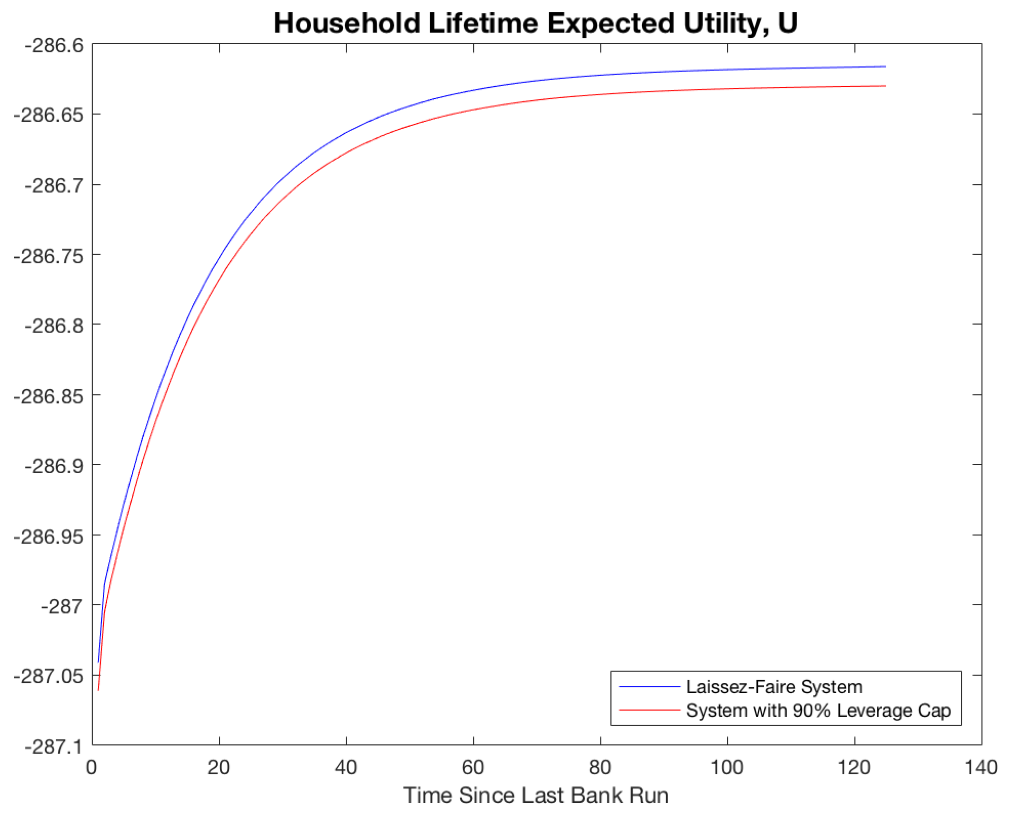
Figure 1. Household utility with 90% leverage cap in period 2 only.
Jrfm 18 00519 g001
Figure 2. Household utility with 99.99% leverage cap in the long-run states only.
Jrfm 18 00519 g002
Figure 3. Leverage ϕ t with multiple-period leverage cap.
Jrfm 18 00519 g003
Figure 4. Probability of bank run p t with multiple-period leverage cap.
Jrfm 18 00519 g004
Figure 5. Recovery path after bank run with and without multiple-period leverage cap (blue: no leverage cap, red: leverage > 15 capped at 90% no leverage cap).
Jrfm 18 00519 g005
Figure 6. Price of capital Q t with and without multiple-period leverage cap.
Jrfm 18 00519 g006
Figure 7. Return on bank assets after a bank run with and without multiple-period leverage cap.
Jrfm 18 00519 g007
Table 1. Recovery times economy simulated 10,000 periods (multi-period leverage cap).
Average Number of PeriodsNo Leverage CapLeverage Cap
Between Bank Runs81.3109.9
To Reach SS318.1273.9
In SS (Conditional on Reaching)87.182.0
Disclaimer/Publisher’s Note: The statements, opinions and data contained in all publications are solely those of the individual author(s) and contributor(s) and not of MDPI and/or the editor(s). MDPI and/or the editor(s) disclaim responsibility for any injury to people or property resulting from any ideas, methods, instructions or products referred to in the content.