Abstract
The banking system, as the most important sector of the economy of every country, often encounters a number of risks. Financial institutions of that system operate in an unstable environment, and without having complete information about that environment, they may suffer significant losses. The main source of such losses is considered to be credit risks, and for the management of these, various mathematical models are being developed which will allow banks to make decisions on granting a loan. Lately, for this purpose, machine learning (ML) classification algorithms have often been used for credit risk modeling. In this research work, using the ideas of well-known ML algorithms, a new algorithm for solving the binary classification problem was developed. By means of the algorithm created, based on real data, a classification model has been developed. Qualitative indicators of that model, such as ROC AUC, PR AUC, precision, recall, and F1 score, were evaluated. By modifying the resulting probabilities into a range of 300–850 score points, a scoring model has been developed, the usage of which can mitigate credit risk and protect financial organizations from major losses.
1. Introduction
Historically, proper credit risk management has played a key role in the normal functioning of the economy and in the prevention of financial crises (Chen et al., 2016). For example, the global financial crisis of 2008 highlighted the importance of precise credit risk management. The Basel Committee on Banking Supervision also emphasizes the active and coordinated management of this type of risk, which contributes to the stability of the banking system (Basel Committee on Banking Supervision, 2010, 2015).
At the time of lending, credit organizations often apply various developed models in order to assess the credit risk of an individual—for example, the FICO (Fair Isaac Corporation) scoring model (Addo et al., 2018). FICO credit scoring solutions provide a better understanding of credit risk in lending to consumers and businesses. The introduction of broad-based credit scores by FICO more than 30 years ago has transformed economic growth in the US and globally, making access to credit more efficient and objective while protecting the financial stability of lenders by enabling decisions that limit risk (Alabi & Bukola, 2023).
This model and its analogs are “black boxes”, and credit organizations often cannot clearly understand the reason for the formation of this or that score point. Moreover, these models are often built based on the data of borrowers from only few countries and, in essence, do not describe the social–economic situation of the operation region of a credit organization. For the same reasons, for accurate evaluation and credit risk management, credit organizations often collect information on their borrowers and the quality of the loans provided themselves, and based on all that data, they build models (Addo et al., 2018). Historically, logistic regression models are used often in order to solve such problems. However, recently, it has been noted that modern ML models are often also used in order to solve this problem, for example, XGBoost, LightGBM, Neural Network, etc. (Pinheiro et al., 2025).
The aim of this research work is to investigate the behavior of borrowers based on real data, applying the ideas of known ML models to develop new algorithms for solving binary classification problems. During the study, a comparative analysis of the proposed classification algorithm was carried out with other machine learning algorithms such as logistic regression, kNN and XGBoost.
The aim is also to develop a local score system of the given bank based on the data of the borrowers available to us by using new algorithms.
The results of this research can be used by credit organizations, which will contribute to the optimal credit risk management and to cost reduction in the given organizations.
2. Literature Review
Many scientific works by others have been considered within the framework of this research. We shall consider some of them.
Montevechi et al. (2024) conducted a comprehensive review of credit risk modeling with machine learning, emphasizing the importance of loan granting as a central part of banking operations and the associated credit risks. The study analyzed the strengths and weaknesses of ML methods, data preprocessing, variable selection, model optimization, and other critical phases. The authors concluded that ML implementation in financial risk management is increasing; however, standardized modeling procedures are necessary before complex classifiers can be commercially deployed.
Noriega et al. (2023) conducted a systematic literature review on credit risk prediction using machine learning, emphasizing the importance of AI and ML adoption by financial institutions to evaluate credit risk from large datasets. Their analysis of popular databases identified 52 studies related to the microfinance lending sector. The review showed that boosted models are the most frequently studied ML approaches, and common evaluation metrics include Area Under the Curve (AUC), Accuracy (ACC), Recall, F1-score, and Precision.
Chang et al. (2024) investigated credit card default prediction using multiple machine learning models, including neural networks, logistic regression, AdaBoost, XGBoost, and LightGBM. Their results indicate that XGBoost outperforms the other models, achieving 99.4% accuracy, and that the application of ML and deep learning (DL) algorithms significantly improves forecast accuracy for customer defaults. However, while many different types of algorithms are mentioned in this study, the authors do not provide detailed explanations of what these algorithms are, how they operate, or how they differ from one another. For instance, logistic regression is a traditional statistical model focusing on linear relationships, whereas neural networks belong to deep learning approaches that capture complex, nonlinear patterns. Ensemble methods such as AdaBoost, XGBoost, and LightGBM, on the other hand, combine multiple weak learners (usually decision trees) to improve predictive performance, but differ in terms of boosting strategy, speed, and regularization techniques. Without clarifying these distinctions, the comparative insights remain somewhat superficial, making it difficult for practitioners and researchers to fully grasp why certain algorithms outperform others in the credit risk domain.
Shi et al. (2022) conducted a systemic review of 76 studies published over the last eight years, focusing on credit risk assessment using statistical, machine learning (ML), and deep learning (DL) methods. They proposed a new classification methodology for ML-based credit risk algorithms and ranked their efficiency. The study demonstrated that deep learning models generally outperform statistical ML algorithms, and that ensemble methods—which combine the predictions of multiple models (e.g., decision trees or neural networks) to produce a more robust and accurate outcome—achieve higher accuracy than individual models. It is also important to note that most of the reviewed studies focus on asset classes with abundant historical data, such as retail loans, credit cards, and SMEs, whereas low-default portfolios, such as large corporates and sovereigns, are less frequently studied due to insufficient default events, limiting the applicability of ML approaches in these segments.
Mhlanga (2021) examined the application of machine learning (ML) and artificial intelligence (AI) in credit risk assessment within emerging economies. The study found that ML and AI significantly improve credit risk evaluation by leveraging diverse data sources, enabling lenders to gain deeper insights into borrower behavior. The author recommends that financial organizations invest in AI and ML technologies to enhance risk assessment processes.
Alagic et al. (2024) analyzed loan approval prediction by integrating data on borrowers’ mental health. Using a dataset of 1991 individuals, the study demonstrated that selected machine learning (ML) algorithms—chosen based on their prior performance in similar classification tasks and their suitability for handling mixed data types—can effectively distinguish between high-risk and low-risk customers. This approach highlights the importance of carefully selecting ML algorithms to ensure accurate predictions in credit risk assessment.
Guan et al. (2023) explored responsible credit risk assessment by combining machine learning (ML) algorithms with human knowledge acquisition. The study applied ML models to a small dataset, then corrected data errors using human expertise through Ripple-Down Rules (RDR), a method for incrementally updating decision rules to fix errors without retraining the entire model. The results showed that the combined model trained on limited data performed comparably to models trained on larger datasets. This approach is versatile and can enhance the validity of lending decisions.
Suhadolnik et al. (2023) conducted an empirical evaluation of ten machine learning (ML) models using over 2.5 million observations. Their results indicate that ensemble models, particularly XGBoost, outperform traditional algorithms such as logistic regression in terms of predictive performance. Logistic regression is a classical statistical model that estimates the probability of default based on linear relationships between predictors, while XGBoost is a gradient-boosted decision tree algorithm that iteratively combines weak learners to achieve stronger predictive accuracy. Unlike single models, ensemble approaches such as XGBoost reduce overfitting and capture nonlinear interactions more effectively, which explains their superior performance.
Bulut and Arslan (2024) investigated the impact of dimensionality reduction and data splitting on classification performance in credit risk assessment. Using principal component analysis (PCA), the dataset of 20 features was reduced to 13 principal components (PCs). A PC is a new uncorrelated variable created as a linear combination of the original correlated features, capturing as much of the original data’s variance as possible. PCA is a statistical technique that transforms correlated variables into a smaller set of uncorrelated components, retaining most of the variance while reducing noise and redundancy. The study applied Random Forest, Logistic Regression, Decision Tree, and Naive Bayes algorithms. Random Forest and Decision Tree are tree-based models, with the former using an ensemble of multiple trees to improve stability and accuracy, while Logistic Regression is a linear classifier, and Naive Bayes is a probabilistic model based on conditional independence. Their findings showed that models trained on the reduced dataset performed as well as or better than those trained on the original dataset, highlighting the importance of feature reduction for efficiency without sacrificing predictive power.
Trivedi (2020) examined credit score modeling using various feature selection methods and machine learning (ML) algorithms. Using available credit data from Germany, the study demonstrated that forecast accuracy can be improved by selecting the optimal combination of variable selection methods and ML models. The analysis identified Random Forest combined with Chi-Square feature selection as the most effective approach.
To summarize the reviewed studies, in the scientific world, various research methods are often studied, and in practical model building, known ML models are used. For that reason, the results of the current research are even more up to date.
3. Research Methodology
Within this research, various data processing methods were used. To identify patterns in the data, correlation analysis was used, namely the Pearson correlation coefficient, because the numeric variables being analyzed are continuous and approximately normally distributed, which allows for the assessment of linear relationships in the dataset.
Correlation is a bivariate analysis that measures the strength of association between two variables and the direction of the relationship (Suhadolnik et al., 2023). This coefficient shows a linear relationship between variables.
Taking into account that the dataset contains categorical variables, the data was processed using the One Hot Encoding method, which is a method for converting categorical variables into a binary format. It creates new binary columns (0 s and 1 s) for each category in the original variable. Each category in the original column is represented as a separate column, where a value of 1 indicates the presence of that category and 0 indicates its absence (Lee et al., 2022).
Taking into account that the dataset contains numerical variables, the data was processed using StandardScaler method.
StandardScaler is a versatile and widely used preprocessing technique that contributes to the robustness, interpretability, and performance of machine learning models trained on diverse datasets.
StandardScaler operates on the principle of normalization, where it transforms the distribution of each feature to have a mean of zero and a standard deviation of one. This process ensures that all features are on the same scale, preventing any single feature from dominating the learning process due to its larger magnitude.
In order to solve the classification problem in this research, a new binary classification algorithm was developed, which consists of the following steps mentioned below:
- Depending on the dependent variable (y), it is necessary to divide the existing dataset (S) into two subsets. The first subsets will consist of (S0) those observations, for which y takes the value of 0 and the second (S1) y takes the value of 1:where : i is the vector of the observation variable, and S is the initial dataset.
- For each subset obtained as described above, we calculate the centroid of the group using the formulas below:where and are the centroids of the choices, and and are the amounts of the relevant subsets.
- We calculate the distances from the point subject to classification to the centroid of each group, as well as to its N nearest neighbors (where N is the number of nearest points). The distance can be measured using various methods. Within the framework of this study, Euclidean distance was applied according to the formula given below (Gallet & Gowanlock, 2022):where p and q are two points in n-dimensional space. Points p and q can be either the point to be classified and the centroid of each group, or the point to be classified and one of the N nearest neighbors.
- Applying the distances obtained in point 3, we calculate the influence of each centroid and each nearest neighbor according to the formula mentioned below:where d(p, q) is the distance between points p and q. The points p and q can be the new point to be classified (p) and the nearest neighbors or the centroids (C0 and C1) of each group (q); e is a small rational number used to prevent division by zero, and k is a hyperparameter of the proposed model, determined during model training.
- The probability of the point subject to classification belonging to the class 0 or 1 is calculated according to the formulas given below:where and are the influence of class centroids 0 and 1, and are the influences from a given point to the N nearest neighbors (0 and 1 class neighbors), and Probability(0) and Probability(1) are the probabilities of belonging to groups 0 and 1 of the point subject to classification (Figure 1).
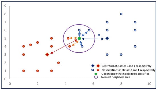 Figure 1. Classification algorithm diagram.
4. Analysis
The study is based on real credit information regarding consumer loans to individuals, using data from Unibank OJSC. The variables were selected based on (i) their availability in the bank’s credit information system, (ii) their proven relevance in prior research on credit risk assessment, and (iii) consultations with domain experts at Unibank OJSC. These variables capture key dimensions of borrower characteristics (e.g., demographic and financial indicators) and loan contract conditions, which are known to strongly influence default risk.
In this dataset, there are 13 variables:
- Education. In the original data, this variable had the values E1, E2, E3, and E4. Each value has been changed to “Academic degree”, “Higher education”, “Medium professional”, and “High school”, respectively.
- Availability of property. In the original data, this variable had the values P1, P2, P3, and P4. Each value has been changed to “Availability of real estate”, “Availability of movable property”, “Availability of real estate and movable property”, and “Absence”, respectively.
- Borrower’s Age. This variable is numeric and contains values from 20 to 65.
- Number of days past due in the last 12 months. This variable is numeric and contains values from 0 to 1600.
- Number of delays. This variable is numeric and contains values from 1 to 67. This variable contains missing data. Based on the information received from the bank, it became clear that these clients do not have overdue debts. Based on this, the missing values were changed to 0.
- Number of changes in risk classes. This variable is numeric and contains values from 0 to 28.
- Credit load. This variable is numeric and contains values from 0 to 2,984,303. Data are presented in AMD.
- Credit history length. This variable is numeric and contains values from 0 to 488. Data is presented in days.
- Maximum repaid loans. This variable is numeric and contains values from 0 to 25,131,048. Data are presented in AMD.
- Contract sum. This variable is numeric and contains values from 30,000 to 2,300,000. Data are presented in AMD. There are some outliers in the data. These are the clients to whom the bank has issued a loan in of an amount more than AMD 1,000,000. There are seven such observations in the sample. It was calculated that the removal of observational data does not significantly affect the quality of the models. Therefore, when creating models, these observations were not removed from the dataset.
- Default. Binary data is presented: 1—default, 0—no default. Based on the information received from the bank, a default is considered the presence of overdue obligations for 90 days or more at least once in the last year.
In the dataset, there are 4603 observations. For modeling purposes, the ‘default’ variable was chosen as the dependent variable.
Both the analysis and the model building were carried out with the help of the Excel (version 2021) program and the Python (version 3.11) programming language and its appropriate libraries, which were the Pandas (2.2.3), Matplotlib (3.8.1), Seaborn (0.12.2), and Scikit-learn (2.2.3).
Descriptive statistics of the numerical variables are presented in Table 1. It can be seen that there are no omissions in the data, because there are 4603 variables in total. The statistical average for all the variables is represented in the table, along with minimum and maximum values, as well as 25%, 50%, and 75% percentiles (Marshall & Jonker, 2010).

Table 1.
Descriptive statistics.
A correlation matrix was constructed for the numerical variables (Table 2) and shows that there is a moderate connection between “Number of changes in risk classes” and “Number of delays”, “Credit history length” and “Credit load” variables. The correlations between the independent and dependent variables were assessed using the Pearson correlation coefficient (Table 2). Although individual variables show relatively low pairwise correlation with the dependent variable, they were retained for modeling because machine learning algorithms can capture nonlinear and multivariate interactions that are not apparent from simple correlation analysis.
Table 2.
Correlation analysis.
Within the framework of this research work, various variables were analyzed which showed that default is evident in the age group of 20–25 (50.49%, Table 3, Figure 2), as well as in the group of customers that have real estate (44.36%, Table 4, Figure 3) and in the group of customers that have medium professional education level (42.83%, Table 5, Figure 4).
Table 3.
Analysis of age groups.
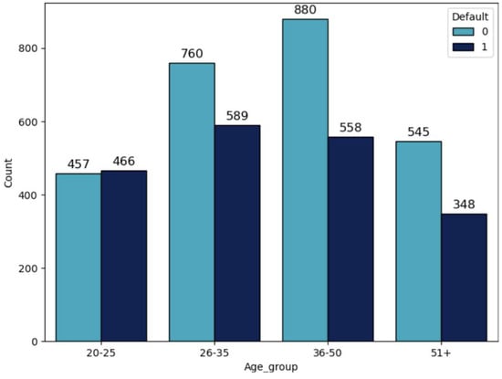
Figure 2.
Distribution by age group with division by default.
Table 4.
Analysis of customers depending on availability of property.
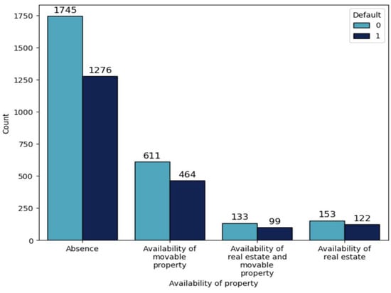
Figure 3.
Distribution by availability of property with division by default.
Table 5.
Analysis of customers depending on the level of education.
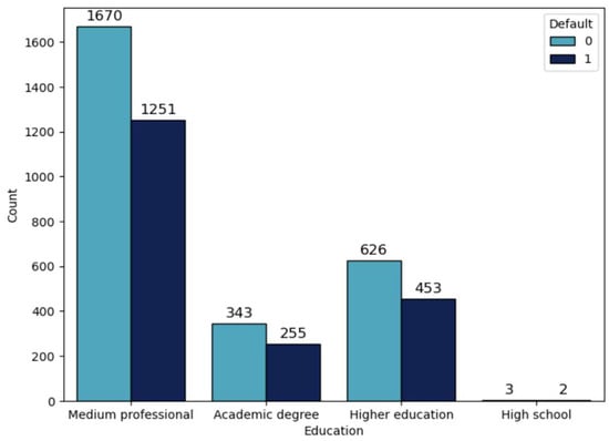
Figure 4.
Distribution by education with division by default.
Although some variables, such as age, do not show a monotonic relationship with default (Figure 2), they were retained for modeling because machine learning algorithms can capture complex, nonlinear, and non-monotonic patterns. Therefore, monotonicity was not a strict criterion for variable selection in this study.
After completing analysis, it is necessary to develop a classification model according to the methodology mentioned in this research to evaluate the qualitative indicators of that model and to modify the obtained probabilities into 300–850 score points. The predicted probabilities of default were converted to a 300–850 point scale following the standard FICO credit scoring methodology. This transformation translates raw probabilities into a familiar credit score range, making the results more interpretable for lenders and borrowers.
For modeling purposes, certain modifications were made to the existing data and are mentioned below:
- The entire dataset was divided into training (80%) and testing (20%) subsets.
- For each subset obtained in point 1—“Contract sum”, “Age”, “Credit load”, “Credit history length”, “Number of days past due in the last 12 months”, “Number of delays” and “Maximum repaid loans”—variables were standardized using the StandardScaler instrument in the Sklearn library in Python programming language (Pedregosa et al., 2011).
- For all categorical variables, dummy variables were created using the get_dummies instrument of the Pandas library in Python programming language (Pandas Development Team, 2023).
In the Section 3 of this research, the proposed methodology was implemented using Python programming language. The amount of N neighbors was chosen from the range of [58, 63], and k coefficient from the range of [−14, −1]. N was chosen to be 60, and k to be −1.0125, because that combination provided the best result for the model. The values of N (number of neighbors) and k (influence coefficient) were optimized using the Hyperopt library of the Python programming language, which is based on Bayesian optimization. During the optimization, a cross-validation strategy was applied to ensure that the choice of hyperparameters does not overfit the model.
In Figure 5, ROC and PR curves (based on the test set) and appropriate AUC coefficients are presented (Bradley, 1997).
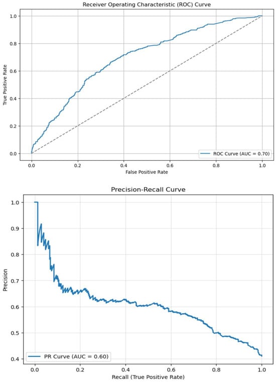
Figure 5.
ROC and PR curves.
The threshold of 0.4273 was chosen as the best threshold of the model, and in this case the accuracy was equal to 0.6678, precision was equal to 0.6098, recall was equal to 0.5291, and F1 score was equal to 0.5666. The optimal classification threshold was chosen as the probability value that maximizes the Youden statistic J = TPR − FPR on the ROC curve. This provides the best compromise between sensitivity (the ability to detect positive cases) and specificity (the ability to avoid false positives). Choosing the optimal classification threshold is important to the business because if it is chosen incorrectly, the financial company may incur serious losses in the form of issuing loans to customers who have a low creditworthiness level. In addition, the financial company may incur losses in the form of lost potential revenue due to rejecting creditworthy customers (Vallejos & McKinnon, 2013).
In Figure 6, the confusion matrix of the built model is presented, from which it is evident that the model revealed around 66% of defaults (251/378); at the same time, it refuses 186 good customers, which is around 34% (186/543) of the good customers in the test subset (Dyrland et al., 2023).
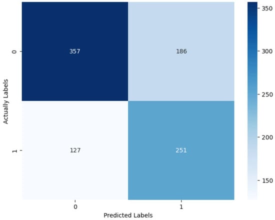
Figure 6.
Confusion matrix.
After the above, as a result of the prediction of the test subset, the probability of obtaining a 0 class was modified into score points, which could be in the range of 300–850. The modification is carried out according to the following formula:
where Score is a score point, is the probability of class 0, and and are the 1st and 99th percentiles of the logarithmic row.
In Figure 7, the distribution of the resulting score groups is presented.
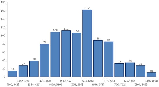
Figure 7.
Distribution of scores.
In this research work, logistic regression models, kNN and XGBoost were also constructed. The choice of these models was due to the fact that in this article, the proposed model was compared with both simple algorithms (for example, kNN) and more complex algorithms (for example, XGBoost). Considering the fact that financial companies often take logistic regression as credit scoring models, the proposed model was also compared with it. The hyperparameters of the specified models were optimized using the Hyperopt library of the Python programming language. Table 6 shows a set of hyperparameters, search ranges for the values of these hyperparameters, and the optimal value of this indicator for each model.
Table 6.
Hyperparameters of logistic regression models, kNN and XGBoost.
Table 7 presents a comparative analysis of the proposed model, the logistic regression model, kNN and XGBoost and also indicates the advantages and disadvantages of each model.
Table 7.
Comparative analysis of models.
Comparison of different classification models (logistic regression, kNN, XGBoost, and the proposed model) showed that each of them has certain advantages and limitations. Logistic regression demonstrates simplicity and interpretability, but its quality indicators remain at a lower level. The kNN algorithm achieves very high metric values on the training set, which indicates its ability to accurately adjust to the data, but a significant drop in quality on the test set indicates pronounced overfitting. The XGBoost model demonstrates high results for most metrics on the test set, but requires significantly more computing resources and has a risk of overfitting (Li et al., 2020).
Against this background, the proposed model exhibits the most stable behavior: the differences between the metrics on the training and test sets are minimal, which indicates the absence of overfitting and a high degree of generalization ability. Despite slightly lower absolute metric values compared to XGBoost, the author’s model provides balanced results across all metrics (Accuracy, Precision, Recall, F1 Score, ROC AUC, and PR AUC) and demonstrates robustness when applied to previously unseen data (Miao & Zhu, 2022). This makes it a practical and robust solution for problems where the stability and reproducibility of results are key, rather than maximizing individual metrics on a test set. Such qualities of models are necessary in credit scoring models.
5. Conclusions
It is crucial for every credit institution to properly identify and manage credit risks, and the development of reliable decision-making tools plays a key role in this process. The aim of this research was to develop and evaluate a new machine learning model for the binary classification of credit risk. Alongside the author’s model, well-established algorithms such as logistic regression, kNN, and XGBoost were implemented and compared. The results demonstrate that the proposed model achieves a favorable balance between accuracy, robustness, and reliability, which makes it an attractive option for credit organizations seeking to optimize risk assessment processes.
From a policy and managerial perspective, the findings suggest that the adoption of advanced machine learning models can enhance the stability of lending decisions, contribute to better credit portfolio quality, and support compliance with prudential risk management requirements. On the practical side, the model can be applied by financial institutions as a tool to minimize credit losses and to strengthen decision-making frameworks in day-to-day lending operations.
Nevertheless, this study has several limitations. The analysis was based on a specific dataset and did not cover all possible macroeconomic or behavioral risk factors that may influence credit default. Furthermore, the study did not address issues related to deploying models in large-scale banking environments.
In terms of future perspectives, subsequent research could extend the dataset, incorporate additional explanatory variables, and test the applicability of the model in diverse regulatory and institutional contexts. Another important direction would be the integration of such models into existing risk management systems, which would provide further insights into their practical effectiveness.
Author Contributions
Conceptualization, G.A. and A.G.; methodology, G.A. and A.G.; software, G.A.; validation, G.A.; formal analysis, G.A.; investigation, G.A.; writing—original draft preparation, G.A. and A.G.; writing—review and editing, G.A. and A.G.; visualization, G.A. All authors have read and agreed to the published version of the manuscript.
Funding
This research received no external funding.
Institutional Review Board Statement
Not applicable.
Informed Consent Statement
Not applicable.
Data Availability Statement
The data presented in this study are available on request from the corresponding author due to privacy reasons.
Conflicts of Interest
The authors declare no conflicts of interest.
References
- Addo, P. M., Guegan, D., & Hassani, B. (2018). Credit risk analysis using machine and deep learning models. Expert Systems with Applications, 134, 26–39. [Google Scholar] [CrossRef]
- Alabi, O., & Bukola, T. (2023). Introduction to Descriptive statistics. In Recent advances in biostatistics. IntechOpen. [Google Scholar] [CrossRef]
- Alagic, A., Zivic, N., Kadusic, E., Hamzic, D., Hadzajlic, N., Dizdarevic, M., & Selmanovic, E. (2024). Machine learning for an enhanced credit risk analysis: A comparative study of loan approval prediction models integrating mental health data. Machine Learning and Knowledge Extraction, 6(1), 53–77. [Google Scholar] [CrossRef]
- Basel Committee on Banking Supervision. (2010). Principles for enhancing corporate governance. Bank for International Settlements. Available online: https://www.bis.org/publ/bcbs176.pdf (accessed on 10 September 2025).
- Basel Committee on Banking Supervision. (2015). Corporate governance principles for banks. Bank for International Settlements. Available online: https://www.bis.org/bcbs/publ/d328.pdf (accessed on 10 September 2025).
- Bradley, A. P. (1997). The use of the area under the ROC curve in the evaluation of machine learning algorithms. Pattern Recognition, 30(7), 1145–1159. [Google Scholar] [CrossRef]
- Bulut, C., & Arslan, E. (2024). Comparison of the impact of dimensionality reduction and data splitting on classification performance in credit risk assessment. Artificial Intelligence Review, 57(9), 252. [Google Scholar] [CrossRef]
- Chang, V., Sivakulasingam, S., Wang, H., Wong, S. T., Ganatra, M. A., & Luo, J. (2024). Credit risk prediction using machine learning and deep learning: A study on credit card customers. Risks, 12(11), 174. [Google Scholar] [CrossRef]
- Chen, N., Ribeiro, B., & Chen, A. (2016). Financial credit risk assessment: A recent review. Artificial Intelligence Review, 45, 1–23. [Google Scholar] [CrossRef]
- Dyrland, K., Lundervold, A. S., & Porta Mana, P. G. L. (2023). Does the evaluation stand up to evaluation? A first-principle approach to the evaluation of classifiers. arXiv, arXiv:2302.12006. [Google Scholar] [CrossRef]
- Gallet, B., & Gowanlock, M. (2022). Leveraging GPU tensor cores for double precision Euclidean distance calculations. arXiv, arXiv:2209.11287. [Google Scholar] [CrossRef]
- Guan, C., Suryanto, H., Mahidadia, A., Bain, M., & Compton, P. (2023). Responsible credit risk assessment with machine learning and knowledge acquisition. Human-Centric Intelligent Systems, 3(3), 232–243. [Google Scholar] [CrossRef]
- Lee, Y., Park, C., & Kang, S. (2022). Deep embedded clustering framework for mixed data. IEEE Access, 11, 33–40. [Google Scholar] [CrossRef]
- Li, H., Cao, Y., Li, S., Zhao, J., & Sun, Y. (2020). XGBoost model and its application to personal credit evaluation. IEEE Intelligent Systems, 35(3), 52–61. [Google Scholar] [CrossRef]
- Marshall, G., & Jonker, L. (2010). An introduction to descriptive statistics: A review and practical guide. Radiography, 16(4), e1–e7. [Google Scholar] [CrossRef]
- Mhlanga, D. (2021). Financial inclusion in emerging economies: The application of machine learning and artificial intelligence in credit risk assessment. International Journal of Financial Studies, 9(3), 39. [Google Scholar] [CrossRef]
- Miao, J., & Zhu, W. (2022). Precision–recall curve (PRC) classification trees. Evolutionary intelligence, 15(3), 1545–1569. [Google Scholar] [CrossRef]
- Montevechi, A. A., de Carvalho Miranda, R., Medeiros, A. L., & Montevechi, J. A. B. (2024). Advancing credit risk modelling with Machine Learning: A comprehensive review of the state-of-the-art. Engineering Applications of Artificial Intelligence, 137, 109082. [Google Scholar] [CrossRef]
- Noriega, J. P., Rivera, L. A., & Herrera, J. A. (2023). Machine learning for credit risk prediction: A systematic literature review. Data, 8(11), 169. [Google Scholar] [CrossRef]
- Pandas Development Team. (2023). pandas.get_dummies—Pandas 2.2.3 documentation. Available online: https://pandas.pydata.org/docs/reference/api/pandas.get_dummies.html (accessed on 10 September 2025).
- Pedregosa, F., Varoquaux, G., Gramfort, A., Michel, V., Thirion, B., Grisel, O., Blondel, M., Prettenhofer, P., Weiss, R., Dubourg, V., Vanderplas, J., Passos, A., Cournapeau, D., Brucher, M., Perrot, M., & Duchesnay, É. (2011). Scikit-learn: Machine learning in Python. Journal of Machine Learning Research, 12, 2825–2830. Available online: https://jmlr.org/papers/volume12/pedregosa11a/pedregosa11a.pdf (accessed on 10 September 2025).
- Pinheiro, J. M. H., de Oliveira, S. V. B., Silva, T. H. S., Saraiva, P. A. R., de Souza, E. F., Godoy, R. V., Ambrosio, L. A., & Becker, M. (2025). The impact of feature scaling in machine learning: Effects on regression and classification tasks. arXiv, arXiv:2506.08274. [Google Scholar] [CrossRef]
- Shi, S., Tse, R., Luo, W., D’Addona, S., & Pau, G. (2022). Machine learning-driven credit risk: A systemic review. Neural Computing and Applications, 34(17), 14327–14339. [Google Scholar] [CrossRef]
- Suhadolnik, N., Ueyama, J., & Da Silva, S. (2023). Machine learning for enhanced credit risk assessment: An empirical approach. Journal of Risk and Financial Management, 16(12), 496. Available online: https://psycnet.apa.org/buy/2016-25478-001 (accessed on 10 September 2025). [CrossRef]
- Trivedi, S. K. (2020). A study on credit scoring modeling with different feature selection and machine learning approaches. Technology in Society, 63, 101413. [Google Scholar] [CrossRef]
- Vallejos, J. A., & McKinnon, S. D. (2013). Logistic regression and neural network classification of seismic records. International Journal of Rock Mechanics and Mining Sciences, 62, 86–95. [Google Scholar] [CrossRef]
Disclaimer/Publisher’s Note: The statements, opinions and data contained in all publications are solely those of the individual author(s) and contributor(s) and not of MDPI and/or the editor(s). MDPI and/or the editor(s) disclaim responsibility for any injury to people or property resulting from any ideas, methods, instructions or products referred to in the content. |
© 2025 by the authors. Licensee MDPI, Basel, Switzerland. This article is an open access article distributed under the terms and conditions of the Creative Commons Attribution (CC BY) license (https://creativecommons.org/licenses/by/4.0/).