Deep Hedging Under Market Frictions: A Comparison of DRL Models for Options Hedging with Impact and Transaction Costs

Abstract

This paper investigates the use of reinforcement learning (RL) algorithms to learn adaptive hedging strategies for derivatives under realistic market conditions, incorporating permanent market impact, execution slippage, and transaction costs. Market frictions arising from trading have been explored in the optimal trade execution literature; however, their influence on derivative hedging strategies remains comparatively understudied within RL contexts. Traditional hedging methods have typically assumed frictionless markets with only transaction costs. We illustrate that the dynamic decision problem posed by hedging with frictions can be modelled effectively with RL, demonstrating efficacy across various market frictions to minimize hedging losses. The results include a comparative analysis of the performance of three RL models across simulated price paths, demonstrating their varying effectiveness and adaptability in these friction-intensive environments. We find that RL agents, specifically TD3 and SAC, can outperform traditional delta hedging strategies in both simplistic and complex, illiquid environments highlighted by 2/3rd reductions in expected hedging losses and over 50% reductions in 5th percentile conditional value at risk (CVaR). These findings demonstrate that DRL agents can serve as a valuable risk management tool for financial institutions, especially given their adaptability to different market conditions and securities.

1. Introduction

Hedging derivatives involve dynamically trading underlying instruments to offset the risk associated with the derivative’s price movements. Traditionally, this process has been guided by theoretical models, such as Black–Scholes, which provide a closed-form solution for determining hedge ratios for European call and put options under frictionless market assumptions (Black & Scholes, 1973). However, in realistic markets, hedging decisions are further complicated by transaction costs, execution slippage, and permanent market impact when trading the underlying security—all of which are factors that distort the price trajectory of the underlying asset and increase the cumulative cost of rebalancing hedge positions (Leland, 1985). These frictions are particularly relevant in inefficient or illiquid markets, where large trades can substantially affect the price of the underlying security (Almgren & Li, 2016).

Market impact is defined as the difference between the price trajectory of an asset before an order is sent to the market versus after an order is completed, compared to the expected value (Harvey et al., 2022). Any difference in market price from the expected execution price is known as execution slippage (Chriss, 2001). Optimal order execution algorithms to minimize total impact and trading costs have been extensively studied in existing literature. These studies primarily focus on intraday order scheduling and predicting total accumulated impact from different trading patterns in a single security, equity-focused setting (Chriss, 2001). In addition to slippage, market impact can accumulate and affect the price paths of an underlying security for extended periods, especially when trades are executed in succession (Harvey et al., 2022).

In theoretical hedging strategies such as the use of the Black Scholes model, the “optimal” hedging position is achieved by having net zero delta exposure in a portfolio (Black & Scholes, 1973). When short a call option, a trader would purchase $\Delta$ shares of the underlying security to achieve a neutral delta. 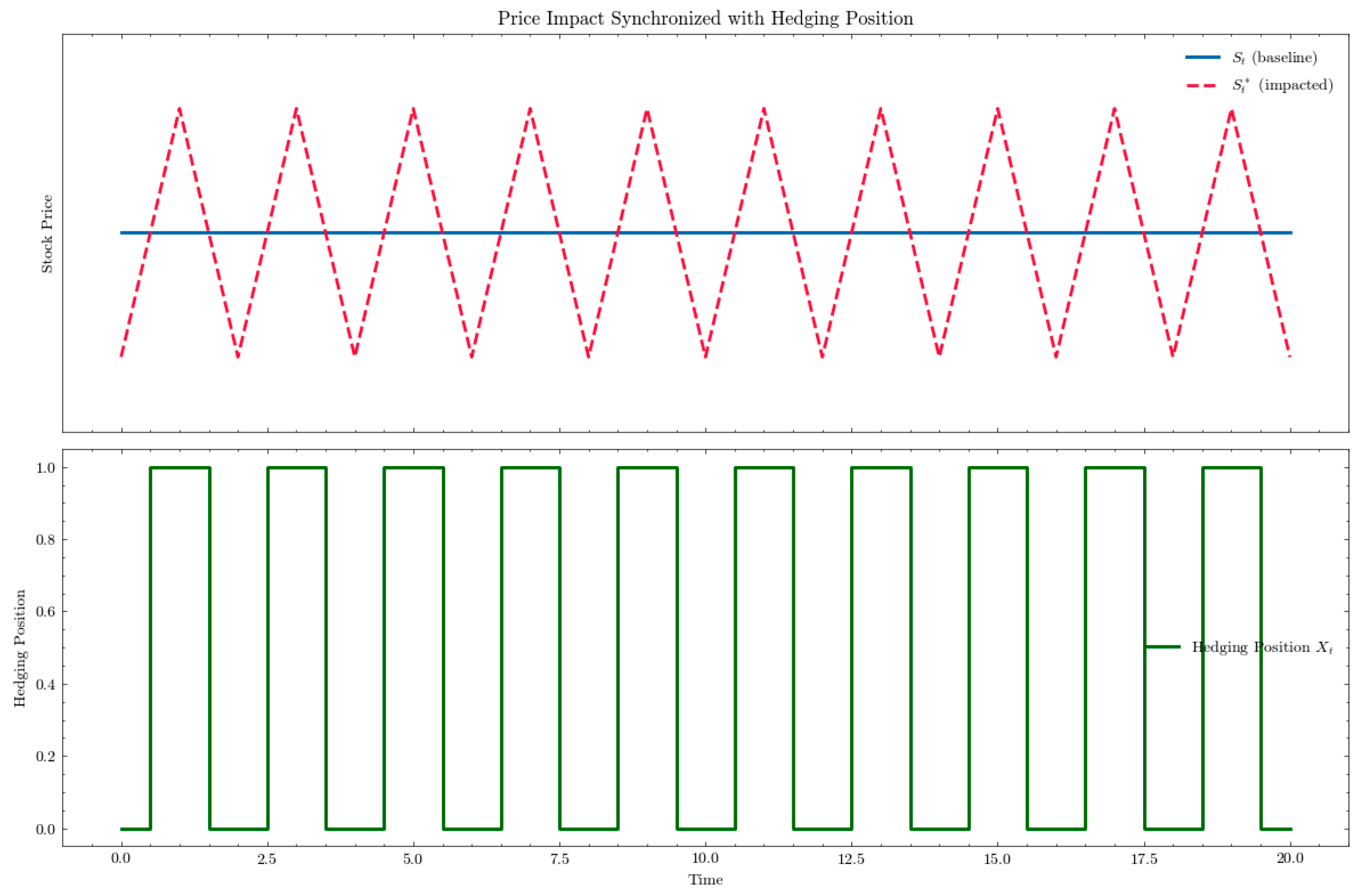This buying pressure can inadvertently create a feedback loop that increases the option’s value over time, especially in inefficient markets (Gatheral, 2010; Rogers & Singh, 2010). As the stock price rises, the call option’s delta increases, requiring the trader to buy additional shares to maintain a delta-neutral position. This buying pressure can introduce market impact, pushing the stock price even higher and further increasing the call option’s value, especially in illiquid environments (Figure 1). This cyclical behavior, driven by the interaction between market frictions and hedging adjustments, can lead to repeated oscillations in both underlying and derivative asset prices, further increasing costs to attain a delta neutral position (Anderegg et al., 2022). Such dynamics underscore the limitations of traditional hedging strategies, where the cumulative effects of slippage and permanent impact can significantly increase both hedging costs and risk exposure.

Reinforcement learning (RL) has emerged as a powerful tool for decision-making in complex, stochastic environments, offering significant advantages over rules-based or model-driven approaches (Pickard & Lawryshyn, 2023). In financial applications, RL can learn optimal strategies directly from simulated or historical market data, bypassing the need for explicit modeling of market dynamics. Recent advances in hedging research, such as Buehler’s Deep Hedging framework have enabled additional complexity when modelling hedging environments, demonstrating superiority over traditional models in the presence of transaction costs and stochastic volatility (Buehler et al., 2018). However, these frameworks often simplify market dynamics, neglecting critical frictions such as slippage and permanent impact. This paper extends the capabilities of RL-based hedging by integrating realistic cost models that reflect the challenges of trading in illiquid markets.

To overcome these challenges, we propose a deep reinforcement learning (RL) framework that determines hedging actions across discrete time steps in a dynamic trading environment with transaction costs, slippage, and market impact. Overall, we illustrate how incorporating stochastic temporary and permanent market impact feedback in the RL environment better reflects real trading conditions than simplified frictionless assumptions. In this framework, the “agent” is a trader who is hedged against a European Call option position, allowed to rebalance its hedged position with no underlying understanding of the impact models. Our approach considers short term, “transaction cost” like impacts, as well as lasting effects from excess trading by the agent, creating a more realistic framework where the true cost of hedging the security deviates from when hedging decisions are made. This deviation between the optimal hedging environments and those with frictions become more apparent as execution frequency and liquidity constraints increase.

We first design a hedging environment incorporating market frictions, liquidity constraints and transaction costs. The agent can make rebalancing decisions at every discrete timestep $t$ until expiry, with the caveat that each trade will impact the future price path of the underlying security. When the option expires, the seller will liquidate their underlying positions at the market price and pay the appropriate payoff for the option, $\max \left(K-S_t,0\right),$ where $K$ is the strike price and $S_t$ is the underlying security price at expiry.

We compare and train Deep Deterministic Policy Gradient (DDPG), Twin Delayed DDPG (TD3) and Soft Actor Critic (SAC) models to optimally hedge in these environments across various degrees of impact, with a reward function to minimize risk-adjusted hedging costs at expiry. We benchmark our results against the Black–Scholes model. Like existing deep hedging research, we will first benchmark our reinforcement learning models in an environment with only transaction costs, where there is ample liquidity to assume zero market impact. Then, we introduce liquidity constraints on the underlying asset along with market impact as a function of trade size.

The remainder of this paper is organized as follows: Section 2 reviews the existing literature on market impact, slippage, and reinforcement learning in financial applications. Section 3 details the methodology, including the RL framework, agents tested and market simulation environment. Section 4 presents the experimental results, and Section 5 concludes with a discussion of the findings and future research directions.

2. Literature Review

2.1. Market Impact

Financial markets exhibit market impact, meaning large trades can influence asset prices. Early market microstructure theory formalized this: for instance, Kyle’s seminal model described how an insider trader’s orders move prices, introducing the concept of price impact (Kyle, 1985). Later, Almgren and Chriss developed a quantitative execution model separating temporary (liquidity) costs and permanent price shifts, providing a framework to measure the cost of executing large orders (Chriss, 2001). These foundational models made clear that hedging a sizeable position is not frictionless—the act of hedging can move the market. In hedging contexts, ignoring market impact can underestimate the true cost and risk of trading. Black–Scholes hedging, for example, assumes trading does not affect prices, thus overlooking this impact. Subsequent studies have shown that incorporating market impact is crucial: Rogers and Singh explicitly examined the cost of illiquidity on option hedging and demonstrated that illiquid markets lead to significantly higher hedging costs and residual risk (Rogers & Singh, 2010). In summary, market impact models from the economics and optimal execution literature provide a necessary foundation for deep hedging in practice by quantifying how hedging trades themselves can alter market prices. Any realistic hedging strategy must account for these impacts to avoid excessive trading costs or price manipulation.

2.2. Options Pricing with Frictions

Under classical option pricing theory, dynamic delta-hedging perfectly replicates the option’s payoff, eliminating risk (Black & Scholes, 1973). However, real markets involve frictions such as discrete trading, bid–ask spreads, and transaction costs. Under these conditions, perfect replication is impossible and the Black–Scholes strategy may perform poorly (Edirsinghe et al., 1993). In fact, if every hedge trade incurs a cost, hedging continuously can accumulate so much cost that it underperforms even a static (unhedged) position. Pioneering work by Leland incorporated proportional transaction costs into option pricing by adjusting volatility in the Black–Scholes formula (Leland, 1985). The Leland approach acknowledged that hedges must be less frequent under costs, effectively widening the hedging intervals. Rogers and Singh reinforced these ideas by analyzing hedging in an illiquid market and quantifying how hedging errors grow with transaction cost magnitude (Rogers & Singh, 2010). They found that the optimal strategy often involves not fully hedging small risk exposures to avoid disproportionate costs. In summary, with market frictions, one must balance risk reduction against trading cost. Traditional models have been extended with heuristics (e.g., volatility adjustments) or utility-based pricing to handle these frictions, but such approaches can become complex and model-specific (Windcliff et al., 2006). Li and Almgren further extended his work on optimal order execution with options pricing as well, presenting modelling methods for closed form solutions for hedging options with market impact (Almgren & Li, 2016).

2.3. Machine Learning and Hedging

Given the limitations of analytic approaches in frictional markets, researchers have turned to machine learning (ML)—and particularly reinforcement learning (RL)—to derive data-driven hedging strategies. RL is well-suited to hedging because hedging is a sequential decision process under uncertainty, the type of problem RL agents were designed for (Shakya et al., 2023). An early example of bridging ML with option pricing is Halperin’s “QLBS” model, which showed that Q-learning can reproduce the Black–Scholes hedge in a simplified setting (Halperin, 2020). Building on this idea, Buehler introduced the term “Deep Hedging” for using deep neural networks to hedge options under realistic market conditions (Buehler et al., 2018). They demonstrated that a network trained via dynamic programming could learn nearly optimal hedging strategies even when assumptions like continuous trading and zero costs are relaxed. Around the same time, other studies applied modern RL algorithms to hedging. For instance, Kolm and Ritter used reinforcement learning to dynamically replicate and hedge options (Kolm & Ritter, 2019).These initial works focused on hedging a single option with its underlying, targeting delta-neutral strategies (Pickard & Lawryshyn, 2023). They confirmed that RL agents can, in simulation, approximate or improve upon the classic delta-hedging approach.

Since 2019, there has been a surge of research on deep hedging, with many variations of the hedging problem being tackled with RL. For example, Daluiso et al. incorporated risk-aversion into the RL objective, allowing the hedger’s risk preferences to influence the learned strategy (Daluiso et al., 2023). Pham et al. explored a multi-agent RL approach for hedging a portfolio of options, illustrating how multiple agents (or a single agent with a multi-dimensional action) can coordinate to hedge complex exposures (Pham et al., 2021). Xu and Dai specifically addressed delta–gamma hedging with transaction costs using RL, blending the idea of maintaining not just a delta-neutral position but also managing higher-order risks in a cost-efficient way (Xu & Dai, 2022). Another noteworthy advancement is in distributional RL: Cao et al. employed a distributional RL algorithm (a variant of Deep Deterministic Policy Gradient) to hedge not only delta but also gamma and vega risks (J. Cao et al., 2023). By allowing the RL agent to trade both the underlying and options, they showed that the agent could learn to control higher-order Greeks, with the optimal policy shifting as transaction costs or option maturities change. This indicates the flexibility of deep RL to handle multi-faceted hedging objectives under frictions.

A consistent finding across these studies is that RL-based hedging can outperform naive Black–Scholes delta-hedging in settings with frictions. For instance, Mikkilä and Kanniainen trained a deep hedging agent on empirical market data and found it consistently outperforms the Black–Scholes strategy in terms of lower hedging cost and risk, under both constant and stochastic volatility conditions (Mikkilä & Kanniainen, 2022). Notably, they report that a standard deep RL algorithm (Deep Deterministic Policy Gradient, DDPG) was unstable in training, but an improved variant was successful. This highlights the importance of algorithm selection in deep hedging. Neagu et al. presented a performance comparison of eight DRL algorithms applied to the deep hedging, including Deep Q-Learning (DQL), Proximal Policy Optimization (PPO) and Monte Carlo Policy Gradients (MCPG), while constraining the algorithms to an allocated computational budget (Neagu et al., 2025). Their findings illustrated that the policy gradient algorithms performed best relative to the Black–Scholes baseline.

DDPG was one of the first RL methods enabling continuous action spaces, ideal for adjusting a continuous hedge ratio (Lillicrap et al., 2016). However, DDPG is known to suffer from issues like reward instability and overestimation bias in value estimates, which can lead to divergence in training. To address this, Fujimoto introduced Twin-Delayed DDPG (TD3), which uses twin critics (double Q-learning) and policy delay to stabilize learning. Empirical deep hedging research reflects this improvement: the RL agent in Mikkilä & Kanniainen’s study employs a TD3-style algorithm and successfully learns a stable hedging policy, whereas the naive DDPG tended to diverge (Fujimoto et al., 2018). The twin-critic approach in TD3 effectively mitigates the overestimation issues by taking the minimum of two critic estimates, yielding more reliable value targets.

Another algorithm is Soft Actor-Critic (SAC). SAC is an off-policy actor–critic method that maximizes a stochastic policy’s rewards plus an entropy bonus, encouraging exploration and robustness (Haarnoja et al., 2018). While SAC has not yet been extensively reported in the option hedging literature, it has shown state-of-the-art performance in other financial decision-making tasks. For example, Liu implemented a SAC-based agent for a portfolio management task and achieved significantly better risk-adjusted returns than benchmarks in volatile markets (Liu et al., 2024). The success of SAC in managing a diverse asset portfolio with transaction costs suggests it is a promising candidate for option hedging under market frictions as well. In general, actor–critic algorithms like SAC and TD3 are appealing for deep hedging because they can handle continuous hedge adjustments and learn sophisticated policies from simulation or market data.

Overall, there has been limited research exploring deep hedging and market impact. Neagu et al. presented novel research for the intersection of deep hedging with market impact introducing a training framework for agentic hedging with market impact persistence. The learned policies from feed-forward neural network-based agents demonstrated success on simulated data against both Leland and Black–Scholes delta-hedging (Neagu et al., 2024). Shi et al. introduced a deep hedging for market makers under market frictions, which addresses the need of market makers to rebalance hedged positions (Shi et al., 2024). The model shows that rather than using PDEs, reinforcement learning algorithms can be successfully adapted to address the market makers’ needs for trading with realistic market frictions and risk aversions. Although out of scope for our daily trading scenario, Cheridito and Weiss introduced a multi-agent for optimal trade execution in an intraday scenario, formulating the trade execution problem as a reinforcement learning task to place market and limit orders against both naïve participants and other agents (Cheridito & Weiss, 2025). Similarly, Cao et al. presented a framework for optimizing high frequency trading strategies evaluated on NASDQAQ tick-data for liquid securities, showing that intraday approaches for DRL strategies can be applied to optimize order placement and decision making (G. Cao et al., 2024).

In summary, deep hedging research has evolved to combine financial theory with modern reinforcement learning. Key classical works—Black–Scholes for frictionless hedging, and market impact/cost models for frictional trading—provide the problem setting where perfect replication is unattainable, but optimization is possible. Machine learning approaches have filled this gap by learning dynamic hedging policies rather than relying on static pricing models, however research in environments with frictions is still limited. A variety of RL algorithms have been applied, from value-based methods to policy gradient and actor–critic methods. However, comparative evaluations remain limited in scope as well: most prior studies tested one or two algorithms in isolation, making it hard to identify the best approach across different environments. Furthermore, there has been limited exploration of deep hedging with market impact, but recent works have begun to explore DRL’s applications to both optimal order execution and hedging across simulated impact. Our work seeks to close this gap, addressing an application of deep hedging under realistic market conditions, while also illustrating a comparison of deep reinforcement learning methods and assessing their respective efficacies.

3. Methodology

In this section, we introduce our (1) market friction modelling, including temporary and permanent market impact, (2) our reinforcement learning (RL) framework, models and hyperparameters and (3) synthetic data generation. This methodology integrates a RL agent into a synthetic market environment, where slippage and permanent market impact are explicitly modeled as dynamic cost factors. The current framework does not consider limit order book dynamics, but relies on empirical assumptions from prior works on market impact, specifically the square root law. The RL agent is trained to optimize hedging strategies by minimizing total hedging costs while balancing the immediate and residual effects of its trades on the underlying asset’s price path.

3.1. Market Impact Model

We use the square root approximation for market impact to estimate the total impact estimate with daily trading frequency as a function of the liquidity traded. Bucci et al. (2019) demonstrated that the square root law, which is a function of the total trade size (in shares) as a percentage of average volume traded, provides a robust empirical approximation for market impact, effectively capturing the sublinear relationship between trade size and price deviation. This approach has been validated across various trading datasets and is commonly used in discrete-time market simulations. Where the current holdings at any time t are defined as $X_t$, and the trades at time t (which are equivalent to our agents’ actions) are defined as $A_t=\Delta X_t,$ we assume that the market impact M($A_t$) at each time step for a change in position size $\Delta X_t$ is stochastic but strictly in the direction of each trade (i.e., if $\Delta X_t$ is positive, the impact is positive as well).

Under these assumptions, the total market impact cost of size for a trade of size at execution time $t$, $A_t$, relative to the security’s average daily trading volume (ADV) of V can be modelled as:

$$M\left(A_t\right)=sign\left(A_t\right)\left|Y\right|\beta \sqrt{{\displaystyle \frac{\left|A_t\right|}{V}}}, Y~clip(N(0,1),-1,1)$$

(1)

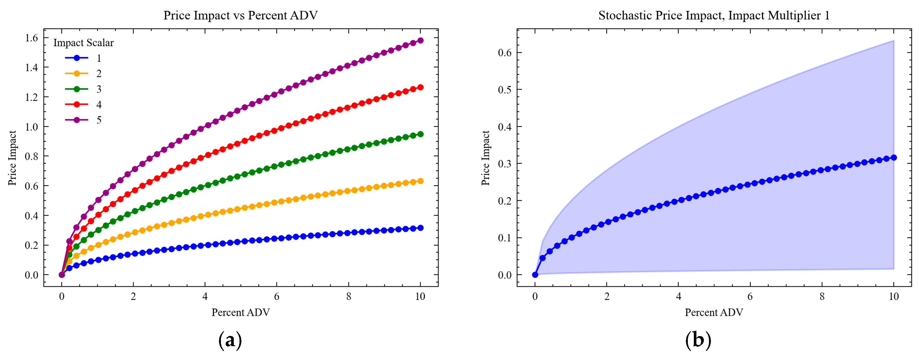
where $\beta$ is a constant impact scalar that controls the magnitude of the impact, $Y$ is a normally distributed stochastic scalar, and $sign\left(A_t\right)$ is incorporated to ensure the impact is in the same direction as the trade (Figure 2b). We incorporate a clipped stochastic variable $Y$ to better simulate the effects of market impact, given that real life trading impact can vary based on other factors including market participants, news and latent variables not modelled by our environment. Without loss of generality, we will assume that $A$ is a scaled trade size and the average daily volume $V$ is 10 times the number of shares in the options contract (i.e., $ADV=1000$ if we are hedging 1 contract with 100 shares). Figure 2a illustrates the impact distributions as a function of the trade size relative to average daily volume, specifically scaling effects on the impact magnitude as our impact scalar $\beta$ increases. Figure 2b illustrates the impact of the stochastic impact scalar $Y$, specifically the additional stochasticity that is introduced and its amplified impact as the trade size increases.

As demonstrated by (Chriss, 2001; Gatheral, 2010), the total market impact can be illustrated by two separate components: temporary impact costs $F\left(A_t\right)$ and permanent market impact $G\left(A_t\right)$. We assume that there is a reversion constant $\alpha$ which controls the percentage of impact that is temporary and permanent, i.e., what amount will be persistent in the security price following the execution of the trade. When we have both temporary and permanent market impact, we will assume that this reversion constant $\alpha$ is 50%, meaning that immediately following a trade at time $t$ the price of the underlying security is:

$$S_t^{\prime }=S_t+\alpha \cdot M\left(A_t\right).$$

(2)

where $S_t^{\prime }$ is the price path following impact and $\alpha =0.5$ is our impact reversion constant. The impact reversion constant controls the amount of impact that is realized during trade execution (temporary) at time $t$ and the residual impact that persists at $t+\Delta t$ following the trade $A_t$ (permanent). We can further deconstruct our total impact cost into a using $\alpha$,

$$F\left(A_t\right)=\alpha \cdot M\left(A_t\right);G\left(A_t\right)=\left(1-\alpha \right)\cdot \mathrm{M}\left(A_t\right).$$

(3)

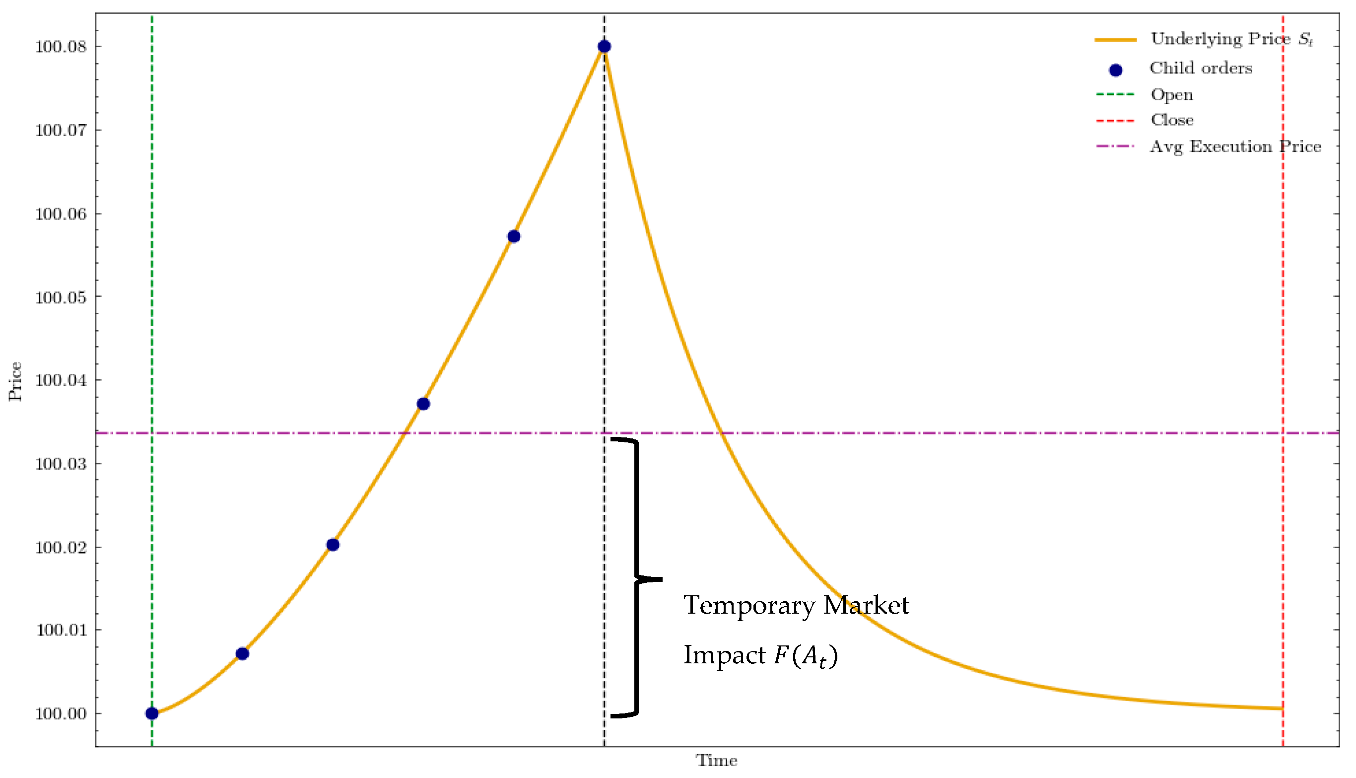
In a state of only temporary impact ($\alpha =1)$, the price of the underlying will immediately revert to the original price path following execution (Figure 3). The temporary impact component is treated as an additional execution cost, like commissions and fees. This assumption follows standard models in market impact literature who outlined temporary impacts as short-term deviations due to liquidity effects (Bucci et al., 2019).

At any time $t,$ the agent can choose to execute a trade $A_t$, resulting in an execution price of $S_t+F\left(A_t\right)$. The final transaction cost realized at time $t$, $H\left(A_t\right)$, is the sum of the total temporary impact $F\left(A_t\right)$ and transaction cost per share of c:

$$H\left(A_t\right)=A_t\cdot \left[F\left(A_t\right)+c\right].$$

(4)

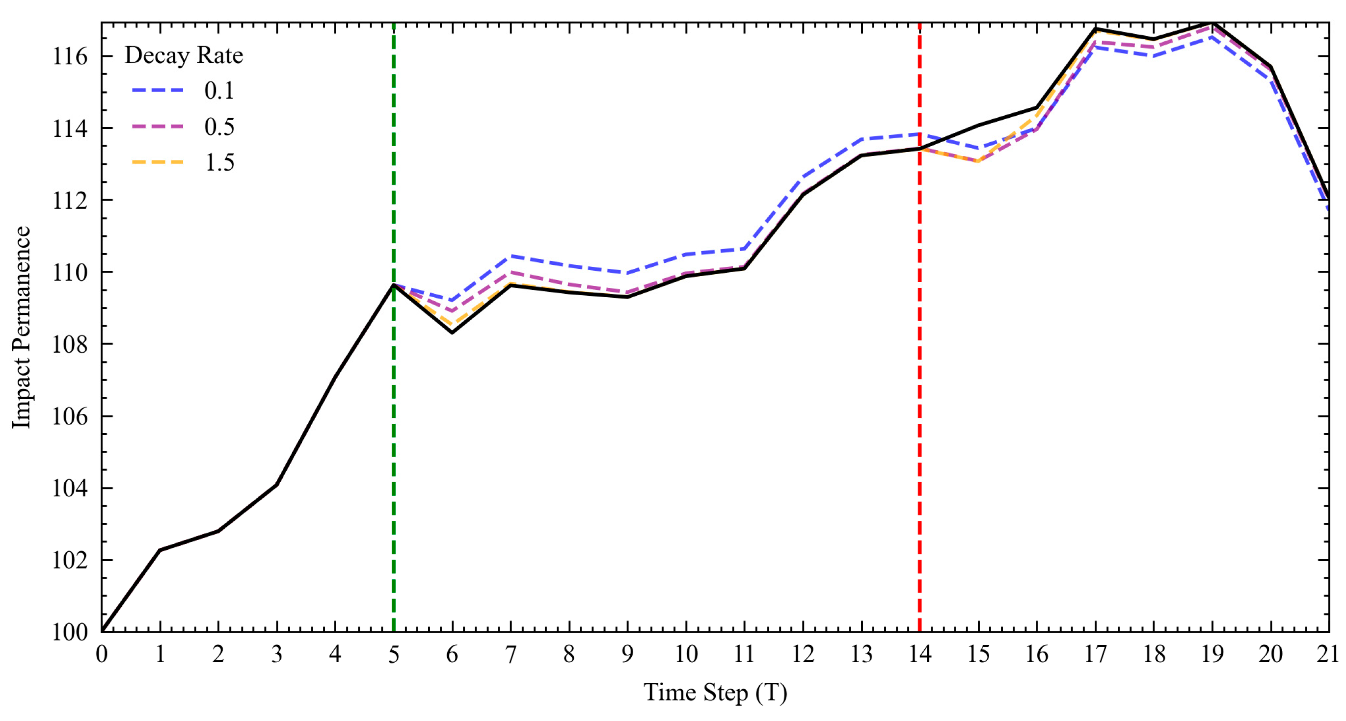
In the permanent-impact-only experiment ($\alpha =0)$, the permanent impact (Figure 4) of a trade $A_{t^{*}}$ will alter the future price path $S_t^{\prime }$ from the residual effects of the market impact. An exponential decay function of the form $e^{-\gamma \left(t-t^{*}\right)}$ inspired by (Gatheral, 2010) and (Rogers & Singh, 2010) is applied to model the gradual reversion of the initial impact $G\left(A_{t^{*}}\right)=(1-\alpha )M\left(A_{t^{*}}\right)$ at time $t^{*}$ over time with a decay rate of $\gamma$. The impact at time $i$ from a trade at $j$ (where $i>j$) can be expressed as $G\left(A_j\right)e^{-\gamma (i-j)}$. The total accumulated impact $J\left(\mathit{A}\right)$ at time $t$, where $\mathit{A}$ is a vector of all trades occurring before $t,$ is therefore:

$$J\left(\mathit{A}\right)=\sum _0^{t-1}G\left(A_i\right)\cdot e^{-\gamma \left(i-t^{*}\right)},$$

(5)

resulting in a future price path $S_t^{*}=S_t+J\left(\mathit{A}\right)$.

To note is that the proposed market impact model does not factor in order book dynamics, as we assume that hedging decisions are daily metaorders with a total impact rather than smaller intraday orders. Further studies could further integrate order book simulations, which can serve as additional inputs for an intraday hedging agent.

3.2. Reinforcement Learning Framework

Our environment reflects a discrete-time trading world across continuous action spaces, with daily trading across $t$ and a continuous action space. In this environment, the trader (agent) is short one unit of an at the money European call option, with $S_o$ = $K$, $T$ days to maturity and an annual lognormal price volatility of $\sigma .$ At every timestep, the trader is given the option to reoptimize their position until the option expires. The agent’s primary goal is to minimize the cumulative cost of hedging one short call option position across various degrees of market impact and transaction costs.

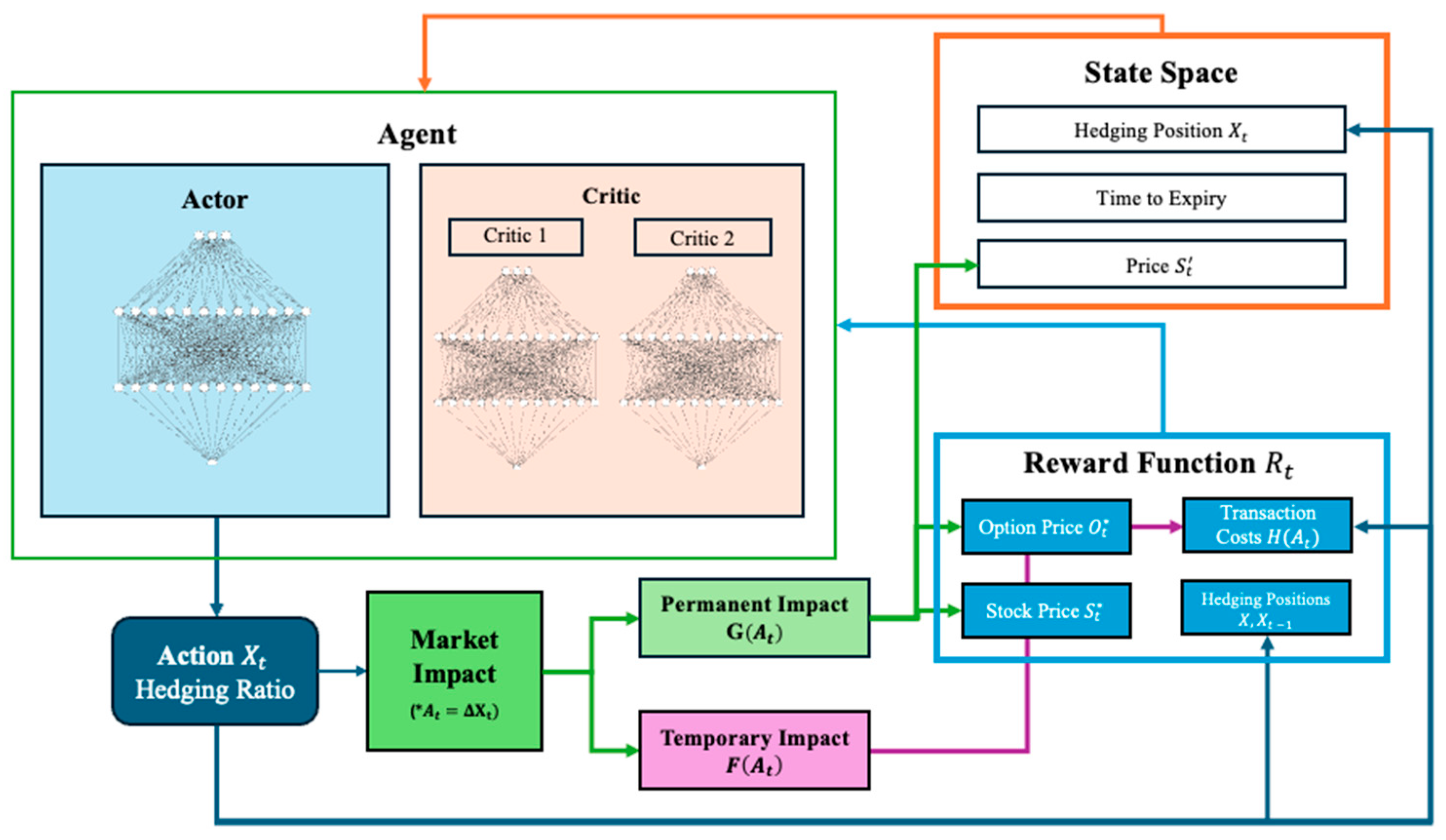
We integrate the market impact models into a discrete-time reinforcement learning environment for delta hedging, where the agent hedges a short position on a European call option. The agent (Figure 5) takes actions $X_t$ (same as the hedging position size in Section 3.1) to rebalance its hedging position at a daily frequency. $X_t$ represents a ratio of the total number of hedged securities owned by the agent, bound between zero and one, meaning that the agent cannot short the underlying security. A hedge position of one is equivalent to owning 100 underlying shares of the option in the environment assuming we are hedging 1 options contract. Each trading decision at time $t$ results in both a fixed cost (broker and exchange fees) and subsequent market impact at $t+1$.

The agent’s observation space ${\mathcal{S}}_t$ consists of:

• Underlying security price $S_t$ ($S_t^{*}$ if permanent market impact is enabled): If there is permanent market impact, the agent only sees the price following the cumulative residual impacts $J\left(\mathit{A}\right)$, and cannot see the original underlying price path $S_t$
• Current hedging position $X_t$: This represents how hedged the agent currently is.
• Time to expiry $T-t$: This illustrates the amount of time the agent has until the option payout occurs, or the time left in the training episode.

The agent itself has no knowledge of option Greeks, and utilizes only market information to decide its next hedging position $X_t$.

3.2.1. Reward Function

The deep hedging problem can also be framed as a PnL maximizing utility function in the form of a mean-variance optimization problem, treating our holdings as a portfolio at each timestep $t$ with a risk aversion parameter $\lambda$ to penalize high PnL variance, given by

$$\mathrm{m}\mathrm{a}\mathrm{x}(\mathbb{E}\left[Z_T\right]-\lambda \mathbb{V}\left[\left(Z_T\right)\right])$$

(6)

where portfolio wealth $Z_T$ is the sum of wealth increments $\Delta Z_t$

$$Z_T=Z_o+\sum _{t=1}^T\Delta Z_t$$

(7)

Resulting in $E\left[Z_t\right]=Z_o+{\Sigma }_t\mathbb{E}\left[\Delta {\mathrm{Z}}_{\mathrm{t}}\right].$ Similarly to Kolm and Ritter’s derivation, we that the wealth increments are uncorrelated for $s\ne t,\mathrm{i}.\mathrm{e}.,cov\left(\Delta Z_t,\Delta Z_s\right)=0$ (Kolm & Ritter, 2019).

We restructure the optimization function to a more simplified objective for our hedging agent,

$$\mathrm{m}\mathrm{i}\mathrm{n}\sum _{t=0}^T(\mathbb{E}\left[-\Delta Z_t\right]+\lambda \mathbb{V}\left[(\Delta Z_t)\right])$$

(8)

where $\Delta Z_t$ is the change in portfolio value between each discrete time step and $T$ is the total days until expiry when the option is first sold. The original implementation of Equation (8) by Almgren and Chriss was presented to optimize for a trading execution strategy that minimized total losses. As shown in the derivation by (Kolm & Ritter, 2019), this can be simplified into a reward function, $R_t$, by observing the changes in $Z_t$ after each rebalance period,

$$R_t:=E\left[\Delta Z_t\right]-\lambda E\left[\Delta Z_t^2)\right]$$

(9)

recasting the objective function $\mathbb{E}\left[Z_T\right]-\lambda \mathbb{V}\left[\left(Z_T^2\right)\right]$ into a reward after each action in our reinforcement learning setting.

The PnL (profit and loss) $Z_t$ will have 3 components: the value of the options position, $O_t$ value of the underlying security $S_t$, and total transaction costs. At expiry, the reward function reflects the cost of liquidating the hedged position and the option payoff at expiry. However, unlike other studies, with this approach, the deviations in PnL are not exclusively from transaction costs, but instead are further complicated by slippage and market impact. We will use a higher $\lambda$ parameter of 1.5 to discourage excess trading and subsequent price manipulation by the agent.

We define the total portfolio value $Z_t$ to be:

$$Z_t=X_t{S}_t+C_t-O\left(S_t,K,T,t,\sigma \right)-\sum _{s=1}^{t}H\left(A_s\right),$$

(10)

where $X_t{S}_t$ is the value of the underlying security holdings, $C_t$ is the value of the cash account, $O\left(S_t,K,T-t,\sigma \right)$ is the value of the option given a time to expiry $T-t$ and $H\left(A_s\right)$ is the transaction cost of all rebalancing trades prior to time $t$ (which includes temporary market impact). The value of the call option is calculated at each time step using the Black Scholes equation. The cash account $C_t$ tracks the value of the financing required to purchase the hedged positions; we also assume that the agent exists within a zero-interest rate environment, which applies to both positive cash (from liquidated shares) as well as negative funds resultant from borrowing. We assume that maximum borrowing capacity of the agent is limited to the number of shares required to fully hedge the options position (i.e., achieve a hedge ratio of 1).

Due to the portfolio being self-financing, the wealth increment at time $t$ from the holdings at time $t-\Delta t,\Delta Z_t$ can be expressed as:

$$\Delta Z_t=X_t\left(\Delta S_{t+\Delta t}\right)+\Delta C_t-\left[O\left(S_{t+1},K,T-t\right)+O\left(S_t,K,T-t-\Delta t\right)\right]-H\left(A_t\right),$$

(11)

where $X_t\left(\Delta S_{t+\Delta t}\right)$ is the change in security value of the underlying position. In practice $C_t$ reflects the cash needed to finance our hedge. However, as we assume an interest-free environment and that cash flows are used only to adjust the hedged position, the cash account $C_t$ behaves as a passive balancing term rather than an active wealth component.

Permanent market adds an additional layer of complexity to both the value of the underlying and the derivative. In this scenario, the subsequent price paths are redefined following each action ${\Delta X}_t,$ with $S_t^{\prime }$ and $O_t^{\prime }$ representing the new underlying and option price paths, respectively. Each are recalculated after finding the cumulative residual impact $J\left(\Delta \mathit{X}\right).$ The price impact of the trade will be immediately reflected in $\Delta S_t$ and $\Delta O_t$ in the reward calculation. The PnL under both slippage and price impact can then be expressed as:

$$\Delta Z_t=X_t\left[\Delta S_t^{\prime }\right]-\left[O\left(S_t^{\prime },K,T-t+\Delta t\right)+O\left(S_t,K,T-t\right)\right]-H\left({\mathrm{A}}_t\right).$$

(12)

3.2.2. Model Parameters

We compare three different continuous off-policy deep reinforcement learning algorithms:

• Deep Deterministic Policy Gradients (DDPG);
• Twin Delayed DDPG (TD3);
• Stochastic Actor-Critic (SAC).

DDPG introduces a deterministic actor and critic pair to learn a continuous hedge ratio from replay-buffer data, but its single-critic design and heuristic noise exploration can suffer from value over-estimation and unstable convergence in volatile markets. TD3 tackles these weaknesses with three tweaks: (i) twin critics and a “min” target to damp over-optimism, (ii) delayed policy updates so the actor trains on more reliable Q-values, and (iii) target-policy smoothing that averages Q-targets over a noisy action neighborhood. SAC goes a step further by learning a stochastic, entropy-regularized policy. Maximizing expected return plus an entropy bonus keeps the agent exploring a spectrum of hedge sizes rather than locking into one deterministic action, a property that helps it navigate the multi-modal, noisy reward landscape created by liquidity shocks. Like TD3, SAC uses twin critics to curb over-estimation (J. Cao et al., 2020, 2023; G. Cao et al., 2024) but its entropy term automatically tempers policy shifts and improves sample efficiency.

Empirical studies show SAC and TD3 generally outperform vanilla DDPG on continuous-control and trading tasks, with SAC excelling when market dynamics are highly stochastic or non-stationary. Together, these algorithms form a progression of increasing robustness for deep hedging: DDPG for baseline continuous control, TD3 for bias-corrected stability, and SAC for entropy-driven adaptability in the face of transaction costs and market impact.

We train the agents using the StableBaselines 3 implementation of each algorithm. We choose to use similar hyperparameters in performance evaluations across all three models. The parameters were originally calibrated on a no-friction hedging environment using DDPG, equalized to (1) maximize training efficiency, (2) provide a comparable benchmark between the three algorithms, and (3) prevent overfitting across different market conditions.

The hyperparameters for our simulation environment are:

• Policy Updates: we update the policy at every 4 timesteps. This frequency was chosen to find a balance between update frequency and training time; we found that more frequent updates did not drastically improve learning speed but did significantly increase training time per agent. Our update frequency corresponds to a policy update 5 times per episode;
• Replay Buffer Size: A buffer of size 100,000, enabling the agent to learn from a diverse set of past experiences, improving sample efficiency and avoiding overfitting to recent market conditions. Buffer sizes of ${10}^3,{10}^4,{10}^5,{10}^6,$ and 10⁷ were tested;
• Soft Update Parameter (τ): A target network soft update coefficient of 0.0001, which ensures stable convergence by gradually updating the target network weights to prevent sudden shifts in learning;
• Optimizer: The Adam optimizer is employed, with relatively low learning rates of ${10}^{-4}$ for the actor and critic networks. This implementation is the same as presented in (Mikkilä & Kanniainen, 2022);

The hyperparameters were chosen after running no-transaction cost simulations of the DDPG algorithm, prioritizing time to convergence as well as total training time, unless otherwise stated. For the neural network hyper-parameters, we use the default implementation with two fully connected layers for both the actor and critic networks, each with 256 units. Furthermore, we choose to apply ReLU activation functions within our fully connected networks, consistent with the approach by (J. Cao et al., 2020).

3.2.3. Data

We use Geometric Brownian Motion (GBM) to simulate the underlying price path without market impact until expiry. The GBM model assumes that the price path $S_t$ following the stochastic differential equation:

$$d{S}_t=\mu S_{t}dt+\sigma S_t{W}_t.$$

(13)

We assume that the agent rebalances its hedging position discretely rather than continuously. In this setting, the GBM model is discretized as:

$$S_t=S_0\exp \left(\left(\mu -{\displaystyle \frac{{\sigma }^2}{2}}\right)t+\sigma Z\sqrt{t}\right)$$

(14)

where $\mu$ is the stock’s annualized expected return and $\sigma$ is the annualized volatility, and $Z_t~N(0,1)$ is a random normal variable and $t$ is a discrete time step, specifically 1 day. We set $\sigma =0.2$, $S_0=100$ and $\mu =0.05$ with a time to expiry of 1 month, corresponding (21 trading days). We generate 20,000 independent price paths, which are reused across different training environments.

We price the environment’s option using the Black–Scholes model, which provides a closed form solution for pricing our European call option. In frictionless environments, the Black Scholes model provides a perfect hedge and risk neutralization.

The Black–Scholes model for pricing call options is used as a benchmark to calculate the European call option price and its respective delta across $t$, where the call option price $C(S_t,K,T-t,r,\sigma )$ is:

$$C\left(S_t,K,T,t,r,\sigma \right)=S_t\Phi \left(d_1\right)-K{e}^{-r\left(T-t\right)}\Phi \left(d_2\right)$$

(15)

where $d_1=(\ln \left({\displaystyle \frac{S}{K}}\right)+{\displaystyle \frac{r+{\sigma }^2}{2}}(T-t))/\sigma \surd T$ and $d_2=d_1-\sigma \sqrt{T}.$ $T$ is the time to expiry at the start of the episode, $K$ is the strike price, $r$ is the risk free interest rate and $\sigma$ is the underlying volatility, $\Phi$ denotes the cumulative distribution function of the standard normal distribution. The delta, $\Delta$, used in a standard Black Scholes hedge is

$$\Delta =\Phi \left(d_1\right).$$

(16)

3.2.4. Volatility Estimation Under Permanent Market Impact

To account for fluctuations in price when permanent market impact $G\left(A_t\right)$ is present, we introduce an adaptive volatility model to price the options rather than using a constant volatility of $\sigma =0.2$. This new measure ${\sigma }_t^{\mathrm{*}}$ does not affect the future price path $S_t$, but instead is an episode-specific volatility estimate that is meant to reflect the implied volatility of the price path $S_t^{\mathrm{*}}$.

We employ a $IGARCH\left(\mathrm{1,1}\right)$ model that updates volatility estimates in response to the agent’s trading activity. In the $IGARCH\left(\mathrm{1,1}\right)$ formulation, the variance at timestep $t,{\sigma }_t^{\mathrm{*}},t^{\mathrm{*}}>t$ is determined by a constant term $\omega$, the most recent squared return ${ϵ}_t^2$ and the previous variance ${\sigma }_t^2$. Mathematically, the model is expressed as ${\sigma }_{t^{*}}^2=\omega +{ϵ}_t^2+{\sigma }_t^2$. Here, ${\mathsf{ϵ}}_t$ represents the shock term at time t, or in our case the last observed return of the underlying security $S_t$ over the latest interval that includes the permanent market impact.

Prior to agent intervention $(t<0),$ we simulate a rolling window of daily returns based on a standard geometric Brownian motion with $\sigma =0.2$. This forms the basis for initializing ${\sigma }_0^{\mathrm{*}}.$ Once the agent begins trading ($t\ge 0)$, the returns ${ϵ}_t$ are recalculated at each timestep using the updated $S_t^{\mathrm{*}}$ and the $IGARCH\left(\mathrm{1,1}\right)$ process continues to update ${\sigma }_t^{\mathrm{*}}$ accordingly. By aligning the derivative’s volatility and returns influenced by $S_t$, any strategic distortion of $S_t^{\mathrm{*}}$ by the agent—particularly under permanent impact—is captured in option pricing and reflected in the reward structure.

Following each action $A_t$, the environment recalculates the volatility of the underlying of $S_t^{\mathrm{*}}$ to include the underlying returns ${ϵ}_t={\displaystyle \frac{S_t^{\mathrm{*}}-S_{t-1}^{\mathrm{*}}}{S_{t-1}^{\mathrm{*}}}}$. Large or aggressive trades result in more significant price moves ${ϵ}_t$, which subsequently inflate ${\sigma }_t^{\mathrm{*}}$ via the $IGARCH$ update. Because this volatility is then used to value the option (e.g., via Black–Scholes or numerical methods), higher ${\sigma }_t^{\mathrm{*}}$ increases the cost of hedging and penalizes the behavior in the reward function. The volatility adjustment is intended to increase the price of the option if the agent trades aggressively (Figure 6), consequently increasing the cost of the option and decreasing rewards.

4. Results

4.1. Comparison of DDPG, TD3 and SAC

In this section, we show the numerical results of comparing in-sample and out-of-sample training performance for 3 continuous, off-policy models: DDPG, TD3, and SAC. We analyze each models’ ability to maximize the total objective $\Sigma R_t$ and converge throughout the 20,000 episodes.

First, we train all 3 models in our simplest experimental setup, the transaction cost-only environment with a transaction cost of 5 cents per share.

Table 1. Model Comparison, Transaction Cost Only. $c=0.05.$ (Best results are outlined in bold).

Metric	Delta	DDPG	TD3	SAC
P&L $\mathbb{E}(\Sigma \Delta Z_t)$	−11.18	−7.97	1.42	7.66
P&L Std $\sigma (\Sigma \Delta Z_t)$	118.14	83.60	89.15	70.58
Rewards $\mathbb{E}(\Sigma R_t)$	−2.19	−1.04	−0.86	−0.61
Rewards Std $\sigma (\Sigma R_t)$	2.90	1.45	1.20	1.13
CVaR * 0.05	−211.89	−158.78	−144.57	−122.99
Transaction Costs	10.98	9.20	8.11	9.02
Training Time (seconds, 20,000 Episodes)	-	255	227	348

Row-wise bolded metrics highlight the best performance across each metric. * CVaR is calculated using the total Profit and Loss ($\mathbb{E}(\Sigma \Delta Z_t))$.

compares the model outcomes when trained in a transaction cost only environment, providing a benchmark for RL agent performance in more complex market scenarios. In Figure 7, we see that the DDPG and TD3 and algorithms illustrate very similar learning patterns, with relatively quick convergence and stable out-of-sample performance, with both achieving convergence at approximately $\mathbb{E}\left[R_t\right]\approx -2$. On the other hand, SAC continues to illustrate continued learning past 20,000 episodes, with its out-of-sample reward continuing to increase in an almost linear fashion. SAC took much longer to train per episode, highlighting the added computational power needed for the entropy-based learning. We continued to train the SAC model in this environment until 30,000 episodes, and saw its out-of-sample reward converge to $\mathbb{E}\left[R_t\right]\approx -1.$

We then initiate a new comparison environment with both permanent and temporary market impact. In this section, we use lower magnitude parameters as well to serve as a benchmark case when lighter market frictions are introduced: we use a transaction cost $c$ of 1 cent/share, an impact multiplier $\beta$ of 1 and an impact decay rate $\gamma$ of 1. In Figure 8, we illustrate the average reward per episode achieved on both the training and testing data, where we tested the model performance every 500 episodes on the testing data. Immediately, we see that DDPG and TD3 demonstrated strong convergence on the training data, reaching similar and stable points of convergence past 2000 episodes. However, we further see that DDPG algorithm fails to generalize as well as TD3 when exposed to new price paths with the same parameters ($\mu =0.05$ and $\sigma =0.2$), with a much higher volatility between evaluation periods. TD3 on the other hand maintains a relatively similar in-sample and out-of-sample performance, with a deviation of only 0.5. Both TD3 and DDPG converge relatively quickly in-sample past episode 3000 and maintain a stable upwards learning path with little translation to its out-of-sample performance. SAC on the other hand has a large divergence between in-sample and out-of-sample performance across time, even in later stages of training. Although the SAC algorithm appears to continue learning on the training dataset, this does not translate well to its performance on the validation dataset, especially in the more complex environment.

The differences between TD3 and SAC can be better visualized in where we directly compare the relative performance (out-of-sample reward minus in-sample reward) of the two algorithms in Figure 7, Although TD3 is able to sustain relatively high-performance metrics, illustrates higher volatility in evaluation episodes, whereas the SAC agents perform better out-of-sample. This is likely due to its added exploration and stochasticity during training, whereas our evaluation process for both models rely on deterministic predictions. TD3’s in-sample metrics rarely surpassed its out-of-sample metrics with a high degree of magnitude at each evaluation point, seems to maintain a relatively stable transfer of its learned parameters when tested out-of-sample.

In

Table 2. Permanent Impact and Slippage ($\beta =1,\gamma =0.75,c=0.05)$.

Metric	Delta	DDPG	TD3	SAC
P&L $\mathbb{E}$ ($\Sigma \Delta Z_t)$	−66.52	−28.70	−25.06	−30.77
P&L Std $\sigma (\Sigma \Delta Z_t)$	130.82	94.62	89.46	72.15
Rewards $\mathbb{E}(\Sigma R_t)$	−2.91	−1.40	−1.28	−0.98
Rewards Std $\sigma (\Sigma R_t)$	3.69	1.79	1.66	1.16
CVaR 0.05	−269.00	−192.25	−182.75	−145.53
Transaction Costs	11.06	7.11	7.53	8.31
Training Time (seconds, 20,000 Episodes)	-	228	267	583

Bolded metrics denote the best performance across Delta, TD3 and SAC across each experiment.

, we see that DDPG underperforms both SAC and TD3 in the more complex environment as well, albeit slightly. TD3 and SAC can achieve lower overall variance in both PnL and total rewards, including a lower conditional value at risk. Furthermore, we see that SAC achieves an incredibly low relative standard deviation compared to both agents, especially as training continued, whereas DDPG and TD3 had limited past 10,000 episodes (Figure 8). Counter to our expectations, this is achieved while SAC trades more (~17% relative to DDPG and ~10% relative to TD3) in the environment with both sets of market impact, implying that the agent is learning to trade more than the deterministic algorithms while achieving a higher PnL.

Following our comparative analysis of SAC, TD3, and DDPG, we have chosen to focus our subsequent experiments exclusively on SAC and TD3, each for distinct reasons. TD3 demonstrates notably faster training times coupled with solid overall performance; however, it does not achieve SAC’s consistently higher average rewards and lower reward variance, even after extended training periods. Both SAC and TD3 exhibit rapid convergence within a relatively small number of training episodes, with marginal improvements beyond approximately 15,000 episodes, whereas DDPG shows a markedly slower learning rate. The following sections will provide an in-depth analysis of the hedging strategies derived by each algorithm under varying test scenarios and complexity levels, as well as specific case studies of robustness among each model’s respective policies.

4.2. Transaction Cost Only Experiments

This section serves as a baseline to evaluate the performance of reinforcement learning (RL) agents under conditions devoid of market frictions. The objective is to compare the hedging efficiency of our RL agents (TD3 and SAC) against traditional Black–Scholes delta hedging under varying transaction costs ($c)$ and to verify the results of existing literature. In the subsequent sections, we will add additional frictions to the environment to assess trading efficacy. We train independent agents in 5 different environments of varying transaction costs per share, ranging from 1 cent per share to 20 cents per share.

Table 3. Comparison of TD3 and SAC against Delta Hedging, Transaction Cost only Experiment.

$\mathit{c},$ Cost per Share ($)	$\mathbf{Profit}\mathbf{and}\mathbf{Loss}\mathbb{E}$$\left(\mathsf{\Sigma }\mathsf{\Delta }{\mathit{Z}}_{\mathit{t}}\right)$			$\mathbf{Rewards}\mathbb{E}\left(\mathsf{\Sigma }{\mathit{R}}_{\mathit{t}}\right)$			CVaR 0.05			Transaction Costs
	Delta	TD3	SAC	Delta	TD3	SAC	Delta	TD3	SAC	Delta	TD3	SAC
0.01	6.5 ± 109.6	7.2 ± 81.7	6.8 ± 63.8	−1.7 ± 3.0	−0.9 ± 1.5	−0.5 ± 1.0	−174.7	−142.2	−102.6	2.2	1.5	1.9
0.03	2.2 ± 111.2	6.8 ± 79.7	4.7 ± 62.6	−1.8 ± 2.9	−0.8 ± 1.2	−0.5 ± 1.0	−185	−121	−102	6.5	5.2	5.9
0.05	−1.2 ± 107.9	0.5 ± 75.5	−0.9 ± 61.1	−1.7 ± 2.8	−0.7 ± 1.3	−0.5 ± 0.9	−185.8	−143.1	−110.6	10.7	8.8	9.5
0.1	−14.5 ± 109.7	−6.0 ± 73.6	−9.6 ± 59.3	−1.9 ± 3.0	−0.7 ± 1.0	−0.6 ± 0.9	−204.4	−129.5	−110.3	21.6	15.8	19.3
0.2	−40.4 ± 111.3	−24.0 ± 72.9	−25.7 ± 62.6	−2.2 ± 3.1	−0.9 ± 1.1	−0.8 ± 0.9	−231.4	−151	−130.7	43.1	33.1	34.7

Bolded symbols denote the best performance for each metric.

illustrates the rewards, conditional value at risk, and total transaction costs in the episode across 5 different experiments.

The results demonstrate that our experimental setup can replicate the relative results of existing deep hedging research, with TD3 and SAC slightly the delta hedging benchmark across most metrics and environments. As expected, delta hedge exhibits lower PnL and episodic reward, in addition to a much higher standard deviation on both metrics. Both agents trade less frequently than the delta hedging agent (with transaction costs being proportional to total shares traded) and lower the standard deviation of P&L and rewards in addition to minimizing conditional value at risk. SAC surpasses TD3 in lowering volatility, with a lower reward and L volatility in addition to a lower value at risk across all environments. Counter to our original expectations, SAC achieves both a smaller total risk and high relative P&L with larger with higher turnover compared to TD3. TD3 on the other hand learns to reduce total costs by trading less frequently, consistently having the lowest transaction cost of the three.

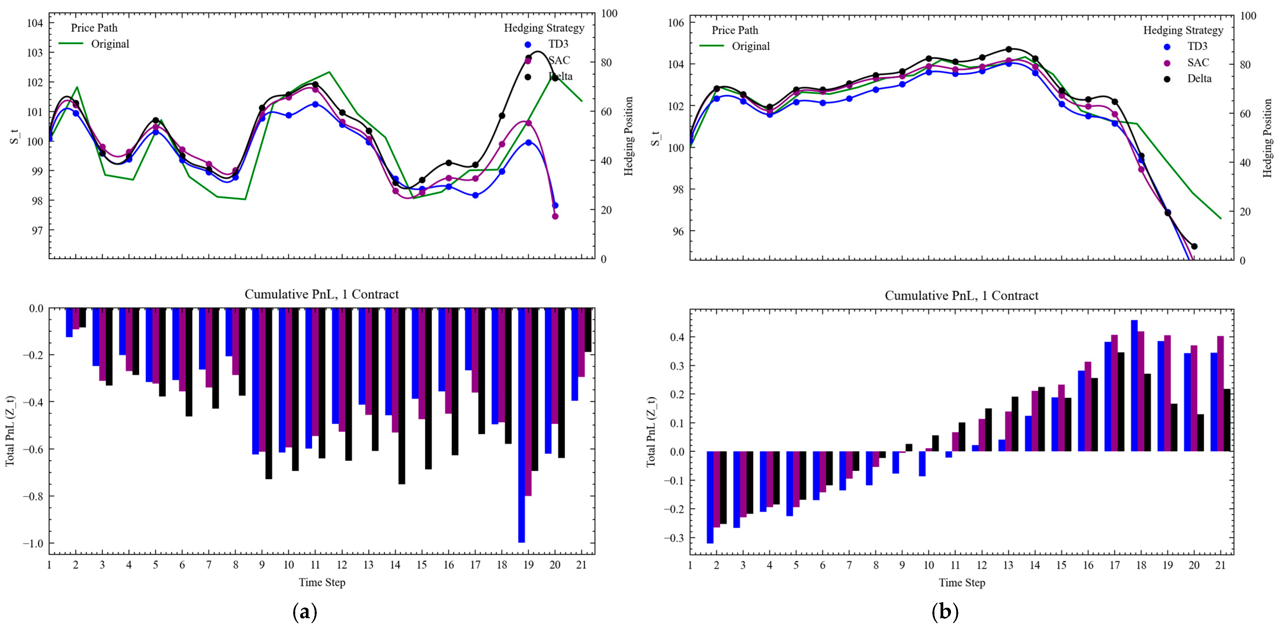
In Figure 9 we illustrate two examples of hedging patterns when the cost to trade is higher at $c=0.10.$ We see that when the option expires in-the-money (left), the agents hold onto the shares as long as possible, but begin to liquidate their hedging positions slowly once they are confident the option is going to expire in-the-money, with SAC liquidating slightly faster than TD3. Overall, the agents remain underhedged compared to the benchmark, but can earn small profits from their trades as the underlying prices move. The delta hedging strategy on the other hand holds onto the positions, resulting in a large liquidation cost at expiry. When the option expires at the money (right), we see that the agents maintain a similar trading pattern in the presence of high hedging costs, closely emulating the delta hedge until the close. SAC is more careful in its approach, maintaining a closer hedge to the delta hedge relative to TD3, which begins liquidation consistently with 3 days to expiry.

4.3. Temporary Impact Only

Across this set of results, we illustrate the RL agents’ behavior when the environment has transaction costs $c$ and temporary impact costs $F\left(A_t\right)$ following each transaction. This scenario emphasizes the agent’s ability to adapt to cost dynamics that are proportional to trade size, offering a robust test of hedging strategies under transient market frictions. In our reward function, the temporary impact is immediately reflected in the reward at time $t$. The total slippage cost, $F\left(A_t\right)$ is proportional to the magnitude of the total shares traded relative to the average daily volume (ADV). For simplicity, all environments hedge a single option contract. We set the environment ADV to 1000 shares and assume a constant trading cost $c$ of 5 cents per share.

The temporary market impact effectively introduces an additional cost (slippage) to every trade, however unlike a transaction cost, the slippage cost per share scales with the agent’s trade size due to the stochastic impact scalar Y.

Table 4. Transaction Costs and Slippage, performance across impact multiplier $\beta$ (10,000 episodes).

$\mathit{\beta }$	$\mathbf{Profit}\mathbf{and}\mathbf{Loss}\mathbb{E}$$\left(\mathsf{\Sigma }\mathsf{\Delta }{\mathit{Z}}_{\mathit{t}}\right)$			$\mathbf{Rewards}\mathbb{E}\left(\mathsf{\Sigma }{\mathit{R}}_{\mathit{t}}\right)$			CVaR 0.05			Transaction Costs
	Delta	TD3	SAC	Delta	TD3	SAC	Delta	TD3	SAC	Delta	TD3	SAC
0.1	−48.6 ± 110.1	−30.2 ± 89.4	−35.8 ± 55.7	−2.3 ± 3.0	−1.4 ± 1.8	−0.8 ± 0.8	−237	−175	−133.6	43.2	30.9	40.3
0.25	−57.9 ± 112.0	−27.6 ± 86.4	−36.1 ± 69.9	−2.5 ± 3.2	−1.2 ± 1.5	−1.0 ± 1.2	−254.3	−180.6	−161	43.3	26.8	34.6
0.5	−72.4 ± 114.2	−53.5 ± 62.1	−41.1 ± 74.6	−2.7 ± 3.4	−1.0 ± 0.9	−1.2 ± 1.3	−266.4	−161.2	−165.9	43.3	43.1	32.3
0.75	−89.3 ± 118.8	−47.7 ± 80.6	−52.7 ± 59.9	−3.0 ± 3.6	−1.3 ± 1.4	−1.0 ± 1.0	−302	−199.3	−156.4	43.7	32.2	36.4
1	−102.8 ± 120.3	−50.7 ± 91.3	−54.9 ± 81.7	−3.3 ± 3.9	−1.6 ± 1.9	−1.4 ± 1.6	−317.2	−219.7	−211.6	43.2	26.3	32.4
2	−162.6 ± 137.6	−70.5 ± 101.2	−68.9 ± 93.5	−4.9 ± 5.3	−2.1 ± 2.1	−1.8 ± 2.0	−411.1	−252.9	−243.6	43.1	26.7	27.2
3	−222.2 ± 159.9	−86.1 ± 107.4	−89.6 ± 93.7	−7.0 ± 7.3	−2.6 ± 2.1	−2.1 ± 1.9	−510.7	−270.4	−265.6	43.4	24.7	27
4	−285.8 ± 186.5	−95.5 ± 120.6	−89.9 ± 117.8	−9.9 ± 10.5	−2.7 ± 2.8	−2.6 ± 2.6	−625.3	−320	−316.6	43.4	23	23.9
5	−343.4 ± 217.1	−108.4 ± 127.5	−104.7 ± 124.7	−13.3 ± 14.3	−2.9 ± 2.8	−2.8 ± 2.9	−732.8	−352.4	−348.8	43.1	24.8	24.3

Bolded metrics denote the best performance across Delta, TD3 and SAC across each experiment.

illustrates the results across various levels of impact magnitude. 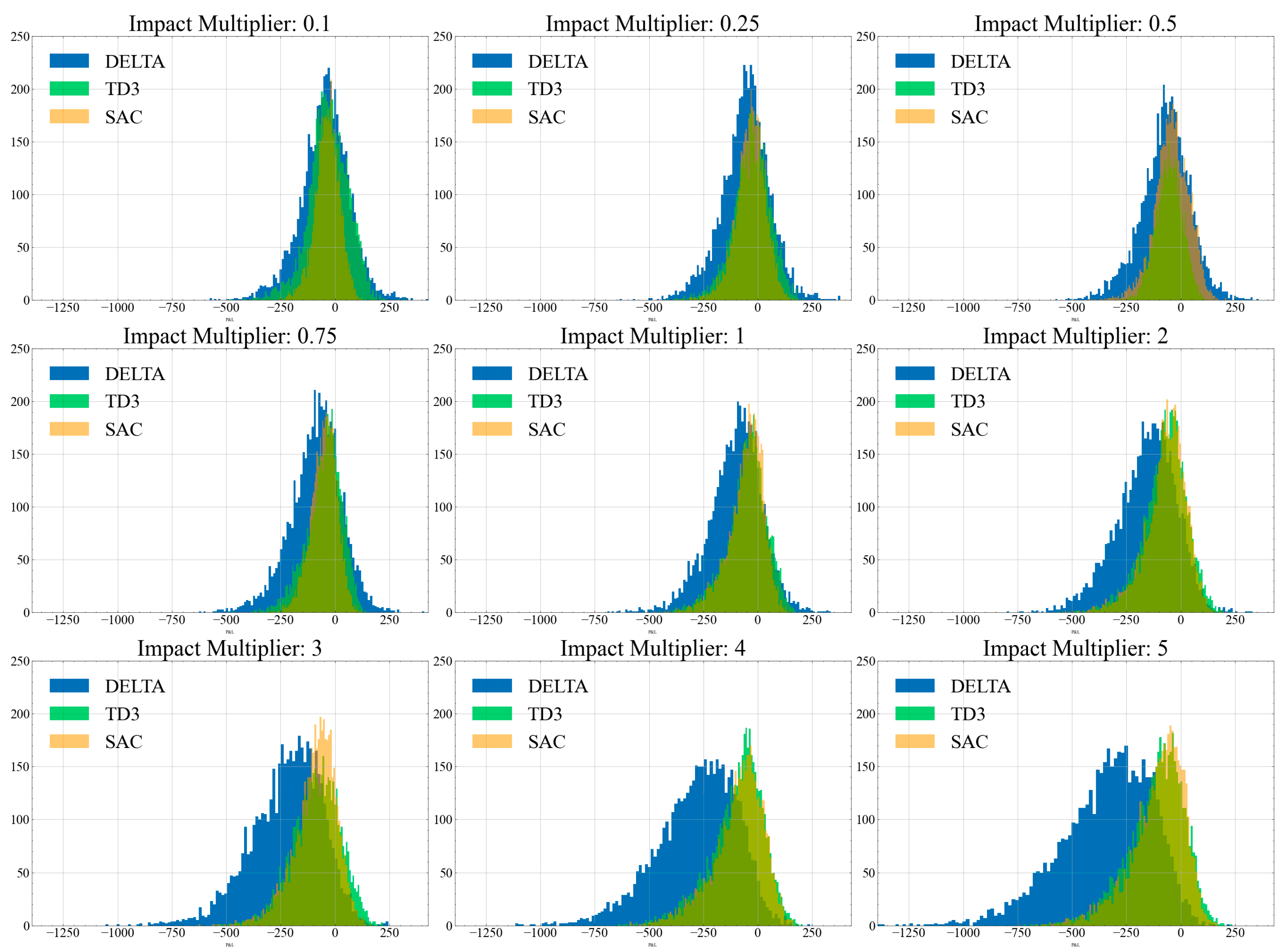Overall, both agents with lower and higher constant transaction costs outperform the benchmarks, with superior risk adjusted performance and total PnL (with the outlier being one agent when $\beta =1,c=0.01).$ The agents consistently achieve a lower CVaR relative to the delta hedging agent, along with lower overall transaction costs; this difference becomes more extreme as the level of $\beta$ increases. We can visualize the difference in Figure 10, which illustrates a histogram of the total PnL across various levels of $\beta$ for the Delta, TD3 and SAC evaluations.

In Figure 11, we can better analyze the learned agentic behaviors in dealing with higher, stochastic slippage costs. Closer to expiry, the agent does not divest its hedged positions as quickly as the benchmark when the option is in-the-money (Figure 11b). However, when the option is out of the money (Figure 11a), we see that the agent liquidates faster than the benchmark strategy; as designed, the temporary impact function encourages faster liquidation to avoid smaller total transaction costs, unlike the delta agent. Although the option expires close to the strike price near the end, the agent decides to liquidate much earlier.

4.4. Temporary and Permanent Market Impact

This section evaluates the performance of reinforcement learning (RL) agents under the most realistic trading conditions, incorporating both temporary market impact ($F$) and permanent market impact (G). These dual frictions create a challenging environment where agents must optimize their hedging strategies to manage short-term deviations in execution price and long-term impacts on the underlying asset’s price path. The results shown below indicate that RL agents vastly excel relative to standard hedging strategies in these scenarios, significantly outperforming the traditional delta hedging benchmark across all evaluation metrics.

We initialize an environment with both permanent and temporary market impact. As outlined by Section 3.1, the total impact M(X″) will be evenly split between permanent impact and temporary impact component, i.e., F(X″) = G(X″) = αM(X″), where α = 0.5 (as defined in Section 3.1). The temporary impact will be reflected in the execution price, seen by the agent through the subsequent reward, while the permanent impact is reflected in the future price path and options value. We analyze the results across various impact magnitudes (β) and decay rates (γ), with a higher constant transaction cost per share of 5 cents. To note, is that compared to experiments in Section 4.3 and Section 4.2, we increase the range of impact multipliers in our environments to account for impact being allocated to both F(X″) and G(X″). Like Section 4.3, we also apply the dynamic volatility model to our environment to account for any large changes in price volatility because of the market impact.

As per Table 4, the RL agents demonstrated robust adaptability by tailoring their trading strategies to account for both temporary and permanent market impacts simultaneously. Unlike prior experiments where the agents focused on a single type of friction, the combined impact environment required the agents to balance competing trade-offs: reducing turnover to mitigate slippage while strategically managing position sizes to minimize the residual effects of permanent impact.

As seen in

Table 5. Permanent Market Impact, Slippage and Transaction Costs, Performance across impact multiplier $\beta$ and permanent impact decay $\gamma$ (10,000 episodes).

Parameters		$\mathbf{Profit}\mathbf{and}\mathbf{Loss}\mathbb{E}$$\left(\mathsf{\Sigma }\mathsf{\Delta }{\mathit{Z}}_{\mathit{t}}\right)$			$\mathbf{Rewards}\mathbb{E}\left(\mathsf{\Sigma }{\mathit{R}}_{\mathit{t}}\right)$			CVaR 0.05			Transaction Costs
β	γ	Delta	TD3	SAC	Delta	TD3	SAC	Delta	TD3	SAC	Delta	TD3	SAC
0.1	0.5	−6.5 ± 112.8	2.2 ± 71.5	3.3 ± 54.5	−1.9 ± 2.8	−0.6 ± 1.0	−0.4 ± 0.7	−215.3	−118.6	−94.6	10.8	9.1	9.6
0.1	1	−7.9 ± 101.1	−3.8 ± 73.6	−4.0 ± 59.8	−1.6 ± 2.5	−0.7 ± 1.1	−0.5 ± 1.0	−165.1	−129.4	−111.3	10.7	8.4	9.7
0.1	2	−10.0 ± 109.3	3.8 ± 64.2	−2.3 ± 59.9	−1.8 ± 2.8	−0.5 ± 0.8	−0.5 ± 0.8	−192.3	−104.5	−103.1	10.9	9.5	9.8
0.25	0.5	−26.0 ± 119.6	−4.8 ± 85.3	−13.4 ± 59.8	−2.2 ± 3.0	−0.9 ± 1.3	−0.6 ± 0.8	−223.9	−129.8	−115.9	10.8	8.5	9.8
0.25	1	−12.7 ± 104.8	−10.8 ± 93.0	−4.2 ± 65.4	−1.6 ± 2.6	−1.1 ± 1.7	−0.6 ± 1.0	−175.9	−169.5	−117.7	10.7	9.1	9.1
0.25	2	−28.8 ± 112.9	−14.2 ± 67.7	−8.0 ± 65.7	−2.3 ± 3.4	−0.6 ± 0.9	−0.5 ± 1.1	−268.3	−129.2	−133.7	10.8	11.2	9.8
0.5	0.5	−20.5 ± 108.3	−7.5 ± 66.7	−18.8 ± 58.0	−1.9 ± 2.5	−0.7 ± 0.9	−0.7 ± 0.8	−216.7	−118.1	−122.3	10.9	8.4	10
0.5	1	−32.2 ± 105.9	−28.0 ± 84.3	−11.5 ± 61.5	−1.9 ± 2.5	−1.2 ± 1.7	−0.6 ± 0.9	−225.8	−176.2	−121.9	10.9	7.8	9.1
0.5	2	−36.7 ± 107.1	−20.0 ± 95.0	−26.6 ± 52.5	−2.2 ± 3.4	−1.4 ± 1.7	−0.6 ± 0.8	−210.1	−177.2	−112.4	11	8.8	10.1
0.75	0.5	−35.0 ± 112.4	−19.2 ± 76.9	−27.1 ± 60.7	−2.0 ± 2.7	−1.0 ± 1.3	−0.8 ± 0.9	−244.2	−135.5	−135.4	10.8	7.9	9
0.75	1	−57.7 ± 109.4	−23.3 ± 84.4	−18.0 ± 57.3	−2.4 ± 3.4	−1.2 ± 1.6	−0.6 ± 0.9	−250.4	−183.7	−118	10.6	8.7	9.3
0.75	2	−40.8 ± 121.9	−25.6 ± 88.4	−27.2 ± 61.6	−2.4 ± 3.2	−1.2 ± 1.5	−0.7 ± 0.8	−250.9	−177.2	−130.1	10.6	7.8	9.5
1	0.5	−78.9 ± 117.0	−26.0 ± 72.4	−37.8 ± 68.7	−3.0 ± 3.8	−1.0 ± 1.1	−1.0 ± 1.1	−303.8	−150.4	−166.2	10.7	8.4	9.4
1	1	−61.5 ± 125.0	−28.1 ± 80.5	−22.5 ± 63.2	−2.8 ± 4.0	−1.1 ± 1.3	−0.7 ± 1.0	−272.4	−171.4	−135.6	10.8	7.7	8.8
1	2	−62.1 ± 114.4	−21.8 ± 91.9	−28.1 ± 61.5	−2.6 ± 3.4	−1.2 ± 1.5	−0.8 ± 1.0	−215.3	−183.4	−94.6	10.8	8.3	8.7

Bolded metrics denote the best performance across Delta, TD3 and SAC across each experiment.

, the RL agents achieved superior performance relative to the benchmark in terms of total hedging PnL and turnover with minimal drawdown risk across varying levels of slippage magnitude and impact persistence. SAC’s achieves the highest mean episodic reward along with the lowest standard deviation in every experiment, which is also reflected in its smaller value at risk compared to the benchmark and TD3. Although TD3 achieves a slightly higher PnL in most experiments, SAC exhibits superior risk management abilities despite having higher transaction costs. This reflects SAC’s optimization for stochastic tasks (such as trading with market impact); the agents likely learned additional patterns in the state space to tamper risks given the algorithm’s entropy maximization.

The agents’ trading behavior reflected a nuanced understanding of the interaction between temporary and permanent impacts. When impact magnitude was substantial, agents adopted a conservative trading approach, limiting large rebalancing trades to avoid compounding costs. By prioritizing minimal turnover, the agents reduced the total impact and slippage costs while maintaining an effective hedge across the episode. As the impact $\beta$ increased, we also see a marked decrease in transaction costs amongst the RL agents relative to Delta, with TD3 trading the least.

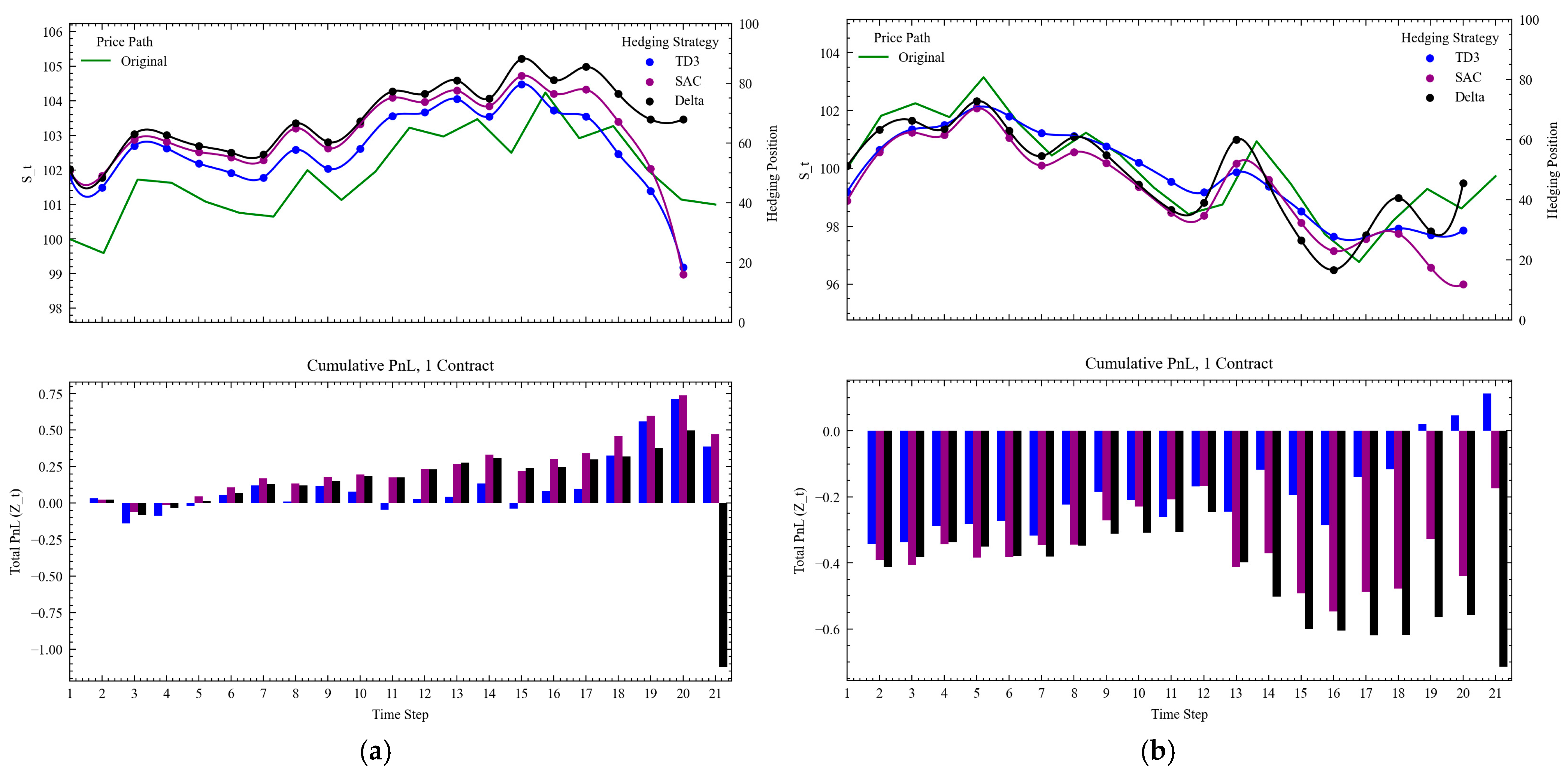
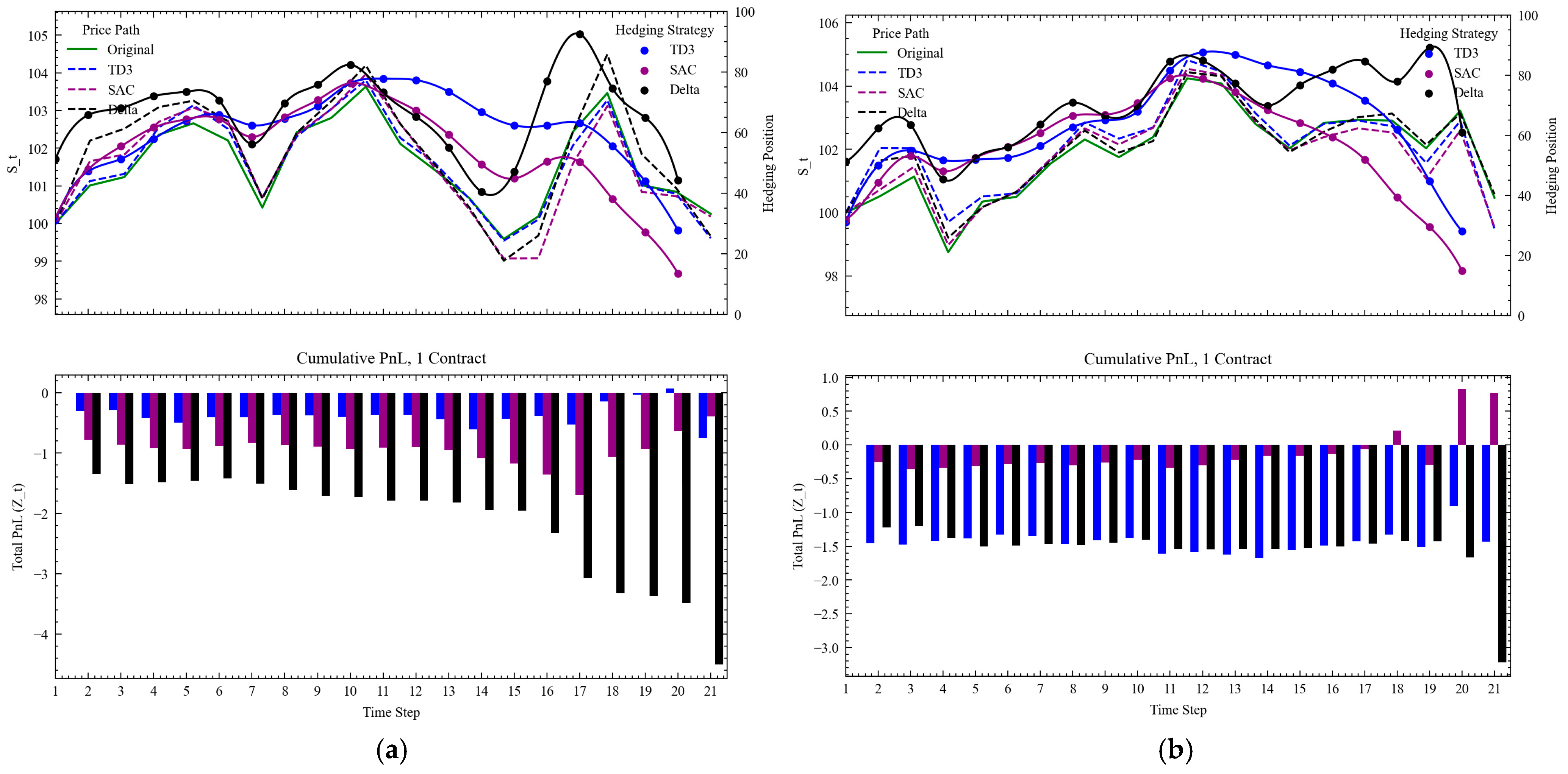
In Figure 12, we can see two specific examples of TD3 the agents hedging an option that expires both in and out of the money. First, across both figures we see that the agents now start at a lower hedging position relative to the delta strategy to reduce total upwards impact of the underlying security. When the option expires in the money (left), we see that the agents learn to decrease their positions substantially prior to expiry to mitigate the volatility spike from a singular trade. We also see that SAC rapidly sells at t = 20, likely to impact the underlying’s price prior to expiry as much as possible to maximize its PnL at the end of the episode. The delta hedging strategy on the other hand holds onto its underlying position and is forced to liquidate at t = 21, resulting in the large PnL drop. Overall, it is interesting to see that the agents are willing to sacrifice early rewards to maximize its rewards at expiry, despite being trained across time steps (rather than episodes). Next, we see that when the trading is against an in-the-money security, the agents slowly liquidate their positions to mitigate against a sudden spike in price (and the costs of overcorrecting their positions).

We conclude that the SAC algorithm is the most suitable for complex hedging environments. These findings highlight the practical applicability of RL-based hedging strategies for institutional traders operating in illiquid or high-cost markets. By optimizing for both immediate and residual costs, the RL agents offer a robust framework for managing derivative portfolios under realistic trading conditions. This capability is particularly valuable for minimizing the combined effects of execution delays and market impact, ensuring cost-efficient and risk-aware portfolio management.

5. Discussion

Our results offer empirical support to the growing body of literature advocating the use of deep reinforcement learning (DRL) for derivative hedging in frictional markets. Similarly to findings by (Buehler et al., 2018; Mikkilä & Kanniainen, 2022), we observe that DRL models not only outperform traditional delta hedging in environments with transaction costs, but also show robust adaptability in the presence of execution slippage and permanent market impact. By constructing an environment where both types of market impact are explicitly modeled—and validated across thousands of simulated paths—we provide a more nuanced and empirically grounded understanding of hedging performance under real-world trading constraints.

Our side-by-side comparison of DDPG, TD3, and SAC across multiple experimental environments distinguishes our work from previous studies which often focus on a single algorithm. For example, while Francois et al. (2025) incorporated market frictions in deep hedging, they primarily evaluated a single agent, making it difficult to generalize findings across algorithm classes. Our comparative analysis shows that TD3 and SAC not only outperform Black–Scholes delta hedging across all experiments but also maintain superior risk-adjusted performance across environments with varying slippage, impact, and transaction costs. DDPG, in contrast, exhibits instability in out-of-sample performance, reinforcing earlier concerns about its reliability in high-variance settings.

SAC’s stochastic policy proves particularly effective in environments with significant stochasticity, as demonstrated in both the temporary and combined impact experiments. It consistently achieves higher PnL and lower CVaR compared to TD3 and DDPG, despite trading more frequently. This challenges the assumption, commonly seen in friction-based literature (e.g., Leland, 1985), that minimizing trades necessarily leads to improved hedging efficiency. Instead, SAC learns to identify and exploit state-dependent opportunities where trading—even with higher transaction costs—yields net performance benefits.

Moreover, our findings expand on the insights from Shi et al. (2024) and Cheridito and Weiss (2025), who explored DRL applications to market making and execution optimization under impact. By contextualizing our results in the broader scope of DRL-based trade execution, we illustrate that our RL agents’ behavior mirrors those of tactical execution agents, strategically delaying or reducing trades in response to liquidity constraints. Our use of a dynamic volatility model further enhances realism by ensuring that agent-induced volatility is penalized appropriately, ensuring learned policies do not exploit arbitrage-like behaviors.

Our experiments also emphasize the importance of environment complexity on model selection. While TD3 performs admirably under simpler transaction cost-only scenarios due to its deterministic policy and bias-reduction mechanisms, it falls short in capturing the adaptive behaviors required under complex frictions. SAC’s entropy-maximizing formulation appears better suited to navigate the multi-modal, stochastic reward landscape introduced by our market impact model, especially under high decay and impact magnitudes.

6. Conclusions

This paper contributes to the literature on deep hedging by presenting a reinforcement learning-based framework capable of adapting to both temporary and permanent market impact, slippage, and transaction costs. Furthermore, we present a comparison of various DRL models across different market impact settings, highlighting the drawbacks and benefits of DDPG, TD3 and SAC in these settings. Our results demonstrate that DRL agents, particularly those utilizing entropy-regularized exploration like SAC, can outperform traditional hedging strategies in both expected return and risk-adjusted terms.

We see that in the most complex experiments with both permanent and temporary market impact, TD3 and SAC can minimize expected losses seen from delta hedging by over 2/3rd (Table 4). SAC specifically illustrated its ability to minimize total value at risk across most experiment parameters, achieving a 50% reduction in CVaR, compared to TD3 with a limited reduction at ~20%. The algorithms’ adaptability across a wide range of environments highlights its potential utility in real-world hedging applications, especially where liquidity constraints and execution costs dominate. Compared to SAC, TD3 also demonstrates reliable performance with faster convergence and efficient trading, making it suitable for lower-friction environments or where training time is a key constraint.

By incorporating realistic cost models and analyzing behavior across frictions, our framework provides a comprehensive testbed for evaluating hedging strategies in markets where trading decisions influence asset prices. The nuanced behaviors observed—such as strategic under hedging, early liquidation, and impact-aware trade timing—illustrate the depth of policy complexity that DRL agents can internalize.

We conclude that actor-critic DRL models, and SAC in particular, offer promising tools for institutional hedging strategies. Their ability to balance risk reduction and cost minimization makes them suitable for illiquid and friction-heavy markets. These findings reinforce the argument for integrating DRL into the risk management toolkits of institutional investors, particularly in portfolios with significant option exposure. Future extensions could include applications to real-world market data, multi-asset portfolios, and integration with execution algorithms for end-to-end portfolio optimization under market impact. Our research contributes to the evolving field of financial risk management by introducing a robust and adaptive DRL-based risk management framework for hedging derivatives under liquidity constraints. The results highlight practical applications of reinforcement learning to improve existing hedging strategies, especially for illiquid instruments sensitive to trade pressure.

7. Limitations and Future Direction

While our findings highlight the potential in the application of deep reinforcement learning frameworks to hedging, there are several areas for future research that could further enhance the applicability and effectiveness of DRL in hedging strategies:

• Application to Real Market Data: Future research should focus on applying the proposed framework to real market data. The agents can be trained with more realistic, security specific transaction cost models as well.
• Expanded Market Factors: Expanding the model to incorporate additional market factors such as macroeconomic indicators, geopolitical events, and sentiment analysis could provide a more comprehensive hedging strategy. Knowledge of these factors can help the model anticipate increased volatility and hedge accordingly.
• Multi-Asset Portfolios: Extending the framework to manage risks in multi-asset portfolios, including FX, bonds, and commodities, could provide broader applicability and more sophisticated risk management capabilities.
• Intraday Trading and Microstructure Analysis: Analyzing the effectiveness of DRL-based hedging strategies in intraday trading scenarios and incorporating market microstructure elements could offer insights into better modelling total expected market impact from hedging. This research would be especially interesting when applied to 0 day to expiry options across various degrees of open interest and market volatility.
• Policy Generalization: Developing transfer learning techniques to enable RL agents trained on one asset or market condition to generalize effectively to others could significantly reduce training time and improve scalability across diverse trading environments.