Abstract
This research seeks to evaluate the effects of the preceding cyclical indicators and macroeconomic variables on the performance of the Brazilian stock market from January 2011 to December 2022. The objective is to identify how these factors influence the behavior of the main index representing this market. In this way, it was analyzed how shocks in the composite leading indicator of the economy (IACE) as well as the basic interest rate of the economy (SELIC), the broad national consumer price index (IPCA), the nominal exchange rate (in reals per dollar—BRL/USD) and the central bank economic activity index (IBC-Br) impact the performance of Brazilian stock market index (IBOVESPA). Using the vector autoregression (VAR) model with vector error correction (VEC), positive shocks were simulated in the IACE and the aforementioned macroeconomic variables to identify and compare their impacts on the index. The results obtained, through generalized impulse response functions, indicated that the shocks to the IACE, the exchange rate, and the inflation variables influenced the IBOVESPA in different and statistically significant ways. However, shocks to the economic activity index and the interest rate did not exert a statistically significant influence on the index, partially confirming the hypothesis, which was initially raised, that these factors influence the stock index in different ways.
1. Introduction
The influence that macroeconomic variables have on the stock market has been a recurring theme in academic research. The studies developed in the Brazilian literature focused on evaluating the influence that the interest rate, inflation, exchange rate and gross domestic product (GDP) have on the IBOVESPA index; however, there is a lack of studies that seek to analyze the impacts that the leading indicators of economic activity, known as cyclical indicators, would have on the performance of the main national stock market index. This topic has become increasingly relevant as studies have been developed in the international literature, such as those by Zhu and Zhu (2014) and Celebi and Hönig (2019), which indicated that cyclical indicators have significant predictive capacity on the performance of different stock indices. They demonstrated that this type of analysis is of great importance for investors in general. In this sense, the present research seeks to fill this gap, adding to the set of variables that can influence the performance of the stock market, the composite leading indicator of the economy (IACE), which is used by the Economic Cycle Dating Committee (CODACE) to determine the economic cycles in Brazil.
Thus, the hypothesis that was tested is that the macroeconomic variables and the preceding cyclical indicators, represented in this study by the IACE, influence the main national stock market index in different ways. Our research analyzed monthly data for the period January 2011 to December 2022, with the objective of comparing the impacts of IACE and macroeconomic variables on the IBOVESPA. In this sense, in addition to the innovative nature of the research, which included a leading indicator to assess the stock market’s behavior, it is worth noting that the Brazilian stock exchange is among the 20 largest in the world and the fourth largest in the Americas, behind only the two stock exchanges in the USA and one in Canada. Therefore, since the selected index is used as a benchmark for the Brazilian stock market, the aim was to find evidence that would help investors, and also companies, to make better decisions when allocating their resources, thus reducing its risks in the face of positive and negative cyclical variations in the Brazilian economy.
To achieve its objectives, this work was divided into six sections. In addition to this first introductory section, Section 2 contains the theoretical framework of the research, presenting the concept of leading economic indicators. Section 3 reviews the empirical literature developed on the topic. Subsequently, Section 4 presents the data and the methodology used, based on the VAR model with error correction, known as VEC. Next, Section 5 analyzes the results obtained by generalized impulse response functions and, finally, Section 6 presents the final considerations.
2. Theoretical Framework
The creation of cyclical leading indicators, or ‘financial barometers’, as they are also known, was inspired by the research of Mitchell (1913). The first of these indicators was Harvard’s ‘ABC’, developed in the 1920s in the United States. However, this financial barometer was unable to anticipate the beginning of the 1929 global crisis and, given its failure to detect it, the indicator was discredited and a decade of stagnation in this area followed. Only with the beginning of a new phase of revitalization of the North American economy in 1938 did new work, aimed at identifying economic cycles, begin to be developed, especially by the National Bureau of Economic Research (NBER), founded by Mitchell in 1920.
During this period, Burns and Mitchell (1946) developed the methodology for a system of leading indicators. For the authors, economic cycles were a type of fluctuation found in the aggregate economic activity of nations with economies based on private companies. These fluctuations were composed of phases of simultaneous expansion in many economic activities and were followed by similar phases of recession, contraction and recovery, which would consolidate with a new phase of expansion in the next cycle. After the authors defined the reference series as the variable whose cyclical movement they sought to anticipate, they constructed a system consisting of three sets of indicators:
- Leading Indicators: Their movements anticipate those of the target variable. Due to their predictive power, they are the most important within the system, serving to signal the behavior of this variable in advance.
- Coincident Indicators: These are those indicators whose fluctuations center on the economic cycle itself, following the movements of the reference variable. They inform movements in the reference series that take time to be announced, more quickly.
- Lagged Indicators: Their movements occur later than those of the target variable. The occurrence of movements in these indicators serves to confirm or rectify what is indicated in the reference series.
However, according to de Oliveira (1991), during a period of rapid economic growth in the 1960s, cyclical analysis received little attention because cycles in the United States’ economy were very smooth or non-existent. Only with the broad recession of 1969–1970, was the topic revitalized, and studies intensified with the advent of the energy crisis. In the early 1970s, researchers at the Center for International Business Cycle Research began an international project to disseminate the NBER methodology to member nations of the Organization for Economic Cooperation and Development (OECD), and to some other countries. Thus, from 1981 onwards, leading and coinciding economic indicators from OECD member countries began to be published regularly in the Economic Indicators Bulletin, seeking to monitor and predict cyclical fluctuations.
In 1995, The Conference Board (TCB), a North American business organization which uses the NBER methodology and measures various time series related to economic activity, was chosen by the US Department of Commerce to produce and distribute a series of leading and coinciding economic indicators that had the capacity to signal the peaks and valleys of American economic cycles. In this way, The Conference Board Leading Economic Index (TCB-LEI) and The Conference Board Coincident Economic Index (TCB-CEI) were created as indicators and began to be published monthly, from February 1996, according to the information contained on the website from TCB (2013).
Therefore, there are two major, globally recognized methods that use the methodology of leading indicators to monitor and anticipate fluctuations in advanced economies: the NBER method (originally developed by Burns and Mitchell in 1920 and currently implemented by the TCB) and the OECD method. The NBER makes efforts to establish a chronology of the peaks and valleys of the economy of the US and 14 other countries associated with the TCB. The OECD method has been used systematically since the end of the 1980s, producing indicators for the economic activity of its member countries.
In the NBER method, the forecast objects are the reversal points, from growth in economic activity to recession and from recession to resumption of growth. Therefore, only the cyclical reversal is anticipated and not the inflection points at which moments of greater or lesser expansion are observed. In this way, the system is built to signal only certain moments of the economic cycle, not its entire trajectory. Any accelerations or decelerations in growth are not captured by the leading indicator, since there is no change in the sign of the reference variable. In the method used by the OECD, the aim is to monitor and predict the cycle as a whole. In this way, even if there are no reversal points or inflection points, the intensification of periods of economic heating or slowdown are captured. Due to this more comprehensive objective, the OECD system is more demanding, in terms of the forecasting capacity of the indicators constructed, which makes it more sensitive to the characteristic errors of leading indicators.
Another important difference between the two systems stands out with respect to the definition of the cycle itself. The NBER method operates with the concept of a cycle in terms of variations in the absolute level of product, with a recession being defined by the continued fall in the level of GDP, visible in industrial production, employment, real income, sales and final consumption. The OECD uses the notion of a growth cycle. This approach is based on the principle that the economy exhibits a positive growth pattern over time, i.e., an economy tends to grow in the long term. Due to this tendency, periods of economic contraction may not manifest themselves through an absolute contraction but only imply a slowdown in growth to a level below the trend. Thus, a boom period would be identified as one in which the observed growth rate is higher than the trend, while a recession is defined as a period in which the economy grows at a rate lower than its potential, the latter being defined by the long-term growth rate. For this reason, the OECD method also requires a statistical calculation of the economy’s growth trend, which constitutes the reference point for identifying a situation of expansion, contraction or recession.
However, despite the divergences between the NBER and OECD methodologies, some requirements are considered to be common. The chosen reference series must be relevant and reliable with respect to the economic cycle. The coinciding series must follow the movements of the target series with a minimum of precision, be subject to little statistical data review and be available in a timely manner.
In Brazil, the Brazilian Institute of Economics (IBRE) of the Getúlio Vargas Foundation, after establishing a partnership with the TCB, created the Economic Cycle Dating Committee (CODACE) in 2009, with the objective of establishing a chronology for past Brazilian economic cycles and futures. In this way, it implemented the NBER methodology. On a monthly basis, CODACE adopts the definition of transition or inflection points in Brazilian business cycles according to classic concepts of expansion and recession but adapted to the characteristics of the Brazilian economy. To this end, the committee developed two cyclical indicators: the composite leading indicator of the economy (IACE) and the composite coincident indicator of the economy (ICCE), according to information contained in the Announcement on the Creation of CODACE and Dating of Brazilian Quarterly Cycles, released in May 2009.
Figure 1 shows that the composite economic leading indicator (in orange) showed significant predictive capacity in relation to the behavior of the economic activity index (in black), indicating both the contraction that the Brazilian economy suffered from March 2014 to December 2016 and the expansion that occurred from January 2017 to December 2021 in advance.
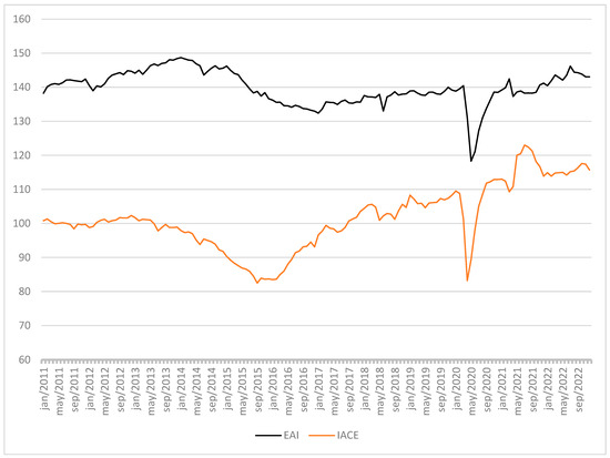
Figure 1.
Comparison between the economic activity index (EAI) and the composite leading indicator of the economy (IACE) from January 2011 to December 2022. Source: Prepared by the authors. Data available in https://ciclo-economico-ibre.fgv.br/ (accessed on 25 November 2022).
3. Empirical Literature Review
Studies that are aimed at analyzing the relationships between cyclical indicators of economic activity and the stock market have been concentrated in the international literature. It was observed that most of these studies focused on antecedent and coincident economic indicators developed by the OECD; however, it is possible to find works that opted for the cyclical indicators prepared by the TCB.
Among the research that used OECD indicators, the work of Zhu and Zhu (2014) stands out, in which the authors identified the significant predictive capacity of a cyclical indicator preceding the OECD, the European leading economic indicator (OECD-ELEI), in relative to stock returns in 12 European countries. Using a multiple regression model, the authors analyzed the returns of these countries’ indices during the period 1980 to 2013 and found that the predictive capacity of the OECD-ELEI, in relation to stock returns, was much higher than that of the national leading indicator from the OECD, the country leading economic indicator (OECD-CLEI).
In this sense, Celebi and Hönig (2019) evaluated the impact of cyclical and macroeconomic indicators in Germany, such as the OECD composite leading indicator (OECD-CLI), the business confidence index (BCI), the consumer confidence index (CCI) and the yield of German government bonds, on the performance of the country’s main stock index (the DAX30), during the period 1991 to 2018. The authors divided the study period into pre-crisis, crisis and post-crisis periods and carried out different regressions; they identified that, among all the indicators analyzed, the OECD-CLI was the one that presented the greatest explanatory power for the behavior of the DAX30, according to the lr-test and the R-square. Therefore, they concluded that, in periods of crisis, asset managers and investors in general should pay more attention to trends in classic macroeconomic variables, especially leading economic indicators such as the OECD-CLI.
In relation to studies aimed at measuring the effects of macroeconomic variables on stock markets, there is a large amount of work with this focus at an international level. One of the pioneering works was by Chen et al. (1986), who investigated the effect of several variables on stock returns. Using the monthly returns of North American stocks over the period 1958–1984, the authors employed the arbitrage pricing theory (APT) structure and observed that a positive variation in industrial production, the risk premium and the term structure of the interest rate had a positive impact on stock returns, while a rise in the expected inflation rate or unexpected inflation had a negative relationship with stock returns, due to its impact on future dividends and the discount rate.
Another work that focused on the American stock market was prepared by Lee (1992). The author analyzed the causal relationship and dynamic interactions between the stock returns of the New York Stock Exchange index (NYSE), the real interest rate (IRE), the industrial production level (IPG) and the inflation rate (INF) in the post-war period, between January 1947 and December 1987. To do this, he used the VAR approach and examined the validity of the model that explained the negative relationship between the increase in the inflation rate and stock returns. The results found were compatible with those found in the study by Fama and French (1996).
Expanding the analysis of the effects of macroeconomic variables on other American stock market indices, Lin et al. (2022) investigated the effects of the gross domestic product (GPD), consumer price index (CPI), price index to the producer (PPI), unemployment rate (UNRATE), Oil Prices (OIL) and effective funds rate (EFFR) on the Dow Jones, S&P 500 and NASDAQ indices, between January 2011 and December 2021. The authors carried out a regression between each of the stock indices and the selected variables, and they found that the unemployment rate and the effective funds rate were the two variables that had the greatest influence on the indices. The results also revealed that the CPI had a negative impact on the three indices, while the GDP did not demonstrate a relative effect on the analyzed indices.
In the national literature, the work of de Souza Grôppo (2005) stands out as the first in Brazilian literature to discuss the causal relationship between macroeconomic variables and the IBOVESPA through the VAR model. The author analyzed the causal relationship between macroeconomic variables, the short-term interest rate (Selic), the real exchange rate (PTAX), the price of a barrel of oil on the international market (PET) and the industrial production index (PROD) on the IBOVESPA. The results obtained demonstrated that the Brazilian stock index has a high sensitivity to interest rates. Furthermore, the study identified that increases in short-term interest rates and exchange rates negatively affect the index, as do unexpected shocks in the price of oil.
De Carvalho and Sekunda (2020) analyzed whether the interest rate and GDP had a long-term relationship with the return of the Brazilian stock market. Using a VEC model, the authors carried out a co-integration and causality test between the IBOVESPA and IBRX-100 index series, with the DI, Selic and PIB series, from January 1997 to December 2018. The results obtained demonstrated the existence of co-integration vectors between the variables, as well as the statistically significant influence of the DI short-term interest rate on the return of the indices, just as de Souza Grôppo (2005) had found in his study. However, the Selic and GDP variables were not statistically significant for the IBOVESPA and IBRX-100 series in the long term; nor did the Granger test indicate that any of these variables presented a causal relationship with the stock index series.
Vartanian et al. (2022) evaluated the influence of inflation, the exchange rate, the industrial production index, the interest rate and the price of international oil on the IBOVESPA. The authors used the VEC methodology and, using impulse response functions, simulated how shocks to these variables influenced the behavior of the index. The results indicated that IBOVESPA has a significant negative relationship with the exchange rate and interest rate but a positive relationship with economic activity, especially with the growth of industrial production.
4. Data and Methodology
The present work sought to include a cyclical indicator that precedes the literature that evaluates the factors that influence the stock market in Brazil. In this sense, the Composite leading indicator of the economy (IACE) was selected due to its significant ability to anticipate cyclical fluctuations occurring in Brazilian economic activity, according to information contained on the website of the Economic Cycle Dating Committee (CODACE—FGV-IBRE, 2009). Regarding the selection of macroeconomic variables used, it was based on a review of national literature, where it was identified that the factors most used in works developed on the subject were inflation, the interest rate, the exchange rate and the GDP. Thus, the analysis contributes to the inclusion of a new variable, the leading cyclical indicator, in a set of studies that sought to assess the factors that influence the stock market in Brazil. In addition to the leading cyclical indicator, the selection of macroeconomic variables was based on the primary studies carried out on the subject, presented previously in the theoretical framework. It is worth noting that the Brazilian stock exchange is the largest in Latin America, the fourth largest in the Americas, behind the two stock exchanges in the USA (NYSE and NASDAQ) and Canada (TSX), and is among the 20 largest stock exchanges in the world, with emphasis on the fact that Brazil is part of the group of emerging countries, which reinforces the importance of analyzing the influence of leading indicators on the behavior of the stock market together with the macroeconomic variables applied in the main research on the subject.
Therefore, the variables incorporated into the econometric model proposed in this study used monthly series and were obtained from the following databases:
- Leading Cyclical Indicator: The composite leading indicator of the economy (IACE) was represented in the model by the variable (EA) and its monthly series were extracted from the database of the Brazilian Institute of Economics FGV-IBRE (2009).
- Interest Rate: The economic basic interest rate (SELIC) was adopted in the model as a variable (IR) and its monthly series were extracted from the database of the Central Bank of Brazil.
- Inflation: The broad national consumer price index (IPCA) was represented by the variable (INF) and its monthly series obtained from the Economática platform.
- Exchange Rate: The Express Nominal Exchange Rate, BRL/USD, was used as the variable (ER) and its monthly series extracted from the Central Bank of Brazil.
- Gross Domestic Product: The central bank economic activity index (IBC-Br) represented the variable (GDP) in the model and its monthly series were extracted from the Central Bank of Brazil (IBC-Br—with seasonal adjustment (2002 = 100)).
- IBOVESPA: The Brazilian stock index (IBOVESPA) was represented in the model by the variable (IBOVESPA) and its series were extracted from the Economática platform.
Table 1 presents the main descriptive statistics of the survey, bringing together the IBOVESPA index, the cyclical indicator and the selected macroeconomic variables.

Table 1.
Descriptive statistics of the variables between January 2011 and December 2022.
It was observed that the IBOVESPA showed a large fluctuation during the analyzed period, with a minimum price of 40,405 points and a maximum score of 126,801 and, therefore, an average of 75,378 points. Figure 2 presents graphs showing the evolution of the variables analyzed over the period considered by the study.
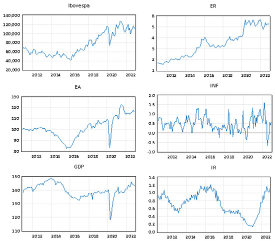
Figure 2.
Evolution of variables from January 2011 to December 2022. Source: prepared by the authors based on the econometric package E-views 12.
Regarding the econometric model, it was initially intended to use a vector autoregressive (VAR) model, pioneered by Sims (1980), which appears to be an alternative to multi-equational models, as it eliminates the need to impose a priori restrictions, with possible harm to the analysis of information, as demonstrated by Sims (1986). According to the author, the VAR model would enable the analysis of the variables listed above simultaneously, in order to avoid the problems of identifying parameters in multi-equational models.
Therefore, the impulse response function (FIR) was used as a comparative analysis instrument, since this function allows the simulation of specific shocks in each of the model’s variables. As these shocks dissipate through the other variables through the structure of the VAR model itself, it is possible to estimate the impact on the variables and predict how this impact will be felt in the future. Based on these estimates, it was possible to visualize the dynamic behavior of the IBOVESPA in the face of any change in the cyclical indicator and in the macroeconomic variables used in this study, thus capturing the change in the behavior of the index at the time when another variable or the analyzed index itself suffers a shock at time t, by replicating this impulse into the future (in periods t+1, t+2, and so on). It is important to highlight that the variables leading cyclical indicator, exchange rate, gross domestic product and IBOVESPA underwent logarithmic transformation. In contrast, the inflation and interest rate variables were not precisely transformed into logarithms because they were already expressed as rates. For this reason, the shocks analyzed and interpreted in the impulse response functions presented below can be interpreted based on the concept of elasticity.
The mathematical formula of the VAR model, according to Gujarati and Porter (2011), is represented in Equation (1):
where
- = endogenous variable vector;
- = exogenous variable vector;
- = matrices of coefficients to be estimated;
- = self-correlated innovation vector.
The VAR model’s main characteristic is the explanation of variables by the past of the variable itself, as well as by the past of the other variables in the model. Therefore, the main objective of this research was to evaluate how the performance of IBOVESPA responded to impulses (positive shocks) on the leading cyclical indicator IACE and on the macroeconomic variables interest rate, inflation, exchange rate and economic activity index. The generalized impulse response function was used because of its ability to simulate the impacts necessary to generate the desired results in the general objective of the work.
According to Hill et al. (2011), the VAR model requires stationary variables. The term ‘stationary’ is understood to mean a series whose statistical mean and variance are the same over time and the covariance between two values in the series only depends on the time that separates them, with no restriction on the correlation between the variables, i.e., they may or may not be correlated with each other. That said, according to Granger and Newbold (1974), when the series do not present stationarity, a VEC model must be estimated, since non-stationary macroeconomic series can cause the problem of spurious regression. For this reason, Maysami and Koh (2000) suggested the application of an error correction term, so that the behaviors of short-term variables are adjusted in line with long-term behaviors.
The combination of the VAR model with an error correction term makes it possible to apply a vector autoregressive model with error correction (VEC), through the formation of linear combinations of stationary integrated variables (co-integrated). In this case, the co-integration of two series (e.g., Xt and Yt) leads to an equal or common stochastic trend, by eliminating the difference Yt − θXt. In this way, the co-integration of these two series makes it possible to model the respective first differences using VAR, with the addition of an additional regressor, the error correction term, which is Yt−1 − θXt−1. Therefore, it becomes possible to estimate predictions of future values of ΔYt and ΔXt, based on past values of Yt − θXt.
In this sense, before applying the VEC model, it was necessary to identify possible co-integration vectors between the series used. To this end, Johansen’s (1988) co-integration test was performed to estimate the presence and quantity of these vectors. In the present research, the results obtained in the co-integration testjustify the use of the VEC model, just as Mukherjee and Naka (1995) did in their research. The authors applied the VEC model to a system of seven equations, with the objective of evaluating the co-integration between the Japanese stock market and six macroeconomic variables. Based on the results obtained, Mukherjee and Naka (1995) concluded that the VEC model consistently outperforms the VAR model, in terms of predictive capacity.
Furthermore, according to Gujarati and Porter (2011), the application of the VEC model has the advantage of not requiring a priori assumptions, which normally occur if the model’s regressors are correlated with the error, generating endogeneity problems. Therefore, in mathematical terms, a hypothetical system of two variables and a co-integration equation presents the following algebraic formula:
The resulting VEC model has the following equations:
Equations (3) and (4) present the error correction term, which is equivalent to zero in the long-term equilibrium, although, in the short term, the variables may be suitable for the long-term equilibrium according to the speed of adjustment of endogenous variables, expressed by the coefficients and y1, y2, a1, a2.
In this sense, given the presence of originally non-stationary series that can be co-integrated, it is necessary to estimate the VEC model with the detection of the co-integration equation and with the appropriate number of lags. Thus, to find the best information criterion, simulations were carried out, considering the number of co-integration equations found with different lags, in order to select the most parsimonious model according to the criteria of Akaike (1974) and Schwarz (1978). Table 2 shows the results found for each of the lags applied:
Table 2.
Information criteria of Akaike (1974) and Schwarz (1978) for the model.
Johansen’s (1988) co-integration test has the null hypothesis of the absence of co-integration vectors, while the alternative hypothesis indicates that there is at least one co-integration vector. Given the fact that, with the exception of the INF variable series, all other series proved to be non-stationary, co-integration tests were carried out, with a constant trend, in order to find the number of co-integration equations present. Therefore, according to the results presented in Table 3, the Johansen test applied ensured the use of the VEC model with two lags and one co-integration equation, refuting the null hypothesis and ensuring the best adequacy of the VEC model to the selected variables.
Table 3.
Results of the Johansen co-integration test with 2 lags.
Maysami and Koh (2000) highlighted the need to analyze the stability of the models through the inverse roots of the characteristic autoregressive polynomial. In this sense, Figure 3 shows that the estimated model demonstrated stability because all of its roots lie within the unit circle.
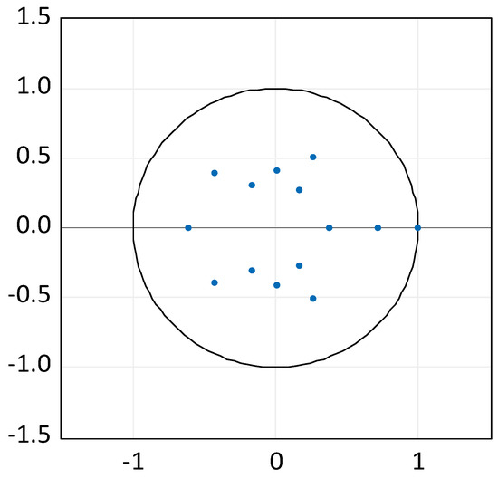
Figure 3.
Inverse roots of AR polynomial feature. Source: author’s own elaborations on econometric data.
To check the presence of autocorrelation, the portmanteau autocorrelation test was performed, in which the null hypothesis is the absence of autocorrelation. The results can be seen in Table 4. It is highlighted that the test is only valid for lags greater than the model’s lag order.
Table 4.
Portmanteau test for the IBOVESPA model.
Another of the tests carried out was residual heteroskedasticity test without crossed terms, just levels and squares, with 155 observations between January 2011 and December 2022, as shown in Table 5. It is worth highlighting that the model estimated in this research used financial series. Therefore, the presence of heteroscedasticity is common, which was confirmed by the test results, both in terms of individual components and the joint test case.
Table 5.
Residual heteroscedasticity test of the IBOVESPA model.
One way to minimize the heteroscedasticity identified was the logarithmic transformation of the variables, which mitigated its effects but did not completely eliminate it, as can be seen from the results in Table 5. However, as the objective of the present work was to analyze the functions of impulse response, it is worth highlighting that heteroscedasticity changes the standard deviations of the variables but not the estimated coefficients. Therefore, its presence in the residues did not harm the estimates and the consequent analysis of the impulse response functions.
5. Results and Discussion
Using the econometric package in the E-views 12 software, impulse response functions were generated to simulate a hypothetical shock of one standard deviation in the leading cyclical indicator (EA_L), the exchange rate (ER_L), the economic activity (GDP_L), inflation (INF) and Selic rate (IR), to see if they could influence the behavior of IBOVESPA within a 6-month horizon. It is important to highlight that, in order to reduce possible differences in the results resulting from the ordering of the variables, the present research used generalized impulse response functions to the detriment of ordering, based on the Cholesky method.
Figure 4 shows the impulse response functions on the IBOVESPA. It is observed that the index responded in a similar way to shocks in the cyclical indicator (EA_L) and in the economic activity index (GDP_L); however, as the horizontal axis lies within the 95% confidence interval (represented by the red lines), it was not possible to conclude whether the responses to the two factors were really similar. However, it is worth highlighting that, if the confidence interval is not considered, IBOVESPA’s response to a shock to (EA_L) remained positive throughout the period, while the index’s response to the shock to the economic activity index (GDP_L) was initially positive but became negative. Therefore, it was not possible to define what effect this variable had on the index.
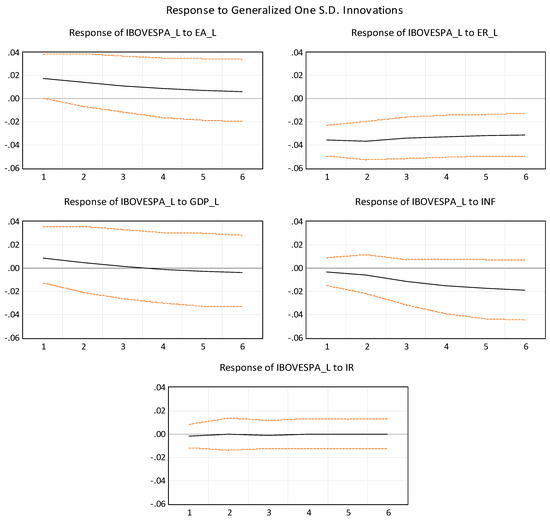
Figure 4.
Generalized impulse response functions with one-standard deviation shocks. Source: prepared by the authors based on the econometric package E-views 12.
Regarding the index’s response to an exchange rate shock (ER_L), it was found that the IBOVESPA presented a negative response for the entire period considered; therefore, this was the variable that had the greatest influence on the index among all the variables considered in the study. This negative response of IBOVESPA to an exchange rate shock corroborates the results found in the research by de Souza Grôppo (2005). As for the response of the index to inflation (INF), it was found that it was negative throughout the analyzed period. Regarding the response of the index to the interest rate (IR), it was found that this variable did not exert a statistically significant influence on the IBOVESPA, which diverged from the results obtained by de Souza Grôppo (2005) but converged with the findings in De Carvalho and Sekunda (2020).
Table 6 presents a summary of the responses presented by IBOVESPA, given the shocks in the cyclical indicator and macroeconomic variables.
Table 6.
IBOVESPA responses to shocks in variables.
Based on the results presented in Table 4, it can be seen that, when faced with a shock to the leading cyclical indicator (IACE), the IBOVESPA’s response in the exchange rate and in inflation (IPCA) were very different from each other. Regarding the shock to the economic activity index (IBC-Br), it can be seen that the response proved to be undefined, i.e., it was not possible to conclude whether the IBC-Br exerts a positive or negative influence on the index. Regarding the shock to the interest rate (Selic), it was found that a shock to this variable did not have an influence on the index.
Therefore, the initial research hypothesis can be partially confirmed, since the leading cyclical indicator, exchange rate and inflation influenced the IBOVESPA in different ways. However, the influence exerted by the economic activity index on the stock index cannot be defined and the influence of the interest rate was shown to not be statistically significant. Therefore, this work identified three variables that have a significant influence on the performance of the index used as a benchmark for national stock markets: the composite leading indicator of the economy (IACE), the nominal exchange rate (BRL/USD) and the broad consumer price index (IPCA).
The composite leading indicator of the economy (IACE) is made up of eight economic indicators that have their values changed before a trough or a peak in economic activity; therefore, each of them has a significant predictive capacity to anticipate an expansion or contraction in the GDP. By comparing the response of the IBOVESPA to a shock to this variable, with the responses of the index to the other variables, it appears that the IACE was the only one that influenced the IBOVESPA in a positive way. The positive response was immediate, and it then decreased within months, which highlights the high sensitivity of the index, given the economic expectations that a cyclical indicator aims to anticipate. Therefore, as Celebi and Hönig (2019) concluded, in periods of crisis, asset managers and investors in general should pay more attention to trends in classic macroeconomic variables, especially in leading economic indicators.
The nominal exchange rate (BRL/USD) expresses the value relationship between the Brazilian real and the American dollar; this rate is determined by several factors, such as exchange rate policy, trade balance, foreign investments and tourism. Therefore, the behavior of this variable presents a characteristic of great unpredictability, which increases its power of influence over different sectors of the economy. This characteristic is evident in the results obtained in this study, since the exchange rate was the variable that exerted the greatest negative influence on the IBOVESPA. It was observed that the index showed greater sensitivity to an exchange rate shock and the response was of greater intensity compared to the index’s responses to shocks to other variables. This result differed from those obtained by de Souza Grôppo (2005), who identified the interest rate as the variable that exerts the greatest negative influence on the index.
The broad consumer price index (IPCA) is one of the main inflation indices in Brazil, calculated by the Brazilian Institute of Geography and Statistics (IBGE), and is also known as the index that measures official inflation in the country. Regarding this variable, the results found in this research demonstrated that the IPCA also exerted a negative influence on the IBOVESPA but with a lower intensity when compared to the exchange rate. The negative response of the index to a shock to the IPCA became increasingly negative over the months but with a smaller amplitude, in relation to the exchange rate shock. This result differed from that found by Vartanian et al. (2022), as the authors identified a negative response from the IBOVESPA in the first three months, which then became positive between the fourth and sixth months and, finally, returned to being negative in the remainder of the period.
6. Conclusions
This article sought to analyze how the antecedent cyclical indicator (IACE) and the macroeconomic variables (interest rate, inflation, exchange rate and economic activity index (IBC-Br)) influenced the performance of Brazilian stock markets during the period January 2011 to December 2022. To achieve this objective, the research used the IBOVESPA quotation series, Brazil’s main stock index, and employed the vector autoregressive model (VAR) with error correction, known as the VEC model, due to the identification of non-stationary series.
After carrying out all the tests indicated by the applied methodology, a VEC model was estimated and so, we proceeded with the elaboration of the impulse response functions, in which shocks were carried out on the IACE indicator and the macroeconomic variables, with the objective of analyzing the influence of these shocks on the stock index. The results obtained demonstrated that the shocks to the leading cyclical indicator, the exchange rate and inflation influenced the indexes in different ways, while the shocks to the IBC-Br and the interest rate did not exert a defined and significant influence on the IBOVESPA. Therefore, the research hypothesis that the stock market is influenced in different ways by cyclical and economic factors has been partially confirmed, since three of the five factors considered influenced the IBOVESPA in different ways, while two did not exert a statistically significant influence.
It is important to highlight the fact that, of the five variables analyzed, the exchange rate (ER_L) was the one that exerted the greatest influence on the index, a result that converges with the findings in Vartanian (2012). Furthermore, the elasticity presented by the index in the face of an exchange rate shock was double, when compared to the elasticity presented by the index in the face of an inflation shock.
Therefore, as the index presented different responses to most of the simulated shocks, the main contribution of this research is to expand the analytical capacity of investors who seek to diversify and protect their investment portfolios, in the face of uncertainties and constant changes in the Brazilian macroeconomic scenario. Another contribution that deserves to be highlighted is the inclusion of the composite economic leading indicator (IACE) as one of the factors that can influence the performance of stock markets. In this sense, based on the results presented, investors and companies will be able to identify how the cyclical indicators that make up the IACE can affect the main national stock index.
As for the limitations of this research, it is important to highlight the number of observations of the series used. As the VEC models estimated in this work have many parameters, it is recommended to use time series with the largest number of observations possible, so that the explanatory capacity of the model is reliable. From this perspective, the number of observations was limited by the IFIX and IACE series, since both began in January 2011. Another limiting factor that deserves to be mentioned is the lack of research investigating the influence of the leading indicator on the financial indexes in Brazil; the existing work in this area is concentrated in the international literature.
In relation to future research, we suggest that the reasons why the interest rate (IR_L) did not have a statistically significant influence on the IBOVESPA should be investigated because this result diverged from that found by de Souza Grôppo (2005).
Author Contributions
All authors contributed equally to this work, P.R.V. and R.L.G. All authors have read and agreed to the published version of the manuscript.
Funding
The APC was funded by Mackenzie Presbyterian University.
Institutional Review Board Statement
Not applicable.
Informed Consent Statement
Not applicable.
Data Availability Statement
The original data presented in the study are openly available in [Zenodo] at [https://doi.org/10.5281/zenodo.14778970].
Conflicts of Interest
The authors declare no conflict of interest.
References
- Akaike, H. (1974). A new look at the statistical model identification. IEEE Transactions on Automatic Control, 19(6), 716–723. [Google Scholar] [CrossRef]
- Burns, A. F., & Mitchell, W. C. (1946). The basic measures of cyclical behavior. In Measuring business cycles (pp. 115–202). National Bureau of Economic Research. [Google Scholar]
- Celebi, K., & Hönig, M. (2019). The impact of macroeconomic factors on the German stock market: Evidence for the crisis, pre-and post-crisis periods. International Journal of Financial Studies, 7(2), 18. [Google Scholar] [CrossRef]
- Chen, N.-F., Roll, R., & Ross, S. A. (1986). Economic forces and the stock market. Journal of Business, 59(3), 383–403. [Google Scholar] [CrossRef]
- CODACE—FGV-IBRE. (2009). Comitê de datação de ciclos econômicos. Rio de Janeiro. Available online: https://portalibre.fgv.br/sites/default/files/2020-03/comite-de-data_o-de-ciclos-econ_micos-ibre-fgv-27.05.09.pdf (accessed on 1 November 2022).
- De Carvalho, P. L., & Sekunda, A. (2020). Influência das variáveis macroeconômicas sobre desempenho do mercado de capitais brasileiro. In Anais da 20ª USP international conference in accounting. USP. [Google Scholar]
- de Oliveira, E. G. (1991). Ciclos econômicos-indicadores. Revista Conjuntura Econômica, 45(9), 81–84. [Google Scholar]
- de Souza Grôppo, G. (2005). Relações Dinâmicas entre um Conjunto Selecionado de Variáveis Macroeconômicas e o IBOVESPA. Revista de Economia e Administração, 4(4), 445–464. [Google Scholar]
- Fama, E. F., & French, K. R. (1996). Multifactor explanations of asset pricing anomalies. The Journal of Finance, 51(1), 55–84. [Google Scholar] [CrossRef]
- Granger, C. W. J., & Newbold, P. (1974). Spurious regressions in econometrics. Journal of Econometrics, 2(2), 111–120. [Google Scholar] [CrossRef]
- Gujarati, D. N., & Porter, D. C. (2011). Econometria básica (5th ed.). Amgh Editora. [Google Scholar]
- Hill, R. C., Griffiths, W. E., & Lim, G. C. (2011). Principles of econometrics (4th ed.). Wiley. [Google Scholar]
- Johansen, S. (1988). Statistical analysis of co-integration vectors. Journal of Economic Dynamics and Control, 12(2–3), 231–254. [Google Scholar] [CrossRef]
- Lee, B.-S. (1992). Causal relations among stock returns, interest rates, real activity, and inflation. The Journal of Finance, 47(4), 1591–1603. [Google Scholar] [CrossRef]
- Lin, G., Vecchio, A., Yager, E., & Liu, W. (2022). Macroeconomic factors and stock market indices. International Journal of Business and Economics, 7(1), 230–242. [Google Scholar] [CrossRef]
- Maysami, R. C., & Koh, T. S. (2000). A vector correction model of the Singapore stock market. International Review of Economics & Finance, 9(1), 79–96. [Google Scholar]
- Mitchell, W. C. (1913). Business cycles. University of California Press. [Google Scholar]
- Mukherjee, T. K., & Naka, A. (1995). Dynamic relations between macroeconomic variables and the Japanese stock market: An application of a vector error correction model. Journal of Financial Research, 18(2), 223–237. [Google Scholar] [CrossRef]
- Schwarz, G. (1978). Estimating the dimension of a model. The Annals of Statistics, 6(2), 461–464. [Google Scholar] [CrossRef]
- Sims, C. A. (1980). Macroeconomics and reality. Econometrica, 48(1), 1–48. [Google Scholar] [CrossRef]
- Sims, C. A. (1986). Are forecasting models usable for policy analysis? Federal Reserve Bank of Minneapolis Quarterly Review, 10(1), 2–16. [Google Scholar] [CrossRef]
- The Conference Board. (2013). Press release FGV/IBRE—TCB. Rio de Janeiro. Available online: https://www.conference-board.org/pdf_free/translations/011714.pdf (accessed on 3 November 2022).
- Vartanian, P. R. (2012). Impactos do índice dow jones, commodities e câmbio sobre o IBOVESPA: Uma análise do efeito contágio. Revista de Administração Contemporânea, 16, 608–627. [Google Scholar] [CrossRef]
- Vartanian, P. R., dos Santos, H. F., da Silva, W. M., & Fronzaglia, M. (2022). Macroeconomic and financial variables’ influence on Brazilian stock and real estate markets: A comparative analysis in the period from 2015 to 2019. Modern Economy, 13(5), 747–769. [Google Scholar] [CrossRef]
- Zhu, Y., & Zhu, X. (2014). European business cycles and stock return predictability. Finance Research Letters, 11(4), 446–453. [Google Scholar] [CrossRef]
Disclaimer/Publisher’s Note: The statements, opinions and data contained in all publications are solely those of the individual author(s) and contributor(s) and not of MDPI and/or the editor(s). MDPI and/or the editor(s) disclaim responsibility for any injury to people or property resulting from any ideas, methods, instructions or products referred to in the content. |
© 2025 by the authors. Licensee MDPI, Basel, Switzerland. This article is an open access article distributed under the terms and conditions of the Creative Commons Attribution (CC BY) license (https://creativecommons.org/licenses/by/4.0/).