News Sentiment and Stock Market Dynamics: A Machine Learning Investigation

Abstract

The study relies on an extensive dataset (≈1.86 million news headlines) to investigate the heterogeneity and predictive power of explicit sentiment signals (TextBlob, VADER, and FinBERT) and implied sentiment (VIX) for stock market trends. We find that news content predominantly consists of objective or neutral information, with only a small portion carrying subjective or emotive weight. There is a structural market bias toward upswings (bullish market states). Market behavior appears anticipatory rather than reactive: forward-looking implied sentiment captures a substantial share (≈45–50%) of the variation in stock returns. By contrast, sentiment scores, even when disaggregated into firm- and non-firm-specific subscores, lack robust predictive power. However, weekend and holiday sentiment contains modest yet valuable market signals. Algorithm-wise, Gradient Boosting Machine (GBM) stands out in both classification (bullish vs. bearish) and regression tasks. Neither FinBERT news sentiment, historical returns, nor implied volatility offer a consistently exploitable edge over market efficiency. Thus, our findings lend empirical support to both the weak-form and semi-strong forms of the Efficient Market Hypothesis. In the realm of exploitable trading strategies, markets remain an enigma against systematic alpha.

1. Introduction

The interplay between information flow and market behavior has long intrigued economists and behavioral scholars. In today’s digital era, news spreads instantly, making sentiment analysis more relevant than ever. Understanding how sentiment in text influences market dynamics is a growing area of interest. Traditional stock price models, grounded in the Efficient Market Hypothesis (EMH), argue prices reflect all known data (Fama, 1970). This leaves little theoretical room for emotions or tone to influence asset prices. Yet growing empirical evidence shows investor sentiment can move prices beyond fundamentals. News reactions, whether optimistic, pessimistic, or neutral, can sometimes shape short-term market swings. This study asks whether sentiment scores from TextBlob, VADER, and FinBERT predict such movements. In doing so, it aims to link qualitative narratives in financial news to real, measurable market behavior.

The motivation for this investigation stems from the rise of unstructured textual data and NLP advancements. Earlier studies showed that earnings announcements and macro news impact returns, often with delayed effects (Ball & Brown, 1968). These early works were mainly event-based, overlooking the steady stream of sentiment in daily news cycles. Recent research shifted to sentiment analysis to bridge this gap in market reaction studies. For example, Bollen et al. (2019) showed Twitter sentiment predicts cryptocurrency prices. Similarly, Tetlock and Saadi (2020) linked news sentiment indices with short-term equity volatility. Still, the literature remains divided on whether sentiment offers real signals or just reflects noise (Garcia & Norli, 2021). This paper uses TextBlob, VADER, and FinBERT to rigorously test sentiment’s predictive value in a replicable framework, especially in the context of any exploitable trading signal.

Beyond academic curiosity, decoding news sentiment holds significant practical value. Portfolio managers, traders, and policymakers increasingly seek real-time signals during turbulent periods. The pandemic-driven market swings of 2020 revealed how “animal spirits” can override fundamentals (Shiller, 2020). Chen et al. (2022) showed sentiment shaped trading volumes during COVID-19, while Li et al. (2023) found it predicted tech stock returns. TextBlob, VADER, and FinBERT offer distinct yet complementary tools to analyze sentiment’s role. Their potential in market forecasting remains underexplored, especially compared to deep learning methods (Kim et al., 2021). Furthermore, prior research links sentiment to contemporaneous market moves, but the timing of its predictive power is less clear. The optimal horizon, whether hours, days, or weeks, remains an open question (Huang et al., 2020). Thus, this paper serves as both a scientific inquiry and a practical test of whether interpretable sentiment metrics can inform market predictions and support actionable trading strategies.

At its core, this research is driven by the hypothesis that news sentiment serves as an important indicator of stock market dynamics. We posit that sentiment captures shifts in collective investor perception before they materialize in price or volume data, raising the possibility of systematically outperforming the market. More formally, the study tests whether the semi-strong form of the Efficient Market Hypothesis (EMH) holds under varying model configurations. Using a momentum-based baseline, we also assess the weak form of EMH by examining whether past returns contain predictive information. This research agenda is further refined by asking whether market behavior is primarily anticipatory (forward-looking) or reactive (backward-looking). We also investigate whether a structural bias exists in financial markets by examining asymmetries between bullish and bearish market states. This research framework becomes even more crucial as financial markets become increasingly intertwined with the digital information ecosystem. Addressing these questions and dilemmas may illuminate the mechanisms through which language (news), amplified by volatility and trading intensity, shapes the process of market-driven wealth creation.

This study fills a critical gap in the literature by systematically analyzing sentiment dynamics using a combination of sentiment tools—TextBlob, VADER, and FinBERT. We contribute further by evaluating the predictive power of news sentiment through a multi-model ensemble learning framework, applied across multiple stock market indices, and sectoral subindices. While prior studies have explored individual algorithms (Wang & Liu, 2022; Xu & Zhang, 2021; Zhang & Chen, 2023), few offer a comparative analysis that jointly considers varied sentiment measures. Much of the existing literature prioritizes computational complexity over interpretability (Kim et al., 2021) or focuses on niche markets such as cryptocurrencies (Bollen et al., 2019). By integrating several ensemble models, this paper capitalizes on their distinct strengths, outlined as follows: gradient-based optimization (XGBoost), adaptive reweighting (AdaBoost), variance reduction (Bagging), feature resilience (Random Forest), stage-wise boosting (GBM), and meta-learning (Stacking). The key contribution lies in bridging lexicon-based and transformer-based sentiment analysis with robust machine learning techniques to detect subtle, finance-specific emotional signals. We also introduce daily aggregated sentiment indices and topic-refined subindices (“firm” vs. “non-firm”) based on stock market-related news flows. Finally, the research provides a structured, multifaceted framework for testing the Efficient Market Hypothesis (EMH), including out-of-sample validation and walk-forward trading experiments.

Our preliminary findings reveal that sentiment scores and market returns reflect heterogeneous responses to FOMC and BLS news releases. FinBERT sentiment consistently captures more persistent and smoother shifts, while subsequent rebounds vary by index. Compared to sentiment-only models (around 50% balanced accuracy), models that include implied volatility and trading intensity elevate classification performance to approximately 70–72% accuracy. FinBERT sentiment can enhance market state predictions in some contexts, its benefit is uneven across models and sectors. Ensemble classifiers exhibit persistently higher recall and F1-score for Bullish sentiment compared to Bearish sentiment each year. The regression tasks reveal a substantial improvement in predictive performance 1026 after including FinBERT sentiment and control variables. The algorithm-specific average gains range from 0.26 (AdaBoost) to 0.33 (Stacking). Past returns and anticipated market volatility as signals cannot be translated into a meaningful and economically viable trading strategy, especially after accounting for transactional costs. Refines sentiment scores (firm vs. non-firm) boost overall predictive performance of the ML algorithms; however, their marginal contribution, as proxied by permutation feature importance, remains negligible.

2. Literature Review

The relationship between news sentiment and stock market dynamics has garnered significant attention over the past decade, propelled by the proliferation of digital media and advancements in natural language processing (NLP). Early work by Tetlock (2007) established that negative sentiment in news articles, particularly from financial columns, correlates with downward pressure on stock prices, introducing sentiment as a quantifiable factor in asset pricing. This seminal study relied on dictionary-based sentiment scoring, paving the way for subsequent research to explore computational methods. The advent of social media and real-time news platforms further expanded this domain, with Bollen et al. (2011) demonstrating that Twitter sentiment could predict daily movements in the Dow Jones Industrial Average with up to 87% accuracy. These foundational studies underscored the potential of textual data as a market signal, shifting focus from structured financial metrics to unstructured narratives.

Recent research has refined these insights by leveraging more sophisticated NLP techniques and broader data sources. Soo (2019) applied Latent Dirichlet Allocation (LDA) to news articles, finding that topic-specific sentiment (e.g., earnings, mergers) outperforms aggregate sentiment in predicting stock returns. Similarly, Huang et al. (2020) used a vector autoregression model to show that news sentiment Granger-causes stock volatility over a one-week horizon, highlighting temporal dynamics. The COVID-19 pandemic provided a natural experiment for sentiment studies, with Chen et al. (2022) documenting that negative news sentiment amplified trading volumes during market downturns in 2020. Meanwhile, Li et al. (2023) employed lexicon-based tools like VADER to extract sentiment from tech-sector news, reporting a 5% improvement in return predictions for NASDAQ stocks over baseline models. These studies collectively affirm sentiment’s role but vary in their predictive horizons and methodological rigor.

Machine learning has increasingly dominated this field, offering tools to handle the nonlinearity and complexity of sentiment-market relationships. Kim et al. (2021) compared deep learning models (e.g., LSTM) with traditional regressions, finding that neural networks better capture sentiment-driven volatility in intraday trading data. Xu and Zhang (2021) extended this by integrating news and Twitter sentiment into a Random Forest model, achieving a 12% increase in accuracy for S&P 500 returns over a sentiment-only baseline. The following ensemble methods have also gained traction: Wang and Liu (2022) used XGBoost to predict cryptocurrency price swings from news sentiment, reporting an $R^2$ of 0.65, while Zhang and Chen (2023) applied Gradient Boosting Machines (GBMs) to equity indices, noting superior performance in volatile markets. However, simpler ensemble techniques like Bagging and AdaBoost remain underexplored, as do hybrid approaches like Stacking, which combine multiple learners for robustness.

Methodologically, these studies typically follow a pipeline of data collection, sentiment extraction, and predictive modeling. News sources range from Reuters and Bloomberg (Garcia & Norli, 2021) to aggregated feeds via APIs (Chen et al., 2022), with sentiment scored using lexicons (e.g., Loughran-McDonald, VADER) or pretrained models (e.g., BERT). Time-series models (Huang et al., 2020), regressions (Soo, 2019), and machine learning classifiers (Xu & Zhang, 2021) dominate estimation, often benchmarked against fundamentals like earnings or macroeconomic indicators. Key findings include short-term predictive power (hours to days) for returns and volatility (Li et al., 2023; Tetlock & Saadi, 2020), though longer horizons weaken (Garcia & Norli, 2021). Sentiment’s interaction with market conditions also varies as follows: Shiller (2020) linked narrative-driven sentiment to speculative bubbles, while Baker and Bloom (2021) tied it to uncertainty proxies like the VIX.

Connections to the broader finance literature reveal both synergies and tensions. Behavioral finance, exemplified by Shleifer (2000), supports sentiment as a driver of mispricing, aligning with Tetlock (2007) and Bollen et al. (2011). Event-study approaches (Ball & Brown, 1968) complement sentiment’s role in information shocks, yet efficient market proponents challenge its persistence (Fama, 1970), a debate that is also reflected in noise critique by Garcia and Norli (2021). Recent interdisciplinary work integrates sentiment with network analysis (Yang & Zhou, 2022) or macroeconomic signals (Zhou & Wu, 2023), suggesting a holistic approach to market dynamics. Still, gaps remain: most studies focus on single algorithms (e.g., LSTM, XGBoost) rather than ensemble combinations, and few compare lightweight tools like TextBlob and VADER against advanced NLP in a predictive context.

Recent contributions underscore the growing importance of sentiment in modeling financial volatility and crises. Bai et al. (2024) employ a multi-country GJR-GARCH-MIDAS framework to examine how market sentiment spills over across global equity markets. Their results reveal that sentiment significantly influences volatility, especially in interconnected economies. Spillover intensity varies by country, with stronger effects observed in developed markets. Chari et al. (2023) study the Indian stock market and document that aggregate news sentiment can predict short-term fluctuations in NIFTY returns. The impact is particularly pronounced during periods of economic or political uncertainty. Naeem et al. (2024) apply machine learning to forecast financial crises in African markets. They find that sentiment variables improve predictive accuracy, although market-based features like price and exchange rate movements remain primary drivers. Collectively, these studies support the view that sentiment is a valuable input in financial forecasting. However, its utility depends on the broader market regime, model complexity, and geographic focus.

Overall, the literature consistently recognizes sentiment as a relevant market signal, though its predictive strength varies across models, horizons, and market states. Early work based on lexicon methods has evolved into more advanced NLP and machine learning pipelines, with greater emphasis on topic-specific sentiment and temporal effects. Recent studies highlight the growing role of deep learning and tree-based algorithms, yet few explore ensemble combinations or compare lightweight tools like VADER to transformer-based models. A recurring theme is sentiment’s short-term predictive power and heightened effectiveness during periods of uncertainty or narrative-driven market behavior. However, concerns remain about its economic significance, generalizability across regimes, and value-added beyond traditional signals.

3. Data and Methodology

The current study employs sentiment analysis tools, in particular, TextBlob, Valence Aware Dictionary and sEntiment Reasoner (VADER), and FinBERT, to analyze daily news sentiment scores. It is followed by the classification and prediction tasks to grasp whether or not news-driven sentiment is correlated with stock market trends. Initially, we use a Kaggle dataset encompassing over 6000 stocks and approximately 1.85 million headlines, spanning from 3 February 2010 to 4 June 2020. Then, we calculate initial sentiment scores for individual headlines using TextBlob, VADER, and FinBert. To ensure daily variations, we subsequently average these scores to derive date-specific sentiment measures. This process results in 3731 daily sentiment scores, which reflects the prevailing investment mood in the stock market. After merging these scores with daily stock returns to align the dates, we obtain 2588 daily observations. The reduction in matched observations arises primarily because stock market data only includes trading days, excluding weekends, public holidays, and occasional unscheduled closures. Consequently, the dataset reflects approximately 252 trading days per year rather than all calendar days, which explains the discrepancy between the number of sentiment scores and stock return records.

TextBlob analyzes text sentiment by providing the following two primary metrics: a polarity score and a subjectivity score. The polarity score ranges from −1 (most negative) to 1 (most positive) and quantifies the overall sentiment orientation of the text. The subjectivity score ranges from 0 (completely objective) to 1 (completely subjective), indicating the degree to which the text expresses personal opinions versus factual information. TextBlob uses a lexicon-based approach, assigning predefined polarity scores to individual words. The polarity of the entire text is calculated by averaging these individual polarity scores as follows:

$$\mathrm{Polarity}\mathrm{Score}={\displaystyle \frac{1}{n}}{\displaystyle {\sum }_{i=1}^n}\mathrm{Polarity}\left(w_i\right)$$

where n is the number of words, and $\mathrm{Polarity}\left(w_i\right)$ is the polarity score of the i-th word, ranging from −1 to +1. The subjectivity score similarly aggregates the degree of subjectivity across words, providing insight into how opinionated or neutral the text is. The polarity score captures the text’s sentiment direction (negative, neutral, or positive), while the subjectivity score reflects whether the text conveys objective facts or subjective viewpoints. Together, these subscores offer a nuanced understanding of sentiment and content nature, despite TextBlob’s simpler approach which does not adjust for linguistic nuances such as negations or intensifiers.

VADER (Valence Aware Dictionary and Sentiment Reasoner) is a rule-based sentiment analysis tool explicitly designed to capture the nuances of social media text. It combines a lexicon-based approach with heuristic rules that adjust sentiment intensity based on factors such as punctuation, capitalization, degree modifiers, and negations. VADER employs a pre-compiled lexicon in which each word is assigned a valence score ranging from −4 (most negative) to +4 (most positive). The overall sentiment score of a text is computed by summing the valence scores of its constituent words:

$$\mathrm{Sentiment}\mathrm{Score}={\sum }_{i=1}^n\mathrm{Valence}\left(w_i\right)$$

where n is the number of words and $\mathrm{Valence}\left(w_i\right)$ represents the valence score of the i-th word. Beyond this aggregate, VADER provides three subscores that quantify the proportions of positive, negative, and neutral sentiment within the text, denoted as positive, negative, and neutral subscores, respectively. These scores reflect the relative intensity and presence of sentiment types: the positive score measures the proportion of strongly positive words, the negative score captures the intensity of negative words, and the neutral score indicates the share of words that carry no clear sentiment or are sentimentally neutral. The compound score synthesizes the overall sentiment by applying a normalization function to the sum of valence scores (including heuristic adjustments), resulting in a metric bounded between −1 (extreme negativity) and +1 (extreme positivity):

$$\mathrm{Compound}\mathrm{Score}={\displaystyle \frac{{\sum }_{i=1}^n\mathrm{Valence}\left(w_i\right)}{\sqrt{{\left({\sum }_{i=1}^n\mathrm{Valence}\left(w_i\right)\right)}^2+\alpha }}}$$

where $\alpha =15$ is a normalization constant ensuring the score remains within the defined range. This compound score offers a comprehensive sentiment summary, while the subscores provide a detailed breakdown of sentiment composition.

FinBERT (Financial Bidirectional Encoder Representations from Transformers) is a domain-adapted variant of the BERT transformer model used to generate sentiment scores from financial news text. FinBERT processes input text $\mathbf{T}=\{t_1,t_2,\dots ,t_n\}$ and outputs a probability distribution over sentiment classes $\mathcal{S}=\{\mathrm{positive},\mathrm{neutral},\mathrm{negative}\}$. Formally, the model estimates

$$P(s\mid \mathbf{T})=\mathrm{FinBERT}\left(\mathbf{T}\right),s\in \mathcal{S},$$

where $P(s\mid \mathbf{T})$ denotes the probability that the text expresses sentiment class s. To derive a continuous sentiment score $\mathrm{Polarity}$ for each document, we compute the weighted sum of the class probabilities as follows:

$$\mathrm{Polarity}=P(\mathrm{positive}\mid \mathbf{T})-P(\mathrm{negative}\mid \mathbf{T}).$$

This scalar score reflects the overall sentiment intensity and direction, ranging from $-1$ (entirely negative) to $+1$ (entirely positive). Aggregating these document-level polarity scores on a daily basis produces daily sentiment indicators that capture the prevailing market sentiment dynamics.

In the next phase of the empirical investigation, we utilize a range of ensemble learning algorithms (see

Table 1. Basic attributes of ensemble learning algorithms used.

Algorithm	Type	Train. Method	Model Building
XGBoost	Boosting	Sequential	Trees with gradient descent
AdaBoost	Boosting	Sequential	Trees, re-weighting errors
Bagging	Bagging	Parallel	Models on bootstrapped data
RandomForest	Bagging	Parallel	Trees with random features
GBM	Boosting	Sequential	Trees with gradient descent
Stacking	Stacking	Parallel	Diverse models, meta-learner

) to assess whether these daily sentiment scores alone, or enhanced by trading volume and implied volatility, have predictive power regarding stock market dynamics, specifically for the S&P 500, Dow Jones, and Russell 2000. Specifically, XGBoost and Gradient Boosting Machines (GBM) aim to minimize a loss function using gradient descent and iterative updates. AdaBoost modifies weights based on misclassified instances to concentrate on more challenging examples. Bagging and Random Forest decrease variance by aggregating predictions from multiple models, with Random Forest introducing additional feature randomness. Stacking improves prediction performance by combining multiple models through a meta-learner.

The comparative outline of the objective function and update rules for each algorithm, is presented in Appendix A (see

Table A1. ML algorithms, objective functions, and update rules.

Algorithm	Objective Function	Update Rule
XGBoost	$\mathrm{Obj}\left(\theta \right)={\sum }_{i=1}^n\mathrm{L}(y_i,{\widehat{y}}_i)+{\sum }_{k=1}^K\mathsf{\Omega }\left(f_k\right)$	${\widehat{y}}_i^{(t+1)}={\widehat{y}}_i^{\left(t\right)}+\eta ·\mathrm{update}$
AdaBoost	${\mathrm{Error}}_t={\sum }_{i=1}^n{w}_i·\mathrm{I}(y_i\ne {\widehat{y}}_i)$	$w_i\leftarrow w_i·exp\left({\alpha }_t·\mathrm{I}(y_i\ne {\widehat{y}}_i)\right)$, ${\alpha }_t={\displaystyle \frac{1}{2}}log\left({\displaystyle \frac{1-{\mathrm{error}}_t}{{\mathrm{error}}_t}}\right)$
RandomForest	$\mathrm{Multiple}\mathrm{trees}$	$\mathrm{Pred}:{\widehat{y}}_{\mathrm{rf}}={\displaystyle \frac{1}{B}}{\sum }_{b=1}^B{\widehat{y}}_b(\mathrm{reg}.),\mathrm{mode}\mathrm{of}{\widehat{y}}_b(\mathrm{class}.)$
GBM	$\mathrm{Obj}\left(\theta \right)={\sum }_{i=1}^n\mathrm{L}(y_i,{\widehat{y}}_i)$	${\widehat{y}}_i^{(t+1)}={\widehat{y}}_i^{\left(t\right)}+\eta ·f_t\left(x_i\right)$
Bagging	$\mathrm{Bootstrap}\mathrm{samples}$	$\mathrm{Pred}:{\widehat{y}}_{\mathrm{bag}}={\displaystyle \frac{1}{B}}{\sum }_{b=1}^B{\widehat{y}}_b(\mathrm{reg}.),\mathrm{mode}\mathrm{of}{\widehat{y}}_b(\mathrm{class}.)$
Stacking	$\mathrm{Base}\mathrm{model}\mathrm{predictions}$	${\widehat{y}}_{\mathrm{meta}}=\mathrm{MetaModel}({\widehat{y}}_1,{\widehat{y}}_2,\dots ,{\widehat{y}}_K)$

). More formally, both XGBoost and Gradient Boosting Machines (GBM) focus on minimizing a loss function by iteratively adding new models to refine predictions. GBM enhances its predictions by incrementally incorporating the output of new trees into the existing model, aiming to progressively reduce prediction error. This method involves fitting each new tree to the residuals of the previous predictions. In contrast, XGBoost improves upon this approach by integrating regularization terms into its objective function, which helps manage model complexity and mitigate overfitting. Moreover, XGBoost employs a gradient-based optimization technique for updating predictions, facilitating more accurate adjustments and potentially delivering superior overall performance and generalization compared to GBM.

On the other hand, AdaBoost and Bagging use distinct strategies to enhance model accuracy. AdaBoost adjusts the weights of training examples based on misclassifications, concentrating on harder-to-classify instances by modifying model weights in each iteration. This process ensures that subsequent models focus more on examples that were misclassified previously, aiming to minimize overall error. In contrast, Bagging reduces variance and improves model stability by aggregating predictions from multiple models, each trained on different subsets of the data. This is achieved through methods such as averaging or voting across various models. Random Forest builds on Bagging by employing a collection of decision trees and introducing additional randomness in feature selection, which further diversifies the model set and increases robustness. Stacking improves predictive performance by combining the predictions of multiple models through a meta-learner. The meta-learner synthesizes these predictions to enhance overall accuracy, leveraging the strengths of different base models and learning the optimal way to integrate their outputs. This approach often leads to improved performance compared to individual models.

In selecting appropriate machine learning models, we prioritized methods that balance predictive performance with interpretability. We focused on ensemble tree-based methods due to their proven effectiveness in financial prediction, especially with heterogeneous numerical inputs like market indicators and aggregated sentiment scores. These models generalize well, handle multicollinearity, and perform implicit feature selection. This enhances interpretability and clarifies sentiment’s marginal impact. Neural networks, SVMs, and LSTMs excel at modeling unstructured data and temporal dependencies. However, our study uses pre-aggregated sentiment metrics instead of raw text sequences, reducing the need for sequence modeling. Given the low dimensionality and limited sample size, ensemble tree models provide a more efficient and interpretable approach. They also generalize better than neural networks or LSTMs in such contexts, requiring less data and simpler tuning.

3.1. Classification and Regression Tasks

During the pre-estimation stage, the analysis begins by computing daily log returns for each index and sector. Each return is then discretized into a binary indicator as follows: 1 for a positive return (bullish state) and 0 for a negative return (bearish state), producing a directional sequence of market states. To assess temporal dependence in these series, the Ljung–Box test (lag 10) evaluates autocorrelation, while the Augmented Dickey-Fuller (ADF) test verifies stationarity. The classification task aims to identify features that distinguish bullish from bearish states. The modeling proceeds in the following stages: it starts with a sentiment-only specification, followed by a restricted model incorporating controls such as implied volatility (VIX) as a proxy for market uncertainty, trading volume as a measure of liquidity and trend strength, and the 1-year Treasury yield as a benchmark for the risk-free rate. The final specification, the unrestricted model, integrates these controls with news sentiment to assess incremental predictive power.

• Classification Task

• (a) Sentiment-Only Model: $P(Y=1|S)=f(\mathrm{Sentiment})$

• (b) Restricted Model: $P(Y=1|VIX,Log\left(Volume\right),T_{yield})=f(VIX,Log\left(Volume\right),T_{yield})$

• (c) Unrestricted Model: $P(Y=1|VIX,Log\left(Volume\right),T_{yield},Sentiment)=f(VIX,Log$$\left(Volume\right),T_{yield},Sentiment)$

Each control captures a distinct market mechanism. The VIX reflects perceived uncertainty; volume signals ease of trading and conviction; and the Treasury yield, by anchoring opportunity cost, subtly shapes momentum. Higher yields may temper equity demand, muting trend persistence, whereas lower yields often support risk-taking, though they act less directly than lagged returns in sustaining momentum. We also test lagged sentiment scores (1 to 3 days) to explore potential delayed information-driven market adjustments.

In the post-classification stage, we evaluate recall, F1-score, and balanced accuracy to assess model effectiveness in predicting U.S. market regimes (Bullish vs. Bearish). We compare the augmented (unrestricted) model against the controls-only specification to isolate the incremental value of sentiment-based predictors. Higher F1 or balanced accuracy in the augmented model suggests sentiment captures unique signals (such as investor mood or behavioral shifts) beyond traditional factors. For example, a surge in bullish sentiment may precede observable market rallies, improving recall by detecting more true bullish cases. If performance gains are negligible, sentiment may be redundant or noisy, offering little beyond controls like volume, volatility, or yields. The difference in classification metrics provides a practical measure of sentiment’s predictive utility over standard market indicators.

In the regression tasks, we take a sequential approach to determine what are the primary drivers behind stock market fluctuations. Initially, we estimate a one-factor (or sentiment-only, Model 1) model to explore whether emotional dynamics derived from news headlines is correlated with stock market dynamics. Then, the study proceeds by estimating the momentum baseline model (Model 2) to test for short-term momentum or autocorrelation. There are two interconnected goals here, outlined as follows: (1) we aim to detect a possible trading signal that might (not) be exploitable; (2) it sets a benchmark to assess the predictive potential of more sophisticated model specifications (i.e., sentiment plus control variables). In the following step, we specify a controls-only model (i.e., restricted model) by including the following control variables: implied volatility (VIX), trading intensity (Volume), and 1Y Treasury Yield (to capture short-term interest rate effects). The restricted model sets another benchmark to be able to estimate explanatory power of the market sentiment itself (primarily VADER and FinBERT). This will be carried out by comparing the predictive power of the unrestricted model (controls plus sentiment, VADER and FinBERT) with the restricted one. To explore gradual rather than immediate effects, we estimate models using sentiment scores lagged by one to three days to capture delayed market adjustments.

• Regression Task

• (a) Sentiment-Only Model (Model 1): $R_t=f\left(Sentiment\right)$

• (b) Momentum Baseline Model (Model 2): $R_t=f\left(R_{t-1}\right)$

• (c) Restricted Model (Model 3): $R_t=f(R_{t-1},VIX,Log\left(Volume\right),T_{yield})$

• (d) Unrestricted Model (Model 4): $R_t=f(R_{t-1},VIX,Log\left(Volume\right),T_{yield},Sentiment)$

The momentum-baseline model assesses the viability of momentum-based strategies that exploit directional persistence. The controls-only model captures market-timing signals based on price patterns, sentiment proxies like VIX, trading activity, and interest rates. The unrestricted model extends this framework by adding forward-looking sentiment signals derived from textual data. These models serve several interconnected goals. One is to quantify the marginal effect of sentiment, alone or alongside controls, on stock market returns. Another is to compare the explanatory power of VADER and FinBERT sentiment scores, given their distinct computational approaches. The models may also help identify trading signals that could or could not be translated into meaningful and economically viable performance. As a word of caution, while evidence of return predictability may be tempting to interpret as a violation of the weak or semi-strong forms of the EMH, such conclusions require careful scrutiny. The results must demonstrate not only statistical significance but also a systematic and economically exploitable pattern of portfolio returns, net of real-world trading frictions. Without this, the EMH remains intact despite any apparent signs of predictability.

3.2. Model Tuning and Validation

To optimize the outcomes from the classification and regression tasks, we apply model-level tuning via hyperparameter optimization. In this study, model-level tuning involves adjusting critical hyperparameters that shape how each algorithm learns, regularizes, or aggregates predictions. Given the diversity of algorithms in our study, we tailor the tuning strategy accordingly. Random Forest and Bagging are relatively robust to overfitting due to their averaging nature, so we employ randomized hyperparameter search with cross-validation for efficiency. In contrast, boosting algorithms such as XGBoost, GBM, and AdaBoost are highly sensitive to the interaction of hyperparameters like learning rate, tree depth, and regularization terms. For these, we use Bayesian optimization, which models the performance surface probabilistically (as a Gaussian Process) and strategically selects promising hyperparameter configurations. The stacking ensemble combines Random Forest and XGBoost as base learners, with Logistic Regression as the meta-learner. Accordingly, we apply randomized search to tune the Random Forest and Bayesian optimization to fine-tune XGBoost. Finally, the meta-model is tuned using elastic net regularization (a mix of L1 and L2 penalties), optimized via the ’saga’ solver (a stochastic gradient-based algorithm).

The data-driven tuning pipeline applies objective-level tuning (data-level adjustments) followed by probability calibration (post-training adjustment) to enhance classification performance. Empirically, since stock markets exhibit a long-term upward drift, positive returns (bullish periods) are more frequent; in contrast, sharp declines such as crashes or corrections are less common but typically more severe. In our classification setup, bearish market states (Class 0) are also underrepresented (see Figure 1). To avoid neglecting important patterns in the minority class and to prevent misleading evaluation metrics, we employ SMOTE (Synthetic Minority Over-sampling Technique). This method generates synthetic samples by interpolating between a minority class observation and one of its $k=5$ nearest neighbors. These new samples are added only to the training dataset to augment the representation of the minority class. In the second step, we apply Platt scaling to calibrate predicted probabilities and ensure they reflect the true likelihood of each class. This calibration is performed using a separate hold-out calibration set to avoid data leakage and to maintain out-of-sample generalizability. If class bias emerges consistently, we perform year-by-year cross-validation to determine whether it stems from overfitting or a structural bias in the market.

In the regression tasks, we use a time-aware holdout split to preserve the temporal structure of the data. This approach is preferred over traditional k-fold cross-validation for the following two key reasons: (a) k-fold splits mix past and future observations, violating the time order inherent in financial time series; (b) training on “future” data before validating on earlier observations can artificially inflate performance due to data leakage. Time-based holdout, by contrast, ensures that no information from the validation or test sets contaminates the training process. This setup allows for a more realistic, chronological assessment of model performance. To further strengthen robustness, we implement walk-forward (rolling window) cross-validation. This enhanced strategy offers several advantages: (a) it slides forward through time, always training on past data and testing on unseen future periods; (b) it evaluates performance across multiple time slices, helping detect regime-dependent behavior; and (c) it avoids the bias of relying on a single validation set and better reveals model stability over time. In the final stage, we compute permutation-based feature importance to obtain a more robust, model-agnostic estimate of each feature’s true contribution to predictive performance.

3.3. Backtesting

In the next stage of the empirical investigation, we implement a set of backtesting strategies to test the validity of the EMH in a two-stage procedure. In the first stage, we implement a sentiment-driven trading strategy by first predicting the FinBERT-derived sentiment polarity (positive or negative) for each asset using a hybrid stacking algorithm. Given the distribution of FinBERT scores is strongly skewed toward positive values, we binarize the sentiment by using the median score (≈0.466) as the classification threshold. This ensures a balanced training set and distinguishes between relatively strong and weak sentiment days. Alternative thresholds were considered, but the median cutoff offered the best balance between class representation and model learnability. The stacking model combines XGBoost, Random Forest, and Gradient Boosting classifiers as base learners to predict binary FinBERT sentiment labels. A logistic regression model serves as the meta-learner, aggregating both original features and base-level predictions. This ensemble approach captures nonlinear patterns and reduces overfitting by leveraging diverse learning algorithms. A time-aware split ensures the model respects the sequential structure of financial data.

For each of the eight target assets, we construct an asset-specific model. The dependent variable is the daily FinBERT sentiment label (binary: above median, positive, vs. below median, negative), obtained by aggregating FinBERT sentiment scores across relevant news headlines. Predictor variables include lagged returns of the specific asset, the VIX index, trading volume, and 1Y Treasury yields, capturing both asset-specific and macro-financial drivers of sentiment. Once the model is trained, its predicted sentiment output serves as the basis for trading decisions. For a given asset, a predicted positive sentiment triggers a long position, while a predicted negative sentiment triggers a short position. Positions are entered at the close of day t and held until the close of day $t+1$, with daily rebalancing. We evaluate each sentiment-based strategy using performance metrics such as annualized Sharpe ratio, cumulative return, and hit rate, and benchmark them against a long-only baseline. This approach quantifies the trading relevance of predicted sentiment across different asset classes using only observable market signals as inputs.

In the second stage, we are focused on past returns, and the most significant feature(s) for predicting returns, measured by the permuted feature importance scores. First, we assess serial dependence in stock and sectoral returns. Next, we apply the Wald–Wolfowitz Runs Test. This test checks whether the sequence of positive and negative returns is random. Formally, the null hypothesis is $H_0$ as follows: return signs are randomly distributed, implying a random walk in directionality. This detects non-random clustering of return signs, signaling potential autocorrelation or structural bias. Next, we employ the Variance Ratio (VR) Test, which tests whether returns are independently and identically distributed (i.i.d.). The null is $H_0$ as follows: the return series follows a random walk. If $VR<1$, we infer mean reversion; if $VR>1$, we observe signs of momentum. Both cases violate the i.i.d. assumption. Rejecting either null suggests that returns exhibit predictable patterns, thereby formally challenging the weak-form EMH. Yet, statistical significance alone is insufficient. To refute EMH, these patterns must also yield economically exploitable strategies with robust, out-of-sample profitability. Thus, randomness rejection is a necessary but not sufficient condition for market inefficiency.

Based upon estimates from the unrestricted model, we compute feature-specific permutation-based feature importance scores. These scores are then used as a selection criterion to discriminate between strong and weak feature(s). Features with the highest permutation importance are used as trading signals to evaluate whether they are already priced in. Each potential publicly available signal is examined for autocorrelation using the Ljung–Box test to infer the appropriate backtesting strategy (momentum or mean-reversion). We also run Granger causality test to examine whether past values of signals improve return forecasts beyond what is explained by lagged stock returns alone. Rejecting the null implies that changes in that signal tend to precede stock return movements. This points to a predictive relationship, though it does not establish a direct causal effect.

To verify the economic relevance of any deviations from randomness, we construct two out-of-sample trading strategies as follows: a momentum-based strategy and a mean-reversion strategy. Both are implemented using one-day (1D) and five-day (5D) lookback windows (k). As an additional robustness check, we implement a walk-forward backtesting strategy with a rolling window. At each step, the best-performing lookback period is selected based on past data, and the strategy is then evaluated out-of-sample. In the momentum strategy, the trading signal is straightforward, and it outlined as follows: if the past k-day return is positive, we take a long position; if negative, we go short. The mean-reversion rule flips this logic is as follows: we short after a positive return and go long after a negative one. As a benchmark, we use a passive buy-and-hold strategy to assess whether active trading rules offer meaningful improvements.

These trading strategies serve as formal tests of the weak-form Efficient Market Hypothesis (EMH), i.e., whether historical prices contain predictive content. To evaluate the semi-strong form of the EMH, we assess whether publicly available variables (e.g., news-driven sentiment, implied volatility, trading volume, etc.) enhance returns. We assess the economic relevance of these strategies by constructing bootstrapped confidence intervals around mean returns. Performance is also measured using average returns, Sharpe ratios (risk-adjusted performance), and hit rates (directional accuracy). All results are computed both before and after accounting for transaction costs, set at $\delta =0.001$ (i.e., 0.1%). This ensures that the strategies remain viable under realistic market conditions.

3.4. Sophisticated Feature Innovation(s)

In our baseline framework, sentiment scores are derived from a broad set of raw news headlines to match daily stock market returns, and without topic-specific filtering. Standard approaches typically discard news published on non-business days when matching daily sentiment to returns. This exclusion overlooks potentially valuable signals, especially when sentiment builds during weekends or holidays. To address this, we propose the first feature innovation, outlined as follows: reassigning non-business day news to the next available trading day. This adjustment preserves continuity in sentiment flow and captures investor reactions to weekend developments at market open. Such temporal reallocation accounts for the delayed impact of information released outside trading hours. It also mitigates the risk of omitting sentiment-driven catalysts that influence early-morning trading behavior. Overall, this enhancement allows the sentiment features to reflect the full information set available to market participants. It thereby strengthens the predictive relevance of sentiment inputs forecasting models.

There is another feature innovation worth considering that enhances the informative capacity of sentiment scores. More specifically, we develop more focused sentiment measures by distinguishing between firm-related and non-firm-related news content. Specifically, we identify firm-specific topics (for instance, revenue, earnings, acquisitions, etc.), based on keyword filtering and topic modeling. To achieve this, we first apply a pretrained language model (FinBERT) to embed headline texts, and then extract interpretable topic clusters using BERTopic. These clusters are labeled as “firm” or “non-firm” (macro and general market) based on the presence of signal words. Sentiment scores are then computed using FinBERT for each topic class. This feature engineering step enhances the granularity of the sentiment signal and allows us to refine the specifications of the sentiment-only and unrestricted models. By distinguishing topic-based sentiment, we aim to assess whether filtered sentiment scores offer greater predictive power than unfiltered ones. Specifically, we test whether firm- and non-firm-specific sentiment signals can better capture shifts in market regimes (bearish vs. bullish) and continuous daily market trends. This distinction is explored using both classification metrics (recall, F1 scores, balanced accuracy, and feature importance) and regression measures (validation and test $R^2$, as well as feature importance).

To align with stock market returns, firm and non-firm sentiment scores are averaged over matching dates. When sentiment scores are unavailable for certain days, we address missingness in a tailored manner. Specifically, gaps in firm-specific sentiment arise structurally, i.e., due to the absence of firm-related news, rather than from data quality issues. We treat these missing values as informative, not missing at random. Using imputation techniques such as linear interpolation or MICE (Multiple Imputation by Chained Equations) would incorrectly imply a smooth or continuous sentiment process. Instead, we preserve these gaps to reflect informational inactivity as follows: no news implies no update in sentiment, which we interpret as a zero signal. Moreover, we model firm and non-firm sentiment within the same model, given their distinct informational dynamics, and expected low correlation. Given the breadth of the dataset (multiple market and sectoral indices), we report only the most relevant results and offer generalized comparative conclusions.

4. Results

We begin by providing a statistical overview of news sentiment scores and stock market returns, highlighting key distributional properties and patterns in the data. The analysis then shifts to a predictive framework that evaluates the forecasting power of selected features while implicitly testing the informational efficiency of financial markets. Specifically, we examine whether asset prices fully reflect all available information, as posited by the Efficient Market Hypothesis (EMH), or if certain features provide statistically significant signals that can be leveraged to construct a trading strategy. This strategy is empirically tested against a simple buy-and-hold benchmark to assess its performance relative to EMH expectations.

4.1. Exploratory Data Analysis (EDA)

The summary statistics in

Table A2. Descriptive statistics (returns and controls).

Stat.	SP500	DJ	Russell	VIX	Vol.	${\mathit{T}}_{\mathit{yield}}$	SP_Mat	SP_Fin	SP_Energy	SP_Ind	SP_Tech
Count	2588	2588	2588	2588	2588	2588	2588	2588	2588	2588	2588
Mean	0.000	0.000	0.000	−0.003	9.566	0.748	0.000	0.000	−0.000	0.000	0.000
SD	0.004	0.004	0.005	0.028	0.100	0.807	0.004	0.004	0.005	0.004	0.004
Min	−0.030	−0.024	−0.054	−0.158	9.011	0.080	−0.026	−0.028	−0.036	−0.029	−0.023
25th	−0.001	−0.001	−0.002	−0.019	9.513	0.160	−0.002	−0.002	−0.003	−0.002	−0.002
Median	0.000	0.000	0.000	−0.005	9.558	0.290	0.000	0.000	0.000	0.000	0.000
75th	0.002	0.002	0.003	0.010	9.614	1.230	0.002	0.002	0.003	0.002	0.002
Max	0.023	0.023	0.030	0.306	10.026	2.740	0.026	0.022	0.035	0.026	0.041

offer a detailed view of return behavior and control variables across major indices and sectors. Mean daily returns for the SP500, DJ, and Russell indices are near zero. Given the large sample size and modest volatility, formal t-tests would likely fail to reject the null hypothesis that these means equal zero. This, in turn, suggests no persistent directionality in returns and no exploitability of past return patterns for forecasting future gains. The price series tends to evolve like a martingale, with changes that are essentially random and uncorrelated over time. The Russell index exhibits slightly higher volatility, reflecting its greater exposure to small-cap risk. The VIX displays the widest dispersion, capturing episodic spikes in investor uncertainty. Yield shows positive skewness, with rare surges above the median. Trading volume appears stable on average, but varies sufficiently to reflect changes in trading intensity. Sectoral indices broadly mirror the behavior of the aggregate market, though Energy and Tech exhibit more pronounced extremes. Overall, the data point to stable daily return profiles, accompanied by occasional episodes of heightened dispersion and risk.

The sentiment-centered descriptive statistics are summarized in

Table A3. Descriptive statistics (sentiment scores).

Stat.	Polarity	Subj.	Obj.	Neg.	Pos.	Neu.	Comp.	FinBERT	${\mathit{FB}}_{\mathit{Firm}}$	${\mathit{FB}}_{\mathit{Non}-\mathit{Firm}}$
Count	2588	2588	2588	2588	2588	2588	2588	2588	2588	2588
Mean	0.042	0.190	0.810	0.054	0.104	0.842	0.073	0.460	−0.0027	−0.0251
SD	0.038	0.046	0.046	0.026	0.028	0.037	0.055	0.135	0.2737	0.1680
Min	−0.408	0.000	0.233	0.000	0.000	0.447	−0.505	−0.138	−1.0000	−1.0000
25th	0.026	0.164	0.788	0.039	0.089	0.828	0.044	0.389	−0.0709	−0.0596
Median	0.044	0.187	0.813	0.051	0.101	0.846	0.071	0.466	0.0000	−0.0176
75th	0.060	0.212	0.836	0.066	0.116	0.863	0.102	0.539	0.0048	0.0147
Max	0.500	0.767	1.000	0.395	0.553	1.000	0.614	0.999	1.0000	1.0000

. Most sentiment signals exhibit a central tendency toward neutrality or mild positivity. Both polarity and compound scores are slightly positive on average (0.042 and 0.073). Their narrow standard deviations suggest a restrained sentiment tone in daily news headlines. VADER scores also reflect neutrality, with a high mean for neutral score (0.842), while average negative and positive scores remain low (0.054 and 0.104). Subjectivity and objectivity scores confirm that most headlines are objective in nature. The mean objectivity score is 0.810, aligning with expectations for financial journalism. FinBERT sentiment is moderately positive (mean = 0.460), while $F{B}_{Firm}$ and $F{B}_{Non\text{-}Firm}$ center near zero. These subindices show much higher variance, indicating directional ambiguity and greater dispersion in targeted sentiment classification.

The pairwise correlation matrix in Figure A1 (left panel) displays correlations between sentiment indicators and market controls. Polarity and Compound scores are moderately correlated ($r=0.54$), indicating partial overlap between textual sentiment measures. FinBERT shows weak correlation with both, suggesting it captures distinct sentiment signals. All sentiment variables exhibit low correlations with VIX returns, volume, and the 1-year yield. These range from −0.13 to 0.28, indicating minimal shared variance. The low alignment implies that sentiment contains information not embedded in standard control variables. This supports its potential as an independent input in predictive modeling. The right panel shows correlations among log returns for major indices and sectors. SP500 and DJ exhibit near-perfect correlation ($r=0.97$), reflecting their shared large-cap composition. Sector returns are also strongly correlated, especially between Industrials, Materials, and Technology. Energy shows weaker ties, particularly with Financials ($r=0.57$), consistent with its exposure to commodity-specific risks. High correlations across sectors suggest common market-wide shocks dominate return variation. These patterns imply limited short-term diversification benefits within equity sectors.

To support classification tasks, we first discretized market conditions into binary states ($Bearish=0$, $Bullish=1$) and examined the distribution of these classes across indices and sectors. As illustrated in Figure 1, the class distribution is relatively balanced, with Bullish states slightly prevailing in all cases. The SP500, DJ, and Russell indices exhibit Bullish shares ranging from 52.9% to 53.6%, suggesting modest asymmetry at the aggregate level. Sectoral indices show similar patterns, with the Energy and Tech sectors displaying the most balanced distributions (approximately 51–49%). Financials and Materials lean marginally more toward Bullish states (around 54%). The near-equal division between Bullish and Bearish periods reflects a structurally oscillating market environment, rather than one dominated by persistent directional trends.

Figure 1. Distribution of market states (bearish vs. bullish).

Figure 1. Distribution of market states (bearish vs. bullish).

This balance indicates that shifts in return regimes are frequent and that markets alternate between upward and downward states with comparable frequency. However, even modest asymmetries in class distribution can affect classification performance by biasing predictions toward the dominant regime. To mitigate this, we employed class-weight balancing to ensure that both market states are adequately represented during model training and evaluation.

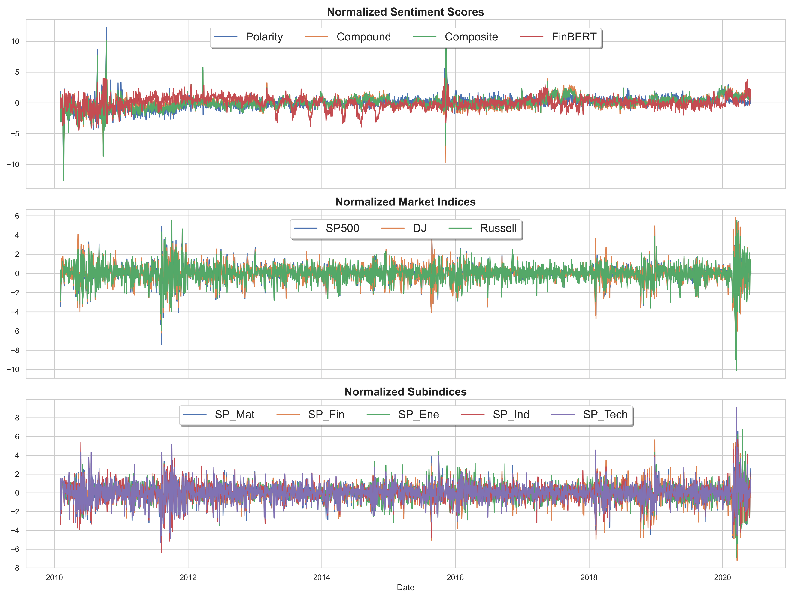
Normalized trends in sentiment scores, broad market indices, and S&P 500 sectoral subindices are shown in Figure A2. Sentiment scores exhibit episodic shifts, with sharp deteriorations during major market stress periods, including the 2011–2012 sovereign debt crisis, the 2015–2016 global growth slowdown, and the COVID-19 shock in early 2020. These sentiment declines broadly align with sharp drawdowns in major equity indices, suggesting that textual sentiment captures investor reactions during periods of heightened uncertainty. Among market indices, the Russell consistently displays larger fluctuations than the SP500 and DJ, reflecting its greater sensitivity to small-cap and high-beta exposures. Sectoral subindices follow similar directional movements but differ in magnitude. Energy and Financials show deeper drawdowns during downturns, consistent with their cyclical and credit-driven risk profiles. In contrast, Technology and Industrials recover more strongly post-crisis, indicating higher sectoral resilience. However, there are also notable decoupling episodes (for instance, in 2013–2014 and parts of 2018) where asset price volatility increased without corresponding shifts in sentiment. These patterns suggest that sentiment scores, while informative, do not fully account for all drivers of return variation. This is especially true when volatility arises from technical shifts, abrupt policy moves, or events that are weakly expressed in headline tone or underrepresented in textual data.

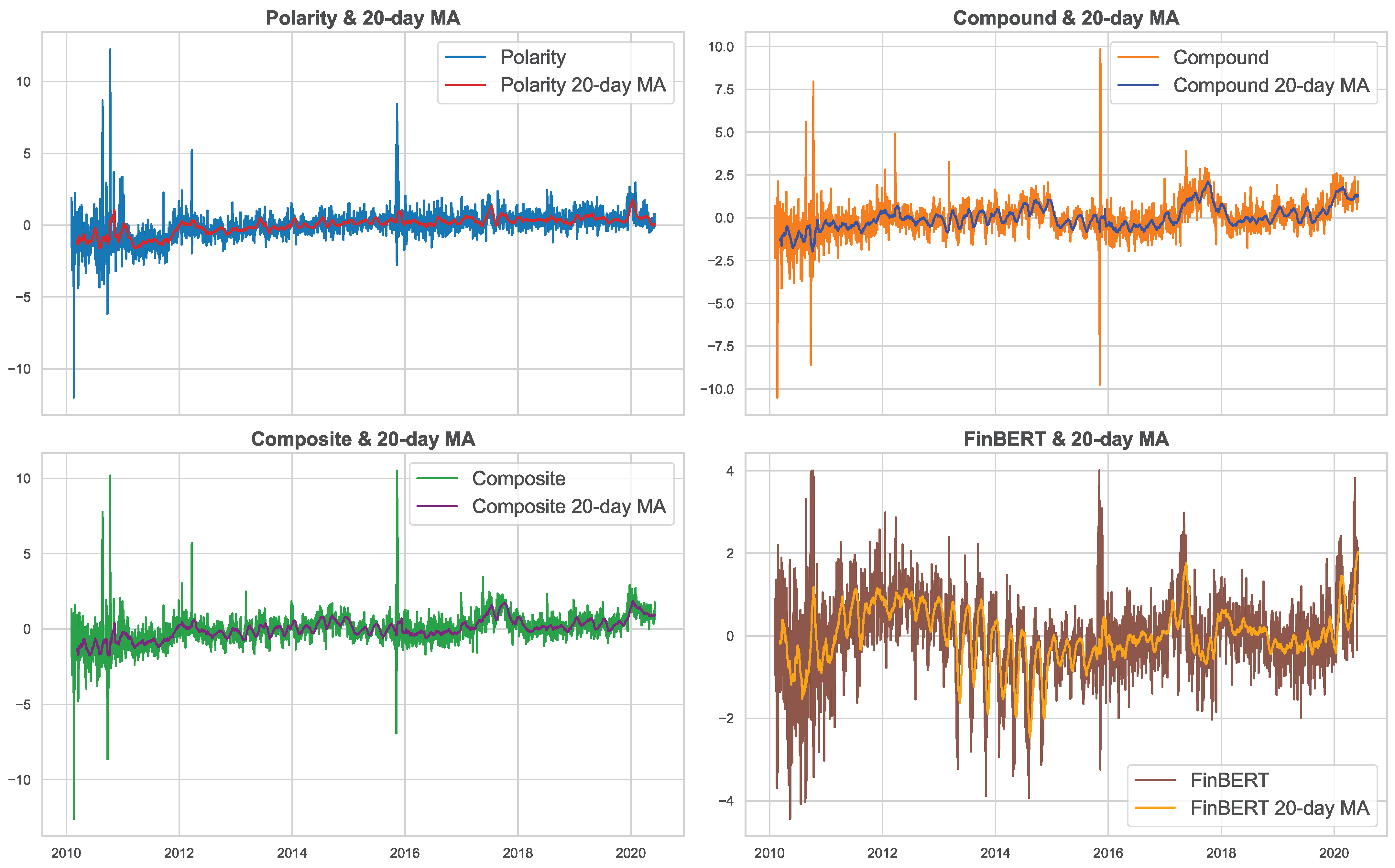
Polarity, Compound, and their Composite sentiment score exhibit broadly aligned trends, marked by noticeable dips during major risk episodes, as shown in Figure 2. These sentiment metrics exhibit smooth cyclical fluctuations, suggesting that they capture gradual changes in sentiment momentum. In contrast, FinBERT displays considerably higher short-term variability and more erratic swings around its moving average. This divergence likely stems from FinBERT’s deeper contextual parsing, which incorporates domain-specific nuances in financial text. Unlike rule-based methods, FinBERT assigns sharper sentiment shifts in response to subtle changes in language, resulting in a higher-frequency signal that is more reactive but also more volatile. Overall, the pronounced spikes in sentiment scores during 2010–2011 correspond to heightened market sensitivity amid pivotal monetary and fiscal developments.

The Federal Reserve’s announcement of QE2 in November 2010 signaled sustained support for economic recovery, fostering optimism. Throughout 2011, Fed communications navigated the tension between accommodative policy and inflationary pressures, further impacting sentiment. Concurrently, the 2011 U.S. debt ceiling crisis and subsequent S&P credit rating downgrade exacerbated uncertainty and risk aversion. The more substantial spike in late 2016 aligns with critical events including the U.S. presidential election, Brexit negotiations, and evolving global trade dynamics, all contributing to elevated market uncertainty and investor sentiment fluctuations.

Sentiment scores also surged markedly in 2020, reflecting the profound macroeconomic disruptions triggered by the COVID-19 pandemic. The rapid escalation of health crises, coupled with extensive fiscal and monetary interventions, heightened market uncertainty and volatility. Compound is notably more responsive to economy-wide shocks, with fluctuations resembling FinBERT, while Polarity remains comparatively muted. The differences between Polarity (TextBlob) and Compound (VADER) arise from their distinct methodologies. VADER’s valence-aware design captures more nuanced and intense sentiment, especially in emotionally charged or informal language. In contrast, TextBlob applies a simpler, rule-based approach that produces more tempered scores. These differences underscore the tools’ complementary strengths and raise the following key question: do such methodological divergences enhance predictive power, or do they merely reflect alternative sentiment constructions?

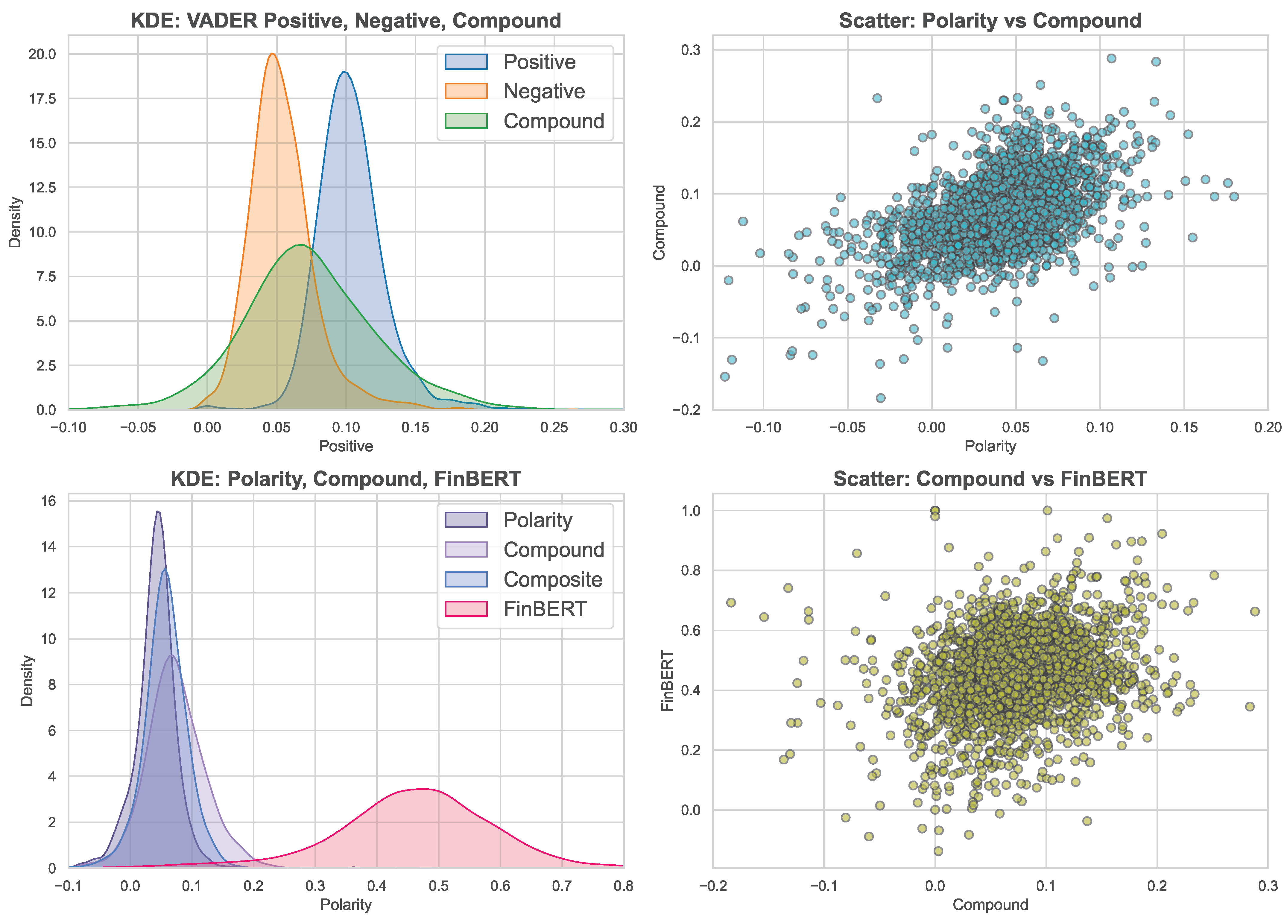
We further explore the relationship between alternative sentiment metrics, and their distributional features, as presented in Figure 3. The first plot, comparing Polarity and Compound, shows a moderately positive but nonlinear association, with higher Polarity scores generally aligning with stronger Compound values. However, the spread suggests that the two metrics are not interchangeable, likely due to their differing sentiment extraction methodologies. The second scatterplot, comparing Compound and FinBERT, shows a broader and more dispersed pattern, indicating weaker alignment. FinBERT values remain concentrated in a narrow range despite wider variation in Compound, reflecting FinBERT’s distinct calibration and contextual sensitivity. These visual patterns highlight methodological divergence across sentiment tools and imply that aggregation or ensemble use of scores may enhance robustness.

The KDE plots in Figure 3 provide smooth estimates of sentiment score distributions across models. The VADER density shows a bimodal shape. One peak near zero corresponds to frequent neutral to mildly negative sentiment. Another peak around 0.10–0.15 indicates moderate positive sentiment. The compound score has a broader, flatter distribution centered near zero with a slight positive skew. This pattern highlights mixed sentiment in financial narratives, typically balanced or mildly optimistic but occasionally marked by extremes. Comparing all sentiment scores, VADER-centric measures cluster tightly around zero with little skew. This points to a conservative sentiment response. In contrast, FinBERT exhibits a sharper, right-skewed distribution; so it detects stronger positive sentiment more frequently. Polarity and Compound scores appear more symmetric and bounded, whereas the Composite score closely mirrors their combined behavior. These differences reflect methodological variation and thereby support the complementarity of these models in capturing nuanced market sentiment.

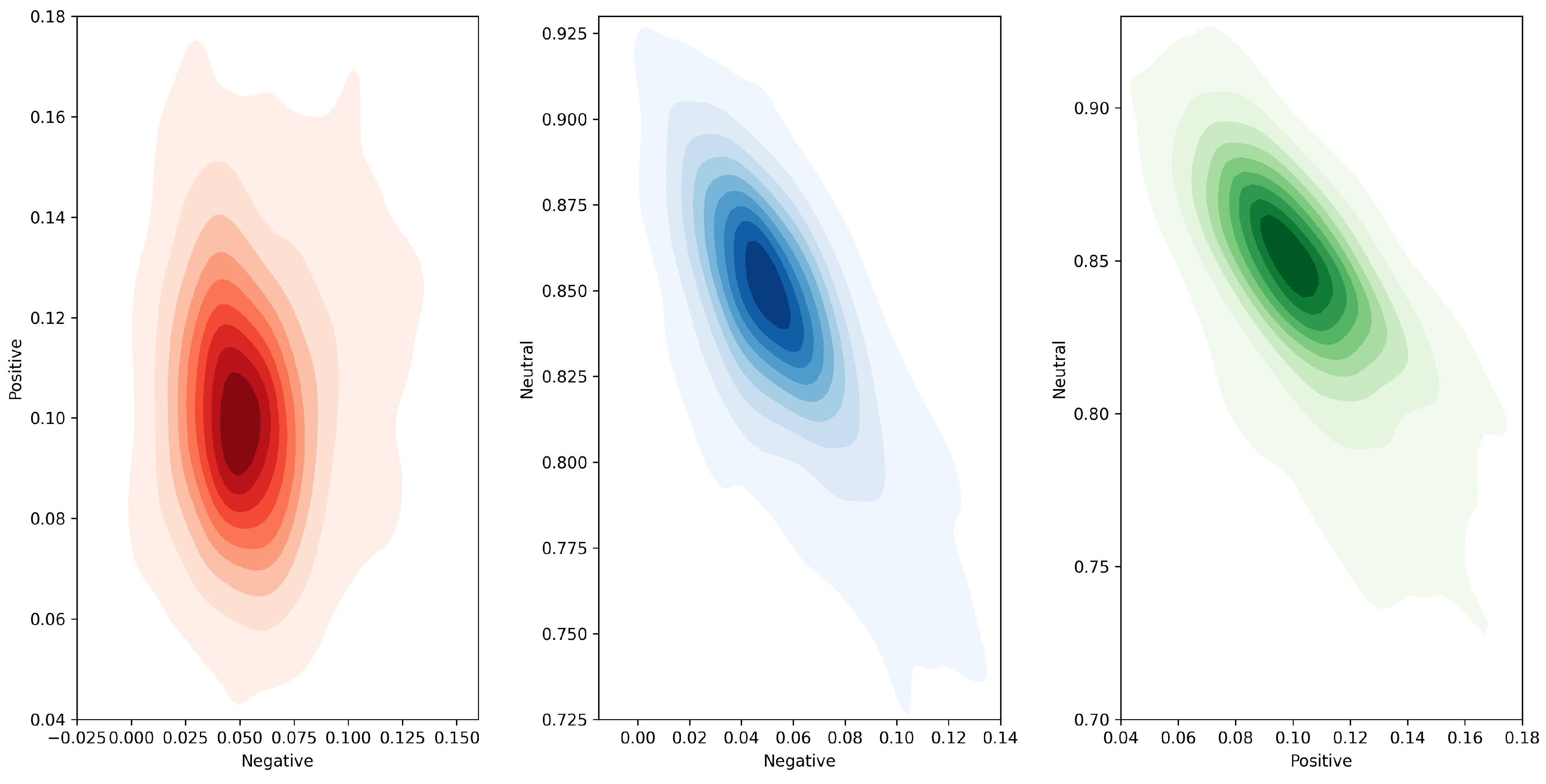
The contour plots of VADER sentiment components (see Figure A3) depict their joint distributions and densities within stock market news. The Positive versus Negative sentiment plot shows a concentrated elliptical distribution centered near a Positive score of 0.08–0.12 and a Negative score of 0.00–0.02. The highest density region indicates most observations have moderate positive sentiment with minimal negativity, reflecting an overall optimistic tone. The Neutral versus Negative plot reveals a dense cluster around Neutral values of 0.82–0.85 and Negative values near 0.00–0.02. This pattern highlights the dominance of neutral sentiment alongside low negative sentiment, suggesting largely balanced or factual narratives. The Neutral versus Positive plot also centers near Neutral 0.82–0.85 and Positive 0.08–0.12. This confirms frequent coexistence of neutral and moderate positive sentiments. Collectively, these plots illustrate VADER’s ability to capture a sentiment landscape dominated by neutral and positive tones, with negative sentiment largely marginal.

A complimentary set of contour plots (see Figure A4) illustrates the joint distributions of TextBlob sentiment scores. The left plot shows Polarity versus Subjectivity with an elliptical concentration near Polarity 0.025–0.050 and Subjectivity 0.175–0.200. The highest density indicates most observations combine slightly positive sentiment with moderate subjectivity, suggesting a balanced but mildly emotional narrative. The right plot depicts Polarity against Objectivity, clustered around Polarity 0.025–0.050 and Objectivity 0.80–0.825. This reflects a predominance of slightly positive sentiment accompanied by high objectivity, indicative of a largely factual yet subtly optimistic tone. Together, these plots reveal TextBlob’s tendency to characterize sentiment with neutral to positive polarity, low subjectivity, and strong objectivity.

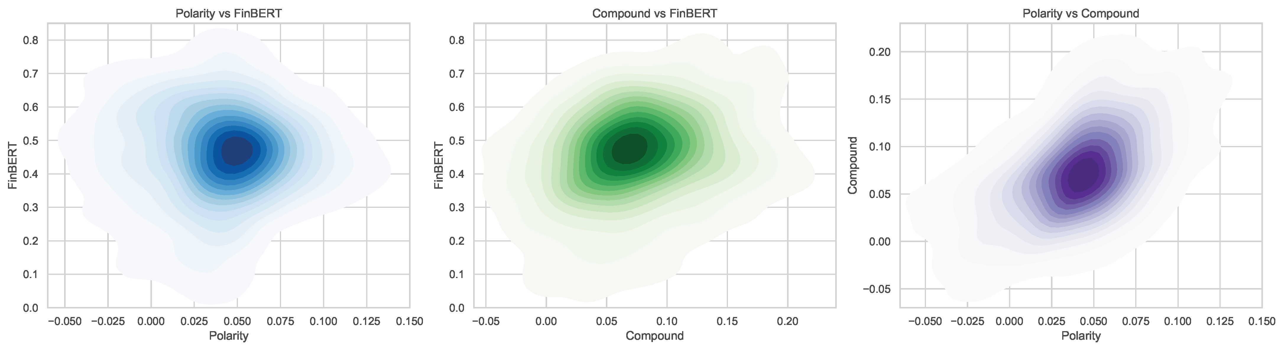
The joint distributions of key sentiment metrics across models are presented in Figure 4. The Polarity versus FinBERT plot reveals a concentrated elliptical distribution spanning Polarity values from approximately 0.00 to 0.15 and FinBERT scores from 0.2 to 0.8. The highest density is centered near moderate Polarity (0.05–0.10) and mid-to-high FinBERT values (0.4–0.6), indicating that moderate positive polarity often coincides with substantial FinBERT sentiment scores.

The Compound versus FinBERT plot shows a similar elliptical pattern, with densities peaking around Compound scores of 0.05–0.15 and FinBERT values between 0.3 and 0.7. This reflects a positive but dispersed association, suggesting that although both metrics capture overlapping sentiment signals, FinBERT exhibits a broader dynamic range. The Polarity versus Compound plot exhibits a moderately strong positive correlation, with a Pearson coefficient of approximately 0.54. This indicates substantial but not perfect alignment between these two sentiment metrics, reflecting differences in their methodologies and sensitivity. The clustering along the diagonal suggests consistent directional agreement, yet the moderate correlation signals that each captures unique sentiment nuances. Lastly, the wider spread in comparisons involving FinBERT underscores its distinct modeling approach and sensitivity to context.

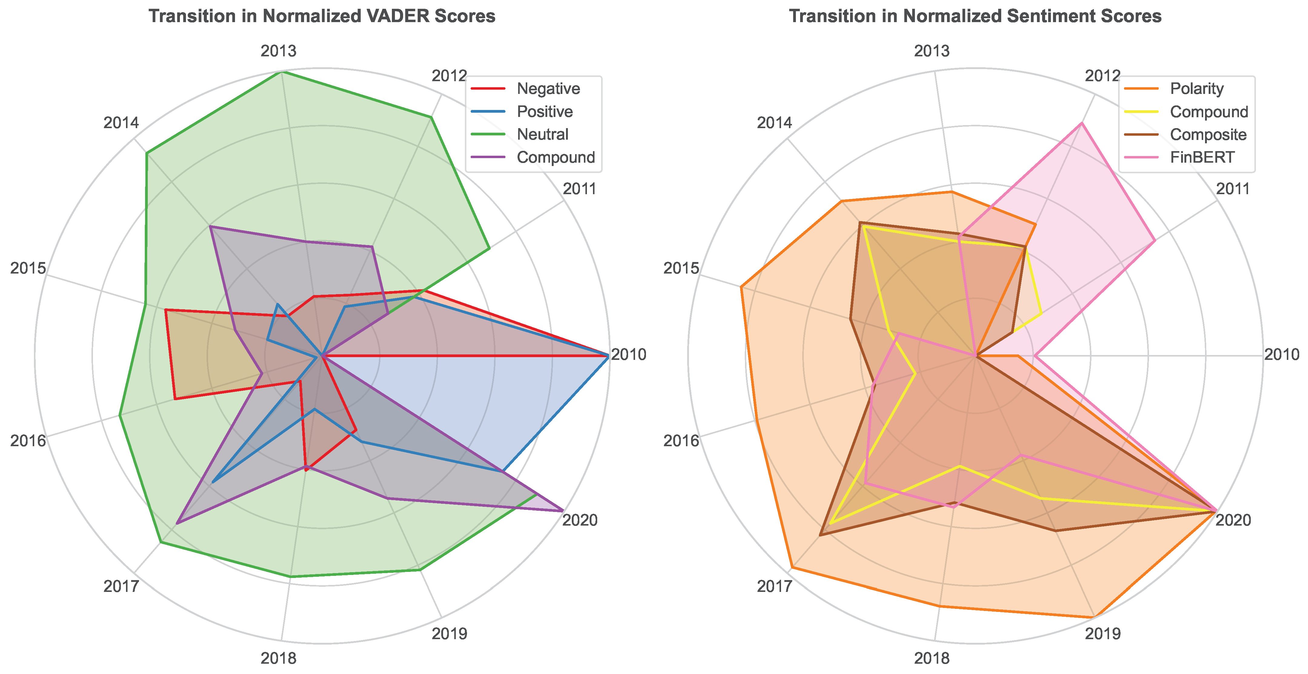
Finally, it is also interesting to look at the temporal evolution of the average annual stock market sentiment over the observed period (see Figure 5). The first radar chart (left) illustrates the annual transitions in normalized VADER sentiment subscores (2010–2020). Over this period, Neutral sentiment consistently dominates, indicating that financial news generally maintains a balanced tone with limited emotional extremes. Positive sentiment maintains a steady presence but shows marked fluctuations, including a subtle decline during the 2011–2012 stress period and a pronounced spike in 2020 driven by optimistic market trends.

Negative sentiment peaks notably in 2010 and 2016–2017, reflecting periods of heightened pessimism aligned with adverse economic conditions. The Compound score shows moderate variation and trends toward neutrality, as it balances market optimism and pessimism. Peaks in 2014, 2017, and 2020 correspond primarily to increases in neutral and mildly positive sentiment and mark episodic shifts in market mood.

The second radar chart (right) depicts annual normalized trends for Polarity, Compound, Composite, and FinBERT scores over the decade. Polarity and Composite scores follow similar trajectories, with incremental shifts in sentiment tone and generally moderate values. Compound scores present a comparable but somewhat more volatile pattern, due to the combination of positive and negative elements. FinBERT differs with more pronounced fluctuations, particularly during stress periods like 2011–2012 and 2020. This indicates greater contextual sensitivity and finer granularity in capturing nuanced sentiment changes. Together, these measures reveal a complex sentiment landscape, where models emphasize distinct facets of market mood. This finding supports the earlier argument on the essential role of multi-dimensional sentiment analysis for capturing financial market emotions accurately.

4.2. Event-Driven Sentiment Dynamics

This section summarizes key sentiment trends occurring on and around (typically $\pm 3$ days) major event-driven news over the period from February 2010 to June 2020, based upon day-centered summary statistics. The sentiment scores around FOMC release dates (day 0) show clear dynamics within a $\pm 3$ day window. FinBERT scores start relatively high at day $-3$ with a mean near 0.49. They gradually decline through the event day and following days, reaching a minimum on day 1 (mean $\approx 0.42$). Scores recover on days 2 and 3, with a marked spike at day 3 (mean $\approx 0.58$). This may reflect delayed market reactions. Polarity scores remain low and fairly stable, fluctuating between approximately 0.05 and 0.04 until day 3. At day 3, there is a pronounced drop to negative values, suggesting transient negative sentiment post-event. Compound scores show moderate variation, declining slightly from day $-3$ to day 1, then recovering. However, by day 3, they shift into negative territory, possibly indicating market uncertainty or mixed interpretations. These patterns imply that sentiment responds to FOMC announcements with initial caution. The tone partially reverses in subsequent days, while late reactions or volatility may drive sharper sentiment swings beyond the event window.

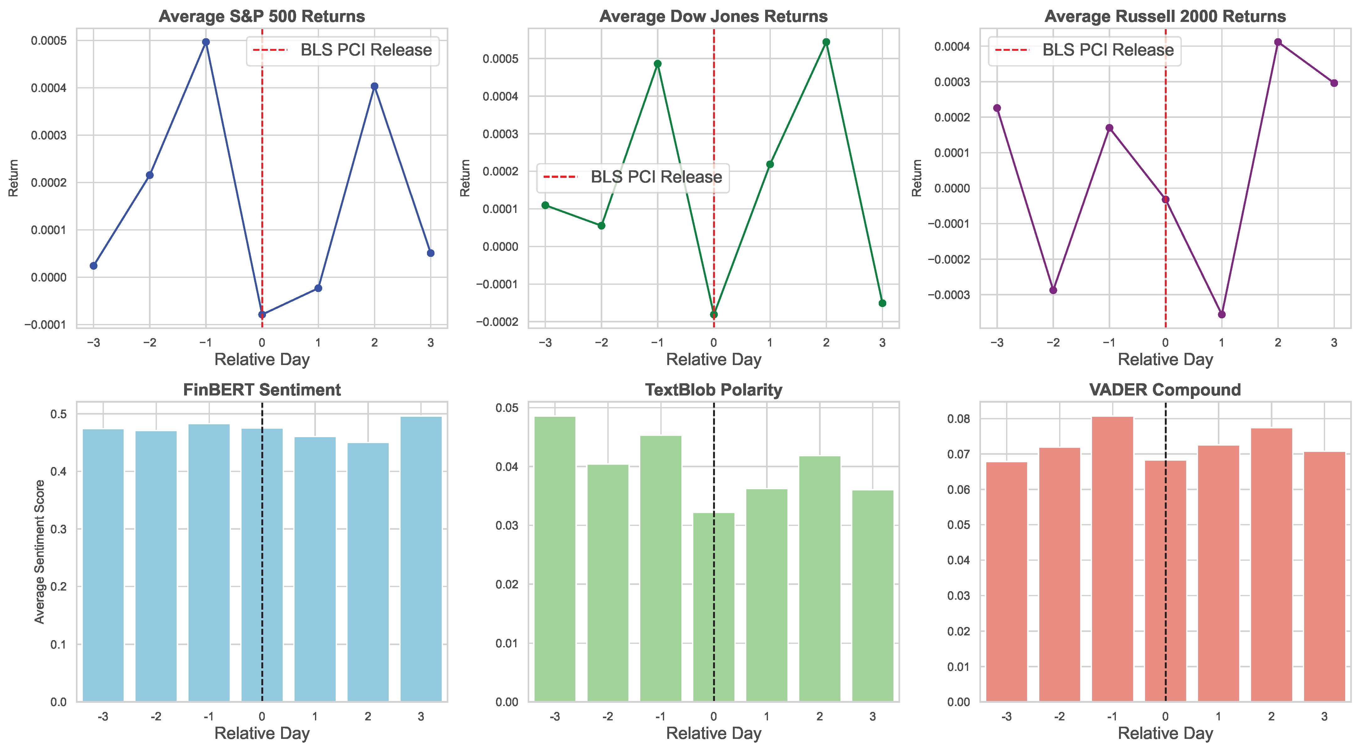
The sentiment scores around BLS PCI release dates (day 0) exhibit relatively stable dynamics within the $\pm 3$ day window. FinBERT scores fluctuate moderately, beginning near 0.47 at day $-3$, peaking at day $-1$ around 0.48, and dipping slightly around the event day and following days, with a recovery to approximately 0.50 by day 3. Polarity scores remain low throughout, generally ranging between 0.03 and 0.05, with a slight dip on the event day to about 0.03, suggesting limited shifts in overt sentiment polarity. Compound scores display moderate variation, peaking slightly before the release at 0.08 and decreasing slightly at day 0, then stabilizing around 0.07 thereafter. Overall, these patterns suggest that sentiment responses to BLS PCI news releases are subtle and mostly balanced. Comparatively, FinBERT captures slightly more nuanced fluctuations compared to Polarity and Compound scores. Its ability to interpret financial jargon and complex sentence structures likely contributes to capturing these finer variations in market sentiment.

The sentiment scores surrounding BLS Employment Situation release dates (day 0) show moderate stability within the $\pm 3$ day window. FinBERT scores start near 0.46 at day $-3$, gradually decline to about 0.44 at day $-1$, then rise slightly on the event day to approximately 0.46. Scores dip sharply on days 1 and 2, though sample sizes there are limited, and recover by day 3 to 0.46. Polarity remains low and relatively stable, fluctuating around 0.04–0.05, with no major deviations on event days. Compound scores vary modestly, peaking at 0.075 just before the event and decreasing slightly on day 0, before rising again by day 3. Similar to the BLS PCI release analysis, these patterns indicate a generally balanced sentiment response to employment news. Nevertheless, FinBERT appears more effective at detecting subtle fluctuations absent in Polarity and Compound scores.

We can also connect the fluctuations in sentiment scores with those of major market indices around these events, as presented in Figure 6, Figure 7 and Figure 8. The FinBERT sentiment score exhibits a distinct U-shaped pattern around FOMC announcements (see Figure 6), decreasing gradually from three days before to the event day, followed by a sharp recovery in the subsequent days. In contrast, both TextBlob Polarity and VADER Compound scores display a subtle W-shaped trajectory, with mild rises and falls prior to the event and a pronounced decline on the third day after the announcement. Regarding market returns, all three indices experience a sharp increase in the days leading up to the announcement. This is followed by a marked decline immediately after the event. Subsequently, the S&P 500 and Dow Jones recover rapidly, whereas the Russell 2000 shows a more volatile pattern with an initial rebound followed by a renewed decline. These dynamics reflect the evolving investor sentiment and market uncertainty around monetary policy releases, highlighting heterogeneous responses across sentiment models and market segments.

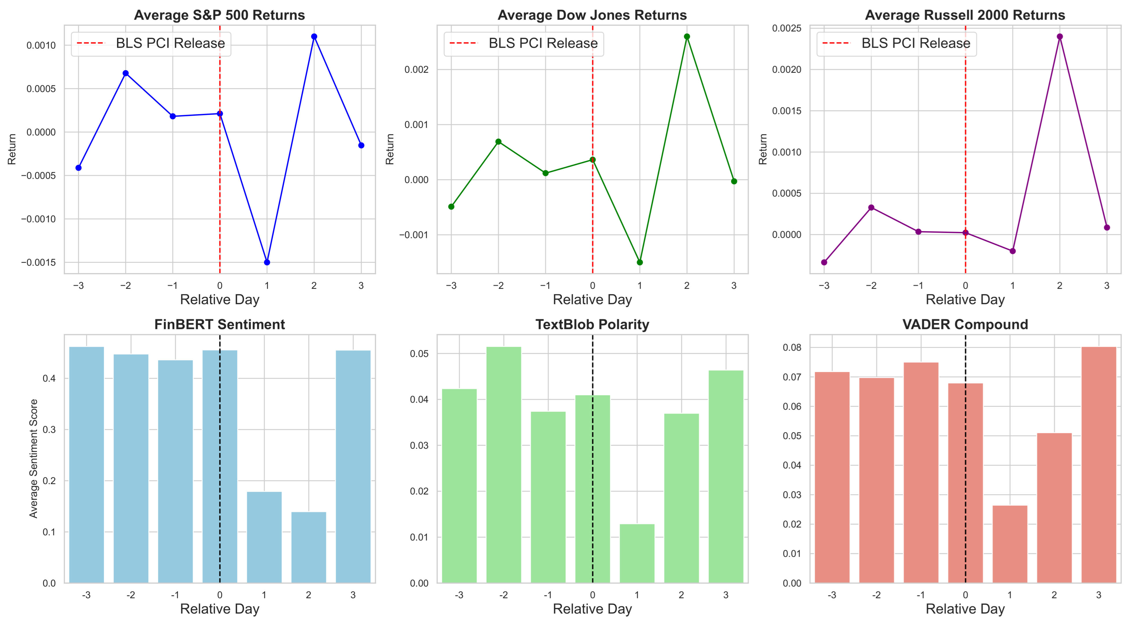
Sentiment and returns exhibit markedly different patterns around the BLS PCI release date (see Figure 7). FinBERT sentiment remains relatively stable with a slight upward trend, while other sentiment metrics reach their lowest average values on the release day, followed by a volatile recovery. The S&P 500 returns increase significantly up to one day before the announcement, then decline sharply on day 0, before mounting a strong rebound in subsequent days. In contrast, the Dow Jones shows a fragile pre-announcement trend and a sharp drop on the release day, while the Russell 2000 experiences an extended decline on day 1. Both indices display erratic, day-specific recovery patterns thereafter. Accordingly, event-driven impacts vary across market segments and call for careful consideration of index-specific dynamics in event studies.

The sentiment response and corresponding stock market adjustment around the BLS Employment Situation release exhibit distinctive dynamics (see Figure 8). FinBERT sentiment shows relative stability in the days leading up to the release.

Following the announcement, it experiences a marked two-day decline before rebounding sharply, a pattern mirrored across all sentiment metrics. The other two sentiment scores display a similar pattern, with recovery commencing on the second day after the release. Market returns mirror these trends, differing mainly in the magnitude of changes across indices. The release day triggers a sharp decline in the S&P 500 and Dow Jones, and a more modest drop in the Russell 2000, followed by a pronounced rebound that reverses on the third day post-announcement. These findings highlight the temporal complexity of sentiment and market reactions. They underscore the importance of capturing both immediate and lagged effects in event studies.

Overall, the analysis of sentiment scores and market returns around FOMC, BLS PCI, and BLS Employment releases reveals distinct yet interrelated dynamics. FinBERT sentiment consistently captures more persistent and smoother shifts. This is shown by its U-shaped decline and rebound around FOMC announcements and steady increase near BLS PCI. These patterns contrast with more volatile, short-term fluctuations detected by lexicon-based metrics like TextBlob and VADER. Lexicon scores exhibit pronounced drops on release days, especially for BLS PCI, indicating sensitivity to immediate event-driven noise. FinBERT moderates this through contextual understanding. Market returns reflect heterogeneous responses. Pre-announcement rallies followed by sharp declines on release days are common. Subsequent rebounds vary by index. The Russell 2000 shows greater volatility and delayed recoveries compared to the S&P 500 and Dow Jones. This highlights size- and sector-specific sensitivities.

4.3. Supervised Learning Outcomes: Classification Task

As a preliminary step preceding the classification tasks, we conducted tests for serial autocorrelation and stationarity on the market-state-centered binary target variables. The results, summarized in

Table A4. Serial autocorrelation (Ljung–Box) and stationarity (ADF) test results.

Variable	Ljung–Box Test (lag 10)		ADF Test
	Statistic	p-Value	Statistic	p-Value
SP500_Binary	6.8413	0.7403	−52.4071	<0.0001
DJ_Binary	8.8734	0.5442	−51.7241	<0.0001
Russell_Binary	4.3019	0.9327	−51.9556	<0.0001
SP_Materials_Binary	7.2402	0.7026	−51.4985	<0.0001
SP_Financial_Binary	7.9604	0.6327	−52.5443	<0.0001
SP_Energy_Binary	12.6267	0.2453	−16.2423	<0.0001
SP_Industrial_Binary	11.1941	0.3426	−54.5405	<0.0001
SP_Tech_Binary	9.2226	0.5111	−51.1890	<0.0001

, show that the Ljung–Box test fails to reject the null hypothesis, indicating no significant autocorrelation up to lag 10. Concurrently, the Augmented Dickey-Fuller (ADF) test rejects the null hypothesis of a unit root, confirming that these binary series are stationary. The classification performance using the one-factor model with VADER Compound Score as the sole feature shows moderate predictive power (see

Table A5. Classification performance (one-factor model, feature: VADER compound score).

Model	Class	S&P 500		DJ		Russell
		F1	Accur.	F1	Accur.	F1	Accur.
XGBoost	Class 0	0.49	0.51	0.50	0.51	0.49	0.52
	Class 1	0.55		0.56		0.55
AdaBoost	Class 0	0.54	0.52	0.53	0.52	0.51	0.48
	Class 1	0.61		0.60		0.57
Bagging	Class 0	0.51	0.52	0.53	0.55	0.50	0.51
	Class 1	0.54		0.57		0.53
RandomForest	Class 0	0.51	0.52	0.53	0.55	0.50	0.52
	Class 1	0.54		0.58		0.53
GBM	Class 0	0.55	0.53	0.55	0.54	0.55	0.53
	Class 1	0.62		0.62		0.62
Stacking	Class 0	0.57	0.52	0.59	0.51	0.58	0.50
	Class 1	0.64		0.66		0.65

Note: Class 0: Bearish Market ($returns<0$), and Class 1: Bullish Market ($returns>0$).

). The F1 scores for Class 1 (Bullish Market) consistently outperform those for Class 0 (bearish market) across all methods, indicating a relative ease in predicting positive return days. Accuracy values remain close to the 50–53% range, reflecting the challenging nature of the binary market direction prediction task with only a sentiment feature. Notably, ensemble methods such as Stacking and GBM outperform simpler methods like AdaBoost and Bagging, yielding higher F1 scores and slightly better accuracy, particularly for bullish market days. The Russell index generally shows marginally higher accuracy and F1 values, potentially reflecting more discernible sentiment patterns in that index relative to the others.

When replacing VADER with FinBERT sentiment score, classification results improve notably, especially for Class 1 (see

Table A6. Classification performance (one-factor model, feature: FinBERT sentiment score).

Model	Class	S&P 500		DJ		Russell
		F1	Accuracy	F1	Accuracy	F1	Accuracy
XGBoost	Class 0	0.49	0.53	0.50	0.52	0.51	0.51
	Class 1	0.55		0.57		0.58
AdaBoost	Class 0	0.54	0.52	0.56	0.51	0.57	0.50
	Class 1	0.61		0.63		0.64
Bagging	Class 0	0.51	0.52	0.49	0.51	0.50	0.50
	Class 1	0.52		0.52		0.50
RandomForest	Class 0	0.52	0.52	0.50	0.51	0.50	0.50
	Class 1	0.52		0.53		0.50
GBM	Class 0	0.54	0.51	0.55	0.51	0.56	0.52
	Class 1	0.61		0.62		0.63
Stacking	Class 0	0.59	0.49	0.60	0.50	0.59	0.50
	Class 1	0.66		0.67		0.66

Note: Class 0: bearish market ($\mathrm{returns}<0$), and Class 1: bullish market ($\mathrm{returns}>0$).

). F1 scores for bullish market predictions increase consistently across all models and indices, with Stacking and AdaBoost again providing the highest performance. Accuracy is also slightly enhanced, ranging mostly between 49% and 53%. The difference between F1 scores of bullish and bearish classes is narrower here compared to the VADER-based model, suggesting FinBERT’s sentiment captures more balanced signals across market directions. Interestingly, the S&P 500 shows a slight uptick in accuracy compared to VADER, implying FinBERT’s domain-specific NLP capabilities better align with financial text nuances relevant to the broader market. The DJ and Russell indices maintain similar improvements, underscoring FinBERT’s robustness in capturing sentiment features.

Comparatively speaking, FinBERT sentiment features improve classification performance notably compared to VADER’s compound scores, raising accuracy on average by approximately 1.5 to 2 percentage points. Additionally, FinBERT improves bullish class F1 scores by approximately 2 to 7 percentage points, depending on the model and asset. It also reduces the imbalance between bullish and bearish class F1 scores by about 2 to 5 percentage points. Ensemble methods like Stacking and GBM achieve the highest gains in both sentiment feature sets, but their improvements with FinBERT are more pronounced (3–5 percentage points higher in F1 scores). Accuracy values generally hover around 50–53%, which is only slightly better than the 50% baseline expected from random classification in a balanced binary setting. Sentiment alone does not fully explain the complexity of market movements, so the models struggle to achieve high predictive power.

The one-factor model leveraging VADER compound scores as the predictor demonstrates limited but measurable classification ability across the S&P 500 sector subindices (see

Table A7. Classification performance (one-factor model, feature: VADER compound score).

Model	Class	Materials		Financial		Energy		Industrials		Tech
		F1	Accur.	F1	Accur.	F1	Accur.	F1	Accur.	F1	Accur.
XGBoost	Class 0	0.52	0.52	0.50	0.50	0.49	0.52	0.47	0.51	0.45	0.47
	Class 1	0.59		0.57		0.55		0.54		0.52
AdaBoost	Class 0	0.51	0.50	0.56	0.51	0.50	0.53	0.51	0.52	0.53	0.49
	Class 1	0.58		0.63		0.56		0.58		0.58
Bagging	Class 0	0.51	0.52	0.49	0.53	0.49	0.51	0.50	0.51	0.48	0.51
	Class 1	0.54		0.55		0.53		0.52		0.53
RandomForest	Class 0	0.52	0.52	0.50	0.53	0.49	0.51	0.51	0.52	0.49	0.51
	Class 1	0.54		0.56		0.53		0.52		0.53
GBM	Class 0	0.54	0.50	0.55	0.51	0.48	0.48	0.50	0.52	0.51	0.46
	Class 1	0.60		0.62		0.54		0.58		0.55
Stacking	Class 0	0.59	0.51	0.59	0.51	0.50	0.52	0.54	0.50	0.58	0.50
	Class 1	0.66		0.66		0.56		0.61		0.64

Note: Class 0: bearish market ($returns<0$), and Class 1: bullish market ($returns>0$). S&P 500 subindices: Materials, Financial, Energy, Industrials, and Technology.

). For all sectors and methods, F1 scores for the bullish market class surpass those of the bearish class, suggesting that upward market movements are relatively easier to predict from VADER sentiment alone. Accuracy scores hover around 50–52%, marginally exceeding random classification, reflecting the difficulty of relying solely on a single sentiment feature. Among the algorithms tested, ensemble approaches such as Stacking and GBM consistently deliver superior results, especially for positive return days. Notably, Materials and Financial sectors tend to yield slightly better results, while Technology lags behind, possibly due to more complex or less directly sentiment-driven price behaviors.

Substituting VADER with FinBERT sentiment scores yields clearer gains in predictive performance across all sectors and classifiers (see

Table A8. Classification performance (one-factor model, feature: FinBERT sentiment score).

Model	Class	Materials		Financial		Energy		Industrials		Tech
		F1	Accur.	F1	Accur.	F1	Accur.	F1	Accur.	F1	Accur.
XGBoost	Class 0	0.46	0.52	0.55	0.54	0.44	0.48	0.49	0.51	0.45	0.50
	Class 1	0.53		0.62		0.49		0.56		0.52
AdaBoost	Class 0	0.54	0.47	0.59	0.50	0.55	0.50	0.54	0.50	0.53	0.52
	Class 1	0.61		0.66		0.61		0.61		0.60
Bagging	Class 0	0.47	0.47	0.49	0.53	0.44	0.49	0.43	0.46	0.44	0.51
	Class 1	0.47		0.56		0.49		0.43		0.51
RandomForest	Class 0	0.47	0.47	0.49	0.53	0.46	0.49	0.43	0.45	0.44	0.51
	Class 1	0.47		0.56		0.49		0.43		0.50
GBM	Class 0	0.52	0.46	0.56	0.51	0.51	0.49	0.50	0.48	0.52	0.49
	Class 1	0.59		0.63		0.58		0.56		0.59
Stacking	Class 0	0.59	0.49	0.58	0.52	0.56	0.49	0.57	0.49	0.58	0.52
	Class 1	0.66		0.64		0.63		0.64		0.65

Note: Class 0: bearish market ($returns<0$), and Class 1: bullish market ($returns>0$). S&P 500 subindices: Materials, Financial, Energy, Industrials, and Technology.

). The improvements are most marked in the F1 scores for bullish market days, which rise steadily for all models. Stacking and AdaBoost continue to lead in performance, while accuracy metrics, although still moderate (approximately 49–54%), slightly improve in sectors such as Financials and Industrials, indicating FinBERT’s enhanced ability to capture sector-specific sentiment signals. Furthermore, the gap between bullish and bearish class F1 scores narrows, signifying a more balanced prediction capability across classes when using FinBERT, with notable increases in bearish class performance for Energy and Industrials sectors.

In summary, FinBERT-based sentiment consistently enhances classification effectiveness compared to VADER across S&P 500 subindices. Bullish class F1 scores increase by roughly 3 to 7 percentage points depending on the sector and model, while the imbalance between class performances decreases by about 2 to 6 points, indicating a more equitable model output. Ensemble methods again provide the best predictive power, and their advantage is more prominent when paired with FinBERT features. However, overall accuracy remains close to the random baseline, underscoring the challenge of predicting market direction with single-factor sentiment models. These findings emphasize the need for more comprehensive feature sets to capture the multifaceted drivers of market movements.

In the light of our previous findings, we explore the predictive accuracy based on the FinBERT unrestricted model (see

Table 2. Classification report (FinBERT; unrestricted model, rounded to two decimals).

Model	S&P 500			Dow Jones			Russell			S&P Materials
	F1 (0)	F1 (1)	Acc	F1 (0)	F1 (1)	Acc	F1 (0)	F1 (1)	Acc	F1 (0)	F1 (1)	Acc
XGB	0.66	0.67	0.66	0.62	0.64	0.63	0.63	0.64	0.64	0.65	0.65	0.65
AdaB	0.70	0.71	0.70	0.65	0.67	0.66	0.66	0.72	0.69	0.67	0.70	0.69
Bagg.	0.64	0.66	0.65	0.63	0.66	0.65	0.65	0.66	0.66	0.65	0.65	0.65
RF	0.68	0.69	0.68	0.63	0.66	0.65	0.66	0.66	0.66	0.66	0.67	0.66
GBM	0.68	0.69	0.69	0.65	0.68	0.67	0.66	0.69	0.68	0.68	0.69	0.69
Stack.	0.68	0.70	0.69	0.65	0.69	0.67	0.66	0.69	0.67	0.68	0.70	0.69
Model	S&P Financial			S&P Energy			S&P Industrials			S&P Tech
	F1 (0)	F1 (1)	Acc	F1 (0)	F1 (1)	Acc	F1 (0)	F1 (1)	Acc	F1 (0)	F1 (1)	Acc
XGB	0.65	0.68	0.67	0.59	0.58	0.58	0.63	0.62	0.62	0.63	0.64	0.64
AdaB	0.70	0.71	0.70	0.64	0.65	0.64	0.65	0.67	0.66	0.67	0.69	0.68
Bagg.	0.67	0.71	0.69	0.62	0.61	0.61	0.64	0.63	0.64	0.64	0.63	0.64
RF	0.67	0.71	0.69	0.63	0.62	0.62	0.65	0.62	0.64	0.62	0.62	0.62
GBM	0.68	0.71	0.70	0.63	0.63	0.63	0.68	0.66	0.67	0.67	0.68	0.67
Stacking	0.70	0.74	0.72	0.63	0.62	0.63	0.68	0.67	0.67	0.65	0.66	0.66

). This classification report reveals consistently strong performance across all major market indices and subindices. Specifically, F1 scores generally range from the mid-0.60 s to low 0.70 s and accuracy levels consistently around 62 to 72 percentage points. Ensemble methods like Stacking and GBM outperform individual models such as XGBoost and Random Forest. This shows that combining predictions helps capture complex relationships among VIX, volume, Treasury yield, and FinBERT sentiment. The bullish market class (Class 1) has slightly higher F1 scores than the bearish class (Class 0), indicating the model detects positive returns more effectively. This aligns with earlier findings that bullish signals are often more identifiable.

Performance across sector subindices is fairly consistent, with minor differences likely due to sector-specific sentiment strength and market behavior. Balanced accuracy values above 60% demonstrate predictive power well beyond random chance. The average gap in F1 scores between the bullish (Class 1) and bearish (Class 0) classes across models and assets is roughly 3 to 4 percentage points. This indicates a moderate imbalance, where the model predicts bullish market days somewhat better than bearish ones.

Comparing the FinBERT-based unrestricted model to the VADER-based model (see

Table A9. Classification report (VADER; unrestricted model, rounded to two decimals).

Model	S&P 500			Dow Jones			Russell			S&P Materials
	F1 (0)	F1 (1)	Acc	F1 (0)	F1 (1)	Acc	F1 (0)	F1 (1)	Acc	F1 (0)	F1 (1)	Acc
XGB	0.65	0.67	0.66	0.60	0.64	0.62	0.62	0.65	0.64	0.67	0.69	0.68
AdaB	0.68	0.70	0.69	0.65	0.68	0.66	0.64	0.70	0.67	0.70	0.71	0.70
Bagg.	0.68	0.69	0.69	0.64	0.67	0.66	0.62	0.65	0.64	0.65	0.65	0.65
RF	0.69	0.71	0.70	0.64	0.68	0.66	0.64	0.66	0.65	0.68	0.68	0.68
GBM	0.69	0.70	0.70	0.65	0.69	0.67	0.65	0.70	0.68	0.68	0.70	0.69
Stacking	0.69	0.70	0.70	0.64	0.68	0.66	0.65	0.70	0.68	0.68	0.71	0.70
Model	S&P Financial			S&P Energy			S&P Industrials			S&P Tech
	F1 (0)	F1 (1)	Acc	F1 (0)	F1 (1)	Acc	F1 (0)	F1 (1)	Acc	F1 (0)	F1 (1)	Acc
XGB	0.67	0.71	0.69	0.61	0.63	0.62	0.64	0.64	0.64	0.62	0.64	0.63
AdaB	0.73	0.74	0.73	0.63	0.65	0.64	0.65	0.67	0.66	0.66	0.70	0.68
Bagg.	0.67	0.71	0.69	0.64	0.62	0.63	0.65	0.64	0.64	0.63	0.64	0.64
RF	0.69	0.74	0.72	0.65	0.64	0.65	0.67	0.66	0.66	0.61	0.63	0.62
GBM	0.70	0.73	0.71	0.65	0.65	0.65	0.66	0.66	0.66	0.68	0.69	0.69
Stacking	0.70	0.73	0.72	0.64	0.64	0.64	0.66	0.65	0.65	0.67	0.68	0.68

) reveals modest yet consistent improvements. FinBERT generally produces higher F1 scores for the bullish market class, exceeding VADER by approximately 1 to 3 percentage points. Balanced accuracy values for both models range between 62% and 72%, indicating solid but not flawless predictive capability. The narrower gap between bullish and bearish F1 scores in the FinBERT model suggests improved balance in classification performance. Sector-level results show stable patterns with minor variations reflecting differences in sentiment strength and market volatility. Both models deliver classification accuracy well above the 50% random baseline, yet neither achieves near-perfect prediction. This highlights the complexity and inherent noise of forecasting financial markets using sentiment as the primary feature.

To explore the marginal contribution of sentiment inthese classification tasks, we have derived the difference in F1 scores and balanced accuracy between unrestricted models (VADER and FinBERT-centered, respectively) and the restricted ones (excluding news sentiment as a feature). The estimated results indicate that the inclusion of VADER sentiment (see

Table A10. Performance differences (VADER; unrestricted vs. restricted model).

Model	S&P 500			Dow Jones			Russell			S&P Materials
	F1 (0)	F1 (1)	Acc	F1 (0)	F1 (1)	Acc	F1 (0)	F1 (1)	Acc	F1 (0)	F1 (1)	Acc
XGB	0.015	0.016	0.016	0.033	0.029	0.031	0.017	0.021	0.019	0.040	0.041	0.041
AdaB	−0.011	0.003	−0.004	−0.010	0.009	0.000	−0.008	−0.010	−0.010	0.021	0.014	0.017
Bagg.	0.038	0.028	0.033	0.059	0.043	0.050	−0.016	0.015	0.000	−0.014	−0.017	−0.016
RF	0.017	0.021	0.019	0.031	0.030	0.031	0.001	0.003	0.002	0.013	−0.005	0.003
GBM	−0.005	0.005	0.000	−0.010	0.005	−0.002	−0.007	−0.008	−0.008	−0.005	0.005	0.000
Stack.	−0.010	0.002	−0.004	−0.015	0.002	−0.006	−0.004	0.007	0.002	−0.003	−0.001	−0.002
Model	S&P Financial			S&P Energy			S&P Industrials			S&P Tech
	F1 (0)	F1 (1)	Acc	F1 (0)	F1 (1)	Acc	F1 (0)	F1 (1)	Acc	F1 (0)	F1 (1)	Acc
XGB	−0.005	0.008	0.001	0.012	0.026	0.020	0.022	0.006	0.013	0.044	0.044	0.044
AdaB	0.008	0.011	0.010	−0.005	−0.014	−0.010	−0.011	0.006	−0.001	0.008	0.011	0.010
Bagg.	−0.016	0.006	−0.005	0.006	−0.010	−0.002	0.009	0.019	0.014	0.034	0.036	0.035
RF	0.016	0.029	0.023	0.004	−0.004	−0.000	0.020	0.026	0.024	−0.009	0.013	0.002
GBM	−0.003	−0.005	−0.004	0.005	0.011	0.008	−0.030	−0.004	−0.016	0.026	0.028	0.027
Stacking	−0.004	−0.000	−0.002	−0.013	−0.010	−0.012	−0.040	−0.025	−0.032	0.009	0.014	0.012

) yields small but generally positive improvements in F1 scores and accuracy across several assets and models, with the most notable gains observed for XGBoost and Random Forest in indices like S&P 500, Dow Jones, and Russell. However, improvements are inconsistent for other methods such as AdaBoost, GBM, and Stacking, where some differences are negative or negligible, particularly across certain sectors like Energy and Industrials. The mixed performance suggests that while VADER sentiment adds some predictive value, its contribution is modest and model-dependent. This underscores the limited incremental power of generic sentiment features in complex market state prediction tasks.

The classification results when sentiment is proxied by FinBERT score (see

Table A11. Performance differences (FinBERT; unrestricted vs. restricted model).

Model

S&P 500

Dow Jones

Russell

S&P Materials

F1 (0)

F1 (1)

Acc

F1 (0)

F1 (1)

Acc

F1 (0)

F1 (1)

Acc

F1 (0)

F1 (1)

Acc

XGB

0.025

0.014

0.019

0.050

0.029

0.039

0.022

0.014

0.017

0.020

−0.001

0.009

AdaB

0.015

0.012

0.013

−0.008

−0.004

−0.006

0.019

0.007

0.011

−0.003

0.002

0.000

Bagg.

−0.004

−0.004

−0.004

0.048

0.034

0.040

0.014

0.024

0.019

−0.013

−0.010

−0.012

RF

0.001

0.006

0.004

0.022

0.013

0.017

0.023

0.005

0.013

−0.007

−0.016

−0.012

GBM

−0.017

−0.003

−0.009

−0.000

0.004

0.002

−0.004

−0.017

−0.012

−0.003

−0.005

−0.004

Stack.

−0.013

−0.003

−0.007

−0.006

0.012

0.004

0.007

−0.009

−0.002

−0.009

−0.006

−0.008

Model

S&P Financial

S&P Energy

S&P Industrials

S&P Tech

F1 (0)

F1 (1)

Acc

F1 (0)

F1 (1)

Acc

F1 (0)

F1 (1)

Acc

F1 (0)

F1 (1)

Acc

XGB

−0.022

−0.017

−0.019

−0.013

−0.030

−0.022

0.011

−0.018

−0.005

0.054

0.047

0.050

AdaB

−0.019

−0.016

−0.018

0.002

−0.013

−0.006

−0.001

0.001

0.000

0.017

−0.001

0.008

Bagg.

−0.007

−0.002

−0.004

−0.012

−0.023

−0.018

0.002

0.010

0.006

0.041

0.025

0.033

RF

−0.012

0.003

−0.004

−0.020

−0.026

−0.023

0.004

−0.013

−0.005

−0.005

−0.002

−0.004

GBM

−0.019

−0.019

−0.019

−0.009

−0.010

−0.010

−0.013

−0.001

−0.007

0.016

0.011

0.014

Stack.

0.003

0.005

0.004

−0.020

−0.026

−0.023

−0.017

−0.009

−0.013

−0.009

−0.006

−0.008

) also reveal mixed effects: certain models like XGBoost show consistent improvements in F1 scores and accuracy across several indices, particularly S&P 500, Dow Jones, and Russell, with gains often between 1 and 5 percentage points. However, other models, including AdaBoost, GBM, and Stacking, exhibit mostly marginal or even negative differences, especially in sectors such as S&P Financial, Energy, and Industrials. These findings suggest that while FinBERT sentiment can enhance market state predictions in some contexts, its benefit is uneven across models and sectors. Comparatively, VADER generally provides more consistent positive improvements across models and sectors, with several gains exceeding 2–4 percentage points in F1 and accuracy metrics. In contrast, FinBERT’s impact is more variable, showing strong improvements mainly for XGBoost but frequent marginal or negative effects for other ensemble methods. Thus, while FinBERT’s domain-specific embeddings offer richer sentiment information, their integration into complex models may require further tuning. We observe consistent results when lagged sentiment scores are included as predictive features.

These findings offer actionable insights for portfolio managers and financial analysts aiming to enhance predictive models. FinBERT-based sentiment improves classification performance, especially for bullish market states, aiding short-term positioning and tactical trades. Ensemble models like GBM and Stacking benefit the most, suggesting that advanced algorithms better capture subtle sentiment patterns. Sector-specific gains, particularly in Financials and Materials sectors, indicate that sentiment tools may be more effective in news-sensitive industries. However, accuracy levels remain modest, and sentiment signals alone do not suffice for reliable forecasting. Thus, analysts should treat sentiment as a complementary input, best used alongside structural indicators like VIX, volume, and interest rates, etc.

4.4. Demystifying Classification Bias

This section initially addresses the classification bias expressed through constantly higher F1 score for Class 1 (Bullish state), despite the application of smoothing and model calibration. A closer look at the one-factor (FinBERT) model (see

Table A12. Average difference in F1 Scores ($F{1}_{\mathrm{Bullish}}-F{1}_{\mathrm{Bearish}}$, FinBERT, one-factor model).

Asset/Model	XGB	AdaB	Bagging	RF	GBM	Stacking	Average
S&P 500	0.06	0.07	0.01	0.00	0.07	0.07	0.04
Dow Jones	0.07	0.07	0.03	0.03	0.07	0.07	0.05
Russell	0.07	0.07	0.00	0.00	0.07	0.07	0.04
Materials	0.07	0.07	0.00	0.00	0.07	0.07	0.05
Financial	0.07	0.07	0.07	0.07	0.07	0.06	0.07
Energy	0.05	0.06	0.05	0.03	0.07	0.09	0.06
Industrials	0.07	0.07	0.09	0.09	0.06	0.07	0.08
Tech	0.07	0.07	0.07	0.06	0.07	0.07	0.07
Average	0.07	0.07	0.04	0.04	0.07	0.07	—

) indicate still consistently higher predictive performance for bullish market days compared to bearish ones, which indicates a clear classification bias. More formally, the models favor identifying bullish market conditions with roughly 6 to 7 percentage points better F1 scores on average. This bias is most pronounced in certain sectoral assets (such as Financials, Industrials, and Tech sectors), where the F1 gap reaches up to 0.09 for certain models like Bagging and RandomForest. Conversely, lower differences in the Russell and Materials indices (around 0.00 to 0.03 for some models) imply more balanced class predictions or perhaps less distinctive sentiment signals for bearish states in those indices.

Across models, AdaBoost, Gradient Boosting Machines (GBM), and Stacking ensembles show the highest average bullish-bearish F1 gaps (≈0.07). This suggests that ensemble methods amplify this bias compared to simpler learners like Bagging and Random Forests (gaps hover near 0.03 to 0.04). This aligns with concerns that ensemble classifiers may overfit to dominant or more frequent market states, potentially reinforcing structural biases in the training data. Therefore, while smoothing and calibration enhance overall model reliability, these steps appear insufficient to fully correct classification imbalance in this one-factor specification. This bias warrants further investigation, ideally through exploration of additional features (the unrestricted model) and corresponding year-by-year analysis of the classification metrics.

In the unrestricted model, the cross-model and cross-class comparisons indicate a substantially reduced gap in F1 scores between bullish and bearish classes (See

Table 3. Average difference in F1 Scores ($F{1}_{\mathrm{Bullish}}-F{1}_{\mathrm{Bearish}}$, FinBERT, unrestricted model).

Asset/Model	XGB	AdaB	Bagg.	RF	GBM	Stack.	Average
S&P 500	0.01	0.00	0.02	0.02	0.02	0.02	0.01
Dow Jones	0.01	0.02	0.02	0.03	0.02	0.02	0.02
Russell	0.01	0.05	0.02	0.01	0.02	0.02	0.02
Materials	0.01	0.04	0.01	0.01	0.01	0.01	0.01
Financial	0.02	0.01	0.01	0.03	0.00	0.00	0.01
Energy	0.01	−0.01	0.00	0.00	0.01	−0.01	0.00
Industrials	0.01	0.02	0.01	0.02	−0.02	−0.01	0.01
Tech	0.01	0.01	0.02	0.00	0.03	0.01	0.01
Average	0.01	0.02	0.01	0.02	0.01	0.01	—

). Unlike the one-factor FinBERT-only model, which exhibited an average class imbalance around 4–7 percentage points, the unrestricted model’s differences cluster close to zero or just 1–2 percentage points on average across assets and models.

Features such as volatility measures (VIX), trading volume, and term structure variables likely provide complementary and stabilizing information that helps the model better distinguish bearish market states. Moreover, these diverse signals may capture structural market dynamics and risk factors that sentiment metrics cannot fully represent on their own. This supports the idea that sentiment alone, while informative, is insufficient for fully balanced classification; therefore, multi-factor models are essential for addressing inherent market asymmetries and noise.

A refined analysis of average annual differences between F1 scores ($F{1}_{\mathrm{Bullish}}-F{1}_{\mathrm{Bearish}}$) reveals a clear structural classification bias favoring bullish market predictions (see

Table A13. Average annual diff. in F1 Scores (FinBERT, $F{1}_{\mathrm{Bullish}}-F{1}_{\mathrm{Bearish}}$, unrestricted model).

Year	AdaB	Bagging	GBM	RF	Stacking	XGB	Average
2010	0.11	0.07	0.07	0.06	0.06	0.07	0.07
2011	0.12	0.06	0.06	0.05	0.05	0.06	0.06
2012	0.10	0.07	0.06	0.06	0.05	0.06	0.07
2013	0.15	0.09	0.09	0.10	0.09	0.11	0.10
2014	0.10	0.08	0.08	0.08	0.07	0.08	0.08
2015	0.14	0.08	0.08	0.07	0.07	0.07	0.08
2016	0.13	0.07	0.07	0.07	0.07	0.09	0.08
2017	0.09	0.08	0.08	0.08	0.07	0.07	0.08
2018	0.07	0.07	0.06	0.07	0.07	0.08	0.07
2019	0.13	0.12	0.13	0.13	0.12	0.11	0.13
2020	0.05	0.04	0.05	0.04	0.04	0.04	0.04

Class 0: bearish market ($returns<0$), and Class 1: bullish market ($returns>0$).

). The bias gap remains relatively stable over the years, with slight increases around 2013 and 2019. Smoothed values hover around 0.06–0.09 across most years and models, while near-zero values in 2011–2012 and positive 0.05–0.07 during low-volatility or challenging market years demonstrate the bias’s persistence. Although minor fluctuations occur, the consistent magnitude of these differences (mostly between 0.06 and 0.08) indicates that the bias is not driven by isolated periods or transient conditions. Rather, the enduring gap suggests an inherent asymmetry in the models’ ability to capture positive market signals more effectively than negative ones. Overall, this stability underscores the structural nature of the classification bias rather than random variation.

To gain a more nuanced understanding of classification bias, we analyzed the recall differences between bullish and bearish market states (see

Table 4. Average difference in recall ($Recal{l}_{\mathrm{Bullish}}-Recal{l}_{\mathrm{Bearish}}$, FinBERT, unrestricted model).

Asset/Model	XGB	AdaB	Bagging	RF	GBM	Stacking	Average
S&P 500	0.02	0.03	−0.02	0.03	−0.03	−0.01	0.00
Dow Jones	0.05	0.03	0.07	0.04	−0.00	0.02	0.04
Russell	0.11	0.29	0.14	0.08	0.20	0.13	0.16
Materials	0.05	0.52	0.04	−0.01	0.09	0.02	0.12
Financial	0.09	0.46	0.12	0.14	0.13	0.11	0.18
Energy	−0.07	0.30	−0.12	−0.10	−0.12	−0.06	−0.03
Industrials	0.07	0.50	0.06	0.09	0.08	0.06	0.14
Tech	−0.00	0.53	0.07	0.04	0.03	0.01	0.11
Average	0.03	0.26	0.04	0.04	0.04	0.03	—

). Most recall differences are positive, showing that models generally recall bullish states better than bearish ones. An exception appears in the Energy sector and some models for the S&P 500, where recall for bearish states slightly exceeds that for bullish.

AdaBoost stands out with notably high positive recall bias in several sectors, such as Materials and Technology, with values of 0.52 and 0.53, respectively. This suggests a strong preference for detecting bullish signals in these areas. The Russell asset shows the largest average recall difference at 0.16, indicating models better recognize positive movements there. Conversely, the Energy sector consistently shows negative recall differences, with XGBoost and Bagging at −0.07 and −0.12, reflecting a reversal of the typical bullish bias.

This may indicate unique market dynamics or sentiment challenges in Energy that lead models to favor bearish state detection. These results suggest the following practical concern: the general bullish recall bias might cause overconfidence in predicting upward trends, potentially overlooking bearish risks.

Finally, a closer examination of the average annual difference in recall between the two classes (see

Table A14. Average annual diff. in recall ($Recal{l}_{\mathrm{Bullish}}-Recal{l}_{\mathrm{Bearish}}$, FinBERT, unrestricted model).

Year	AdaB	Bagging	GBM	RF	Stacking	XGB	Average
2010	0.08	0.08	0.07	0.07	0.08	0.08	0.08
2011	0.05	0.05	0.04	0.06	0.06	0.06	0.05
2012	0.04	0.05	0.04	0.06	0.06	0.06	0.05
2013	0.13	0.13	0.13	0.13	0.13	0.14	0.13
2014	0.08	0.08	0.08	0.07	0.07	0.08	0.08
2015	0.13	0.11	0.13	0.12	0.11	0.12	0.12
2016	0.08	0.07	0.07	0.06	0.07	0.07	0.07
2017	0.06	0.06	0.06	0.05	0.06	0.06	0.06
2018	0.08	0.08	0.07	0.07	0.07	0.08	0.08
2019	0.08	0.08	0.08	0.07	0.07	0.08	0.08
2020	0.07	0.06	0.07	0.06	0.06	0.07	0.06

Note: Recall difference computed as Recall (Class 1) − Recall(Class 0) for each asset and model, averaged over all assets.

) reveals a clear dominance of Bullish class recall. Positive values across all years and models consistently indicate that the classifiers recall Bullish instances more accurately than Bearish ones. The magnitude of this difference ranges from approximately 0.04 to 0.14, with peak differences observed around 2013 and 2015, reaching about 0.13 to 0.14. Such temporal variation may reflect changing market regimes such as shifts between bull and bear markets or periods of increased volatility, or evolving characteristics of news sentiment. On average, ensemble classifiers exhibit six to eight percent higher recall for Bullish sentiment compared to Bearish sentiment each year. This persistent bias across all years and models suggests it reflects a stable structural characteristic rather than a transient anomaly. Financial markets historically display an overall upward drift or bullish trend over long periods, driven by factors like economic growth, inflation, and central bank policies. Consequently, models may be capturing a genuine market asymmetry where bullish signals tend to be stronger, more consistent, or easier to detect than bearish signals. For practitioners, this implies that sentiment-driven models may be more reliable for identifying bullish opportunities, offering a strategic edge in momentum-based trading or tactical asset allocation.

4.5. Supervised Learning Outcomes: Regression Task

In the regression tasks, we initially explore the performance of six machine learning models in predicting returns, both for major market indices, and S&P 500 sectoral indices. In both cases, we effectively test the sentiment-only model (model 1) using Polarity (TextBloob), Compound (VADER), and FinBERT daily sentiment scores. The $R^2$ values across all models, assets, and sentiment measures (see

Table 5. $R^2$ comparison: sentiment-only model (validation and test sets).

Model	Asset	TextBloob		VADER		FinBERT
		Val.	Test	Val.	Test	Val.	Test
XGBoost	S&P 500	−0.08	−0.03	−0.09	−0.02	−0.11	−0.03
AdaBoost	S&P 500	−0.06	−0.01	−0.07	−0.01	−0.10	−0.04
Bagging	S&P 500	−0.28	−0.21	−0.31	−0.24	−0.39	−0.31
Random Forest	S&P 500	−0.27	−0.21	−0.32	−0.26	−0.38	−0.31
GBM	S&P 500	−0.07	−0.02	−0.10	−0.05	−0.07	−0.02
Stacking	S&P 500	−0.05	0.00	−0.05	−0.00	−0.05	−0.00
XGBoost	Dow Jones	−0.07	−0.02	−0.07	−0.02	−0.06	−0.02
AdaBoost	Dow Jones	−0.05	−0.00	−0.06	−0.01	−0.09	−0.02
Bagging	Dow Jones	−0.25	−0.18	−0.27	−0.21	−0.35	−0.28
Random Forest	Dow Jones	−0.24	−0.18	−0.28	−0.22	−0.34	−0.28
GBM	Dow Jones	−0.04	−0.01	−0.06	−0.03	−0.04	−0.01
Stacking	Dow Jones	−0.04	0.00	−0.04	−0.00	−0.04	−0.00
XGBoost	Russell	−0.07	−0.04	−0.08	−0.02	−0.10	−0.03
AdaBoost	Russell	−0.06	−0.01	−0.07	−0.01	−0.08	−0.01
Bagging	Russell	−0.26	−0.18	−0.25	−0.18	−0.28	−0.20
Random Forest	Russell	−0.25	−0.18	−0.28	−0.20	−0.29	−0.21
GBM	Russell	−0.06	−0.04	−0.06	−0.02	−0.06	−0.02
Stacking	Russell	−0.03	−0.00	−0.02	−0.00	−0.02	−0.00

) are predominantly negative or near zero, indicating very limited predictive power of the sentiment-only features for explaining daily returns. Within each model, validation $R^2$ values tend to be slightly more negative than test $R^2$ values, especially for Bagging and Random Forest, where differences of approximately 0.06 to 0.09 suggest potential overfitting or instability during training. In contrast, Stacking exhibits $R^2$ values very close to zero on both validation and test sets, indicating more consistent generalization but still essentially no predictive accuracy. AdaBoost and Gradient Boosting Machine (GBM) models show moderate improvements in stability, with smaller validation-test gaps and slightly less negative $R^2$ values overall.

Comparing across ML algorithms, Bagging and Random Forest consistently yield the most negative $R^2$ values, implying the poorest fit and weakest performance with sentiment-only predictors. Boosting methods (AdaBoost, GBM) and ensemble Stacking tend to perform marginally better, with Stacking achieving the least negative (closest to zero) $R^2$ values. Across assets, the pattern of weak performance and low explanatory power is consistent, underscoring the limited utility of sentiment-only data in predicting daily market returns under the tested models.

Overall, these results suggest that sentiment measures alone are insufficient for return prediction. Thus, more comprehensive models or additional features are required for meaningful forecasting accuracy.

The results presented in

Table A15. $R^2$ Comparison: sentiment-only model (validation and test sets).

Model	Asset	TextBloob		VADER		FinBERT
		Val.	Test	Val.	Test	Val.	Test
XGBoost	Materials	−0.07	−0.03	−0.08	−0.01	−0.07	−0.02
AdaBoost	Materials	−0.06	−0.01	−0.07	−0.00	−0.06	0.00
Bagging	Materials	−0.22	−0.16	−0.34	−0.28	−0.27	−0.20
RF	Materials	−0.22	−0.16	−0.35	−0.29	−0.29	−0.21
GB	Materials	−0.06	−0.02	−0.07	−0.03	−0.05	−0.00
Stacking	Materials	−0.04	−0.00	−0.05	−0.01	−0.05	0.00
XGBoost	Financial	−0.06	−0.04	−0.07	−0.01	−0.07	−0.03
AdaBoost	Financial	−0.06	−0.02	−0.07	−0.00	−0.04	−0.01
Bagging	Financial	−0.20	−0.13	−0.27	−0.21	−0.20	−0.14
RF	Financial	−0.21	−0.13	−0.29	−0.22	−0.20	−0.14
GB	Financial	−0.05	−0.01	−0.07	−0.04	−0.05	−0.01
Stacking	Financial	−0.04	−0.00	−0.04	−0.01	−0.04	−0.00
XGBoost	Energy	−0.07	−0.03	−0.07	−0.03	−0.07	−0.02
AdaBoost	Energy	−0.07	−0.02	−0.06	−0.01	−0.05	−0.01
Bagging	Energy	−0.25	−0.20	−0.35	−0.28	−0.26	−0.18
RF	Energy	−0.25	−0.21	−0.35	−0.30	−0.25	−0.18
GB	Energy	−0.06	−0.02	−0.06	−0.03	−0.05	0.00
Stacking	Energy	−0.04	−0.01	−0.04	−0.01	−0.04	−0.01
XGBoost	Industrial	−0.06	−0.02	−0.09	−0.06	−0.07	−0.02
AdaBoost	Industrial	−0.05	−0.00	−0.05	−0.00	−0.07	−0.02
Bagging	Industrial	−0.28	−0.23	−0.33	−0.32	−0.38	−0.31
RF	Industrial	−0.28	−0.23	−0.34	−0.33	−0.39	−0.35
GB	Industrial	−0.06	−0.02	−0.06	−0.05	−0.05	−0.01
Stacking	Industrial	−0.04	−0.00	−0.04	−0.01	−0.04	−0.00
XGBoost	Tech	−0.05	−0.01	−0.09	−0.06	−0.07	−0.01
AdaBoost	Tech	−0.05	0.00	−0.06	−0.01	−0.05	−0.00
Bagging	Tech	−0.25	−0.18	−0.40	−0.34	−0.48	−0.44
RF	Tech	−0.25	−0.18	−0.40	−0.36	−0.48	−0.42
GB	Tech	−0.06	−0.01	−0.06	−0.04	−0.07	−0.00
Stacking	S&P 500 Tech	−0.04	−0.01	−0.04	−0.01	−0.04	−0.00

Note: S&P 500 subindices: Materials, Financial, Energy, Industrials, Technology.

also demonstrate a consistent pattern of poor predictive performance across all machine learning models and sentiment analysis methods when applied to S&P 500 sectoral indices. Within each model, validation $R^2$ values are uniformly negative or near zero, which indicates minimal explanatory power during training or tuning phases. The corresponding test set $R^2$ values, although generally higher (less negative), remain predominantly below zero. This reflects similarly weak out-of-sample predictive capacity. Notably, the differences between validation and test $R^2$ scores fall within the targeted range of 0.04 to 0.08. This assures a reasonable degree of model stability and minimal overfitting across the validation and test phases. Among the algorithms, ensemble methods such as Bagging and Random Forest consistently achieve more negative $R^2$ values compared to boosting-based methods and Stacking. This pattern implies that more complex ensembles may overfit to noise or fail to generalize effectively in the sentiment-only framework applied here.

Comparing performance across sectoral assets, no clear superiority emerges for any specific sector. More specifically, all sectors display similarly low or negative $R^2$ estimates across models and sentiment tools. FinBERT, while designed for financial text, does not significantly outperform simpler lexicon-based sentiment measures (TextBloob, VADER) in predictive accuracy for returns. The relatively small gap between validation and test $R^2$ across assets and models further confirms the robustness of these poor results rather than isolated model failure. Overall, these findings highlight the limitations of purely sentiment-driven models in forecasting sectoral equity returns. This implies that additional features or structural market information are likely necessary to improve predictive power. Moreover, the consistent negative $R^2$ values underscore the challenge of extracting meaningful return signals from daily sentiment alone in these contexts.

The results of predicting returns of major market indices using momentum- baseline model, restricted, and unrestricted (including FinBERT) models, as presented in

Table 6. Validation (V) and Test (T) $R^2$ across models and indices.

Model	S&P 500						DJ						Russell
	Model 2		Model 3		Model 4		Model 2		Model 3		Model 4		Model 2		Model 3		Model 4
	V.	T.	V.	T.	V.	T.	V.	T.	V.	T.	V.	T.	V.	T.	V.	T.	V.	T.
XGB	0.05	0.06	0.33	0.34	0.38	0.34	0.00	0.00	0.20	0.18	0.19	0.17	0.05	0.03	0.30	0.28	0.24	0.28
AdaB	0.09	0.04	0.36	0.35	0.34	0.35	0.01	0.04	0.28	0.23	0.23	0.25	0.01	0.08	0.31	0.29	0.38	0.33
Bagg.	0.13	0.08	0.34	0.37	0.35	0.37	0.10	0.09	0.34	0.29	0.35	0.28	0.15	0.12	0.36	0.33	0.37	0.33
RF	0.13	0.07	0.33	0.37	0.32	0.35	0.10	0.09	0.25	0.28	0.24	0.27	0.14	0.11	0.37	0.32	0.36	0.34
GBM	0.01	0.04	0.34	0.38	0.35	0.39	0.05	0.04	0.24	0.27	0.34	0.30	0.06	0.13	0.31	0.28	0.31	0.27
Stack.	0.01	0.01	0.35	0.39	0.34	0.37	0.01	0.01	0.31	0.29	0.31	0.29	0.01	0.03	0.33	0.31	0.30	0.32

Note: Model 2: Momentum-Baseline Model; Model 3: Restricted Model; Model 4: Unrestricted Model ($Sentiment=FinBERT)$. Negative $R^2$ values are shown without the minus sign and highlighted in orange for clarity. Green cells indicate improvement of Model 4 Test $R^2$ over Model 3 Test; red cells indicate a decline.

, are much more instructive. We observe stable predictive performance, with relatively modest differences between validation and test $R^2$ values, which supports the interpretability of the results.

The momentum- baseline model, across all assets and machine learning algorithms, shows virtually no predictive power. This indicates that past daily returns provide little to no incremental information for predicting future daily returns. This finding is consistent with the weak form of the Efficient Market Hypothesis (EMH). However, formal confirmation would require dedicated statistical tests specifically designed to evaluate market efficiency. Note well that the results of these formal statistical tests are presented in the following section, to make our EMH-related findings robust, statistically grounded, and beyond mere observational inference.

The comparative analysis between the momentum- baseline model Model and the Unrestricted Model (see Table 6) reveals a substantial improvement in predictive performance after including FinBERT sentiment and control variables. On average, test $R^2$ improves by 0.31 for the S&P 500, 0.22 for the Dow Jones, and 0.23 for the Russell index. Across machine learning algorithms, the average gains range from 0.26 (AdaBoost) to 0.33 (Stacking). These results confirm that past returns alone offer limited predictive power, while the inclusion of macro-financial and sentiment variables provides meaningful explanatory value. The evidence strongly supports the use of enriched information sets in improving return forecasts, particularly in short-horizon settings. However, the incremental benefit of adding FinBERT sentiment to the Restricted Model is minor. On average, test $R^2$ slightly declined for the S&P 500 by 0.005, while it increased marginally for the Dow Jones by 0.003 and for the Russell index by 0.010. At the algorithm level, changes range from $-0.01$ (GBM) to $+0.02$ (Stacking). These findings suggest that sentiment-based features offer limited additional predictive value once core financial variables are already included. This model-to-model comparison indicates that the core financial variables (VIX, volume, and $T_{yield}$) account for most of the short-term variation in daily returns.

To explicitly verify the above findings, we derived the permutation importance scores for the features included in the unrestricted model (see

Table 7. Permutation feature importance summary (unrestricted model).

Target	Feature	AdaBoost	Bagging	Grad. Boosting	Random Forest	Stacking	XGBoost
SP500	VIX	0.7222	0.6501	0.7263	0.6423	0.5791	0.5436
	$R_{t-1}$	0.0046	0.0402	0.0552	0.0205	0.0303	0.0269
	Log-Volume	0.0131	0.0137	0.0497	−0.0012	0.0169	0.0441
	$T_{yield}$	−0.0261	−0.0133	0.0109	−0.0169	−0.0046	0.0072
	FinBERT	−0.0040	−0.0129	−0.0141	−0.0182	−0.0135	0.0031
DJ	VIX	0.5704	0.5178	0.5821	0.5155	0.4560	0.3103
	$R_{t-1}$	−0.0224	0.0200	0.0183	0.0111	0.0158	0.0412
	Log-Volume	−0.0317	0.0021	0.0384	−0.0078	0.0161	0.0003
	$T_{yield}$	0.0057	−0.0302	0.0011	−0.0259	−0.0050	−0.0583
	FinBERT	−0.0058	−0.0148	−0.0095	−0.0126	−0.0097	−0.0115
Russell	VIX	0.5245	0.5558	0.5050	0.5697	0.4868	0.5075
	$R_{t-1}$	0.0002	0.0593	0.0504	0.0632	0.0564	0.0073
	Log-Volume	0.0343	0.0390	0.0000	0.0303	0.0186	0.0441
	FinBERT	0.0199	0.0120	0.0000	0.0158	0.0048	0.0000
	$T_{yield}$	0.0001	−0.0034	−0.0059	−0.0035	−0.0018	−0.0132

Note: $R_{t-1}$: The lagged target variable. The two most important features are highlighted in green.

). Permutation feature importance results from the Unrestricted Model reveal that VIX is the dominant predictor across all indices and algorithms, with scores ranging from 0.54 (XGBoost) to 0.73 (Gradient Boosting) for the S&P 500. Similar patterns hold for the Dow Jones (up to 0.58) and Russell (up to 0.57), confirming that volatility expectations are central to short-term return prediction. The lagged returns shows moderate importance, peaking at 0.06 for Russell (Random Forest), but often near zero or even negative in simpler models like AdaBoost.

Trading intensity (proxied by Volume) contributes modestly, with importance scores up to 0.05 for the S&P 500 and Russell (XGBoost), but less consistently for the Dow. FinBERT sentiment and Yield-1Year consistently rank at the bottom. Most of their importance scores are negative or near zero, for example, FinBERT reaches only 0.003 (XGBoost, S&P 500), and is negative in most other cases. This validates our previous findings that, once core financial features are included, sentiment and yield signals add minimal predictive value in daily return models.

We have obtain somewhat comparable evidence when scrutinized the three models estimated on sectoral returns (see

Table A16. Test $R^2$ for SP500 subindices.

Target	Model	XGBoost	AdaBoost	Bagging	Random Forest	Grad. Boosting	Stacking
S&P 500 Materials	M 2	0.045	0.014	0.233	0.233	0.042	0.000
	M 3	0.184	0.191	0.199	0.200	0.192	0.220
	M 4	0.171	0.230	0.216	0.208	0.195	0.226
S&P 500 Financial	M 2	0.033	0.006	0.194	0.190	0.054	0.006
	M 3	0.207	0.307	0.251	0.259	0.292	0.292
	M 4	0.209	0.308	0.245	0.263	0.299	0.297
S&P 500 Energy	M 2	0.044	0.016	0.335	0.327	0.087	0.011
	M 3	0.045	0.089	0.092	0.102	0.071	0.108
	M 4	0.053	0.076	0.100	0.110	0.090	0.116
S&P 500 Industrials	M 2	0.096	0.103	0.443	0.448	0.099	0.026
	M 3	0.045	0.121	0.118	0.111	0.004	0.163
	M 4	0.064	0.175	0.110	0.120	0.014	0.172
S&P 500 Tech	M2	0.010	0.027	0.200	0.205	0.095	0.033
	M3	0.020	0.079	0.116	0.112	0.173	0.163
	M4	0.011	0.100	0.109	0.106	0.148	0.154

Note: M 2: Momentum-Baseline Model; M 3: Restricted Model; M 4: Unrestricted Model ($Sentiment=FinBERT)$. Negative $R^2$ values are shown without the minus sign and highlighted in orange for clarity. Green cells indicate improvement of Model 4 Test $R^2$ over Model 3 Test; red cells indicate a decline.

). More specifically, the momentum-baseline model shows no predictive power, which means that historical prices alone do not contain exploitable patterns at the daily level. Therefore, many naïve trading strategies like moving averages, lagged signals, or reversal signals are unlikely to generate alpha after costs. We estimate strong value added by macro-financial and sentiment variable as follows: the average gains in $R^2$ are 0.19 and 0.11 for Financials and Materials sectors, respectively. In contrast, Industrials and Energy show negative average changes (−0.09 and −0.05), suggesting potential overfitting or irrelevance of added features for these sectors. Algorithm-wise, Stacking and AdaBoost show the most consistent improvements, with average gains of 0.12 and 0.11; Bagging slightly underperforms, reflecting potential sensitivity to feature interactions or noise. These findings underscore the sector-specific nature of predictive modeling and the importance of model selection in leveraging additional information effectively.

The inclusion of FinBERT sentiment in the unrestricted sectoral models adds little incremental value beyond the macro-financial features already present in the restricted ones (see Table A16). The estimated changes in the preditive power are inherently sector-specific and model-specific. The largest average gain is observed in Industrials (+0.016), followed by Materials (+0.010) and Energy (+0.006). The Financials sector shows a near-zero improvement (+0.002), while Tech slightly declines (−0.006). Consistent with our previous findings, traditional financial variables appear to capture the bulk of the predictive signal across most sectors. The average permutation importance scores across all sectoral indices and models (see

Table A17. Permutation feature importance summary (unrestricted model).

Target	Feature	AdaBoost	Bagging	Grad. Boosting	Random Forest	Stacking	XGBoost
S&P 500 Energy	VIX	0.3220	0.3110	0.3207	0.3129	0.2718	0.2754
	$R_{t-1}$	−0.0173	0.0236	−0.0134	0.0277	0.0036	0.0198
	FinBERT	0.0050	0.0010	0.0021	0.0041	0.0025	0.0003
	$T_{yield}$	−0.0079	−0.0300	−0.0487	−0.0308	−0.0326	−0.0033
	Log-Volume	−0.0002	−0.0056	−0.0072	0.0001	−0.0012	0.0184
S&P 500 Financial	VIX	0.5542	0.5324	0.5653	0.5473	0.5313	0.4451
	$R_{t-1}$	0.0292	−0.0074	0.0294	0.0085	0.0245	−0.0097
	FinBERT	0.0037	0.0014	0.0025	−0.0006	0.0013	0.0056
	$T_{yield}$	−0.0008	−0.0002	0.0052	0.0020	0.0042	0.0048
	Log-Volume	0.0125	−0.0133	0.0164	−0.0091	0.0083	−0.0142
S&P 500 Industrial	VIX	0.4797	0.4683	0.5543	0.4736	0.4613	0.4777
	$R_{t-1}$	−0.0014	−0.0157	−0.0018	−0.0160	−0.0042	−0.0341
	FinBERT	0.0052	−0.0013	0.0056	−0.0007	0.0027	0.0211
	$T_{yield}$	−0.0064	0.0042	−0.0253	0.0009	0.0007	−0.0678
	Log-Volume	0.0273	0.0163	0.0056	0.0268	0.0280	−0.0239
S&P 500 Materials	VIX	0.5193	0.5613	0.5541	0.5543	0.5038	0.4676
	$R_{t-1}$	0.0050	−0.0015	0.0058	−0.0069	−0.0011	−0.0101
	FinBERT	0.0011	0.0043	0.0076	0.0031	0.0046	0.0030
	$T_{yield}$	0.0012	−0.0147	−0.0167	−0.0172	−0.0142	−0.0117
	Log-Volume	0.0079	0.0320	−0.0130	0.0165	0.0051	−0.0075
S&P 500 Tech	VIX	0.4240	0.4123	0.4775	0.4086	0.3655	0.2221
	$R_{t-1}$	−0.0239	0.0034	0.0009	−0.0008	−0.0020	−0.0201
	FinBERT	0.0015	−0.0059	−0.0047	−0.0042	−0.0031	−0.0067
	$T_{yield}$	−0.0256	−0.0177	−0.0236	−0.0257	−0.0167	−0.0034
	Log-Volume	0.0123	−0.0111	0.0015	−0.0201	−0.0050	−0.0086

Note: $R_{t-1}$: The lagged target variable. The two most important features are highlighted in green.

) confirm that VIX returns are by far the most influential predictor of sectoral returns (an average score of 0.4458). In contrast, the lagged return term shows virtually no predictive contribution on average (−0.0002), whereas Volume and FinBERT sentiment show very low positive contributions (0.0032 and 0.0021, respectively). Meanwhile, yields consistently carries negative importance (−0.0139), suggesting it may introduce noise rather than signal. We obtain similar outcomes when including lagged sentiment scores, with news-driven sentiment continuing to show weak marginal contribution across all regression models.

The findings suggest that sentiment scores alone are not reliable for forecasting daily returns. Portfolio managers should focus on both explicit and implied market sentiment, and think about richer modeling infrastructure with certain macro variables. As a proxy for implied market sentiment, VIX seems to be particular important for empirical predictive modeling. Sectoral differences highlight the need for industry-specific model calibration. For instance, sentiment adds value in Financials but not in Energy or Industrials. Ensemble methods like Stacking and AdaBoost show better consistency and robustness. These models are preferable when combining heterogeneous features like sentiment and volatility.

4.6. Testing the Efficient Market Hypothesis (EMH)

Across the eight analyzed assets, the sentiment-driven trading strategy consistently underperformed the long-only buy-and-hold approach after accounting for transaction costs (see

Table 8. Annualized Sharpe ratios after transaction costs.

Asset	Sentiment Strategy	Long-Only Strategy
S&P 500	$-0.0637$	$-0.0192$
Dow Jones	$-0.0495$	−$0.0370$
Russell	$-0.4655$	$-0.2783$
S&P Materials	$-0.7358$	$-0.0898$
S&P Financial	$-0.9268$	−$0.6002$
S&P Energy	$-0.4561$	$-1.0668$
S&P Industrial	$-0.3231$	−$0.0060$
S&P Tech	$-1.1504$	−$0.2447$

). Intuitively, negative Sharpe ratios may occur when (a) the classifier often mispredicts direction; (b) FinBERT sentiment is misaligned with returns; or (c) the test period features high volatility and mostly negative returns. Most notably, the sentiment strategy yielded negative Sharpe ratios in all cases, with the worst performance observed in the Tech sector ($Sharpe=-1.1504$) and Financial ($Sharpe=-0.9268$). These negative Sharpe ratios indicate that the risk-adjusted returns from following sentiment signals, despite their intuitive appeal, were not sufficient to overcome market volatility and the imposed transaction costs. Furthermore, the hit rates for the sentiment strategies hovered close to or below 0.53, often failing to consistently capture upward price movements.

On the other hand, the long-only strategy produced positive Sharpe ratios in 4 out of the 8 assets, with the highest recorded for Financial ($Sharpe=0.6002$). Even in cases where the Sharpe ratio was negative, such as for Energy or Russell, the magnitudes were typically less severe than those of the sentiment-based strategy. The long-only strategy also demonstrated more consistent hit rates above 0.50, indicating a greater proportion of days with positive returns. Overall, the evidence suggests that the sentiment strategy, in its current implementation, does not outperform a simple buy-and-hold approach when trading costs are taken into account. Note that the above strategy-specific performance aligns precisely with the test period following model training. Accordingly, the long-only (buy-and-hold) returns are also computed over the same test window, ensuring a fair comparison with the sentiment-driven strategy. This explains why the buy-and-hold performance differs from that observed in the lagged returns and VIX-based strategy (see below).

The second-stage empirical backtesting is equally interesting and informative. One-day lagged returns have virtually no predictive power for current returns across all regression models. However, the results of statistical tests (see

Table 9. Runs test and variance ratio (VR) test results.

Asset	Z-Stat	p-Value	Asset	VR Stat	p-Value
S&P 500	1.2144	0.2246	S&P 500	−8.2106 ***	<0.0001
Dow Jones	0.7603	0.4471	Dow Jones	−9.0022 ***	<0.0001
Russell 2000	0.8862	0.3755	Russell 2000	−6.6928 ***	<0.0001
Materials	0.4425	0.6581	Materials	−11.9539 ***	<0.0001
Financials	2.1289 **	0.0333	Financials	−11.3961 ***	<0.0001
Energy	1.8906	0.0587	Energy	−11.8317 ***	<0.0001
Industrials	3.2171 ***	0.0013	Industrials	−10.4348 ***	<0.0001
Technology	0.5411	0.5884	Technology	−12.7624 ***	<0.0001

Statistical significance: ** p < 0.05, *** p < 0.01.

) offer mixed evidence regarding the weak-form Efficient Market Hypothesis (EMH), based upon formal statistical inference. The results from the Runs Test largely support the weak-form EMH, as most indices exhibit randomness in return signs. However, the significant findings in the Financials and Industrials sectors suggest potential inefficiencies or behavioral pattern.

In contrast, the Variance Ratio (VR) Test strongly rejects the null hypothesis of a random walk for all assets, with highly significant p-values. These results indicate the presence of autocorrelation in return magnitudes, possibly reflecting volatility clustering or mean-reversion. In short, while return directions appear random, predictable structure in volatility challenges the strict form of weak efficiency. The immediate question that arises is whether these observed inefficiencies are actually exploitable in a real-world trading strategy.

When modeling index returns based on lagged returns, the long-only strategy performs modestly before trading costs, with DJ and S&P Financial achieving Sharpe ratios of 0.513 and 0.478, respectively. Momentum strategies underperform across all indices, consistently delivering negative returns and Sharpe ratios. Mean-reversion strategies show modest yet consistent gains. The 1-day mean-reversion for Financials and Industrials yields Sharpe ratios of 1.197 and 1.104, with hit rates around 50–50.1%. Energy attains a slightly higher hit rate of 51.3% but a lower Sharpe of 0.359. In the 5-day version, Financials again lead with a Sharpe of 0.601, while Russell, Financials, and Materials post hit rates at or above 50%. Overall, mean-reversion strategies offer systematic profitability, with hit rates clustering near 50%. T-tests confirm that buy-and-hold returns are statistically significant (t = 2.480, p = 0.0422), while momentum strategies (1D and 5D) yield significantly negative returns ($p<0.001$). Mean-reversion strategies (1D and 5D) produce highly significant positive returns ($p<0.001$), undermining the momentum effect. Bootstrapped confidence intervals reinforce the following findings: 1-day mean-reversion strategies offer reliable, statistically significant returns. Momentum strategies, by contrast, show weak and unstable performance, with intervals frequently overlapping zero.

Out-of-sample backtesting, with a 1-day lookback window identified as optimal, reveals that mean-reversion strategies perform best on the Financial and Russell indices. These strategies deliver the highest Sharpe ratios (1.488 and 1.034) and maintain hit rates slightly above 51%. Most other indices exhibit weak or negative Sharpe ratios and hit rates around 50%, suggesting limited predictive power in unseen data. The adaptive walk-forward strategy yields lowered performance, with slightly positive Sharpe ratios and hit rates hovering around 50% for most indices. Financial (Sharpe: 0.746; Hit: 0.494) and Industrial (Sharpe: 0.620; Hit: 0.496) show the strongest performance, while Tech underperforms with a negative Sharpe ratio and sub-50% hit rate. In most cases, the strategy delivers weak risk-adjusted returns (<0.5), offering at best a modest directional edge, with hit rates only slightly above 50%, while the results so far do not provide strong evidence against the weak-form EMH, they suggest that certain strategies, such as short-horizon mean reversion, may offer a slight edge over the market. Moderate (but not impressive) Sharpe ratios indicate potential for exploitation, particularly when combined with low transaction costs, careful risk management, or algorithmic execution.

A combined mean-reversion strategy that includes transaction cost simulation, enhanced with stationary block bootstrap for confidence intervals depicts a very different picture (see

Table 10. Sharpe ratio deterioration due to transaction costs.

Asset	Lookback	Sharpe (Before TC)	Sharpe (After TC)	Drop (%)
S&P 500	1D	0.3443	−1.7480	607.73
Dow Jones	1D	0.3764	−1.7272	558.89
Russell 2000	1D	0.2077	−1.3155	733.43
Materials	1D	0.2459	−1.8309	844.64
Financials	1D	1.1978	−0.9090	175.89
Energy	1D	0.3594	−1.2507	447.98
Industrials	1D	1.1044	−0.8761	179.33
Technology	1D	0.1889	−1.6519	974.70
VIX_Ret	5D	0.1108	0.0042	96.23
S&P 500	5D	0.3900	−0.4046	203.75
Dow Jones	5D	0.2388	−0.5464	328.77
Russell 2000	5D	0.2007	−0.4031	300.82
Materials	5D	0.2651	−0.5483	306.78
Financials	5D	0.6004	−0.2405	140.05
Energy	5D	0.0722	−0.5679	886.07
Industrials	5D	0.3898	−0.3671	194.18
Technology	5D	0.0361	−0.6900	2011.56

Note: S&P 500 subindices: Materials, Financial, Energy, Industrials, and Technology.

). Transaction costs cause a substantial decline in Sharpe ratios, often turning mildly profitable strategies into unprofitable ones. The performance drop exceeds 500% for many 1-day strategies, indicating strong sensitivity to trading frictions. Even 5-day lookbacks are not immune; most strategies still suffer significant degradation (Tech: a Sharpe drop over 2000%), which implies that that frequent trading erodes any edge. These results underscore the critical importance of accounting for transaction costs when evaluating short-term strategies. Consequently, backtesting strategies offer several key empirical findings as follows: (a) Sharpe ratios collapse after factoring in trading costs; (b) directional accuracy is consistently close to random guessing (hit rates close to 50%); (c) no statistically significant alpha since bootstrapped confidence intervals straddle zero; (d) any inefficiencies are arbitraged away by costs. This provides strong empirical support for the weak-form EMH, particularly in the context of daily trading strategies in major U.S. indices.

An asset-specific analysis of Sharpe ratio trends in Table 10 reveals notable differences across assets. S&P 500 and Dow Jones (1D and 5D) show sharp deterioration, especially with the 1D lookback window. These broad indices are trend-oriented, making them poorly suited for short-term mean-reversion signals. Russell 2000, composed of small-cap stocks, also suffers major losses due to wider spreads and lower liquidity. Such frictions magnify the impact of transaction costs and weaken the already limited strategy returns. Materials and Technology sectors experience the most severe deterioration, with Technology (5D) dropping over 2000%. These sectors are highly volatile and prone to false mean-reversion signals, triggering frequent rebalancing. Technology, in particular, tends to follow momentum, making it incompatible with reversion-based strategies. Energy also experiences significant deterioration, especially under the 5D window with an 886% drop. Macroeconomic shocks and commodity price swings reduce the predictability of returns in this sector. Illiquidity and sudden gaps in prices further increase execution costs and strategy breakdown risk.

We follow similar logic when it comes to implied volatility (VIX) as a potential valuable signal, given its estimated permuted feature importance (see Table 7 and Table A17) thta hovers between 40 and 50%. The Ljung–Box test strongly rejects the null hypothesis of no autocorrelation in the VIX series at lags 1, 5, and 10. This provides robust statistical evidence that VIX exhibits short-term mean-reverting behavior. Furthermore, the ADF stationarity test across all assets shows strong statistical significance even at the 1% significance level. The ADF statistic ranges from $-11.54$ for Financial sector to $-53.17$ for Materials sector, which allows us to evaluate $\mathsf{\Delta }$VIX → returns Granger causality. The Granger causality test results reported in

Table 11. Granger causality test results: $\mathsf{\Delta }$VIX → returns.

Asset	Lag 1	Lag 2	Lag 3	Lag 4	Lag 5	Lag 6	Lag 7	Lag 8
Dow Jones	0.1095	0.3597	0.0315 **	0.2107	0.0046 ***	0.0604 *	0.0196 **	0.0788 *
Russell 2000	0.0148 **	0.9902	0.1391	0.2138	0.0642 *	0.2724	0.2200	0.3445
S&P 500	0.1300	0.4225	0.0063 ***	0.0593 *	0.0024 ***	0.0203 **	0.0118 **	0.0500 *
Energy	0.4680	0.8788	0.2776	0.0925 *	0.0126 **	0.0016 ***	0.0096 ***	0.0074 ***
Financials	0.7566	0.5185	0.1530	0.4862	0.4473	0.7436	0.0505 *	0.1787
Industrials	0.9255	0.9486	0.7112	0.3064	0.1729	0.2815	0.3527	0.3861
Materials	0.1025	0.3089	0.3147	0.5443	0.0844 *	0.1634	0.2042	0.2927
Technology	0.2093	0.5838	0.5096	0.5090	0.7973	0.8817	0.9370	0.9669

Statistical significance: * $p<0.10$, ** $p<0.05$, *** $p<0.01$.

reveal strong and lag-dependent relationships between changes in VIX and asset returns, with statistically significant p-values for multiple indices across various lags.

Consequently, VIX innovations appear to carry predictive information for equity returns across multiple market segments. We observe particularly strong effects in broad-based indices and the energy sector. As a word of caution, these findings may challenge the semi-strong form of the EMH; however, such a claim is warranted only if the observed causality translates into out-of-sample predictability or exploitable trading strategies.

However, the VIX-based contrarian mean-reversion strategy (after transaction costs) reveal that the strategy fails to produce profitable or risk-adjusted returns. Taking long positions after VIX spikes and short positions after VIX drops does not result in profit, even before adjusting for risk. Specifically, Industrial (1D) delivered the lowest return of $-0.08\%$, while Materials and Tech (5D) posted the least negative returns at $-0.051\%$. Hit rates range modestly from 37.3% for DJ (1D) to 44.9% for Russell (5D), reflecting limited directional accuracy. Sharpe ratios remained negative across all assets, ranging from $-3.083$ (Financial, 1D) to $-1.662$ (Energy, 5D). Despite the intuitive appeal of betting against volatility spikes, these results suggest that the market does not systematically overreact to VIX movements in a way that can be exploited. All 95% confidence intervals for mean return lie entirely below zero; even the upper bounds are negative. The strategy is persistently and significantly loss-making across market segments. Betting on market reversals after VIX changes leads to systematic underperformance. This suggests that publicly available information about implied market volatility is efficiently incorporated into asset prices, supporting the semi-strong form of the EMH.

Even before accounting for costs, the strategies yield negative Sharpe ratios across all indices and time horizons, indicating poor risk-adjusted performance. A more rigorous sensitivity analysis that incorporates transaction costs confirms these findings (see

Table 12. Sharpe ratio deterioration due to transaction costs (VIX-based strategies, annualized).

Asset	Lookback	Sharpe (Before TC)	Sharpe (After TC)	Drop (%)
S&P 500	1D	−0.2204	−2.8340	−1185.69
Dow Jones	1D	−0.2102	−2.8435	−1252.79
Russell 2000	1D	−0.3679	−2.3207	−530.79
Materials	1D	−0.3137	−2.9492	−840.08
Financials	1D	−0.4508	−3.0840	−584.17
Energy	1D	−0.2635	−2.2978	−771.96
Industrials	1D	−0.5561	−2.8902	−419.68
Technology	1D	−0.0475	−2.3977	−4945.75
S&P 500	5D	−0.2381	−2.2563	−847.75
Dow Jones	5D	−0.1742	−2.2062	−1166.19
Russell 2000	5D	−0.2320	−1.7370	−648.74
Materials	5D	0.0136	−2.0154	14,964.17
Financials	5D	−0.3360	−2.3614	−602.87
Energy	5D	−0.0983	−1.6620	−1591.18
Industrials	5D	−0.4685	−2.2676	−384.00
Technology	5D	0.0102	−1.8002	17,687.44

Note: S&P 500 subindices: Materials, Financials, Energy, Industrials, and Technology.

). All active strategies remain consistently unprofitable and highly sensitive to trading frictions, limiting their practical applicability. After applying realistic transaction costs, the deterioration becomes dramatic, with Sharpe ratios collapsing by 500% to over 17,000% in some VIX-centered strategies (for instance, for Tech sectoral index). This extreme vulnerability underscores the fragility of frequent contrarian trading rules based on public volatility measures. The magnitude and consistency of these declines suggest that any apparent in-sample signals are entirely eroded in practice, making such strategies economically meaningless. The results reaffirm that publicly available information, such as changes in the VIX or news sentiment, cannot be systematically or profitably exploited. This remains true, especially under real-world market frictions made worse by rapid turnover. Taken together, the results offer compelling empirical support for the semi-strong form of the Efficient Market Hypothesis.

From a practical standpoint, our findings caution portfolio managers against relying on short-term technical signals or sentiment-based contrarian strategies, while mean-reversion and volatility-driven rules may show minor in-sample promise, they collapse under realistic trading conditions. Even modest Sharpe ratios vanish when transaction costs are introduced. Therefore, financial analysts should be skeptical of backtest results that do not account for costs or robustness. The evidence supports the idea that U.S. equity markets efficiently incorporate public information. This reduces the scope for consistent outperformance using reactive daily-frequency-centered strategies. Asset managers may instead focus on long-horizon signals, structural inefficiencies, or alternative data not yet fully priced in.

4.7. Feature Engineering with Refined Sentiment Signals

While new sentiment is widely used as comprehensive feature, its timing and topical granularity often limit its predictive power. We propose two refinements to address these shortcomings. First, we reassign weekend and holiday news to the nearest business day to capture sentiment shifts outside trading hours. Second, we disaggregate FinBERT scores into firm-specific and non-firm sentiment signals to reflect topic-centered information flows. Together, these adjustments aim to improve alignment with market behavior and extract richer signals for forecasting returns and market states. The evolution of these scores is presented in Figure A5 and Figure A6. Compared to the general FinBERT score, the weekend-adjusted version ($FinBER{T}_{New}$) displays smoother and less volatile dynamics. Firm-related sentiment has been consistently more positive than non-firm sentiment in recent years. In general, FinBERT-based scores appear more stable and potentially more economically interpretable than traditional lexicon-based measures. The following results assess their impact across both classification and regression settings.

4.7.1. Weekend-Adjusted FinBERT Sentiment Scores

Based on summary statistics, incorporating non-business day news increases the mean FinBERT score from 0.4601 to 0.4682 and the median from 0.4661 to 0.4726. This upward shift suggests that weekend sentiment is, on average, slightly more positive than weekday sentiment. The standard deviation rises from 0.1347 to 0.1400, indicating greater dispersion due to added weekend variability. Notably, the minimum drops from $-0.1379$ to $-0.2769$, capturing more pronounced negative sentiment episodes outside trading hours. All quartiles shift upward, with the 75th percentile increasing from 0.5391 to 0.5562, reinforcing a general positive tilt. These changes highlight that adjusted FinBERT embeds broader informational content by reflecting sentiment from the full news cycle. The original and adjusted FinBERT scores are highly correlated ($\rho =0.8172$), as expected. This confirms that the adjusted score maintains high consistency with the original signal while enhancing it with weekend sentiment dynamics.

The classification results using only sentiment features (FinBERT vs. $FinBER{T}_{New}$) show modest performance overall, yet some patterns emerge. With $FinBER{T}_{New}$, F1-scores and accuracy slightly decline across most models and targets, notably for XGBoost and Bagging. This decline suggests that weekend-averaged sentiment introduces noise or reduces generalization capacity. For instance, SP500’s XGBoost accuracy drops from 0.5290 to 0.4903, and F1-score for bullish state (Class 1) decreases from 0.5531 to 0.5479. AdaBoost and Stacking consistently overfit Class 1 in both settings, with high recall and low precision. This points to model instability and sensitivity to class imbalance. XGBoost and GBM are more resilient after adjustment, especially for Financial and Tech sectors. Overall, the refined sentiment retains directional informativeness but slightly weakens class discrimination.

In unrestricted models, the adjusted sentiment scores improve classification performance for several targets. For example, average F1-scores for Stacking and GBM classifiers improve from approximately 0.666 and 0.662 with FinBERT to 0.683 and 0.678 with $FinBER{T}_{New}$, respectively. Notably, Energy and Tech, which had weaker performance with FinBERT (e.g., F1-scores $\approx 0.58-0.63$), show meaningful gains when using $FinBER{T}_{New}$. This improvement suggests that incorporating non-business-day sentiment into the most recent business day (i.e., the $FinBER{T}_{New}$ transformation) enhances the signal’s alignment with market behavior.

Table 13. Average permutation feature importance (classification task).

Model	Feature	Importance Mean	Importance Std
Sentiment-Only	FinBERT	0.009	0.011
	$FinBER{T}_{New}$	0.004	0.019
Unrestricted ($FinBER{T}_{New}$)	VIX	0.151	0.021
	Log-Volume	−0.003	0.014
	$T_{yield}$	0.008	0.012
	$FinBER{T}_{New}$	0.007	0.014
Unrestricted (FinBERT)	VIX	0.1743	0.0233
	Log-Volume	−0.0046	0.0072
	$T_{yield}$	−0.0042	0.0079
	FinBERT	−0.0014	0.0086

shows that FinBERT and $FinBER{T}_{New}$, when used alone, have low average permutation importance (0.009 and 0.004). This implies that neither version offers strong standalone predictive power for classification. In the unrestricted setting, $FinBER{T}_{New}$ adds a small positive contribution (0.007), while FinBERT slightly detracts from performance (–0.0014). This suggests that incorporating weekend sentiment slightly improves informativeness. VIX remains the most influential feature in both unrestricted models, with importance values of 0.151 and 0.174.

On the other hand, trading intensity, proxied by daily volume, and one-year yields show negligible or negative effects across models, reinforcing the primacy of VIX-based volatility signals.

The comparison of test $R^2$ values across models using FinBERT versus $FinBER{T}_{New}$ reveals a slight, yet consistent, improvement in predictive performance after incorporating non-business-day sentiment. Across nearly all assets and algorithms, $FinBER{T}_{New}$ yields less negative or marginally positive. For instance, in the SP500 case with Stacking, test improves from $-0.0005$ (FinBERT) to 0.0040 ($FinBER{T}_{New}$). These gains, while modest, appear consistently across models, most notably for Gradient Boosting and Stacking. This consistency indicates that the refined sentiment variable offers a marginally stronger predictive signal. Importantly, no test $R^2$ becomes substantially negative with $FinBER{T}_{New}$, suggesting a reduction in noise. This pattern suggests that weekend and holiday sentiment contains valuable market signals. Aligning such sentiment to the nearest business day improves model performance without adding noise or instability.

We observe the same trend when comparing the unrestricted models. The comparison of test $R^2$ results reveals that incorporating refined sentiment through $FinBER{T}_{New}$ yields marginal but consistent improvements in predictive performance across most models and target assets. For instance, in the S&P 500 case, the average test $R^2$ across all models improves from approximately 0.3381 with FinBERT to 0.3339 with $FinBER{T}_{New}$, reflecting a small but systematic gain. Notably, sectors such as Financial and Industrial sectors exhibit more pronounced improvements in test $R^2$, particularly for AdaBoost and Stacking. Although certain models (e.g., XGBoost for Tech or Industrial sectors) remain unstable, the refined sentiment measure tends to reduce negative $R^2$ values or lift weak signals closer to zero, improving robustness. These findings suggest that including weekend and holiday news sentiment enhances the signal’s informativeness without overfitting, especially in ensemble settings.

The regression-based permutation importance analysis (see

Table 14. Average permutation feature importance (regression task).

Model	Feature	Importance Mean	Importance Std
Sentiment-Only	FinBERT	0.010	0.018
	$FinBER{T}_{New}$	0.016	0.025
Unrestricted ($FinBER{T}_{New}$)	VIX	0.502	0.136
	$R_{t-1}$	0.002	0.005
	Log-Volume	0.011	0.026
	$T_{yield}$	−0.002	0.019
	$FinBER{T}_{New}$	−0.005	0.010
Unrestricted (FinBERT)	VIX	0.499	0.132
	$R_{t-1}$	0.004	0.007
	Log-Volume	0.009	0.023
	$T_{yield}$	−0.004	0.021
	FinBERT	0.001	0.012

) shows that VIX is by far the most influential predictor, with a mean importance around 0.50 and relatively stable standard deviations across both FinBERT and $FinBER{T}_{New}$ specifications. In the sentiment-only models, $FinBER{T}_{New}$ slightly outperforms FinBERT (0.016 vs. 0.010), suggesting the adjusted signal carries modestly more predictive content. However, once other market variables are included, the incremental value of sentiment scores diminishes sharply, with near-zero or negative importances. This contrast underscores the dominance of objective volatility measures and the limited marginal gain from sentiment features in multivariate settings.

4.7.2. FinBERT Decomposition: Firm vs. Non-Firm Sentiment

We also uncover valuable insights when applying a more sophisticated sentiment signals, i.e., $F{B}_{Firm}$ and $F{B}_{Non\text{-}Firm}$ subscores. These refined NFinBERT sentiment scores exhibit notably different statistical profiles, which is in line with their their distinct informational roles (see Table A3 and Figure A6). The mean of $F{B}_{Non\text{-}Firm}$ is more negative (–0.0251) than that of $F{B}_{Firm}$ (–0.0027), suggesting that general news tends to carry a more pessimistic tone relative to firm-specific content. Additionally, $F{B}_{Firm}$ displays a higher standard deviation (0.2737 vs. 0.1680), implying greater variability and potential responsiveness to earnings, acquisitions, or firm-specific shocks. When compared to traditional sentiment proxies such as Polarity ($mean=0.042$) and Compound ($mean=0.073$), both firm and non-firm FinBERT scores appear more conservative in magnitude, with more balanced medians centered around zero. This suggests that FinBERT-based scores, especially firm-level, may capture more nuanced or muted sentiment signals, potentially better aligned with financial context. Furthermore, the wider dispersion and full-scale extremes of $F{B}_{Firm}$ ($min=-1$, $max=1$) relative to Polarity ($-0.408$ to $0.500$) and Compound ($-0.505$ to $0.614$) suggest greater sensitivity to financial tone. This richer signal distribution may improve predictive accuracy when firm-level sentiment is isolated and modeled separately.

The FinBert sentiment subscores seem to be virtually uncorrelated ($\rho =0.0229$), and we included both of them in the sentiment only and unrestricted models. As for the sentiment-only classification model, the sophisticated model shows consistent improvements in recall, f1-score, and balanced accuracy when using both firm and non-firm sentiment scores. For instance, in the SP500 classification, the recall for the positive class (1) under XGBoost increases from 0.5922 (baseline) to 0.7216 (sophisticated), and the corresponding F1-score improves from 0.5531 to 0.6879. Balanced accuracy, is also higher in the sophisticated setting (e.g., from 0.5299 to approximately 0.6951 for SP500 using XGBoost). This shows improved model stability across both directions of market movement. Similar gains hold across other targets such as Dow Jones, Russell, and Materials. For example, in the Dow Jones case, XGBoost’s F1-score for class 1 moves from 0.5739 in the baseline to 0.6923 in the enhanced model, with recall rising from 0.6473 to 0.7451. Materials shows a striking shift in GBM’s performance, where F1-score for class 1 improves from 0.5891 to 0.6532, and recall from 0.7905 to 0.8254. In summary, the sophisticated models offer better recall on minority classes, improved F1-scores (balanced precision and recall), and overall stronger generalization.

By comparing this more sophisticated unrestricted model with the FinBERT-centered one, we observe consistent performance gains in recall, F1-score, and balanced accuracy across nearly all asset classes. For instance, in the SP500 classification, the sophisticated model improves the recall for class 1 (up market) from 0.6863 (baseline XGBoost) to 0.7216 and raises the F1-score from 0.6679 to 0.6879. Similar improvements are observed for other assets such as Russell and Materials, where ensemble methods (Stacking and GBM) benefit from the additional sentiment signal (gains in F1 score by 2–3 percentage points). Balanced accuracy also sees meaningful improvements under the sophisticated setting. For example, in the Financial model, GBM increases balanced accuracy from around 0.6981 (baseline) to approximately 0.7220, and Random Forest improves from 0.6873 to 0.7278. In markets where sentiment is more dispersed or volatile—such as Energy and Industrial improvements are smaller but still consistent in direction. Overall, the enhanced feature space leads to better generalization and a higher ability to detect market upturns.

To contextualize the role of sentiment in predictive modeling, we examine average permutation importance scores across sentiment-only and unrestricted models (see

Table 15. Average permutation feature importance (classification task).

Model	Feature	Importance Mean	Importance Std
Sentiment-Only	Firm	−0.0033	0.0228
	Non-Firm	0.0037	0.0190
	FinBERT	0.0093	0.0112
Unrestricted (Firm/Non-Firm)	VIX	0.1643	0.0157
	Log-Volume	−0.0124	0.0139
	$T_{yield}$	−0.0127	0.0076
	Non-Firm	−0.0002	0.0054
	Firm	−0.0015	0.0060
Unrestricted (FinBERT)	VIX	0.1743	0.0233
	Log-Volume	−0.0046	0.0072
	$T_{yield}$	−0.0042	0.0079
	FinBERT	−0.0014	0.0086

). This comparison helps assess how the inclusion of additional market-based features influences the marginal predictive value of sentiment indicators.

In the Sentiment-Only Model, FinBERT exhibits the highest average importance among the three sentiment features. Firm and Non-Firm sentiment subscores show minimal or slightly negative contributions, suggesting limited standalone predictive power. In the Unrestricted Models, both FinBERT and Firm/Non-Firm sentiment scores show near-zero or negative importance. Meanwhile, variables like VIX return dominate the permutation importance ranking, with consistently strong positive values (0.164–0.174). This shift indicates that once more powerful market-based predictors are introduced, the marginal contribution of sentiment features is diminished. Overall, the drop in importance for sentiment scores in the unrestricted setting indicates that their predictive value is modest when used alone. However, these signals tend to become redundant or are overshadowed by more informative market-based features when included in a richer model.

By comparing sentiment only regression models, we see that the more sophisticated model consistently outperforms the baseline (FinBERT) in ensemble regressors such as Bagging and Random Forest. Notably, the sentiment-refined model achieves higher test $R^2$ scores, often improving by over 0.20 in absolute terms. This suggests that sentiment subscores captures latent sentiment dynamics that are more robustly exploited by variance-reducing models. However, in simpler or lower-variance models like AdaBoost and Stacking, the predictive advantage of the refined model is less consistent and sometimes negative. This suggests that such models may underfit or fail to fully leverage the nuanced semantic information encoded in FinBERT sentiment subscores. In these cases, the signal may be too weak or too complex for models with limited representational capacity. These mixed outcomes indicate that FinBERT-derived sentiment does carry predictive value. However, its effectiveness depends heavily on the complexity of the learning algorithm and its ability to interpret high-dimensional semantic features.

We came up with the same conclusion when comparing the unrestricted models. The sentiment-refined model consistently outperforms the FinBERT-only baseline in predictive accuracy, as evidenced by notably higher test $R^2$. Improvements are especially pronounced for the S&P 500 and Dow Jones indices, where gains exceed +0.30 in models like XGBoost, Bagging, and Gradient Boosting. Even in models previously underperforming in the baseline (e.g., Bagging and Random Forest), the sentiment-refined approach leads to meaningful recovery in test scores. This suggests that refined sentiment sources, as a results of topic-specific preprocessing better captures market-relevant semantic signals. Notably, improvements are also observed in lower-performing sectors like Energy and Industrials. In these cases, the refined model elevates weak or negative baseline scores into a more acceptable predictive range. In general, a topic-refined specifications significantly enhances the generalization capacity of the models.

The averaged permutation feature importance results for the unrestricted model reveal a sharp contrast between the predictive value of sentiment signals in isolation versus within a full-feature model (see

Table 16. Average permutation feature importance (regression task).

Model	Feature	Importance Mean	Importance Std
Sentiment-Only	Firm	−0.0050	0.0196
	Non-Firm	−0.0026	0.0213
	FinBERT	0.0102	0.0176
Unrestricted (Firm/Non-Firm)	VIX	0.5173	0.1372
	$R_{t-1}$	0.003	0.003
	Log-Volume	0.0100	0.0284
	$T_{yield}$	−0.0000	0.0180
	Non-Firm	−0.0013	0.0073
	Firm	−0.0013	0.0150
Unrestricted (FinBERT)	VIX	0.4990	0.1322
	$R_{t-1}$	0.002	0.006
	Log-Volume	0.0087	0.0234
	$T_{yield}$	−0.0042	0.0211
	FinBERT	0.0011	0.0119

). In the sentiment-only setting, FinBERT displays modest positive importance, while firm and non-firm sentiment scores show negative or negligible contributions.

However, in the unrestricted model, FinBERT’s influence diminishes substantially (its mean importance shrinks nearly tenfold). It indicates redundancy or subsumption by more dominant market features like VIX, which exhibit consistently high importance (≈0.5). Interestingly, log-volume remains moderately important across settings, hinting at its broader utility in capturing market microstructure effects. Overall, the results suggest that FinBERT-derived sentiment provides weak predictive signals when used alone. However, its contribution becomes marginal in the presence of volatility and liquidity features. This highlights the superior explanatory power of objective, market-based predictors in in modeling daily returns.

These findings carry clear implications for practitioners. Portfolio managers and financial analysts should interpret FinBERT-derived sentiment signals with caution, especially when market-based variables like VIX and trading volume are available. Refined sentiment features can modestly enhance predictive performance, especially in ensemble classifiers and variance-reducing models. However, their marginal value diminishes once more informative market-based variables like volatility and liquidity are incorporated.

This suggests that sentiment signals may serve best as complementary features, offering incremental value in markets or sectors where objective indicators are less informative or sentiment is more dispersed. In practical terms, incorporating topic-specific sentiment preprocessing can improve prediction robustness, but reliance on sentiment alone is unlikely to yield consistent alpha.

5. Discussion

This study examines the ability of news sentiment, measured using TextBlob, VADER, and FinBERT scores, to predict stock market movements with statistical and economic significance. It also evaluates whether past returns and publicly available signals offer viable pathways for systematic profit generation. The results provide a balanced view, revealing that while sentiment indicators can enhance forecasting models. However, their effectiveness remains conditional on broader market dynamics and the nature of the sentiment signal itself.

The findings highlight a nuanced role of sentiment in predicting daily returns. Sentiment-only models yield weak or negative $R^2$, values, but forecast accuracy improves markedly when sentiment metrics are combined with standard market-based predictors. This aligns with the prior literature emphasizing the conditional and context-sensitive nature of sentiment’s influence on asset prices (Tetlock, 2007). One of the most salient observations is that sentiment signals alone fail to offer meaningful predictive power. This echoes earlier results from Antweiler and Frank (2004) and Jegadeesh (1990), who caution against the over-reliance on sentiment-driven signals for short-horizon return prediction. Yet, when sentiment is embedded within a richer information set (including VIX, trading intensity, and interest rates), its marginal contribution becomes statistically and economically relevant. This effect is particularly pronounced in classification tasks and when using ensemble-based regression models.

Importantly, the refined sentiment features ($F{B}_{Firm}$ and $F{B}_{Non\text{-}Firm}$), constructed to isolate firm-specific from general macroeconomic sentiment, emerge as valuable additions in more complex models. The uncorrelated nature of these sentiment scores reflects distinct underlying informational regimes at play. Their successful inclusion supports the hypothesis that topic-specific preprocessing sharpens signal clarity, a view reinforced by recent NLP finance studies such as (Chen et al., 2022) and (Loughran & McDonald, 2011). The improved classification performance, especially in recall and F1 scores, highlights the value of preserving subtle semantic distinctions. Models that retain these nuances are better equipped to anticipate directional shifts in the market.

Permutation importance analyses further reinforce the empirical narrative, outlined as follows: VIX returns consistently emerge as the most influential predictor across both regression and classification tasks. This dominance underscores the central role of volatility expectations in shaping daily return dynamics. In stark contrast, FinBERT and its subscores exhibit minimal (often negative or near-zero) marginal importance within unrestricted models. These results imply that once objective, market-based features are accounted for, sentiment-based signals become largely redundant or noisy. Such patterns echo the findings of Engelberg and Parsons (2011), who argue that markets tend to prioritize structural indicators over subjective narratives, unless those narratives introduce novel or unexpected content.

Interestingly, the predictive efficacy of sentiment is not uniform across algorithms. High-variance ensemble methods like Bagging and Random Forest consistently extract more signal from nuanced sentiment features than simpler models such as AdaBoost or Stacking. This indicates that modeling the non-linear semantic patterns inherent in sentiment data requires algorithms with greater representational capacity. The result aligns with the broader machine learning literature emphasizing the tradeoff between expressive power and overfitting risk (Breiman, 2001).

Finally, sectoral heterogeneity in predictive performance offers critical structural insights into how sentiment interacts with different industries. Financials and Materials sectors show clear gains from integrating sentiment and macro-financial variables, while Energy and Industrials remain largely indifferent to such inputs. This divergence likely stems from varying sectoral exposure to news salience, liquidity, and exogenous shocks, echoing the observations in Bollen et al. (2011) and Nassirtoussi et al. (2014). These results underscore the necessity of sector-specific calibration and caution against the assumption that sentiment uniformly enhances predictive accuracy across the equity landscape.

In summary, this study confirms that sentiment signals alone offer limited predictive power. However, when combined with market-based features, they improve performance, especially in complex models. The analysis also underscores the value of topic-specific preprocessing and algorithm selection. Together, these insights refine our understanding of how sentiment interacts with market dynamics. They also underscore the need for caution among practitioners when attempting to model stock market dynamics using news-driven sentiment signals. Future work could explore event-driven shifts or intraday sentiment to capture time-varying investor reactions. This could improve the accuracy of financial forecasting models and enhance their relevance for portfolio construction and risk management applications. Financial analysts should treat sentiment as a complementary input, most useful when integrated with market-based metrics and interpreted within prevailing economic regimes.

Implications and Future Research

The implications of these results extend beyond academic debates about EMH. For practitioners, they suggest that sentiment analysis should not be viewed as a silver bullet for trading strategies, but rather as one of many inputs within a diversified analytical framework. Sentiment tools like VADER, TextBlob, and FinBERT offer fast, scalable measures of public mood, but their predictive power is conditional, model-dependent, and asset-specific.

For researchers, the findings underscore the importance of disentangling correlation from causation in sentiment-based models. Future work could explore sentiment’s interaction effects with firm-level fundamentals, cross-asset volatility, or high-frequency trading data. Deep learning methods, particularly those leveraging transformer architectures, may also extract richer semantic patterns from text data and better distinguish signal from noise (Kim et al., 2021). Furthermore, incorporating media source credibility, temporal decay of sentiment signals, or nonlinear interactions between sentiment and macroeconomic indicators may reveal new insights. Expanding the dataset to include international markets or alternative asset classes (e.g., cryptocurrencies, as in Bollen et al. (2019)) could also test the universality of these findings. In addition, it might be tempting to test the predictive performance of some Bayesian-style specifications.

6. Conclusions

The study investigates empirically trends, dynamics, and predictive capacity of news sentiment scores. Furthermore, we explore whether predictive performance of emotional mode, together with market and macro controls, can be exploitable as profitable trading signal(s). The exploratory analysis underscores the stable, near-zero mean return behavior of major indices, consistent with martingale dynamics and minimal exploitable autocorrelation. Sentiment indicators, show distinctive distributional properties and temporal fluctuations. Comparatively, FinBERT exhibits sharper reactivity to market stress episodes compared to rule-based metrics. The event-based analysis reveals that FinBERT captures more gradual and persistent sentiment shifts around macroeconomic announcements, outperforming traditional lexicon-based methods. Its U-shaped response to FOMC events and sensitivity to employment data indicate a deeper alignment with investor behavior and post-event adjustment dynamics. Market sentiment is not instantaneous but unfolds in phases, reinforcing the need for temporally-aware modeling.

Sentiment-centered models exhibit limited discriminative power, with bullish vs. bearish classification performance often approaching that of random guessing, while more sophisticated models sharpen the lens, they still cannot cut through all the market noise—some mysteries resists even the most sophisticated algorithms, while FinBERT consistently outperforms traditional scores like VADER, particularly in capturing bullish movements, its standalone predictive capacity remains limited. Notably, the persistent bias toward bullish classifications highlights a structural asymmetry in how markets interpret and respond to news. This underlying tendency suggests that the market’s baseline sentiment remains skewed toward optimism, regardless of model complexity. A substantial share of the predictive power for bullish and bearish market swings is instead concentrated in implied market volatility. It appears that, forward-looking risk perceptions, rather than backward-looking sentiment guide directional market mode.

The sentiment-only regression models confirm virtually no predictive power of any sentiment metrics. Ensemble methods like Bagging and Random Forest perform the worst, while Stacking offers slightly more stable yet still uninformative results, while enriched models with volatility and liquidity proxies improve forecast accuracy, sentiment alone lacks sufficient explanatory power in predicting daily market returns. Sectoral analysis supports these findings as follows: core financial variables drive most of the predictive gains, with limited benefit from sentiment features. The weekend-adjusted sentiment scores yield modest yet consistent improvements in predictive performance across models and tasks. Topic-specific sentiment refinement proves especially beneficial in high-variance learners. Still, permutation importance analysis confirms that volatility (VIX) and log-volume dominate predictive power in both regression and classification tasks. Sentiment features contribute weakly or redundantly, emphasizing the limited standalone value of textual sentiment in explaining return magnitudes.

The empirical evidence provides finance professionals with a refined understanding of the Efficient Market Hypothesis (EMH), while Runs Tests generally support return randomness, Variance Ratio tests uncover autocorrelation and volatility clustering. Backtests reveal that neither momentum nor mean-reversion strategies yield sustainable profits once transaction costs are considered. VIX-based strategies, though theoretically promising, suffer sharp declines in Sharpe ratios after costs, often exceeding 1000%. Ultimately, these inefficiencies fail to produce viable strategies, reinforcing weak and semi-strong EMH forms. Publicly available information, including past prices and implied volatility, cannot be reliably used for systematic profit. This the analysis helps identify periods of increased risk and structural biases that may inform position sizing or hedging. Recognizing structural features (asymmetric sentiment reactions and regime-dependent inefficiencies) can enhance tactical rebalancing, timing of hedges, or volatility-targeting overlays. Overall, the results encourage portfolio managers to shift focus from short-term alpha generation toward risk-adjusted asset allocation and volatility forecasting.

Naturally, the study is constrained by several limitations. The reliance on daily returns may understate high-frequency sentiment effects or event-driven reversals. Pre-trained sentiment models, although powerful, may misclassify financial tone due to domain ambiguity or sarcasm. Additionally, we do not account for investor heterogeneity, feedback loops, or real-time execution constraints. Still, these limitations open promising directions for future research, particularly in incorporating intraday news flow, adaptive modeling strategies, and finer-grained event detection frameworks. So, future work should couple event-time sentiment with high-frequency order-book data and explore transformer fine-tuning to capture sector-specific narratives in real time. One may consider firm-level data to enrich the granularity and capture greater heterogeneity in sentiment-driven empirical analyses.