
USV-Affine Models Without Derivatives: A Bayesian Time-Series Approach


Abstract
1. Introduction
2. Literature Review
3. Model Establishment
3.1. The Model
- = is a constant term
- = feedback from the short rate
- = slope of the yield curve
- = volatility feedback
- = the long-term mean or level of the volatility process.
- = the mean-reversion speed of the volatility process.
3.2. Market Price of Risk
3.3. Model Under Physical Measure
3.4. The Model
3.5. Parameter Restrictions
3.5.1.
3.5.2.
3.6. Estimation Strategy
- is the discretization step (e.g., for weekly data),
- is the drift under ,
- is the state-dependent instantaneous covariance matrix which depends on .
- It proposes
- Accept with the following probability:
4. Data Collection
5. Scenario Determination
- The test whether state vectors and parameter vectors have a unique economic interpretation. This requires a suitable representation among ATSMs where latent state vectors are translated into observable factors. Both the state vector and model parameter vector should be globally identifiable so that their values can be compared directly across different countries, periods, and even models.
- Among the three and four-factor stochastic volatility models, evaluate their capability to break the dual role of predicting the variance of the short rate and simultaneously a linear combination of yields and the quadratic variation of the spot rate. There is empirical evidence that the model is unable to play the dual role (Collin-Dufresne et al., 2004). We compare the USV with USV.
- To determine whether estimation can be based on time series only. In the absence of option price data, we test the macro variables as sources of variation and a substitute for option data when estimating USV models.
6. Model Implementation
- The conditional variance of state transitions
- The market price of risk via
7. Analysis of Results
7.1. Posterior Distributions of Key Parameters
7.2. Yield Curve Fit
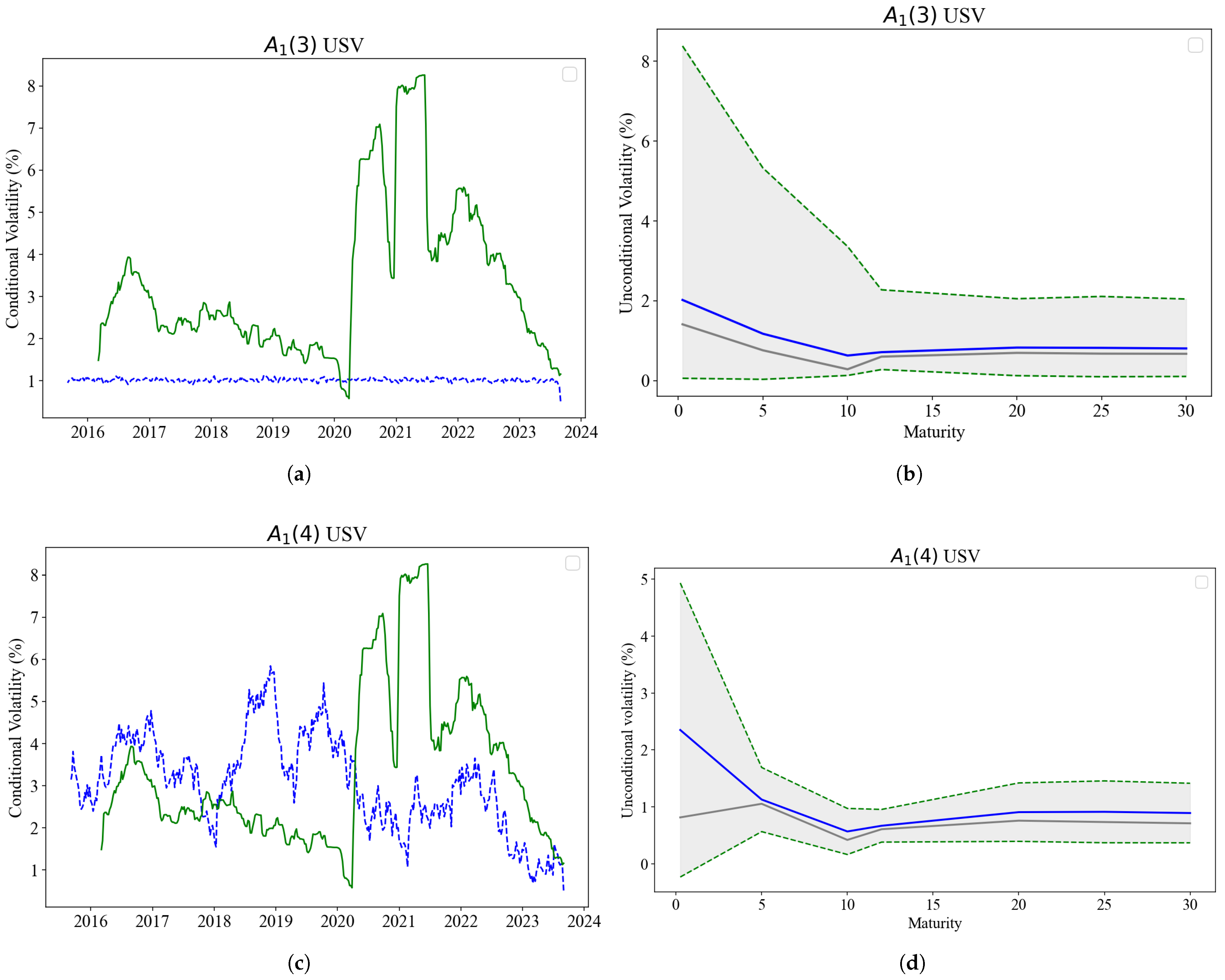
7.3. Time-Series Dynamics
7.4. Volatility Forecasting and Regression
7.4.1. Forecasting and Model Performance
7.4.2. Regression
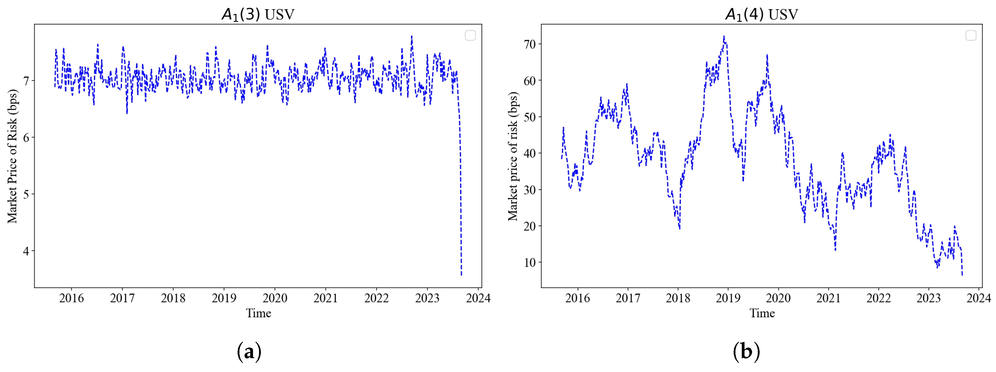
7.4.3. Market Price of Risk
8. Conclusions
Author Contributions
Funding
Institutional Review Board Statement
Informed Consent Statement
Data Availability Statement
Conflicts of Interest
Abbreviations
| ATSM | Affine Term Structure Models |
| BIC | Bayesian Information Criterion |
| BDFS | Balduzzi P, Das SR, Foresi S |
| DM | Diebold–Mariano |
| DK | Duffie and Kahn |
| DTSM | Dynamic Term Structure Models |
| ESS | Effective Sample Size |
| FX | Foreign Exchange |
| GMM | Generalized Method of Moments |
| HDI | High-Density Interval |
| MCSE | Monte Carlo Standard Error |
| MCMC | Markov Chain Monte Carlo |
| LRSQ | Linear-Rational Square-Root |
| MH | Metropolis–Hastings |
| ODE | Ordinary Differential Equation |
| PCA | Principal Component Analysis |
| RMSE | Root-Mean-Square Error |
| SA | South African |
| SME | Simulated Method of Estimation |
| SDE | Stochastic Differential Equation |
| SV | Stochastic Volatility |
| USV | Unspanned Stochastic Volatility |
| USDZAR | SA Rand Dollar |
Appendix A. Derivation of the Physical Measure Drift
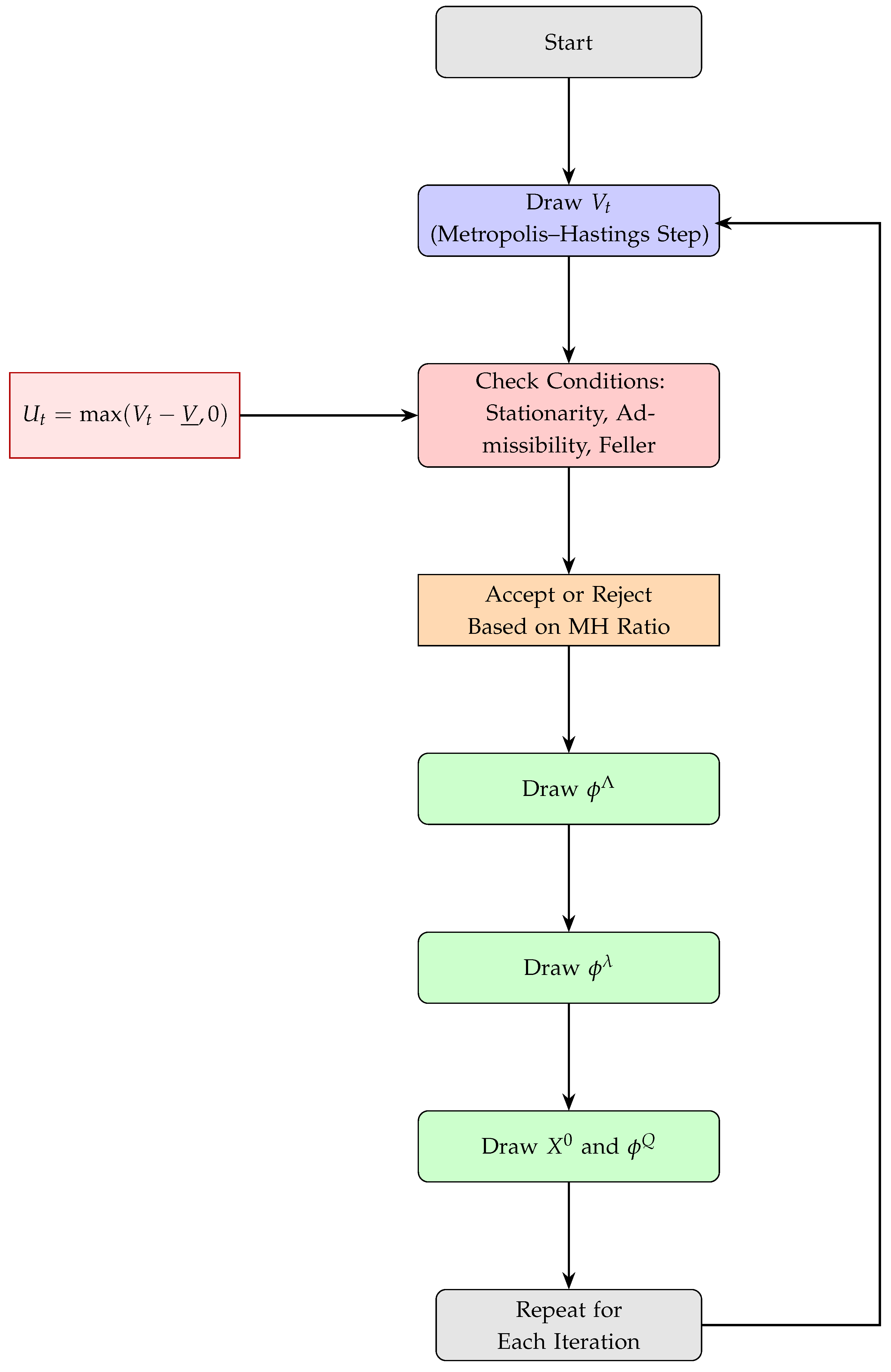
Appendix B. Bayesian Estimation Algorithm
Appendix B.1. Latent State Structure and Volatility
Appendix B.2. Model Discretization
Appendix B.3. State–Space Representation
- : observed yield vector by PC loading, see (23),
- : latent state,
- : observation equation parameters,
- : state equation parameters,
- : state-dependent transition covariance matrix,
- : observation noise covariance.
Appendix B.4. Prior Distributions
- : risk-neutral dynamics parameters,
- : risk premia parameters,
- : measurement error variances.
Appendix B.5. Posterior Structure
Appendix B.6. Sampling Algorithm
- (sampled in blocks),
- (measurement error),
- (risk premia),
- and (risk-neutral dynamics and initial condition),
- (Gaussian latent states).
Step 1: Sampling Ut for t ∈ {1, 1 + h, 1 + 2h,…, T}
- Propose , enforce
- Evaluate acceptance ratio:
- Accept with probability , otherwise retain
Step 2: Sample ϕΛ (Measurement Error)
- Conditional on
- If priors are inverse-gamma, a conjugate update is available
Step 3: Sample ϕλ (Risk Premia)
- Conditional on
- Use MH step if non-conjugate
- Enforce admissibility and stationarity
Step 4: Sample ϕQ and X0
- Conditional on
- Sample via MH or conjugate draw, enforce stationarity
- Sample via conditional normal update
Step 5: Sample (Gaussian Latent States)
- Conditional on all parameters and
- Use Forward-Filtering Backward-Sampling (FFBS) or Kalman smoother
Step 6: Iterate
- Repeat Steps 1–5 for
- Store posterior draws; discard burn-in period
Appendix B.7. Convergence Diagnostics and Tuning
- Acceptance Rate: A reasonable rate is 20–40% in Metropolis–Hastings blocks. Proposal variances should be adjusted accordingly.
- Trace Plots and Autocorrelation: They are used to monitor the mixing behavior of key parameters and latent states.
- Gelman–Rubin Statistic : For multiple chains, verify for all monitored parameters to ensure convergence.
- Effective Sample Size (ESS): It is computed for each parameter to assess how many independent draws are available:where is the autocorrelation at lag k, and S is the total number of post-burn-in samples.
- Highest Density Intervals (HDIs): Use posterior quantiles or kernel density estimates to compute 90% or 95% HDIs:where c is the density threshold that ensures coverage probability .
- Burn-in and Thinning: Discard the first B iterations (e.g., ), where B represents the number of Burn-in iterations. Thinning is optional but may reduce autocorrelation in stored draws. For a detailed discussion on convergence diagnostics, see Roy (2020) and (Kumar et al., 2019) for software applications.
Appendix B.8. Alternative Samplers
- Hamiltonian Monte Carlo (HMC) or No-U-Turn Sampler (NUTS):
- −
- They use gradient information to improve sampling efficiency
- −
- They are particularly useful for high-dimensional latent blocks
- Particle MCMC or Particle Gibbs:
- −
- It is well-suited to nonlinear and non-Gaussian state–space models
Appendix C. Workflow Diagram: Yield Curve Modeling and Inference
Appendix D. Algorithm: Yield Curve Inference via PCA, Kalman and MCMC
| Algorithm A1 MCMC Algorithm with Block Sampling of and Kalman Filtering |
|
| 1 | Collin-Dufresne et al. (2009) decomposes the state variable X into ; where includes all the state variables ,, and , but exclude . The reason is that only affects the factor covariance matrix. They condition on the entire path of, write and in linear-Gaussian state–space form. The draws involving V can be done using relatively inefficient MH. |
| 2 | Risk-neutral parameters and are not identifiable under USV, hence they are replaced by , and (Collin-Dufresne et al., 2009). |
| 3 | We use the Diebold and Mariano (2002) test to assess whether forecast USV significantly outperforms USV in terms of bias and RMSE. The global DM test statistic evaluates the null hypothesis of equal predictive accuracy across the full forecast horizon. Significance is indicated as follows: ** p-value , * p-value , p-value . In addition to the global DM statistic, we compute standardized per-point loss differentials to highlight localized forecast performance differences. Each per-point z-score is defined as: , where is the pointwise difference in forecast losses, is the mean loss difference, and is the sample standard deviation. Significance levels per point are marked by: *** , ** , * |
| 4 | By model-implied volatility we refer to the output from both AND USV models. Readers should not confuse this with the implied volatility surface (option-implied volatility). |
References
- Aït-Sahalia, Y., Li, C., & Li, C. X. (2024). Maximum likelihood estimation of latent Markov models using closed-form approximations. Journal of Econometrics, 240(2), 105008. [Google Scholar] [CrossRef]
- Andersen, T. G., & Benzoni, L. (2010). Do bonds span volatility risk in the US Treasury market? A specification test for affine term structure models. The Journal of Finance, 65(2), 603–653. [Google Scholar] [CrossRef]
- Andreasen, M. M., Jørgensen, K., & Meldrum, A. (2025). Bond risk premiums at the zero lower bound. Journal of Econometrics, 247, 105939. [Google Scholar] [CrossRef]
- Ang, A., Piazzesi, M., & Wei, M. (2006). What does the yield curve tell us about GDP growth? Journal of Econometrics, 131(1–2), 359–403. [Google Scholar] [CrossRef]
- Bikbov, R., & Chernov, M. (2004). Term structure and volatility: Lessons from the Eurodollar markets. SSRN Electronic Journal. [Google Scholar] [CrossRef]
- Cheridito, P., Filipović, D., & Kimmel, R. L. (2007). Market price of risk specifications for affine models: Theory and evidence. Journal of Financial Economics, 83(1), 123–170. [Google Scholar] [CrossRef]
- Christoffersen, P., & Diebold, F. X. (2002, January 2). Financial asset returns, market timing, and volatility dynamics. Market Timing, and Volatility Dynamics. Available online: https://users.nber.org/~confer/2003/si2003/papers/efww/diebold.pdf (accessed on 25 June 2025).
- Collin-Dufresne, P., & Goldstein, R. S. (2002). Do bonds span the fixed income markets? Theory and evidence for unspanned stochastic volatility. The Journal of Finance, 57(4), 1685–1730. [Google Scholar] [CrossRef]
- Collin-Dufresne, P., Goldstein, R. S., & Jones, C. S. (2008). Identification of maximal affine term structure models. The Journal of Finance, 63(2), 743–795. [Google Scholar] [CrossRef]
- Collin-Dufresne, P., Goldstein, R. S., & Jones, C. S. (2009). Can interest rate volatility be extracted from the cross section of bond yields? Journal of Financial Economics, 94(1), 47–66. [Google Scholar] [CrossRef]
- Collin-Dufresne, P., Jones, C., & Goldstein, R. (2004). Can interest rate volatility be extracted from the cross section of bond yields? An investigation of unspanned stochastic volatility. Available online: https://www.epfl.ch/labs/sfi-pcd/wp-content/uploads/2021/07/Can-Interest-Rate-Volatility-be-Extracted-from-the-Cross-Section-of-Bond-Yields.pdf (accessed on 25 June 2025).
- Dai, Q., & Singleton, K. J. (2000). Specification analysis of affine term structure models. The Journal of Finance, 55(5), 1943–1978. [Google Scholar] [CrossRef]
- Diebold, F. X., & Mariano, R. S. (2002). Comparing predictive accuracy. Journal of Business & economic statistics, 20(1), 134–144. [Google Scholar]
- Duffee, G. R. (2002). Term premia and interest rate forecasts in affine models. The Journal of Finance, 57(1), 405–443. [Google Scholar] [CrossRef]
- Duffie, D., & Kan, R. (1996). A yield-factor model of interest rates. Mathematical Finance, 6(4), 379–406. [Google Scholar] [CrossRef]
- Elerian, O., Chib, S., & Shephard, N. (2001). Likelihood inference for discretely observed nonlinear diffusions. Econometrica, 69(4), 959–993. [Google Scholar] [CrossRef]
- Hansen, J. W. (2025). Unspanned stochastic volatility in the linear-rational square-root model: Evidence from the Treasury market. Journal of Banking & Finance, 171, 107354. [Google Scholar]
- Heidari, M., & Wu, L. (2002, September 10). Term structure of interest rates, yield curve residuals, and the consistent pricing of interest rate derivatives. Yield Curve Residuals, and the Consistent Pricing of Interest Rate Derivatives. Available online: https://citeseerx.ist.psu.edu/document?repid=rep1&type=pdf&doi=c708679c36cd86175f128f6fdd5f33ffdc61e959 (accessed on 25 June 2025).
- Johannes, M., & Polson, N. (2010). MCMC methods for continuous-time financial econometrics. In Handbook of financial econometrics: Applications (pp. 1–72). Elsevier. [Google Scholar]
- Kumar, R., Carroll, C., Hartikainen, A., & Martin, O. (2019). ArviZ a unified library for exploratory analysis of Bayesian models in Python. Journal of Open Source Software, 4(33), 1143. [Google Scholar] [CrossRef]
- Litterman, R. B., Scheinkman, J., & Weiss, L. (1991). Volatility and the yield curve. The Journal of Fixed Income, 1(1), 49–53. [Google Scholar] [CrossRef]
- López-Pérez, A., Febrero-Bande, M., & González-Manteiga, W. (2025). Estimation and specification test for diffusion models with stochastic volatility. Statistical Papers, 66(2), 40. [Google Scholar] [CrossRef]
- Piazzesi, M. (2010). Affine term structure models. In Handbook of financial econometrics: Tools and techniques (pp. 691–766). Elsevier. [Google Scholar]
- Riva, R. (2024). How much unspanned volatility can different shocks explain? Available at SSRN 4878175. Available online: https://papers.ssrn.com/sol3/papers.cfm?abstract_id=4878175 (accessed on 25 June 2025).
- Roy, V. (2020). Convergence diagnostics for markov chain monte carlo. Annual Review of Statistics and Its Application, 7(1), 387–412. [Google Scholar] [CrossRef]
- Singleton, K. J. (2006). Empirical dynamic asset pricing: Model specification and econometric assessment. Princeton University Press. [Google Scholar]
- Stroud, J. R., Müller, P., & Polson, N. G. (2003). Nonlinear state-space models with state-dependent variances. Journal of the American Statistical Association, 98(462), 377–386. [Google Scholar] [CrossRef]

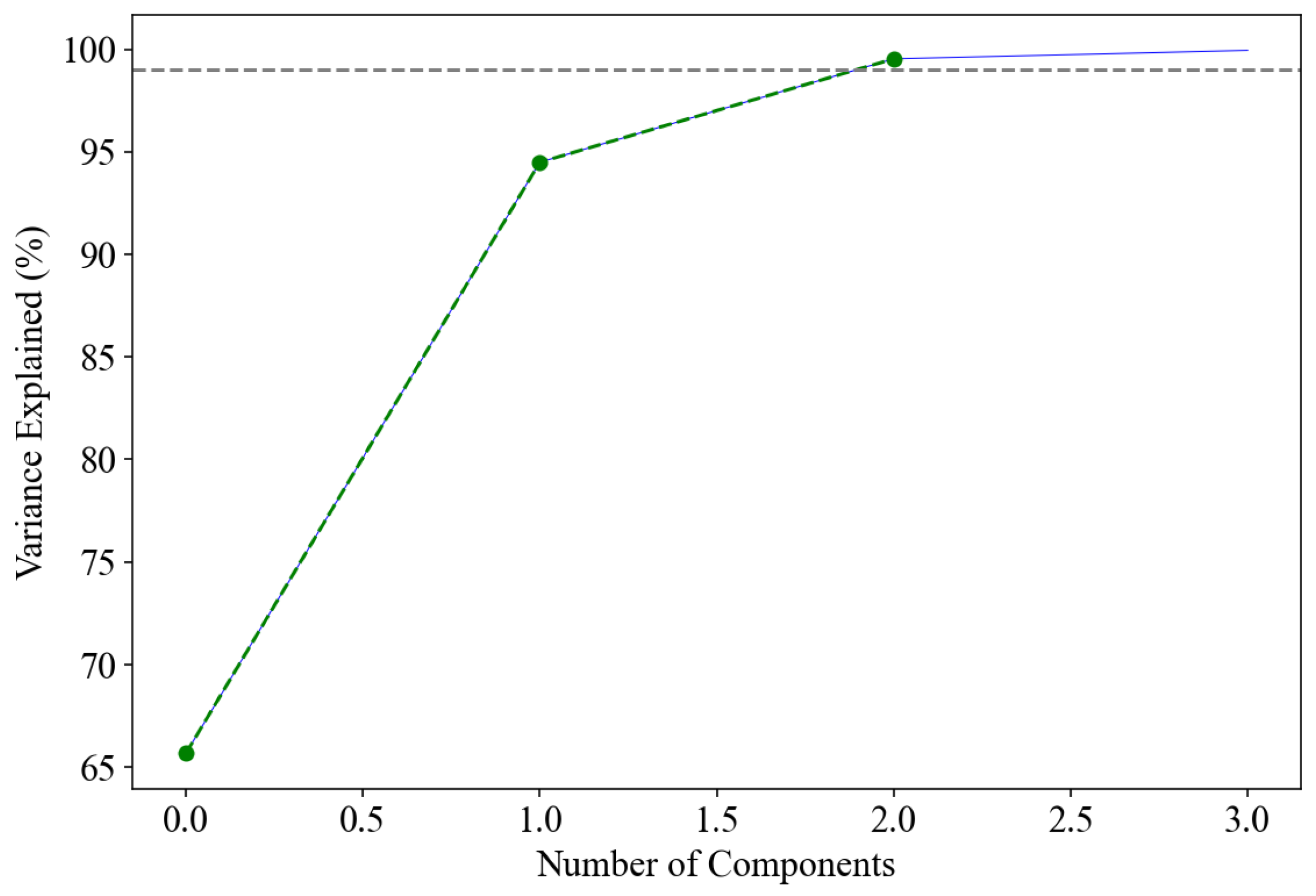
| Principal Components | |||||||
|---|---|---|---|---|---|---|---|
| 1 | 2 | 3 | 4 | 5 | 6 | 7 | |
| 3-month | −0.10 | 0.86 | −0.33 | 0.13 | −0.13 | −0.33 | −0.06 |
| 5-year | 0.02 | 0.36 | −0.08 | −0.50 | 0.44 | 0.58 | 0.28 |
| 10-year | 0.17 | −0.03 | 0.04 | −0.37 | −0.51 | −0.25 | 0.71 |
| 12-year | 0.30 | −0.11 | −0.28 | 0.52 | 0.52 | −0.18 | 0.51 |
| 20-year | 0.60 | 0.00 | −0.37 | 0.21 | −0.43 | 0.50 | −0.15 |
| 25-year | 0.45 | 0.34 | 0.80 | 0.20 | 0.05 | 0.02 | 0.01 |
| 30-year | 0.56 | −0.08 | −0.16 | −0.50 | 0.27 | −0.46 | −0.36 |
| Explained Variance (%) | 66.06 | 30.14 | 3.77 | 0.03 | 0 | 0 | 0 |
| Cumulative Variance (%) | 66.06 | 96.2 | 99.97 | 100 | 100 | 100 | 100 |
| Parameter | (3) USV | (4) USV |
|---|---|---|
| 0.0012 [0.0009, 0.0015] | 0.0010 [0.0010, 0.0010] | |
| −0.3588 [−0.4171, −0.3005] | −0.0780 [−0.1147, −0.0414] | |
| −0.8077 [−1.1711, −0.4443] | −0.0576 [−0.0676, −0.0476] | |
| −0.1113 [−0.1242, −0.0984] | ||
| −0.3152 [−1.0949, 0.4645] | −0.0196 [−0.0203, −0.0189] | |
| 0.0009 [[0.0009, 0.0009] | 0.0020 [0.0019, 0.0021] | |
| 0.4457 [0.4414, 0.4500] | 1.0450 [1.0129, 1.0770] | |
| 0.0071 [−0.0048, 0.0189] | 0.0258 [−0.0230, 0.0746] | |
| 0.0816 [−0.1823, 0.3454] | 0.0190 [0.0016, 0.0365] | |
| 0.0101 [0.0098, 0.0104] | ||
| 0.0003 [−0.0007, 0.0013] | 0.0001 [−0.0000, 0.0002] | |
[, ] | 0.0001 [0.0001, 0.0001] | |
| −0.4622 [−0.5098, −0.4146] | −0.3086 [−0.3226, −0.2945] | |
| −0.0503 [−0.0524, −0.0482] | ||
| −0.0507 [−0.0523, −0.0491] | ||
| −0.0507 [−0.0533, −0.0481] | −0.0973 [−0.1017, −0.0929] | |
| −0.2237 [−0.2456, −0.2018] | −0.0951 [−0.0989, −0.0914] | |
| 0.1043 [0.0992, 0.1094] |
| Parameter | (3) USV | (4) USV |
|---|---|---|
| −0.0122 [−0.0144, −0.0100] | −0.0102 [−0.0104, −0.0099] | |
| −0.0506 [−0.0543, −0.0469] | −0.0478 [−0.0490, −0.0465] | |
| −0.0475 [−0.0524, −0.0427] | −0.0495 [−0.0510, −0.0480] | |
| −0.0098 [−0.0107, −0.0089] | −0.0102 [−0.0105, −0.0099] | |
| 0.0947 [0.0872, 0.1021] | 0.0495 [0.0478, 0.0512] | |
| 0.2783 [0.2518, 0.3047] | 0.1025 [0.0961, 0.1089] | |
| 47.4552 [42.8097, 52.1008] | 10.2594 [9.7983, 10.7205] | |
| −0.0000 [−0.0000, −0.0000] | −0.0001 [−0.0001, −0.0001] | |
| 0.0579 [0.0499, 0.0659] | 0.0941 [0.0890, 0.0992] | |
| −10.5910 [−11.5637, −9.6183] | −1.9671 [−2.0473, −1.8868] | |
| 0.0516 [0.0485, 0.0548] | 0.0201 [0.0196, 0.0206] | |
| 0.0201 [0.0197, 0.0205] | ||
| 0.0193 [0.0183, 0.0203] | ||
| 0.0208 [0.0201, 0.0215] | ||
| 0.0211 [0.0200, 0.0221] | ||
| 0.0193 [0.0181, 0.0204] |
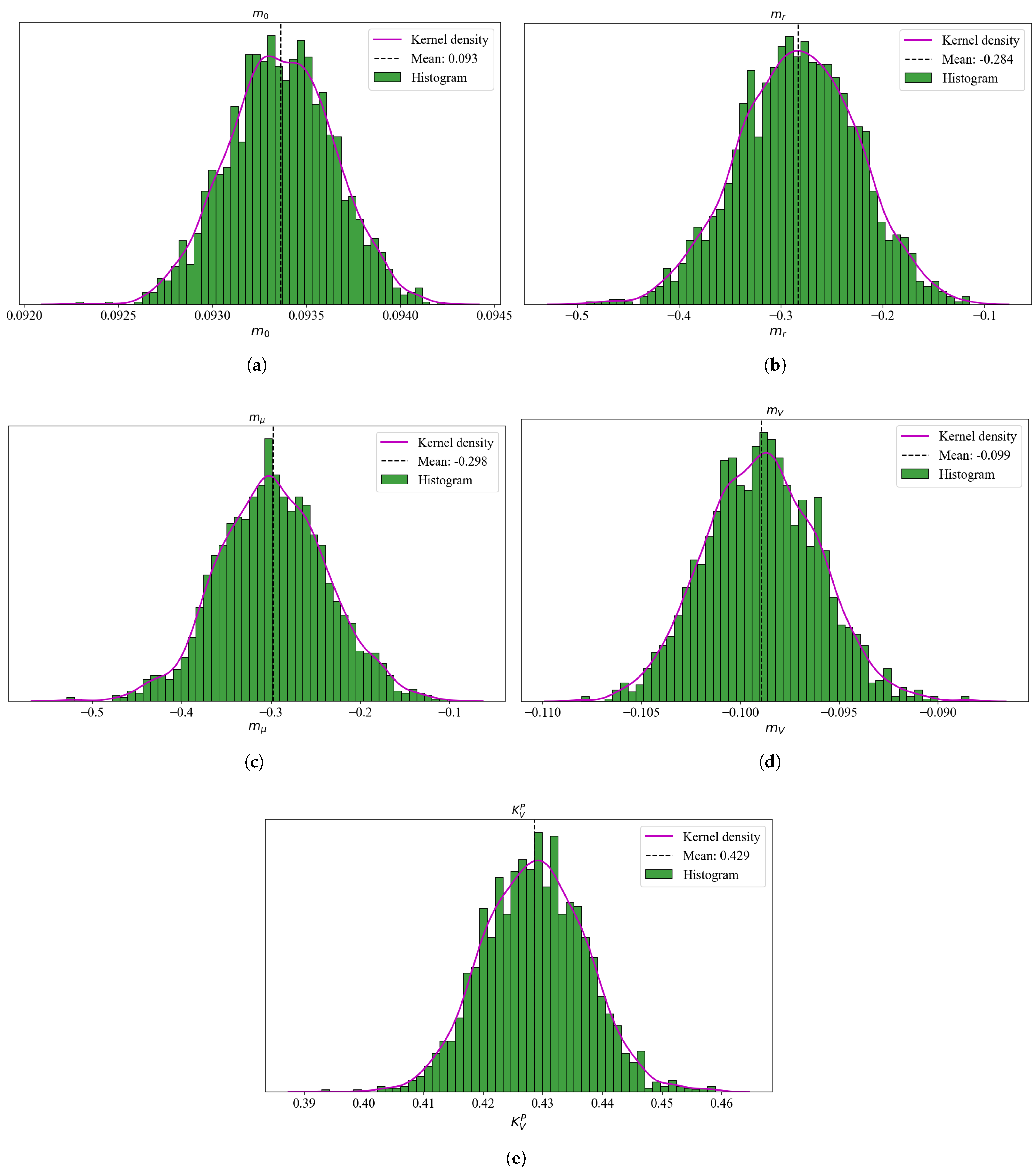
| Mean | Std | HDI (2.5%) | HDI (97.5%) | MCSE (Mean) | MCSE (Std) | ESS (Bulk) | ESS (Tail) | ||
|---|---|---|---|---|---|---|---|---|---|
| 0.001 | 0 | 0.001 | 0.001 | 0 | 0 | 2326 | 1346 | 1 | |
| −0.284 | 0.059 | −0.398 | −0.171 | 0.001 | 0.001 | 2160 | 1106 | 1 | |
| −0.299 | 0.063 | −0.421 | −0.177 | 0.001 | 0.001 | 2555 | 1429 | 1 | |
| −0.099 | 0.003 | −0.105 | −0.093 | 0 | 0 | 2312 | 1495 | 1 | |
| 0.428 | 0.008 | 0.411 | 0.445 | 0 | 0 | 2113 | 1149 | 1 | |
| 0.007 | 0.005 | 0 | 0.016 | 0 | 0 | 975 | 674 | 1 |
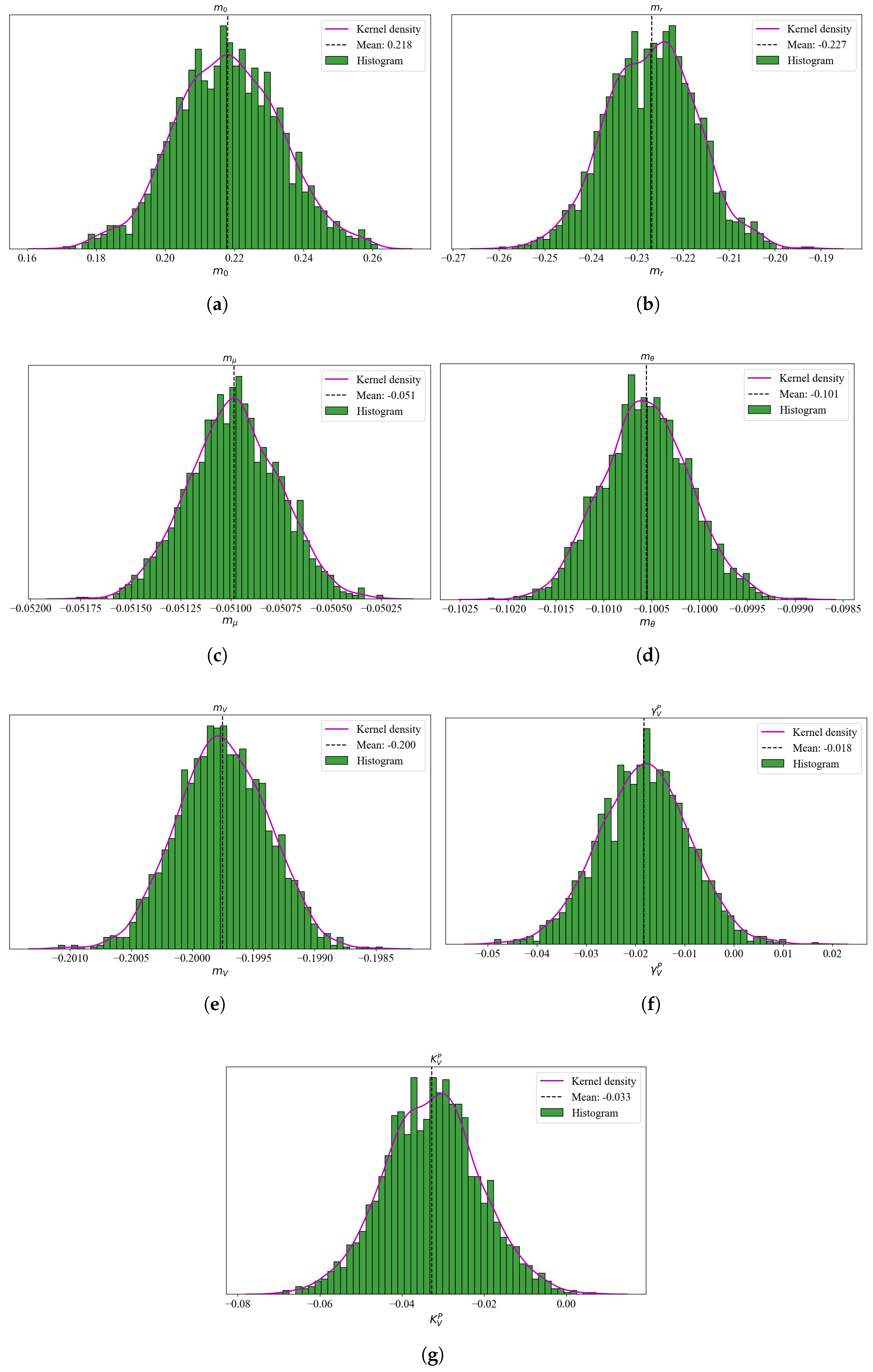
| Mean | Std | HDI (2.5%) | HDI (97.5%) | MCSE (Mean) | MCSE (Std) | ESS (Bulk) | ESS (Tail) | ||
|---|---|---|---|---|---|---|---|---|---|
| 0.093 | 0 | 0.093 | 0.094 | 0 | 0 | 3775 | 1808 | 1 | |
| −0.227 | 0.01 | −0.247 | −0.209 | 0 | 0 | 2626 | 1503 | 1 | |
| −0.051 | 0 | −0.051 | −0.051 | 0 | 0 | 2549 | 1383 | 1 | |
| −0.101 | 0 | −0.101 | −0.100 | 0 | 0 | 2241 | 1407 | 1 | |
| −0.200 | 0 | −0.201 | −0.199 | 0 | 0 | 3182 | 1548 | 1 | |
| −0.018 | 0.009 | −0.036 | −0.001 | 0 | 0 | 2589 | 1617 | 1 | |
| −0.032 | 0.011 | −0.052 | −0.010 | 0 | 0 | 2162 | 1650 | 1 |
| Maturity | USV | Loss Direction | USV | Significance |
|---|---|---|---|---|
| In-sample RMSE 1 | ||||
| 0.25 | 0.0703 | < | 0.0683 | * |
| 5 | 0.0868 | < | 0.0856 | |
| 10 | 0.0958 | < | 0.0946 | |
| 12 | 0.0994 | < | 0.0984 | |
| 20 | 0.1045 | < | 0.1040 | |
| 25 | 0.1053 | < | 0.1043 | |
| 30 | 0.1046 | < | 0.1040 | |
| In-sample bias 2 | ||||
| 0.25 | 0.0660 | 0.0661 | ||
| 5 | 0.0841 | 0.0842 | ||
| 10 | 0.0938 | 0.0939 | ||
| 12 | 0.0978 | 0.0979 | ||
| 20 | 0.1035 | 0.1036 | ||
| 25 | 0.1039 | 0.1041 | ** | |
| 30 | 0.1035 | 0.1036 | ||
| Out-sample RMSE 3 | ||||
| 0.25 | 15.3984 | < | 0.086407 | ** |
| 5 | 0.2219 | < | 0.0896 | |
| 10 | 0.0780 | > | 0.1012 | |
| 12 | 0.0612 | > | 0.1095 | |
| 20 | 0.0389 | > | 0.1233 | |
| 25 | 0.0505 | > | 0.1241 | |
| 30 | 0.0256 | > | 0.1232 | |
| Out-sample bias 4 | ||||
| 0.25 | −12.0832 | 0.0848 | ** | |
| 5 | 0.0855 | 0.0879 | ||
| 10 | 0.0078 | 0.0996 | ||
| 12 | −0.0549 | 0.1079 | ||
| 20 | −0.0369 | 0.1218 | ||
| 25 | −0.0495 | 0.1227 | ||
| 30 | −0.0201 | 0.1218 | ||
| Maturities | 0.25 | 12 | 30 | 0.25 | 12 | 30 |
|---|---|---|---|---|---|---|
| Actual vs. Model Average Yield | 0.964 | 0.964 | 0.964 | 1.000 | 1.000 | 1.000 |
| Actual vs. Model Sope | 0.974 | 0.974 | 0.974 | 0.919 | 0.933 | 0.933 |
| Actual vs. Model Curvature | 0.989 | 0.989 | 0.989 | 0.733 | 0.749 | 0.749 |
| Rolling vs. Model Volatility | 0.054 | 0.002 | −0.037 | 0.550 | 0.157 | −0.049 |
| SA Rand Dollar vs. Model Volatility | 0.007 | −0.024 | 0.058 | 0.408 | 0.122 | 0.613 |
| Brent Crude vs. Model Volatility | 0.050 | 0.064 | 0.000 | 0.216 | 0.055 | 0.478 |
| GARCH vs. Model Volatility | 0.026 | −0.040 | −0.055 | 0.128 | 0.145 | −0.019 |
| Curvature vs. Model Volatility | −0.119 | 0.034 | −0.034 | −0.421 | −0.049 | −0.297 |
| Curvature vs. Model Variance | −0.119 | 0.034 | −0.034 | −0.421 | −0.049 | −0.297 |
| Maturity | USV | Loss Direction | USV | Significance |
|---|---|---|---|---|
| In-Sample RMSE of weekly (bps) 5 | ||||
| 0.25 | 131.83 | < | 37.53 | ** |
| 5 | 50.38 | < | 25.22 | |
| 10 | 39.66 | < | 20.54 | |
| 12 | 31.97 | > | 45.51 | |
| 20 | 27.15 | > | 79.48 | |
| 25 | 27.50 | > | 81.28 | |
| 30 | 26.69 | > | 78.63 | |
| In-Sample RMSE of (bps) 6 | ||||
| 0.25 | 44.68 | < | 39.64 | ** |
| 5 | 28.42 | < | 25.92 | |
| 10 | 26.91 | < | 25.22 | |
| 12 | 26.92 | < | 24.97 | |
| 20 | 27.75 | < | 24.72 | |
| 25 | 26.85 | < | 23.90 | |
| 30 | 27.10 | < | 24.26 | |
| Out-Sample RMSE of weekly (bps) 7 | ||||
| 0.25 | 18.35 | < | 14.87 | |
| 5 | 33.54 | < | 33.22 | |
| 10 | 41.45 | < | 41.39 | |
| 12 | 45.38 | < | 44.91 | |
| 20 | 56.44 | < | 49.60 | |
| 25 | 57.51 | < | 50.00 | |
| 30 | 58.16 | < | 50.18 | |
| Out-Sample RMSE of (bps) 8 | ||||
| 0.25 | 15.60 | < | 14.41 | |
| 5 | 29.58 | < | 28.56 | |
| 10 | 38.52 | < | 37.26 | |
| 12 | 41.57 | < | 40.24 | |
| 20 | 39.71 | < | 38.18 | |
| 25 | 40.57 | < | 38.88 | |
| 30 | 40.56 | < | 38.82 | |
| Variable | Intercept() | Volatility() | Level | Slope | Curvature | |
|---|---|---|---|---|---|---|
| 3-Month Yield Volatilities | ||||||
| GARCH(1,1) | 0.202 [0.015] | 0.395 [0.036] | 0.240 | |||
| 0.210 [0.013] | 0.228 [0.036] | 0.477 | −0.025 [0.005] | −0.112 [0.009] | −0.279 [0.025] | |
| USV | 1.196 [0.2619] | −8.473 [2.576] | 0.027 | |||
| 0.977 [0.203] | −6.876 [1.999] | 0.428 | −0.027 [0.005] | −0.132 [0.009] | −0.334 [0.024] | |
| USV | 0.069 [0.090] | 0.810 [0.274] | 0.022 | |||
| 0.696 [0.126] | −1.321 [0.3956] | 0.427 | −0.043 [0.007] | −0.173 [0.016] | −0.364 [0.025] | |
| 30-Year Yield Volatilities | ||||||
| GARCH(1,1) | 0.068 [0.007] | 0.472 [0.045] | 0.221 | |||
| 0.067 [0.007] | 0.447 [0.045] | 0.241 | −0.005 [0.002] | −0.005 [0.004] | −0.023 [0.009] | |
| USV | 0.350 [0.085] | −2.144 [0.835] | 0.017 | |||
| 0.317 [0.084] | −1.862 [0.8262] | 0.062 | −0.007 [0.002] | −0.006 [0.004] | −0.032 [0.010] | |
| USV | 0.038 [0.025] | 0.302 [0.080] | 0.035 | |||
| −0.293 [0.046] | 1.393 [0.150] | 0.221 | 0.010 [0.003] | 0.037 [0.006] | −0.032 [0.009] | |
Disclaimer/Publisher’s Note: The statements, opinions and data contained in all publications are solely those of the individual author(s) and contributor(s) and not of MDPI and/or the editor(s). MDPI and/or the editor(s) disclaim responsibility for any injury to people or property resulting from any ideas, methods, instructions or products referred to in the content. |
© 2025 by the authors. Licensee MDPI, Basel, Switzerland. This article is an open access article distributed under the terms and conditions of the Creative Commons Attribution (CC BY) license (https://creativecommons.org/licenses/by/4.0/).
Share and Cite
Molibeli, M.; van Vuuren, G. USV-Affine Models Without Derivatives: A Bayesian Time-Series Approach. J. Risk Financial Manag. 2025, 18, 395. https://doi.org/10.3390/jrfm18070395
Molibeli M, van Vuuren G. USV-Affine Models Without Derivatives: A Bayesian Time-Series Approach. Journal of Risk and Financial Management. 2025; 18(7):395. https://doi.org/10.3390/jrfm18070395
Chicago/Turabian StyleMolibeli, Malefane, and Gary van Vuuren. 2025. "USV-Affine Models Without Derivatives: A Bayesian Time-Series Approach" Journal of Risk and Financial Management 18, no. 7: 395. https://doi.org/10.3390/jrfm18070395
APA StyleMolibeli, M., & van Vuuren, G. (2025). USV-Affine Models Without Derivatives: A Bayesian Time-Series Approach. Journal of Risk and Financial Management, 18(7), 395. https://doi.org/10.3390/jrfm18070395