1. Introduction
In the past decades, financial inclusion has become the center stage in the world development agenda as a principal force in the way people are expected to reduce the level of poverty, achieve economic stability, and stability in growth and sustainable development. Financial inclusion is widely defined as access and use of financial services provided through the organized financial system by the entire populace—more so the poor and the vulnerable—has taken position in international policymaking documents such as the Sustainable Development Goals, specifically SDG 8.10. Formidable attention and academic enthusiasm addressed to financial inclusion notwithstanding, large chasms still lay in the understanding of the deeper systemic and structural determinants and mechanisms propelling and constraining financial inclusion in developing economies (
Zulkhibri, 2016). Of great concern is the nexus between financial access and the Environmental, Social, and Governance (ESG) aspects of development, and this still remains a poorly covered area in extant scholarship. This study bridges this significant research gap by developing and testing a new framework to analyze financial inclusion in developing countries using disaggregated ESG measures. Contrary to the mainstream use of the aggregate or unified concept of ESG in the study of sustainability, this study breaks up ESG and its components and estimates their respective contributions to access to finance. More recent scholarship also brings attention to the moderating role played by poverty in the ESG-financial inclusion linkage and the complexities entangled with such interactions (
Jain et al., 2024). Drawing samples from 103 developing countries over a 12-year time frame using comprehensive longitudinal panels from the World Bank and other international institutions’ related datasets, we explore the respective contributions made individually to access to finance by environmental sustainability, social infrastructure, and good governance quality.
The research guiding framework used in this research is
In what way do the Environmental, Social, and Governance components of the ESG framework individually contribute to financial inclusion in developing economies, and how can each such effect reliably be quantified through econometric and machine-learning methods?
We resolve this issue through the adoption of a mixed methodological approach based upon the application of conventional panel econometrics supplemented with instrumental variables methods and advanced machine learning algorithms in order to apply them to regression and cluster analysis purposes. The econometric model allows us to manage the issues related to endogeneity and causality, while the machine learning models, both supervised type (e.g., Random Forest regression) and unsupervised type (e.g., Fuzzy C-Means clustering), reveal profound non-linear relationships and allow countries’ classification according to policy-related categories (
Park et al., 2024).
Our lead financial inclusion indicator is Account Age, the share of adults in a nation who say they have an account at a bank or with a mobile money service provider. This measure has achieved broad consensus as a quantitative proxy for access to the formal financial system and reflects both the penetration of established financial system infrastructure and new digital finance innovations. By considering the effect each of the ESG pillars has separately on Account Age, we will endeavor to build a more nuanced view of the determinants driving financial inclusion in developing economies.
Environmentally, we look at the part played by ecological modernization through proxies such as the use of renewable energy, agricultural production levels and biodiversity conservation, and sensitivity to climatic stress. The concept being that green infrastructure (like solar energy off the grid) can actually promote financial access via facilitation of digital payments in remote areas, while increasing climate risk can increase savings or insurance product take-up (
Xie, 2024). While at the same time, agrarian institution resilience—reflected in high proportions of agricultural land—may indicate structural impediments to financial access in off-grid rural economies.
Along with this, ESG-based analyses have also helped identify risk-mitigated and credible behaviour in individuals and institutions and lending legitimacy to the application of such variables to economic models (
Aghaei et al., 2024). Blending this with our model helps to promote the analytical depth of our machine-learning models and predictive ability in the estimation of access dynamics in the Global South.
On the social side, we apply human development indicators such as education expenditure, internet penetration rates, life expectancy at birth, access to sanitation, and female labor market participation. They are the social capacities upon which financial inclusion depends—i.e., literacy, access to digital technologies, health and well-being, and gender equality. The more advanced the human development in a nation is, the more it is expected to achieve better financial inclusion performance through improved public awareness, institutional trust, and improved ability to make use of financial products and services (
Khalil & Siddiqui, 2020). Social infrastructure is a trigger to access to formal financial services if the digital expansion remains in place.
The governance factor assesses the extent to which institutional quality facilitates or deters access to financial services. Control of corruption, regulatory framework quality, rule of law, and voice and accountability are the measures used to test the hypothesis that good governance creates a facilitative environment for the financial sector to flourish. Governance is at the core of the role played in deciding if citizens are able to access identification systems, if contracts are enforceable or otherwise, and if protection mechanisms work or do not work for consumers, each being a need for a sustainable and inclusive financial system (
Maket, 2024).
To estimate the empirical relations between the aforementioned ESG pillars and financial inclusion, we apply panel data regressions complemented with instrumental variables (IV) in order to counter concerns of simultaneity, measurement errors, and omitted variables. This is particularly imperative in the governance-financial inclusion nexus, where causality might run both ways. Our instruments are drawn from a universe of exogenous ESG-linked variables—such as climate indicators, demographic measures, and environmental stressors—that are correlated with the endogenous regressors but not the error term in the inclusion equation.
We estimate two econometric models: Generalized Two-Stage Least Squares (G2SLS) with random effects and Two-Stage Least Squares with fixed effects. Both are used over a balanced panel of more than 1200 observations to enable robust inference across countries. The need to account for the interdependencies between the variables is further emphasized in recent evidence revealing that income inequality, institution quality, and human development co-determine financial depth and breadth of inclusion in developing countries like Africa (
Kebede et al., 2023).
The econometric evidence is supplemented with a parallel alternative analytical pathway: machine learning modeling, predicting, and classifying financial inclusion levels based on ESG attributes. In this case, we apply a combination of supervised regressions, including Random Forest, Neural Networks, Support Vector Regression, and the use of the Boosting techniques to model predictive performance using the common measures, including Mean Squared Error (MSE), R
2, and Mean Absolute Percentage Error (MAPE). Of the models, Random Forest Regression performs the best and extracts leading non-linear relations and key importances across the variables. More importantly still, the strongest predictors include agricultural productivity (AGVA), renewable energy use (RENE), and the share of areas protected (PROT)—a result eminently derivable from the recent work based on advanced use of machine learning to uncover ESG-finance interlinkages (
K. Li, 2025). In parallel, we apply Fuzzy C-Means clustering—a type of unsupervised use of machine learning—enabling countries to be grouped based on ESG and financial inclusion variables according to soft clusters. This method enables flexible segmentation and the identification of typologies such as “green but excluded,” “socially advanced and inclusive,” and “institutionally weak and financially marginalized.” Such nuanced designations enable both interpretative depth and policy design since countries in the same cluster can, in turn, be addressed with interventions proportionate to their context. The clustering framework also extends the use of the classical econometric analyses since the complex interdependencies and latent patterns characterising the cross-country development context can be accommodated. In yet a further improvement, the use of stacked generalisation techniques using the ensemble methods to aggregate predictive models collectively and achieve greater aggregate robustness is also proving to be beneficial when the aim is to uncover nuanced ESG-finance interaction across different national contexts (
K. Xu et al., 2024). This ensemble method extends the utility in the use of AI-informed insights within financial inclusion analysis, in particular, where policy differentiation according to ESG type is the objective
We recognize each ESG factor to have a distinct and measurable impact on financial inclusion performance. Environmental modernisation—captured through investment in renewables and protection of biodiversity—has a positive relation with financial access, and agrarian economies have a negative relation. Socially, digital access and gender equality measures are the robust positive predictors capturing the reality that digital connectedness and gender-inclusive labor markets are robust enablers of access to the financial system (
Jain et al., 2024). Governance and financial inclusion have a positive relationship, and access to regulation in new forms is where weak regulation remains the inhibitor.
These findings are consistent both across econometric and machine learning methods and are thus more widely applicable across a broad array of developing-country situations. More current innovation in predictive modeling based upon data, such as the inclusion of ESG attributes in financial outcome projections, further legitimizes our approach (
Park et al., 2024).
This research makes three key contributions. First, we provide the first big-data, disaggregate financial inclusion analysis over developing countries based on panel data econometrics and sophisticated machine learning techniques. Second, this study bridges methodological paradigms via the integration of causal inference and predictive modeling to make more nuanced and rich insights available. Third, this study provides recommendations to direct the work of development practitioners, central banks, and multilateral institutions towards the development of context-specific and ESG-driven governance practices to promote financial inclusion. With sustainability, resilience, and inclusion increasingly recognized as interconnected pillars reinforcing one another, it is more and more important to understand the interlinkages between environmental-social-governance and financial access. By incorporating a structured and evidence-based perspective, this study encourages a more holistic understanding of development policy, and financial inclusion is addressed and considered as part of the very core of sustainable development systems rather than as a distinct outcome in itself (
K. Li, 2025).
The article continues as follows:
Section 2 presents the literature review,
Section 3 contains the methodology,
Section 4 presents the relationship between financial inclusion and the E-Environmental component within the ESG model,
Section 5 investigates the relationship between the S-Social component and the ESG model,
Section 6 shows the relationship between financial inclusion and the G-Governance component within the ESG model,
Section 7 analyses the policy implications, the
Section 8 presents conclusions.
Appendix A,
Appendix B,
Appendix C and
Appendix D contain further materials, data, summary statistics, hyper-parameters, and abbreviations.
2. Literature Review
This paper fills basic gaps from the literature at the intersection of financial inclusion and sustainable development by reimagining inclusion as a natural endogenous component of the ESG (Environment, Social, and Governance) framework, rather than a marginal socio-economic end. Financial inclusion has, with almost complete exemption, been studied singly or dyadically with social or environmental indicators. This paper makes a timely addition by providing an integrated ESG-based analytical framework. The literature is notably scarce in theorizing and empirically validating the two-way causal relationships between financial access and all-encompassing sustainability indicators, notably from the perspective of developing regions.
The paper fills the empirical void by employing an extensive macro-panel dataset of 103 emerging markets over 12 years (2011–2022) and therefore permits the temporal dynamics and intra-country heterogeneity to be appropriately controlled. Earlier work is typically cross-sectional or limited-panel specifications, often with poor geographic generalizability. The richness and the breadth of the dataset beget a stronger foundation upon which the structural connection between ESG factors and financial inclusion can be estimated.
Methodologically, the paper makes a contribution by combining instrumental variable techniques with a panel 2SLS approach, using ESG-compatible instruments to control for endogeneity—an issue frequently observed, but hardly forcefully addressed, in the literature. Additionally, the employment of machine learning methodologies, either for regression purposes or for clustering, permits the model to capture complex, non-linear interactions and heterogeneous country configurations better. This blending of approaches distinguishes the study from standard econometric analyses, which assume homogeneity and linearity.
Overall, the paper makes an important contribution by theorizing financial inclusion as a complex vector stimulated by environmental modernization, socio-institutional capability, and the effectiveness of governance. Its findings are in favor of the hypothesis that integrative ESG-financial frameworks are central to the achievement of resilience and fairness in development financing, particularly in the Global South.
The nexus between ESG and financial inclusion in developing countries is a complex and dynamic relationship that acts as a vehicle for sustainable and inclusive development and sustainable finance. Originally conceived as a social goal, financial inclusion as a concept emerged as a cross-cutting force behind all the ESG elements—Environmental, Social, and Governance—where structural disparities and access to finance are weak. According to
Buckley et al. (
2021), FinTech innovations can fill the financial gaps effectively and map financial access with the UN SDGs, while
Chafai et al. (
2024) demonstrate empirically through their evidence that institutional quality through audit quality enhances the ESG impact of financial access in the MENA region. Bibliometric analysis of scholarly fascination with this point of meeting has been presented by
F. Ahmad et al. (
2024), but they do not deeply embed the Global South-specific issues concerned. The emergence of digital technologies accelerated inclusive financing through the confluence of various digital innovations, as noted by
Austin and Rawal (
2023) and
Dhanabhakyam and Suresh (
2024), but innovation creates exclusion and algorithms risks and raises rollout and dissemination ethics concerns as well as fairness concerns over outreach.
Meanwhile, researchers such as
Al-Baraki (
2022) and
Anwar et al. (
2023) stress impact measurement and targeted capital flows and persistent bottlenecks such as gender disparity and lack of formality.
Gonzalez et al. (
2025) emphasize ambitious and comprehensive action at the nexus between climate change, social responsibility, and e-finance access, but their normative perspective might overlook low-capacity bottlenecks. Work such as
Jain et al. (
2024) illustrates the potential through empirical research in ESG and financial inclusion to promote sustainable growth, if the systemic moderator of poverty is addressed.
W. Li and Pang (
2023) and
Khalid et al. (
2024) support the corporate aspect with evidence of digital inclusion mitigating ESG-related conflicts, though
W. Li et al. (
2024) also find that the more pronounced role of greenwashing persists, lowering the efficacy of ESG disclosers.
Halim (
2024) expands the coverage to crowdfunding as a financing conduit and finds disparity across benefits’ distributions. Macro-level research, such as
Hassani et al. (
2024) and
Kiran et al. (
2025), is correlated with financial development and good ESG integration, and
Khan et al. (
2025) explore the enabling role of blockchain and green tech, albeit depending upon international financial integration and equitable infrastructure.
Further operational takeaways are provided by
J. Liu and Naser (
2024), noting increased bank performance—vital in weak economies—as a result of more inclusive finance, reflecting the views of
Malik et al. (
2022), recognizing social sustainability as a stabilizer in the case of Asia. Governance capacity, mentioned by
H. Lu and Cheng (
2024), acts as a mediator between the digital finance ESG effect and
X. Liu et al. (
2024) and
R. Liu (
2024) explore the use of AI by China in order to broaden ESG output, with governance ethics still unresolved as a contradiction. Portfolio-level applications are mentioned by
Lindquist et al. (
2022), with the focus being the incorporation of ESG information within developing economies, and
Mirza et al. (
2025) establishing the connection between ESG-based lending and techno-investments and stability in banks within BRICS economies.
Y. Lu et al. (
2022) recognize the role played by digital inclusion in increasing ESG transparency in the case of China and the EU but warn that those benefits are policy contingent.
On the firm or corporate level,
Pan (
2025) warns of the need for SME-oriented financial tools in digital environments
Roy and Vasa (
2025), using bibliometric analysis, document the trend towards FinTech-powered ESG financing in resource-constrained environments.
Rajunčius and Miečinskienė (
2024) outline a more comprehensive framework blending payment innovation, socially focused equity, and ESG evaluation, and
Shala and Berisha (
2024),
Ravichandran and Rao (
2023) both highlight FinTech’s pivotal role towards ESG progress, but also the potential digital illiteracy risk. Legal foundations are weak institutionally,
Schwarcz and Leonhardt (
2021) remind us and and therefore policy coordination across regions is difficult.
Tekin (
2025) finds Islamic finance to be a culturally resonant model of inclusive ESG in the OIC economies. More advanced ways forward, require the incorporation of well-being goals such as happiness in ESG risk models and require a broader reimagining of the social impacts. Empirical work from
Suresha et al. (
2022) reports financial evidence from Indian markets and illustrates the way in which ESG-matched firms have better financial performance and liquidity, and this supports the materiality of inclusive ESG strategies.
Recent research supports the “S” of ESG—so woefully underrated—is key to sensitive and inclusive financial transformation.
Ubeda et al. (
2023) make this case in the context of the Global South and promote socially-responsible financial models. In the Indian context,
M. Yadav et al. (
2024) and
R. A. Yadav et al. (
2024) discuss the ability of FinTech innovations to diffuse ESG-compatible services to remote zones and lead operations towards sustainability. Empirical evidence from
J. Xu (
2024) and
Xue et al. (
2023) ascertains this alteration in China, too, where ESG performance shifts through the use of AI-guided financial instruments and risk in domains of digitization and accessibility. Rework by
Thomas (
2023) takes a critical analysis of the greenwashing drift in ESG investment and reiterated by
W. Li et al. (
2024), warns that more ESG action will prove pointless if left without accountability mechanisms. Cumulative analysis through bibliometrics by
Trotta et al. (
2024) and
Upadhya et al. (
2024) charts a fractured yet fast-growing body of work wherein FinTech emerges as a key enabler in re-locating the arena of ESG debate. Though momentum gathers,
M. Yadav et al. (
2024) warn that without coordination through policy and enabling infrastructures, and importantly in the remote areas, the transformational potential of digital financial expansion through ESG models remains unrealized.
A synthesis of the literature review is presented in the following
Table 1.
3. Methods and Data
The study selects a hybrid methodological design involving econometric estimation with instrumental variables (IV) and machine learning (ML) techniques for the purpose of assessing the relationship between financial inclusion and ESG (Environmental, Social, and Governance) dynamics for 103 developing countries over the period 2011–2022. Due to the extensive and complete set of variables utilized over the entire investigation, detailed descriptions, definitions, and sources are placed in the
Appendix A,
Appendix B,
Appendix C and
Appendix D, with the aim of simplicity over the entire primary text. The dependent variable, financial inclusion, has been proxied by the “Account Age” indicator, the share of adults with an account maintained at a formal financial institution, or with a cell money service. The variable was obtained jointly from the World Bank Databank and the Sovereign ESG Data Portal with the aim of ensuring accuracy and cross-country comparability (
Hicham & Hicham, 2020;
Eldomiaty et al., 2020). The World Bank’s harmonized ESG dataset provides the ESG indicators, also disaggregated by the environment, social, and governance pillars. The econometric estimation utilizes both the Generalized Two-Stage Least Squares (G2SLS) and Fixed Effects Two-Stage Least Squares (FE-2SLES) estimators while overcoming endogeneity, measurement error, and simultaneity bias, common problems at the macro level of development research (
Jain et al., 2024). Instrumental variables such as climate stress measures, sanitation infrastructure, and demography-based controls have been selected for their exogeneity. Diagnostic tests indicate strong model performance, with the levels of R
2 reaching 35% in the environment specification and statistically significant Wald χ
2 tests (
p < 0.001), supporting strong explanatory strength and instrument credibility (
Chininga et al., 2023;
Gidage & Bhide, 2025). For the machine learning approach, supervised regression models have been implemented towards the discovery of a non-linear relationship between ESG dimensions and financial inclusion. An evaluation has been performed comparatively between eight algorithms: Boosting Regression, Decision Tree Regression, K-Nearest Neighbors Regression, Linear Regression, Neural Networks, Random Forest, Regularized Linear Regression, and Support Vector Machine. This supports the reliability of ensemble-based models towards the discovery of non-linear, hierarchical associations pervasive with ESG-based datasets (
K. Li, 2025). For unsupervised learning, the five clustering analyses implemented were Fuzzy C-Means (FCM), Hierarchical Clustering, Model-Based Clustering, Neighborhood-Based Clustering, and Random Forest-based proximity clustering. As the most appropriate approach, FCM was selected by optimal performance from an exhaustive set of cluster validation indices: R
2, Akaike Information Criterion (AIC), Bayesian Information Criterion (BIC), Silhouette Score, Maximum Diameter, Minimum Separation, Pearson’s γ, Dunn Index, Entropy, and the Calinski-Harabasz Index. FCM’s soft clustering properties are well-suited for extracting the overlapping ESG-financial inclusion characteristics ubiquitous in most developing economies, therefore enabling finer policy segmentation (
Waliszewski, 2023). Merging causal econometric models with machine-learning-based classification permits an inclusive, scalable, and evidence-based framework for questioning financial inclusion with regard to ESG configurations. It offers explanatory rigor and tractable knowledge through the determination of archetypal country profiles, thus informing the generation of more tailored, context-sensitive policy interventions designed to support sustainable development.
Approximately 12% of the dataset, covering 2011–2022, exhibited missingness. These were imputed by cross-sectional mean imputation. For the fairly limited panel duration of 11–12 years, the approach was considered a pragmatic compromise, avoiding significant loss of data while maintaining continuity for the dataset. While appropriately noted that imputation by the mean can attenuate variance and distort correlations, in turn potentially reducing coefficient estimates or suppressing associations between variables, it also possesses the advantages of simplicity, transparency, and computational ease. In the case of sample size maintenance, the top priority and the missingness not being structured in a systematic manner, mean imputation can be a fair compromise. Accordingly, while we take note that with the use of advanced approaches such as multiple imputation or time-series imputation, there are potential improvements by way of robustness, the approach selected is commensurate with the structure and scope of the current dataset.
4. Sustainable Finance and Environmental Resilience: Modelling Financial Inclusion Through the “E” in ESG
This empirical analysis investigates the relationship between environmental sustainability and financial participation in developing nations through the proxy Account Age as a measure of participation in financial services. As financial access is rapidly emerging as a central driver of inclusive growth, it has become imperative to investigate the manner in which the environment and environmental considerations shape such access. Under the ESG (Environmental, Social, Governance) framework, the current study focuses on the “Environmental” pillar and examines the effect of six significant environmental variables on a multi-period panel dataset. To address the possible issue of simultaneity or endogeneity, both G2SLS (Generalized Two-Stage Least Squares) and TSLS (Two-Stage Least Squares) specifications are used in estimation and yield statistically reliable results. Prior research supports the use of environmental indicators such as renewable energy use and land quality in studying the financial inclusion-environment nexus (
Jain et al., 2024). The overall goal is to provide empirical insight helpful for sustainable policy making and show that well-designed environmental policies can also enhance financial participation. Recent findings show that digital financial inclusion can inhibit greenwashing while strengthening authentic ESG performance, supporting the idea that financial access and environmental responsibility can reinforce each other (
W. Li et al., 2024). Moreover, inclusive finance is shown to improve environmental quality through enhanced service accessibility and reduced household vulnerability, especially when financial systems are aligned with ecological priorities (
Wang et al., 2022). The findings establish positive synergies between economic access and climate resilience and suggest that environmental stewardship will not be a restraint but rather a facilitator of sustainable and inclusive development (
Table 2).
The principal goal of this empirical research involves investigating the connection between financial inclusion, as captured by the measure used here for this research—namely, the Account Age variable—defined as the proportion of those who reported having an account (in their own right or jointly) at a bank or other type of financial organization or who used a mobile money service themselves in the previous year—against a set of environmental variables collected together as representing the “Environmental” part of the ESG approach (Environmental, Social and Governance). The analysis will be confined exclusively to developing countries since their countries present specific differences in their structural, socio-economic, and institutional contexts in relation to high-income economies and since their levels of financial inclusion and success or prominence of environmental policies largely depend on them.
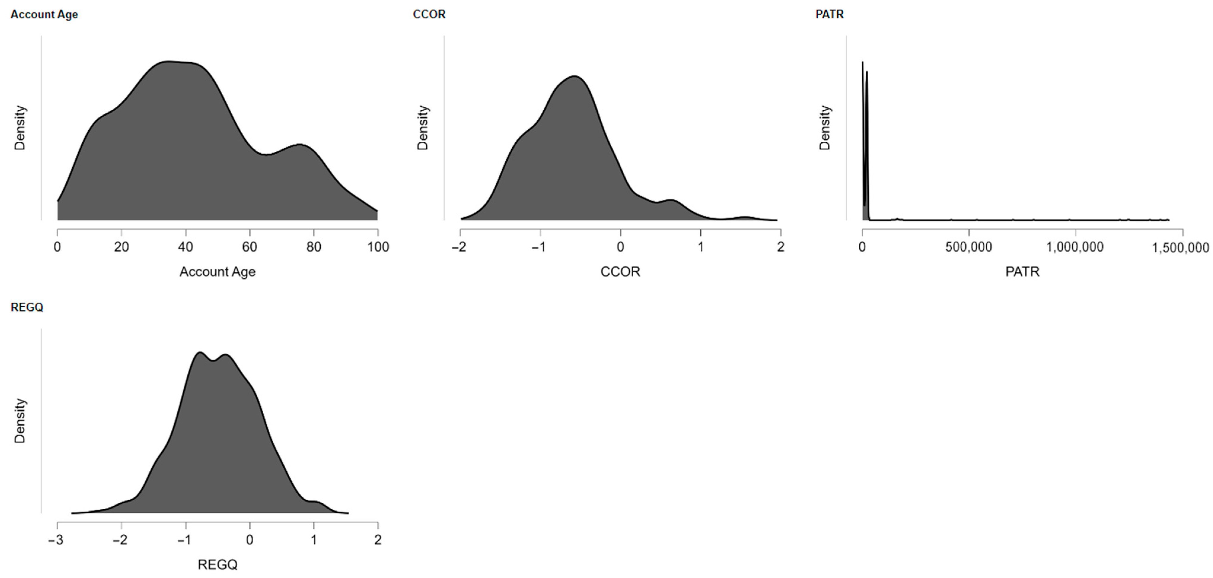
The empirical approach employs six explanatory variables with close links to the Environmental pillar of ESG: (1) AGRL—agricultural land as a percentage of total area, (2) AGVA—value added in agriculture, forestry, and fisheries as a percentage of GDP, (3) FOOD—food production index, (4) HIDX—heat index of the number of days on which the apparent temperature rises above 35 °C, (5) RENE—share of consumption of renewable energy as a percentage of total energy consumption, and (6) PROT—protected areas on the land and seabed as a percentage of total territorial area. The variables were employed since they capture key environmental dynamics for developing countries and should impact financial inclusion directly or indirectly.
The empirical specification employs two instrumental variable forms in order to take account of potential endogeneity: a G2SLS (Generalized Two-Stage Least Squares) random effects and a TSLS (Two-Stage Least Squares) fixed effects specification. The two specifications share a balanced panel of 1235 observations covering 103 countries over a time series ranging from 11 years to 12 years in duration. The use of instrumental variables serves as a necessity in order to address issues related to simultaneity-based endogeneity concerns, omitted variable bias, or measurement error. The instruments used are diverse and potent and include human development proxies (e.g., access to electrification and the internet, literacy rate, school enrolments), public health indicators (e.g., access to sanitation and clean water and under-5 mortality rate), demographic variables (e.g., crude population density and proportion of the age group 65 and above), and governance-quality variables (e.g., control of corruption sub-indices and sub-indices of rule of law, regulatory quality, and voice and accountability).
Both models yield the same results and are statistically significant, and consistently depict a clear understanding of the effects of environmental variables on financial inclusion in developing countries. The AGRL (land area used for agriculture) variable has a negative and highly significant relationship to financial inclusion in both models (G2SLS: −0.593, z = −4.213 and TSLS: −0.698, z = −4.814). It reflects countries with large agricultural land areas having lower financial inclusion. It may be a reflection of domination by agrarian economies and informal economies, where financial institutions remain underdeveloped and formal financial services and instruments remain limited. The same holds true for the AGVA variable—value added through agriculture, forestry, and fish—referring a negative and significant relationship (G2SLS: −1.975, z = −6.406 and TSLS: −0.735, z = −1.887), supporting the argument that agrarian economies without integration or modernization do not integrate or become included in financial systems.
On the other hand, other environmental variables show a positive and significant relationship. The FOOD variable (index of food production) has a positive and significant relationship in both models above (G2SLS: 0.412, z = 5.704; TSLS: 0.444, z = 7.250). It reflects the fact that in countries where levels of agricultural productivity tend to be stronger, the inhabitants tend to be in contact with financial institutions more often. This can be justified by the reasoning that a higher food production level may foster well-organized value chains, contract farming, agricultural insurance, and microcredit availability, and thus encourage demand for financial products and services as well as both demand- and supply-push motives for financial institutions. Likewise, the HIDX variable (heat index) also shows a positive and significant relationship (G2SLS: 0.376, z = 2.933; TSLS: 0.481, z = 3.565). This may be less intuitive and may be a sign of adaptation behavior: in countries with high frequencies of extreme weather conditions, investment in resilience may be enhanced, and thus, maybe the take-up of digital financial means such as climate insurance or environmental shock coping savings accounts.
The other significant finding relates to RENE (consumption of renewable energy), which has a positive and statistically significant coefficient on both specifications (G2SLS: 0.140, z = 3.125; TSLS: 0.120, z = 2.919). The correlation might be driven by the increasing penetration of renewable energy facilities, such as off-grid mini-grids and photovoltaic panels, in remote villages and small towns. These systems would be based on digital payment systems (e.g., pay-as-you-go solar) and funded by microfinance or leasing schemes, which in turn create an incentive for opening a financial account or the use of mobile money services on the part of the consumers (
Ababio et al., 2023).
The PROT variable, which accounts for the proportion of protected areas, has the strongest positive correlation with financial inclusion (G2SLS: 1.505, z = 7.389; TSLS: 1.376, z = 7.652). The finding can be explained through the prism of inclusive environmental governance: if active conservation policies take effect, they tend to be grounded on community participation, formalized funding channels, and coordination between NGOs and external institutions, which may stimulate access to financial services in local communities (
Paliienko & Diachenko, 2024).
Both estimations from a model performance perspective hold good explanatory power. The R2 measure of determination approximates 34.5% for the G2SLS and approximately 34.7% for the TSLS fixed effects method, hence explaining a good percentage of variance in the Account Age indicator. Additionally, the Wald test for the collective explanatory significance of the explanatory variable produces highly significant values (χ2 = 457.6 for G2SLS and χ2 = 491.9 for TSLS; both p < 0.001), confirming the statistical validity of the models.
In short, this analysis offers systematic and strong empirical evidence that the environmental dimension of ESG has a crucial impact on the level of financial inclusion in developing countries. Precisely, those traditional and underdeveloped agricultural system-related variables tend to behave in a negative correlation manner vis-à-vis formal access to financial services. However, those environmental variables related to productivity, resistance, accessible sustainable energy, and policy enforcement of conservation efforts tend to be correlated in a positive manner vis-a-vis better levels of inclusion (
Dovbiy, 2022).
These findings are most directly relevant for policymakers and development institutions as they reveal the complementarities between access to finance and environmental sustainability. Encouragement of environmentally sustainable behavior may not only be beneficial from an environmental angle but also may entail economic and societal spillovers through enhanced coverage of financial services by previously under-banked groups.
With regard to the 2030 Agenda of Sustainable Development and in particular in relation to SDG 8 (Decent Work and Economic Growth) and SDG 13 (Climate Action), this study contributes to an emerging literature on the means through which environmental factors may be leveraged as drivers of inclusive economic growth. The cross-cutting ESG approach taken by this research calls for a holistic development comprehension whereby environmental stewardship is not a constraint but an accelerator of inclusive, resilient, and sustainable financial ecosystems in the Global South. The determined correlation between the “E” of ESG and financial inclusion means policies must be couched so they may address simultaneously both climate resilience and economic access, and consequently achieve synergies that promote both ecological integrity and social equity.
To gauge the strength and relevance of the instrumental variables used for the 2SLS estimates, first-stage regressions were performed separately for each of the six endogenous variables: AGRL, AGVA, FOOD, HIDX, RENE, and PROT. These first-stage regressions yielded some valuable diagnostics--R-squared measures, F-statistics, and the number of statistically significant instruments--that represent a good check of the quality of the instruments. The results are that the instruments have substantial explanatory power for the great majority of the regressors. For five of the six, the F-statistics are well over the standard 10 threshold, with particularly high values for AGVA (55.56), HIDX (34.32), and RENE (95.76), definitively ruling out the potential for weak instruments. The only exception here is the situation of FOOD, with an F-statistic value of 9.27, just below the threshold, indicating a low probability of weak instrument bias, for whose respective second-stage estimate(s) some interpretive circumspection is merited.
The instruments also have substantial explanatory power through the course of models, with R-squareds from 0.19 for FOOD to 0.70 for RENE. At least eleven 5 percent significant instruments are reported for each regression, while between five and thirteen instruments are 1 percent significant. For instance, the instruments EDUE, CFTC, LIFE, PDEN, and REGQ are significant predictors for AGRL, while RENE is associated with a long list of highly significant instruments like CFTC, LABR, POP6, and some of the governance indicators. These patterns confirm the observation that the instruments are not only statistically significant, but also strongly associated with the endogenous regressors they try and illuminate. Complete first-stage regression tables are also reported in the
Appendix B to aid transparency and the ability to replicate (
Table 3).
4.1. Financial Access in the Climate Era: A Cluster-Based Exploration of Environmental-Economic Interactions
This section presents advanced clustering analysis aimed at revealing dynamics between environmental and financial variables in developing countries through the use of the Fuzzy C-Means method. The countries were grouped by similarity in the six environmental indicators and the Account Age measurement as a proxy measure of access to financial services. The nine-cluster solution based on the best statistical fit as well as interpretability was finalized. The cluster analysis presents divergent profiles and illustrates ways in which environmental participation, agricultural organization, and proportion of renewables intersect with participation stages in the economy. The results offer actionable insights in the complex and sometimes patchwork relationship between economic participation and sustainability in the Global South (
Table 4).
Among the cluster algorithms we experimented with—Density-Based Clustering, Hierarchical Clustering, Model-Based Clustering, Neighborhood-Based Clustering, Random Forest Clustering, and Fuzzy C-Means Clustering—the latter’s Fuzzy C-Means method emerged as the best-placed and efficient method based on a multi-metric performance assessment (
Kaushal et al., 2024). By normalizing and comparing twelve performance measures—compactness measures and cluster validity and separation measures alike—FCM produced the highest mean performance score, pointing towards FCM as the method typically superior in this use case.
One of the great strengths of FCM as a technique is its ability to accommodate data points being part of several groups to any extent of membership. This soft type of clustering method is very useful with complex data where different groups may lack distinct boundaries. In contrast with hard clustering methods such as k-means, where each point is assigned exclusively to a particular group, FCM captures more subtle patterns in the data and provides more interpretability and flexibility (
L. Zhang et al., 2020). FCM’s flexibility is evident in the very high performance across all significant parameters, such as the R
2 value (0.84), reflecting the variance accounted for in the case model, and the silhouette score (0.56), reflecting good cluster separation and cohesion.
FCM achieved a 1.0 normalized value in our comparison experiment in terms of the Calinski-Harabasz index, Entropy, and Clusters. The measure of the Calinski-Harabasz index measures the ratio of between-cluster variance and the within-cluster variance, and a high value reflects well-separated and compact clusters. Achieving a 1.0 value in this case provides a clue that FCM developed compact and well-separated clusters. Entropy measure in clustering can reflect randomness or uniformity in cluster assignment distribution, and also achieves a maximum score in the FCM case. A value of 1.0 means FCM achieved high consistency in the clustering structure. That it also scored 1.0 in Clusters means the number of achieved clusters lies at the optimum or very near the optimum value to be expected in the dataset (
Shen et al., 2021).
In addition, FCM performed comparably on other key measures, too. On the measure for the minimum between-clusters distance and the maximum within-clusters diameter in the form of the Dunn index, FCM value at 0.04 can also be considered low but comparable, since the maximum value 1.0 could only be achieved by the Density-Based Clustering method alone. FCM scored 0.54 at Pearson’s γ, the measure of the distance between points and the degree to which the points belong to the same cluster or different ones, being behind Hierarchical Clustering alone at 1.0 when it comes to its score in this measure. This reflects good geometric form preservation of the data through FCM. Even in the case of Minimum Separation and Maximum Diameter, measuring the distance between the clusters and the size of the largest cluster, respectively, FCM retained a good measure and proved to have good compactness and well-separateness simultaneously.
Both Neighborhood-Based Clustering and Hierarchical Clustering did well on both measures—a silhouette score of 0.68 and 0.84, respectively—but were far from as reliably high-performing as FCM. The levels of R
2 were lower both times (0.53 and 1.0, respectively), but both algorithms scored 0.0 on important measures such as the Calinski-Harabasz index, AIC, and BIC, indicative of their potential inefficiencies in model selection and complexity penalty. FCM’s mean overall score of 0.58 is indicative of a well-balanced performance without falling low on any of the measures provided (
Paliienko & Diachenko, 2024).
The key point also resides in good interpretability in high-dimensional spaces, and this makes FCM a good choice for exploratory analysis in bioinformatics, segmentation of the market, and image classification. Its use of fuzzy logic also aligns with the reality of the overlapping classes and imprecise groupings in the real world. In practical terms, this can lead to actionability over strict partitioning algorithms.
Fuzzy C-Means Clustering outperforms in performance based on good cluster compactness and separability, and model validity, as well as being more flexible and interpretative. Its highest mean score of the algorithms considered speaks volumes about the flexibility and potency of the algorithm. No cluster method is its best across all measures, yet since FCM performs well across a range of measures over and over again, it is the optimum method for this dataset. This conclusion, based upon empirical performance, is further enriched through the theoretical advantages of the algorithm’s capacity to accommodate fuzzy boundaries and preserve the internal organization of the data. (
Table 5).
Fuzzy C-Means clustering outputs reveal a sharp segmentation of countries (or regions) based on the interaction between financial inclusion in terms of Account Age and a range of environmental variables within the E (Environment) corner of the ESG framework. Cluster analysis, within the developing country context, shows the nexus between financial infrastructure and environmental engagement, resilience, and sustainability (
Zioło et al., 2022). The variables employed are AGRL (land used for agriculture), AGVA (agriculture, forestry, and fishery value added), FOOD (% food production index), HIDX (% heat index 35), RENE (% renewable energy consumption), and PROT (% terrestrial and marine protected areas). The overall goodness of fit of the clustering model as a ratio of BSS/TSS at circa 44.3% reflects significant but relative capture of the heterogeneity and supports significant overlapping country profiles (
López-Oriona et al., 2022). Financial inclusion perspective-wise, Cluster 2 (with the highest proportion explained at 25%) possesses a moderately high Account Age (0.450) and high environmental responsibility through PROT (1.100), but low values in RENE (−0.903) and AGVA (−0.813). This might reflect the regions with good institutions and conservation systems, but poorly developed renewables and agri-economies. Cluster 4, with its high values in both AGRL (1.417) and AGVA (1.592), overtly reflects regions with a high agrarian core. The Account Age in this case surprisingly emerges as negative (−0.667), and this reflects that even agri-advanced areas and financial service bottlenecks might arise. This contrast indicates an economic activity-financial access mismatch and a key development bottleneck. Cluster 9 comprises the smallest number of companies (only 25) but is striking in the high level of environmental responsibility: PROT (1.593), RENE (−1.115), and positive Account Age (0.317). Its relatively low renewable energy consumption is inconsistent with high levels of biodiversity conservation. The fit may be the result of conservation policies advocated and pursued by the state within those contexts where green technologies are still inaccessible. Group 1 possesses a clear profile of weaknesses: very low Account Age (−1.512), lower usage of renewable energy (−1.412), and minimal protection of the environment (−1.146). It has moderately high AGVA (0.995) but extremely low financial cover and heat stress (HIDX = 0.779), corresponding to climate-vulnerable and institutionally undercovered locales. Cluster 6 is a very interesting paradox. It has the largest RENE (1.914) and positive PROT value (0.317), yet very low Account Age (−0.848) and AGRL (−1.577). This corresponds to green transformation at the nascent stage—possibly driven by donors or technologically enabled—in a context of limited classical agriculture and minimal access to finance. This might reflect the case of countries turning to renewables while no overall financial safety net exists for their populations (
Azkeskin & Aladağ, 2025). Cluster 3 shares the middle Account Age (−0.546) and relatively evenly distributed environmental values, specifically RENE (0.207), and therefore can be deemed middle-ground segment with lower variablity since it also witnessed lower explained heterogeneity (4.1%) and highest silhouette value (0.222), being a dense and homogeneous segment. Cluster 5, being the largest cluster with 326 units, contains mixed attributes: Account Age (−0.185), AGVA (−0.569), and barely better-than-average FOOD (0.596), yet both negative RENE (−0.370) and PROT (−0.364). These contradictory bits of information suggest a type of profile of the “developing majority”—economies with modest food-producing capacity but low ecological and financial inclusion levels. Cluster 8 possesses low FOOD (−1.943) and Account Age (0.302) and below-average readings in all other measures. Its small size (N = 62) and low value of the silhouette (0.128) indicate it might include outliers or the economies in the process of transforming towards the outside conditions. Finally, Cluster 7, whose values are close to the mean, specifically in RENE and PROT measures (0.255 and −0.365), might serve as a “benchmark” profile—neither too underdeveloped and yet high performances are below its level yet also far from the highest level and thus it still has room to develop and improve both the fiscal and the environmental fronts. On the whole, the clustering shows financial access does not have high intercorrelation across environmentally varied segments in developing countries. Conditions in agriculture and the environment do not directly correlate with high financial access and vice versa. The framework pushes the importance of the integration planning financial access and the environment in the first place in areas exposed to climate risk or sustainability transitions. The findings support the unified ESG strategy where social infrastructure (i.e., access to banks) should never be decoupled from green investment, particularly in emerging and vulnerable economies (
Table 6).
The outcomes from Fuzzy C-Means clustering present a refined breakdown of countries (regions) according to the interaction of financial inclusion, as quantified by Account Age, and a set of environmental variables taken from the E (Environment) pillar of the ESG framework. The clustering analysis in the developing countries context shows the relationship between environmental engagement, resilience, and sustainability, and financial infrastructure (
Latifah, 2022). The variables used comprise AGRL (agricultural area), AGVA (agriculture, forestry, and fishing value added), FOOD (index of food production), HIDX (heat index 35), RENE (consumption of renewable energy), and PROT (land and ocean and island protected areas). The global fit of the clustering model, wherein the ratio of the Between Sum of Squares (BSS) and the Total Sum of Squares (TSS) is about 44.3%, shows that the nine-cluster solution accounts for a considerable but not full extent of the heterogeneity and therefore indicates meaningful although overlapping country profiles (
Sasmita et al., 2023).
From a financial inclusion viewpoint, Cluster 2 (the largest proportion explained at 25%) has a moderately high Account Age (0.450) and high environmental concern through PROT (1.100), but low scores on RENE (−0.903) and AGVA (−0.813). This may indicate those regions with good institutions and conservation policies, but not well-developed renewable infrastructures and agricultural economies. Cluster 4, having high scores in AGRL (1.417) and AGVA (1.592), evidently locates regions having a well-established agricultural base. The Account Age here remains surprisingly negative (−0.667), however, and may indicate that even agriculturally developed regions will be encumbered by access to financial services. This gap reflects a disconnect between economic activity and access to finance, a key development bottleneck.
Cluster 9 has the lowest number (only 25) but has a strong environmental orientation: PROT (1.593), RENE (−1.115), and positive Account Age (0.317). Paradoxically, although it has minimal use of renewables, it has excellent biodiversity preservation. The cluster might be a reflection of government-run policies for conservation in areas where green technologies remain inaccessible.
On the other hand, Cluster 1 has a definite outline of vulnerability profile: extremely low Account Age (−1.512), low levels of renewable energy consumption (−1.412), and low levels of environmental protection (−1.146). It has a moderately high AGVA (0.995) but low levels of financial inclusion and heat stress (HIDX = 0.779), reflecting climate-vulnerable, institutionally underserved areas.
Cluster 6 presents a very interesting contradiction. It has the largest RENE (1.914) and a positive PROT (0.317) score, but very low Account Age (−0.848) and AGRL (−1.577). This indicates an early-stage green transition—potentially technologically enabled or donor-driven—wherein there is low traditional agriculture and limited financial coverage. This may be representative of those countries adding or embracing renewables without a general financial cushion of safety in their populations (
Bondarenko et al., 2025).
Cluster 3 has a medium Account Age (−0.546) and fairly well-balanced environmental values, primarily RENE (0.207), and thus appears a middle-of-the-way group with minimal variability, as also reflected through low explained heterogeneity (4.1%) as well as maximum silhouette score (0.222), qualifying it as a close-knit, stable segment.
Cluster 5 is the largest cluster at 326 units but has mixed features: Account Age (−0.185), AGVA (−0.569), and modestly above-average FOOD (0.596), but negative RENE (−0.370) and PROT (−0.364). These contradictory signs indicate a profile of a “developing majority”—modest food productivity economies but not ecologically and financially inclusive economies.
Cluster 8 stands out for having a low FOOD (−1.943) and Account Age (0.302), along with below-average scores on all other indicators. Its modest size (62 units) and low silhouette measure (0.128) suggest it may be comprised of outliers or transit economies.
Lastly, Cluster 7, at levels close to the mean in RENE (0.255) and PROT (−0.365), can be called a “baseline” profile—neither highly underdeveloped nor high performers but having space for advancement both on the economic and environmental sides.
By and large, the clustering indicates uneven distribution of financial inclusion over environmentally differentiated regions in developing nations. Strong agriculture and environmental performance by regions do not necessarily translate to high financial access and vice versa. The model emphasizes the necessity of aligning financial inclusion policies with environmental policy, particularly in those regions under environmental risk or undergoing sustainability transitions. These observations justify a holistic ESG approach in which social infrastructure (such as access to banks) must not be differentiated from environmental investment, especially in vulnerable and emerging economies (
Duan & Sun, 2020) (
Figure 1).
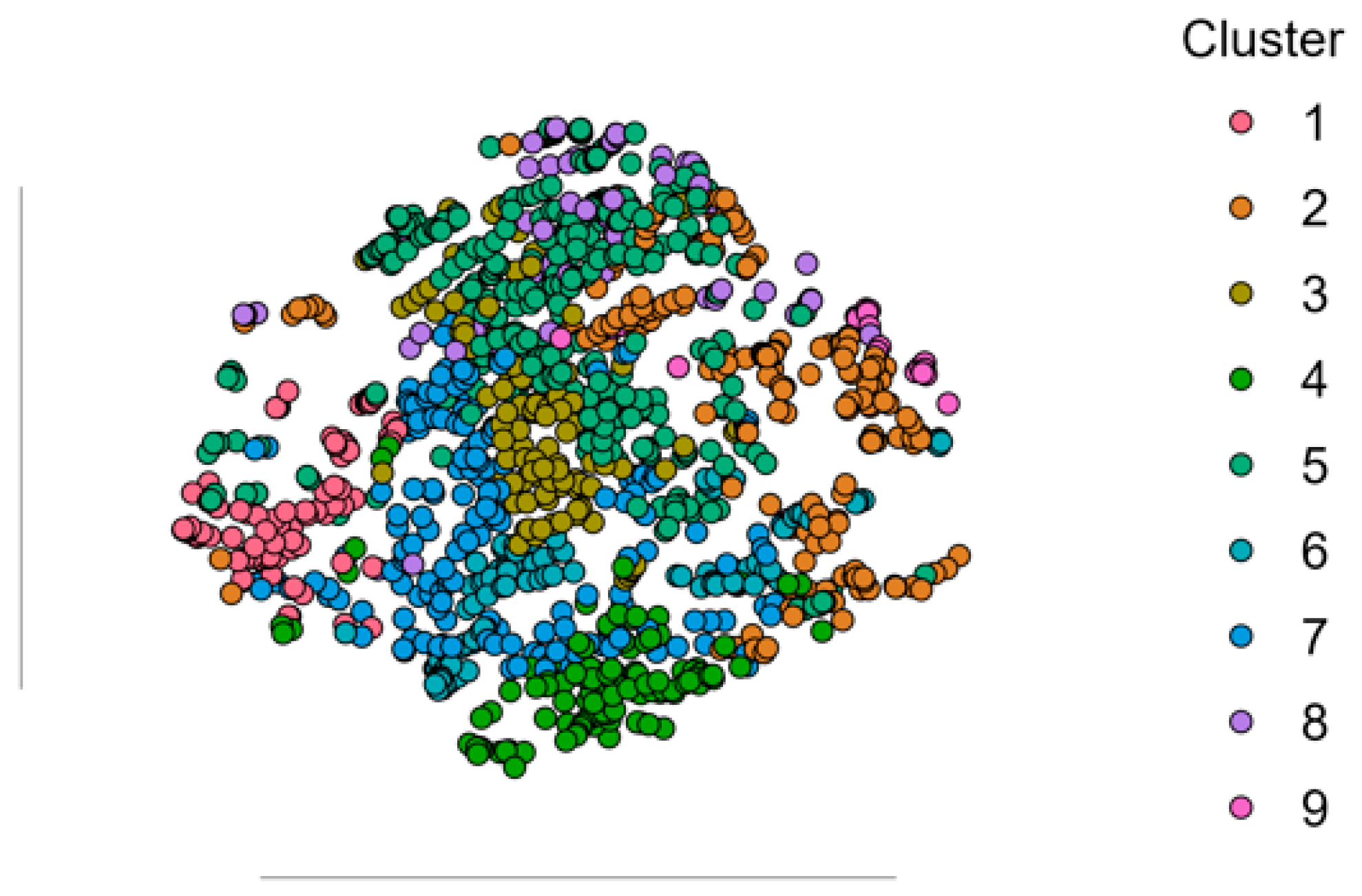
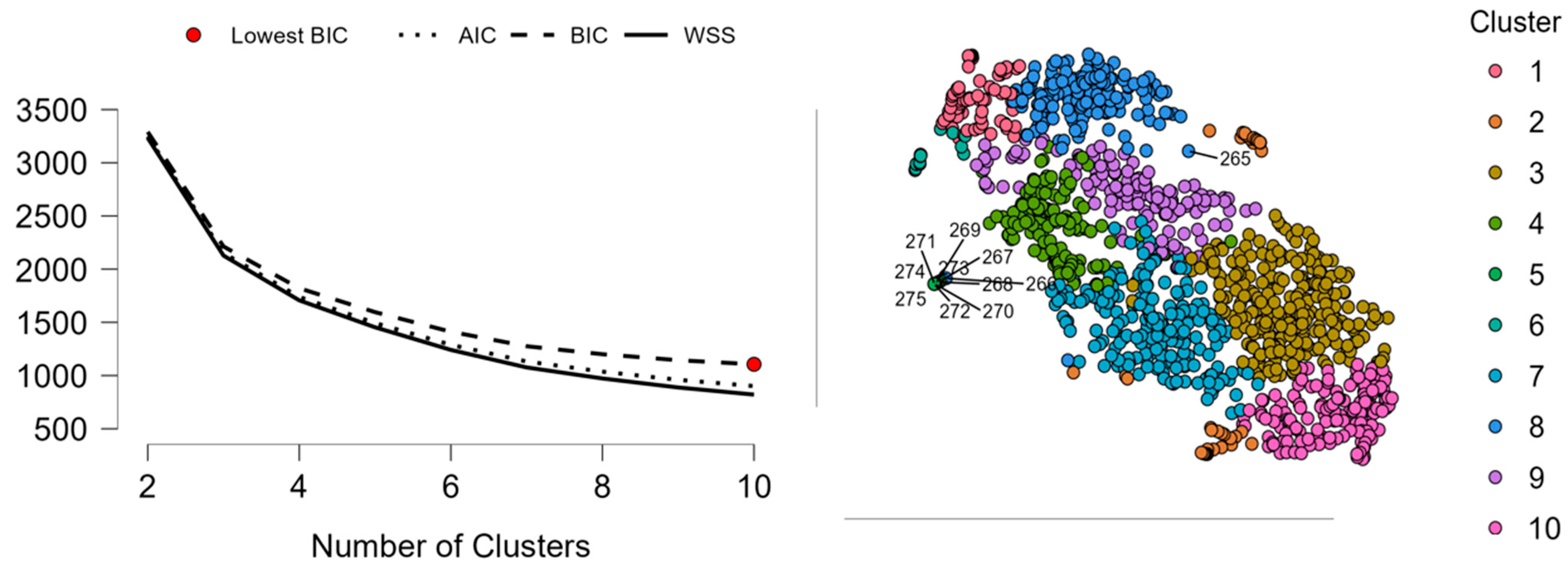
The figure displays the outcome of Fuzzy C-Means cluster analysis through a combination of statistical evaluation of the clustering model and visualization through cluster assignments inspection. On the left figure in the illustration, the model performance using cluster numbers two through ten is shown by taking the evaluation of the three important measures, namely, Within Sum of Squares (WSS), Akaike Information Criterion (AIC), and Bayesian Information Criterion (BIC). These measures direct the choice of the ideal number of clusters through a compromise between fit and model complexity. Due to heavier penalization against complexity than AIC, BIC plays a pivotal role in the choice between competing models. Here, the red marker point on the curve is put at the point where the corresponding solution is a nine-cluster value; this means nine clusters since it provides the best compromise between maintaining the structure of the data and overfitting the data. The declining WSS and flattening of BIC and AIC support this choice as it shows a sign of approaching the point where marginal improvement in the quality of the clustering in returning more than nine clusters will be extremely minimal. Having nine units thus remains statistically warranted and parsimonious compared to the complexity of the data (
Kaushal et al., 2024).
On the right-hand side of the figure, we have a two-dimensional visualization of the clustering result. The two-dimensional representation, presumably produced through the use of dimension reduction techniques such as t-SNE or PCA, diminishes high-dimensional data to a format permitting visual interpretation. Each marker marks a single record, and coloring illustrates cluster membership according to the Fuzzy C-Means function. The clustering appears typically coherent and dense aggregations of points and discrete color-coded sets of clusters occupy the plot area. There is undoubtedly some overlap—especially in the middle of the plot—due to the fuzzy approach to the method, where each and every marker will belong in part to two or more collections of clusters (
Shen et al., 2021). However, visual patterning assures success in segment capture by the function in the data. Large clusters labeled 2, 3, 4, and 6 dominate the visual area and correspond to the size range of the clusters the researcher had been working with earlier. Small cluster 8 and 9 cluster at the edge, and this will possibly reflect those occupying niche or specialist portions of the population.
On average, the image demonstrates good supportive evidence of the suitability of a nine-cluster solution for this analysis. Statistical assessment assures nine clusters offer the optimal compromise between model fit and model complexity, and the map illustrates the fact that the clusters are not just sensible but also are quite well-separated from each other (
Sunori et al., 2023). While potentially some fuzziness across boundaries is apparent—a typical concomitant feature of the Fuzzy C-Means algorithm—clusters are revealed with internal coherence and external differentiation. It validates the ability of the model to reveal complex and overlapping patterns in the dataset, and in the majority of real-world datasets, usually reflects a situation where categories do not tend to demarcate each other with sharp boundaries. The combination of the model diagnostics and visual inspection reflects the robustness and explanatory potential of the nine-cluster solution and renders it a good point of commencement for further interpretation, segmentation, or decision-making over the revealed groups (
Figure 2).
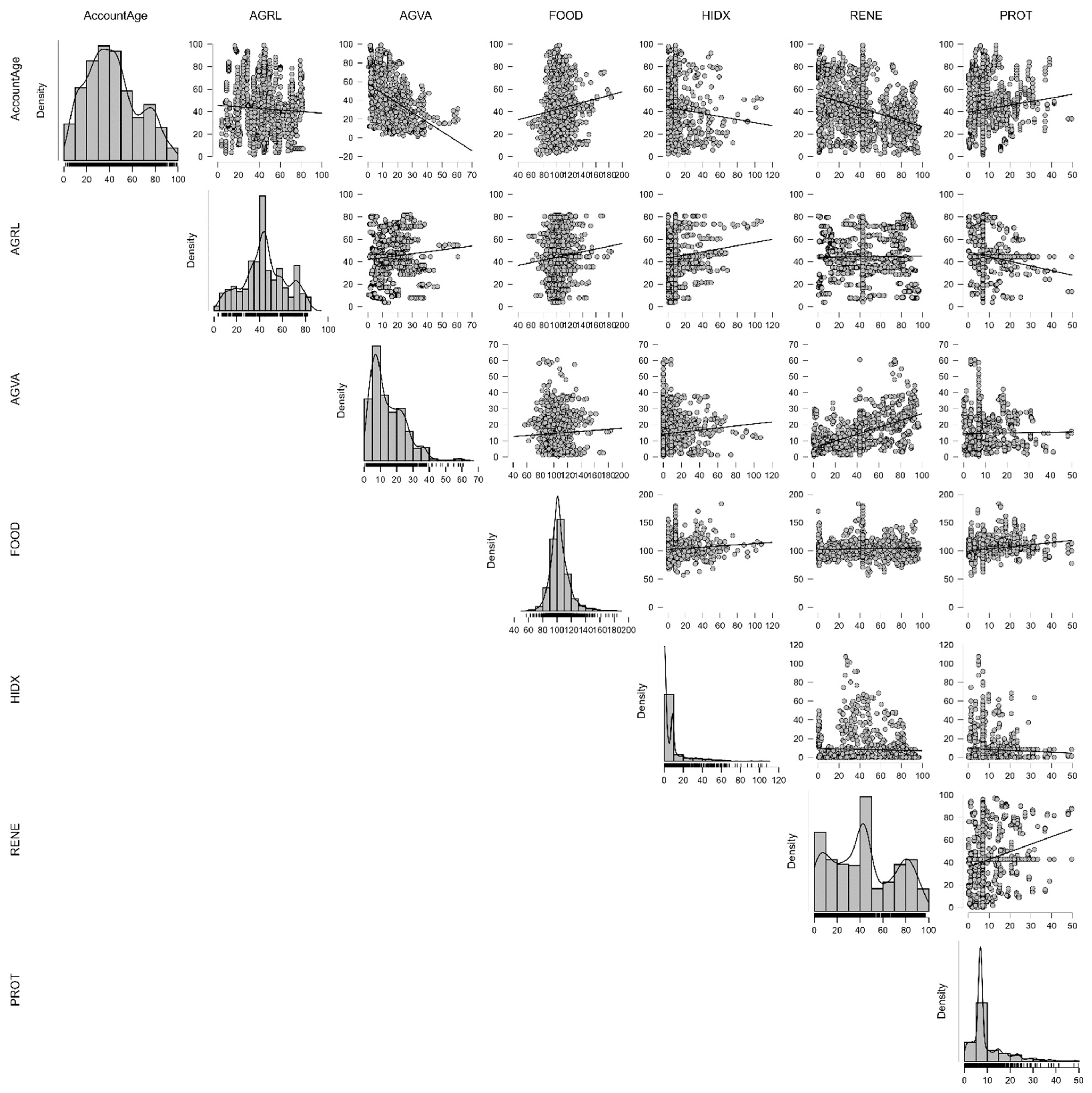
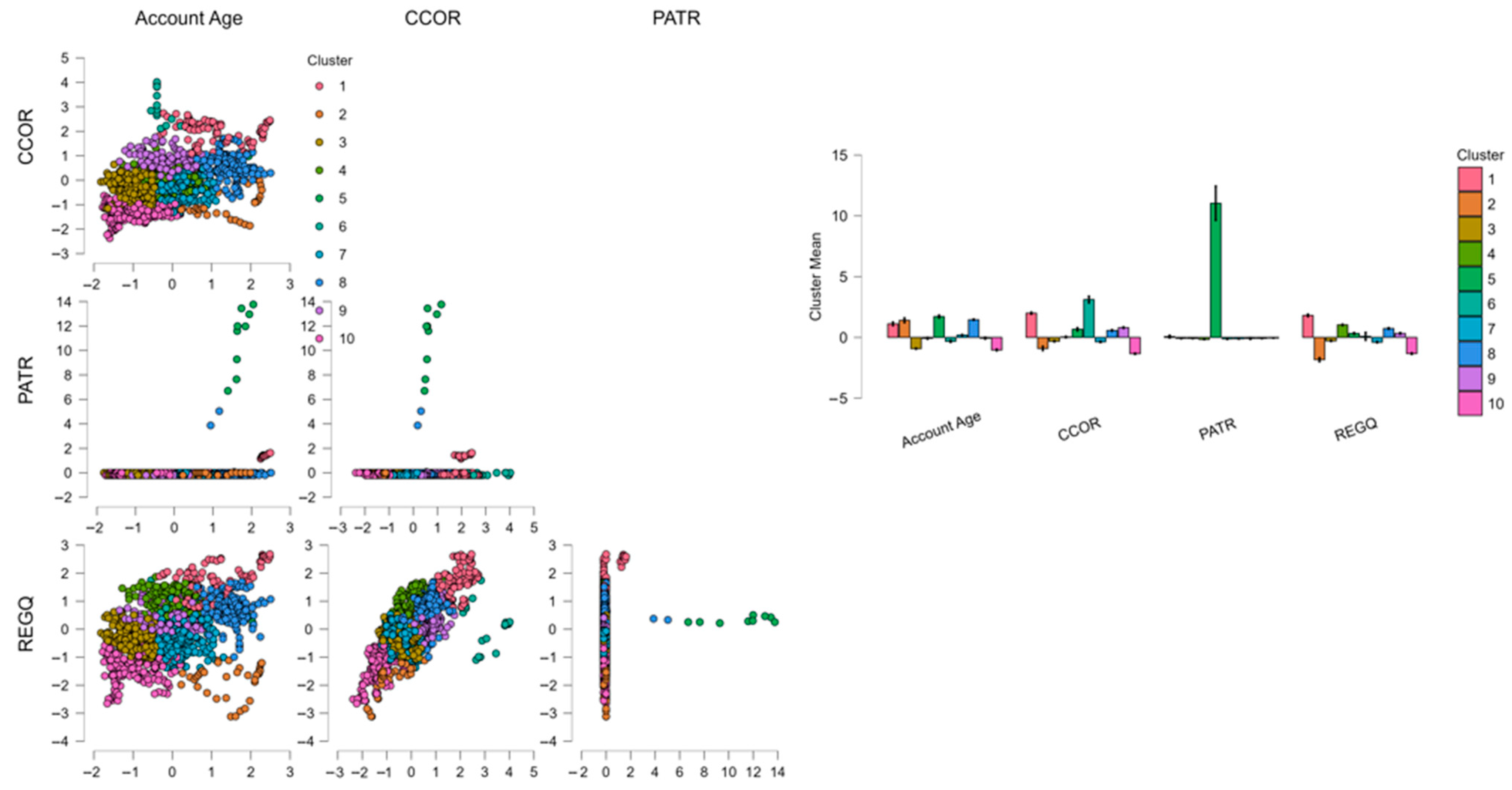
The figure displays a pairplot matrix examining the interaction between the level of financial inclusion as captured through Account Age—the proportion of individuals who own a bank account or a mobile money service—against a group of variables representative of the E (Environment) component of the ESG framework for developing economies. The included environmental variables used in the time series analysis were Agricultural Land (AGRL), Agriculture, Forestry, and Fishing Value Added (AGVA), Food Production Index (FOOD), Heat Index 35 (HIDX), Renewable Energy Consumption (RENE), and Terrestrial and Marine Protected Areas (PROT). The observations are color-coded by cluster membership from the Fuzzy C-Means clustering since each cluster defines a segment or profile of observations.
As part of this ESG framework emphasizing development, Account Age behaves as a surrogate measure of financial participation and access, essential elements of inclusive growth. A central question here is whether higher financial inclusion also correlates with better environmental performance or engagement. The distribution of Account Age is highly varied between clusters. Clusters 2, 4, and 9 show relatively high financial inclusion levels, and others like 6 and 8 cluster at the lower levels. These tendencies indicate that in developing nations, financial inclusion is not evenly spread and possibly correlated with dissimilar levels of environmental capacity and policy engagement (
Essel-Gaisey & Chiang, 2022).
Examining AGRL and AGVA in particular, which capture land use and economic productivity in agriculture—key sectors in many developing economies—higher Account Age clusters tend to have medium and high values. Illustratively, Cluster 4 has a high proportion of account holders and high agricultural participation. This could be taken as a reinforcing relationship: higher financial access may be generating agricultural productivity through loans, insurance coverage, and investments in technology, or vice versa, whereby higher productivity areas may be drawing better financial infrastructure (
Supartoyo, 2023).
The Food Production Index (FOOD) also offers added depth. Clusters 2 and 4 show a crossover between better financial inclusion and food production and thus could mean food security and access to finance complement each other. Conversely, both low FOOD values and low Account Age in Cluster 8 might reflect underserved areas having both production challenges and a lack of financial access, typical of more vulnerable segments in developing nations.
Renewable Energy Consumption (RENE) emerges as a very insightful variable. Cluster 9 stands out, having both a high score for renewable energy consumption and financial inclusion, which indicates a correlation between environmentally innovative policies or infrastructure and improved access to financial services (
Ababio et al., 2023). This trend confirms the assumption that green transition investment—e.g., off-grid solar or micro-financing for clean energy—may be concurrent with or promote financial inclusion.
PROT, a measure of the percentage of protected environmental areas, also displays a somewhat parallel trend. More affluent Account Age clusters like 4 and 6 also report above-average PROT levels, possibly as a result of policies at the local or national level combining financial access and environmental conservation efforts (
Said, 2024). In contrast, low-protection clusters like cluster 8 also report limited access to finance, supporting a trend of developmental weakness.
The function of HIDX (Heat Index 35), as an indicator of climatic stress, seems less specific, although cluster 1, which indicates high heat exposure, also has medium Account Age values. This could be a sign that a portion of the population experiencing climatic adversity may not always enjoy proportionate financial assistance and thus present equity concerns in climatic resilience planning.
As a whole, the pairplot verifies that financial inclusion—here measured through Account Age—crosses meaningfully with environmental variables at the heart of the E dimension of ESG. In developing nations, increased financial inclusion seems to co-occur alongside higher agricultural productivity, enhanced food security, the consumption of renewables, and the preservation of the environment. Conversely, areas of limited access to finance tend to coincide with economic and environmental deprivation. These findings reinstate the essence of aligning financial inclusion policy in the contexts of environmental sustainability policy, especially in emerging and under-resourced areas where ESG alignment presents both developmental and environmental returns on investment.
4.2. From Land to Finance: Machine Learning Insights on Environmental Determinants of Inclusion
We used eight regression models: Boosting Regression, Decision Tree Regression, K-Nearest Neighbors Regression, Linear Regression, Neural Network Regression, Random Forest Regression, Regularized Linear Regression, and Support Vector Machine Regression. These models were compared based on an extensive set of performance metrics: Mean Squared Error (MSE), Scaled MSE, Root Mean Squared Error (RMSE), Mean Absolute Error/Median Absolute Deviation (MAE/MAD), Mean Absolute Percentage Error (MAPE), and R
2 (coefficient of determination). To make the results comparable, results from all models were normalized based on Min-Max scaling, enabling us to map a 0–1 value range to each metric on all models (
Table 7).
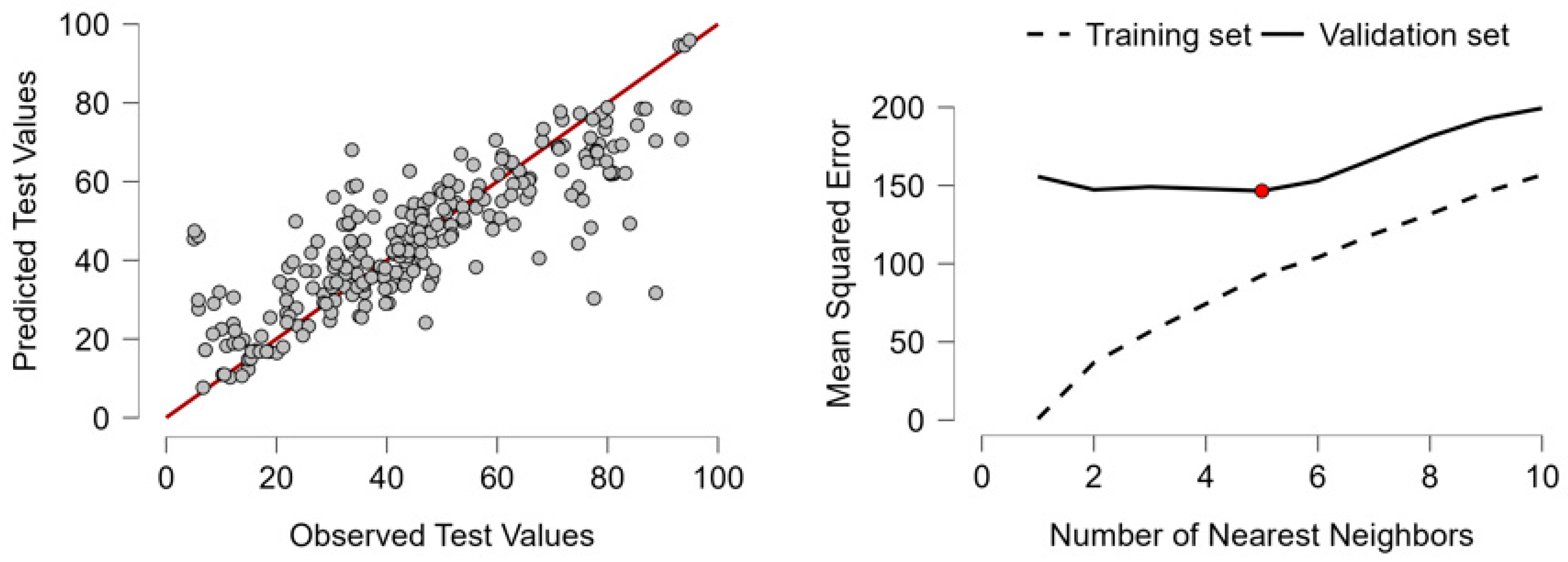
After normalization and aggregation of performance scores, Random Forest Regression came out on top as the best-performing model with a normalized average score of only 0.048, far below any other method. It also boasted the lowest MSE (162.916), lowest RMSE (12.764), and highest R2 (0.689), which clearly placed it as the best at explaining variance in financial inclusion on the basis of environmental predictors. Its performance stood far above conventional methods like Linear Regression (R2 = 0.226) or even sophisticated techniques like Neural Networks (R2 = 0.164), which, although possessing the theoretical advantage of being able to model non-linear patterns, did poorly on error scores.
These outcomes are theoretically in line with what would be expected from Random Forests. As a decision tree ensemble method based on bagging decision trees, Random Forest lends itself well to capturing non-linear, hierarchical, and interactive relationships between variables—properties found in environmental systems. The interaction between climate vulnerability (HIDX) and natural capital (AGRL, PROT), e.g., may be poorly captured through linear models. Likewise, the relationship between renewable energy take-up (RENE) and access to finance may be dependent on intervening conditions such as agricultural productivity or land use intensity, upon which a model like Random Forest can learn without specification in advance.
Furthermore, Random Forest has strong resistance against overfitting, particularly when compared to single decision trees or boosting models. This has a critical application in modeling environmental indicators between countries or regions that can differ significantly in size, resources endowed, as well as in institutional capacity. The capacity of the model in managing missing data, ranking feature importances, as well as the facility to accommodate noise, also makes it highly useful when dealing with imperfect real-world environmental data.
Conversely, other models in the comparison suffered from considerable weaknesses. As an example, K-Nearest Neighbors performed competitively on a few of the metrics but were sensitive to the presence of outliers and unsuited for the large environmental dimensionality. Boosting and Neural Networks, as strong performers generally, exhibited high error rates—likely as a result of overfitting or poorly optimized hyperparameters. Linear and Regularized Regression models, as easy-to-interpret models, performed poorly as a result of their failure to identify complex non-linearities inherent in the environmental space. The Support Vector Machine model also performed middling on all of the metrics and needs heavy tuning in order to perform at a peak level—less ideal for exploratory policy modeling.
From a policy and interpretability viewpoint, Random Forest also has other benefits. It allows for the estimation of the importance scores of features, giving insight into which environmental variables most significantly affect financial inclusion outcomes. As a case in point, initial model results indicate protected areas (PROT) and the consumption of renewably generated energy (RENE) carry high predictive weight, identifying the possible effect of conservation policy and green infrastructure on participation in the financial system. Such insight has particular utility in development planning, where the allocation of resources and environmental reform can be aligned with socio-economic inclusion on a strategic level.
The consequences of what we’ve found are significant. By showing that environmental factors can be used to predict financial inclusion at high levels of accuracy, and particularly when a Random Forest framework is used as the approach, we’re helping create a better-integrated view of sustainability. Financial inclusion is not simply a social or economic issue—it’s strongly rooted in the environmental situation of a country. In developing countries, where access to banks and the spread of mobile money increases at a very high rate, the environmental conditions of a region—whether it’s a high heatwave exposure, the take-up of renewable energy sources, or the degree of ecological preservation—will either facilitate or obstruct those changes.
Also, this research highlights the necessity of connecting ESG areas and not addressing them as disparate variables. The E component, so often dealt with as discrete from societal and governance institutions, here proves highly correlated with economic access and financial infrastructure. In the wider debate on sustainable growth, this finding lends credibility to the policy argument that efforts to make the environment more sustainable—such as conservation of resources or investments in green energy—ought not be merely regarded as climate actions but also as interventions having good spillovers in financial access and inclusion.
Ultimately, our thorough examination validates that Random Forest Regression is the most reliable and efficient approach for modeling the relationship between environmental variables and financial inclusivity in developing nations. Its theoretical flexibility, statistical performance, and empirical interpretability make it exceptionally suitable for ESG modeling, especially in rich data but structurally complex areas like the E component. As the worldwide community encourages enhanced, integrated, and fact-driven ESG disclosure, Random Forest presents a grounded and actionable solution path toward modeling and predicting environmental-socioeconomic linkages critical to ESG decision-making.
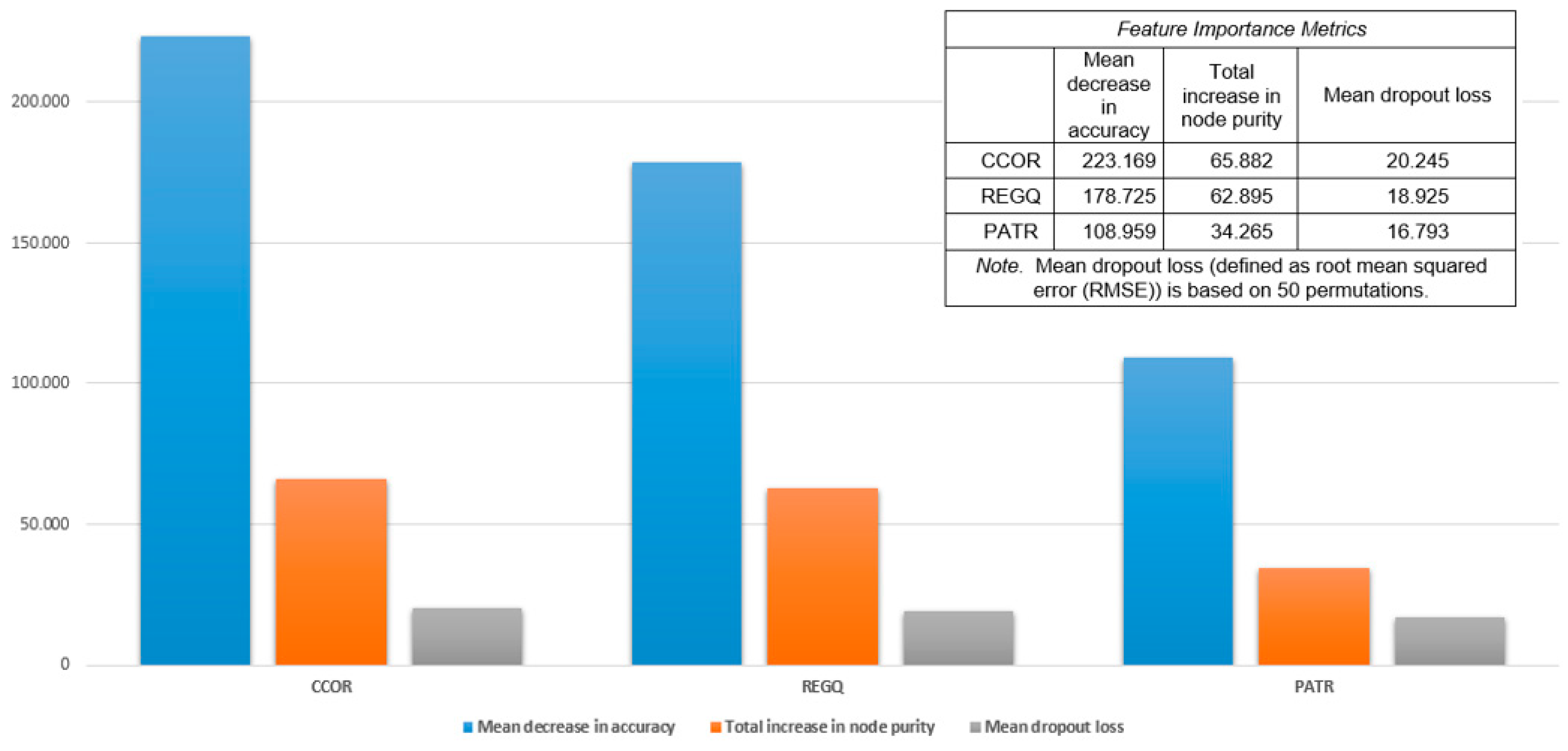
The application of Random Forest Regression as a means of explaining the link between environmental and financial inclusion, as reflected through the Account Age measure, offers insightful information on the interface between sustainability and financial access in developing economies. Account Age as a proportion of individuals who report having a financial institution or receiving money services in the last year can be taken as a good proxy for financial access. In this regard, a set of explanatory variables representing the most critical elements of the Environmental (E) pillar of the ESG approach was subjected to analysis. Such variables included Agricultural Land (AGRL), Agriculture, Forestry, and Fishing Value Added (AGVA), Food Production Index (FOOD), Heat Index 35 (HIDX), Renewable Energy Consumption (RENE), and Terrestrial and Marine Protected Areas (PROT). By explaining the impact of those environmental variables on financial access, the model provides a precise insight into development dynamics, bridging eco-resources and infrastructures, and socio-economic accessibility (
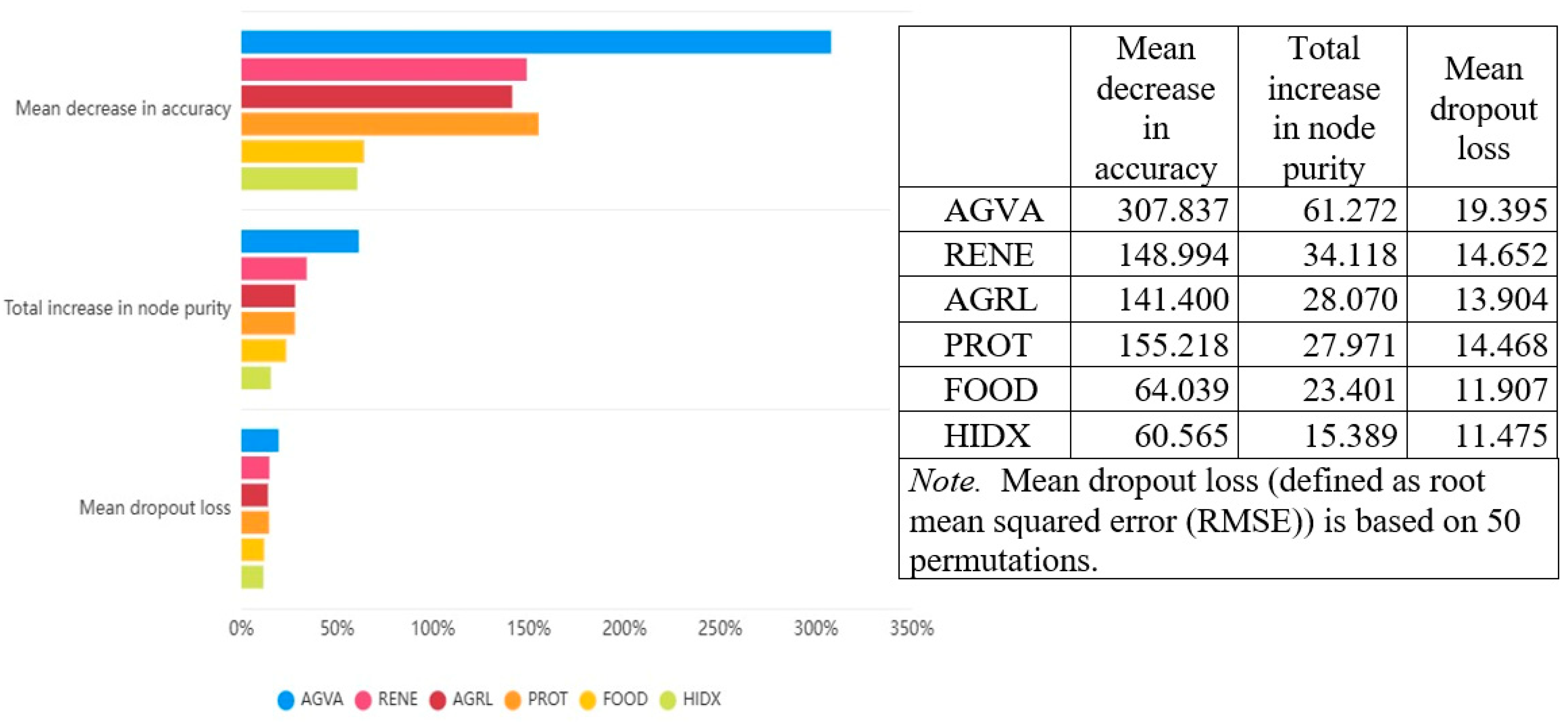
Figure 3).
Among the environmental predictors, the most important contributor to the predictive performance of the model came from AGVA. This was seen on all three importance metrics: mean reduction in accuracy, total boost in node purity, and mean dropout loss. The dominance of AGVA in the model indicates that areas of stronger economic production in the agriculture and agribusiness sectors experience increased levels of financial inclusion. The relationship may be explained by the fact that agricultural value chains tend to demand financial services like credit, savings, and insurance as well as production inputs and intermediation services, where smallholder farmers and local enterprises are involved and engaged in production for part or full cash payments. The relationship between economic production in agriculture and access to financial systems looks fairly strong and may indicate that investment in productive agriculture can simultaneously advance financial inclusion on a larger scale.
The second most powerful variable, renewable energy consumption, emphasizes the facilitating role of energy infrastructure in supporting financial participation. Renewable energy, and especially decentralized sources of it, such as wind and solar, have proven a key facilitator of digital finance and mobile money in areas without traditional access to electricity. Studies have shown that financial development and inclusion can significantly enhance renewable energy adoption, especially in developing countries (
Shahbaz et al., 2021). The framework’s identification of RENE as a key driver confirms the proposition that environmental sustainability and financial inclusion do not act at cross purposes and work best together. By making energy available, renewables indirectly facilitate the utilization of financial technologies and promote inclusive development (
Feng et al., 2022). Agricultural land, another critical predictor, points toward the role of land availability and utilization in determining economic conditions affecting financial behavior. Areas with larger agricultural land areas may enjoy higher involvement in agriculture and related industries, prompting interaction with financial institutions. Although less impactful than AGVA or RENE, AGRL’s significance indicates physical land resources continue to be central to development pathways, especially in agrarian economies. The performance of protected areas also deserves mention. PROT performed similarly to AGRL and RENE on the accuracy and dropout loss of the models. This might mean that environmental conservation policies may be linked to higher levels of financial inclusion, possibly due to stronger institutional arrangements or locally based approaches to natural resource management involving participation in formal systems. Or protected areas at higher levels may encourage sustainable investment or development financing, containing financial services as a part of wider socio-ecological resilience.
Food production index and heat index, although useful, were less impactful on the strength of the model’s predictions. FOOD, a measure of agricultural production, indicated modest significance, possibly because subsistence and food security may be supported by food production, but isn’t necessarily directly converted to financial participation unless linked to wider economic activity as captured in a more direct manner by AGVA. The lower significance of HIDX as a measurement of climate stress indicates that heat-associated impacts of the climate may be crucial for long-run sustainability, but less immediately impactful on financial participation. The implication here isn’t that climate variables don’t matter, but their impacts might be intermediated through other channels not captured in this model, e.g., migration, productivity losses, or effects on health.
As a whole, the Random Forest model has yielded a rich breakdown of the drivers of financial inclusion from an environmental perspective. Its capacity for dealing with non-linear relations and interaction between variables makes it well-suited for this form of multi-dimensional data, where relations between land use, climatic exposure, resource management, and economic activity involve complex interlinkages. The variable importance scores of the model give a clear indication of where environmental policy and financial inclusion policy may intersect. By pointing to AGVA, RENE, and PROT as the central levers, the analysis emphasizes sustainable environmental practices and efficient land use not only as critical for sustaining ecology but also as directly linked with access and empowerment related to finance. This aligns with emerging cross-country evidence that links renewable energy use and financial inclusion with inclusive growth outcomes (
Cui et al., 2022). This points toward the necessity for integrated policy responses, not viewing environmental sustainability and socio-economic inclusion as discrete agendas but as reinforcing aspects of development policy.
4.3. Forecasting Finance Through the Environment: A Case-Based Additive Explanation Approach
The “Base” value of 41.987 in every case indicates what the model’s expected prediction would be without any particular feature inputs included. The difference between the predicted value and the base would be the net effect of a positive or negative relationship each variable has on the final prediction.
For Case 1, the final forecast value (31.054) drops significantly below the base, largely due to huge negative contributions from AGVA (−7.839) and PROT (−3.647) dominating over positive contributions of RENE (+2.495) and HIDX (+0.401). It shows low agriculture value and little protected lands significantly depress predicted financial inclusion, even when renewably powered energy consumption has considerable levels (
Table 8).
Case 2 follows the same trend with a predicted value of 30.988—once much lower than the base level. AGVA also exerts a very strong negative impact (−8.530), and PROT has a negative effect (−4.185), but RENE has a positive effect (+2.732). These ongoing patterns reinforce the argument concerning levels of agricultural productivity and levels of protection determining the model and pulling projections down when levels are low, even when compensatory action from the consumption of renewable energy sources exists.
The Case 3 forecast for the model stands at 32.340, weighed down by AGVA (−8.462) as well as PROT (−4.156), but boosted by RENE (+2.718) and HIDX (+1.023). Significantly, in this instance, however, the FOOD variable enters a positive value (+0.120) for the first time and hence minimally alleviates the overall decline, suggesting some relief on the part of food production capacity in contributing toward upward momentum in projections of membership.
Case 4 presents a remarkably uncommon trend where the forecasted value (38.849) converges toward the base value. Although negative contributions from AGVA (−8.273) and AGRL (−2.461) persist, PROT strongly improves the forecast (+7.318), offsetting deficits. Case 4 illuminates the worth of protected areas as a potentially game-changer in the improvement of financial inclusion projections through signaling improved institutional arrangements or development assistance (
Figure 4).
Lastly, Case 5 has the strongest forecasting value (54.252), far above the base. The boost comes from high positive impacts from AGVA (+8.798), RENE (+5.772), and HIDX (+1.630), which dominate the small negative impacts from AGRL (−1.446) and PROT (−2.157). This case demonstrates the model’s ability to capture synergy between environmental and economic productivity, energy access, and good climatic conditions in improving financial inclusion outcomes.
On the whole, both instances identify AGVA and PROT as salient variables that tend to impose strong directional effects, negative when below average and positive when above average. The positive contributions from RENE consistently affirm the status of a key facilitator. The additive accounts well capture the ways in which sets of environmental variables determine the model’s outcome and provide clear insight into the mechanism by which environmental conditions impinge on financial inclusion in developing settings.
5. Social Foundations of Financial Inclusion: Empirical Evidence from Developing Economies
This research evaluates the effect of critical social variables on financial participation in developing countries on the “S” part of ESG. Literacy levels, educational attainment levels, internet penetration levels, labor market participation levels, life expectancy at birth levels, availability of sanitation facilities, and employment sex parity make up the proxy variables employed for financial participation in this research. Using both the G2SLS and TSLS models over a 12-year time panel, the study employs environmental instruments for addressing the challenge of endogeneity. The findings determine educational levels, internet coverage, good health levels, and employment sex equality as prominent drivers of financial participation and chart their usability for sustainable policy and development programs (
Table 9).
This empirical study sought to investigate the nexus between financial inclusion and the “S” (Social) pillar of the ESG framework, and developing countries specifically. Financial inclusion via the Account Age measure—calculated as the share of people who have a financial account or used a mobile money service in the preceding year—is a principal determinant for equal access to economic engagement and the formal financial system. In the ESG framework, the social pillar covers a subset of human development measures such as education level, health, gender equality, access to digital technologies, and labor participation. Such measures have a direct impact on people being able to use financial services and thus research the impact they have upon financial inclusion is both time and policy-oriented, especially in those countries where a significant proportion of the people are unbanked or underbanked (
Shahid & Asghar, 2024).
We examine this relationship through the use of a panel-data instrumental variable approach with both G2SLS random effects and TSLS fixed effects estimations. There are 1236 observations from 103 developing countries over 12 years. There are seven significant explanatory parameters all capturing the Social pillar of ESG: (1) Fertility rate (FERT), (2) Education expenditure through the government (EDUE), (3) Internet usage (NETU), (4) Labour force participation ratio (LABR), (5) Life expectancy at birth (LIFE), (6) Access to safely managed services and facilities to sanitation (SANS), and (7) Female-to-male labour force ratio (FLMR). These parameters capture the social infrastructure facilitating or limiting financial inclusion (
Jain et al., 2024).
The empirical findings based on both the G2SLS and the TSLS models are consistent and reinforce the evidence and validity of the findings to a great extent. In particular, the female-to-male labor force ratio (FLMR) is a positive determinant of financial inclusion and vindicates the role assigned to gender equality in sustainable development (
Wani & Khanday, 2024). Further, the use of the internet (NETU) is also the highest predictor of financial inclusion and verifies the role of the digital divide in economic participation (
Shahid & Asghar, 2024).
Government expenditure on education (EDUE) also shows a strong correlation with evidence referenced in research to highlight financial literacy and education as key enablers of access to services (
Zubair et al., 2023).
Finally, the approach aligns with the broader context of the integration of ESG factors, especially taking the socio-political complexities of policymaking towards sustainability in the Global South into account. Poor governance, misinformation, and ethics gaps can destabilize the financial system if left unresolved (
Alibašić, 2024).
5.1. Clustering Sustainability: Evaluating Algorithmic Performance on ESG-Environmental and Social Indicators
In the context of clustering algorithm evaluation on the E (Environmental) dimension of the ESG (Environmental, Social, Governance) framework, a comparison of five approaches—Random Forest Clustering, Neighborhood-Based Clustering, Model-Based Clustering, Hierarchical Clustering, and Fuzzy C-Means Clustering—was performed. The aim was to determine the superior-performing algorithm based on a set of normalization evaluation criteria: Maximum Diameter, Minimum Separation, Pearson’s γ, Dunn Index, Entropy, Calinski-Harabasz Index, R
2, AIC, BIC, and Silhouette. These evaluation criteria measure various aspects of clustering quality—compactness, separation, cohesion, and statistical fit of the model—and the evaluation was conducted based on the average of the normalized scores. The best-performing approach proved to be Hierarchical Clustering on average across the evaluation criteria used (
Table 10).
Hierarchical Clustering performed superbly on a variety of measurements. Specifically, it attained the highest possible score (1.0) on Minimum Separation, Pearson’s γ, Dunn Index, and Silhouette. This indicates very good clusters from a separation viewpoint, high internal correlation between clusters, an optimum intra- and inter-cluster dispersion ratio, and very good internal consistency. These are all key features when trying to make meaningful and interpretable distinctions between clusters, particularly in the case of environmental data where explicit groupings tend to reflect unique ecologies or policy regimes (
Rusu et al., 2023). The method also reported a relatively good Calinski-Harabasz Index (0.21), supporting the indication of structurally stable and statistically consistent clusters.
Hierarchical Clustering did not result in the optimum AIC or BIC values—both of which were established here at 0.0—but did provide a stable measure of R
2 at 0.44. This indicates a reasonably good variance-explaining ability. Such a compromise can be worthwhile when interpretability and cluster stability become more important than statistical optimum in and of itself. In sustainability and ESG applications, the ability to interpret and explain results in cluster analysis clearly will often be of more value than small gains in fit (
Saltık, 2024).
The second key strength of Hierarchical Clustering lies in the manner it presents the structure in visual form. The approach has the ability to create a dendrogram, a graph in the form of a tree representing the union progress and relationship between points or clusters visually. In ESG analysis—particularly environmental aspects—hierarchical visualization would be very helpful here (
Ishizaka et al., 2021). It not only gives the final cluster classification but also the constructive relationship between regions, countries, or observations. Its flexibility and clarity add a level of depth and may be used as a guide when making a decision on an optimum number of clusters based on policy or research at hand.
On the other hand, Random Forest Clustering, whose R2 (0.67) and AIC and BIC values were the best, fell behind on structural metrics such as Silhouette (0.43), Pearson’s γ (0.16), and Dunn Index (0.12). That means although it is statistically efficient, it may form less differentiated or compact groups, making interpretation and qualitative understanding less easy. Its predictive strength may be in being able to over-fit the patterns and hence reduce the reliability of capturing the true group structure.
The Neighborhood-Based Clustering emerged well on the Calinski-Harabasz Index (1.0) and on the Silhouette (1.0) as the best of the two, since it indicates well-defined clusters in some respects. It did poorly on Minimum Separation (0.10) and R2 (0.44) and functioned somewhat better on general interpretability-related functionalities than Hierarchical Clustering. It forms compact clusters, but a lower level of separation and explainability diminishes its usability in analysis where both statistical and policy relevance would be required.
Fuzzy C-Means Clustering attained the highest possible R2 value (1.0), thus theoretically highly capable of explaining variance. It failed on structure-related scores: Minimum Separation (0.0), Dunn Index (0.0), and Silhouette (0.57). While the soft clustering approach might be useful in those situations where observations truly belong to several categories, it can complicate the analysis when certain group labels must be established, particularly in policy settings where clear classification takes precedence.
The poorest performer on every measure was Model-Based Clustering, producing the lowest R2, Pearson’s γ, Dunn Index, Silhouette, and Calinski-Harabasz Index values. While model-based techniques give statistical rigor and probabilistic assumptions as their foundations, the results here portend failure on the part of the algorithm in extracting meaningful structure from the data. It has little interpretive insight and predictive utility, and so is a poor candidate for this ESG-focused analysis.
Briefly, the preference for Hierarchical Clustering is warranted by a balanced and stable performance on those ESG context-relevant metrics of chief concern: clarity, consistency, and structure. Its better performance in separation, internal cohesion, and visual interpretability harmonizes well with properties of environmental clustering, where complexity of data and policy decision-making call for models not just statistically sound but also interpretable from a stakeholders’ viewpoint (
Morelli et al., 2025). Hierarchical Clustering possesses a perfect balance between analytical accuracy and communicative capacity, which is essential in applications demanding clear and actionable information. Accordingly, it stands out as the best option from the algorithms evaluated as it offers the best possible tradeoff between statistical performance and usability in environmental ESG analysis (
Figure 5).
The Hierarchical Clustering output presents a meaningful division of the performance and shape of the model over the ten clusters found through the analysis. The sizes and consistency of the clusters differ, and their corresponding contributions toward explaining the variability in the dataset as a whole offer some interpretation over the extent to which the partitioning of data by the algorithm occurred in relation to group similarity and between-group spread.
The cluster group sizes vary from very small ones like Cluster 5 (11 units), Cluster 9 (5 units), and Cluster 10 (12 units) to very big ones like Cluster 2 (486 units) and Cluster 4 (279 units). It would not be abnormal if hierarchical models were of differing size because they cluster based on the merit of distance measurement and not size uniformity. Interestingly enough, the single cluster of Cluster 2 accounts for over 42% of the total of this within-cluster heterogeneity because it contains a big entry in the column on “explained proportion of within-cluster heterogeneity” (0.422). Similarly, Cluster 4 contains 25.6% of the within-cluster heterogeneity. These two clusters together explain most internal variability and may contain very diverse or loosely related observations, and possibly may call for a finer refinement or sub-clustering (
Table 11).
The WSS for size differences and heterogeneity reflects those differences as well. The largest cluster, Cluster 2, has by far the greatest WSS (1,888,726), reflecting the high internal variance of the cluster. The smallest clusters (e.g., Cluster 5, Cluster 9, Cluster 10) also hold very small WSS values, reflecting their small and compact aggregations of very comparable observations. The small clusters may be capturing niche or extreme profiles and could be very informative in the identification of outliers or high-interest groups, even if they capture a negligible amount of the dataset’s heterogeneity.
Silhouette scores give us another look at the quality of the clustering. By and large, the silhouette scores report a mixed story. Clusters 5, 8, 9, and 10 all contain very good scores (between 0.492 and 0.656), which means well-separated and internally homogeneous clusters. The single best-scoring cluster (0.656) is cluster 5, and this cluster also has the best internal cohesion and separation from other clusters in our measure. The two largest and most heterogeneous groups, Clusters 2 and 4, both contain the worst silhouette scores (0.066 and 0.067), which means they may contain overlap points from other clusters and urge us to be cautious in our interpretation. The fact that they both contain high internal variance and low silhouette scores means they may be aggregating heterogeneous or marginal points and would be better split or refined upon later analysis.
At a global level, the ratio between the sum of squares (BSS) and the total sum of squares (TSS) stands at 54.7. This makes about 54.7% of total variance explained through the clustering model—a very good percentage given the complexity and heterogeneity typically present in socio-environmental datasets. This reflects the goodness of the model in partitioning the data in a meaningful way, although adjustment will be necessary in the largest clusters.
Overall, the hierarchical clustering solution has an interpretable and well-balanced partitioning of the dataset. It well discovers small and well-separated clusters (e.g., Clusters 5, 8, 9, 10) and large general groupings (Clusters 2 and 4). The high silhouette scores of the smaller clusters attest to the appropriateness of the method in detecting niche patterns, and the explained variance (54.7%) validates good general performance. The findings justify the applicability of hierarchical clustering for ESG-environmental analyses where interpretability and discrimination between patterns are most critical. Further analytical procedures may entail re-clustering big clusters or applying other models so as to test and complement those results.
Cluster means. The clusters reveal evident patterns of correspondence between financial access as measured by Account Age and a set of concomitant social variables representing the S-Social column of the ESG framework in developing countries. Notably, Cluster 8 features the greatest standardized value of Account Age (2.046) and correlates highly with high life expectancies (LIFE = 1.339), social solidarity (SANS = 1.869), and female labor market participation (FLMR = 2.296). The implication here would be a clear positive correlation between financial access and social development, specifically institutional solidarity and gender participation. Conversely, Cluster 1 presents the lowest value of Account Age (−0.955) and encompasses lower education enrolment (EDUE = 0.438), labor market participation (LABR = −1.715), and female labor market participation (FLMR = 0.123), signifying a correspondence between poor societal institutions and lower financial access. Clusters 6 and 2 also reflect moderately positive Account Age values and couple them with sets of moderately positive labor dynamics and social solidarity, confirming multi-dimensional support as essential. At the opposite extreme, clusters 5, 7, 9, and 10 report negative values of Account Age as they record their respective levels of education (EDUE) and fertility (FERT), signifying the latter may not be an assurance of financial access without supporting socio-economic institutions. The complete set of patterns thus validates close interdependence between financial access and societal aspects, most importantly, gender participation, quality of life, and welfare provision, and calls once again for coordinated societal policies promoting inclusive financial ecosystems in developing countries (
Table 12).
5.2. Education, Equity, and the Economy: A Social ESG Perspective on Financial Participation
Of the eight algorithms under review—Boosting Regression, Decision Tree, K-Nearest Neighbors, Linear Regression, Neural Network, Random Forest, Regularized Linear Regression, and Support Vector Machine—the comparison of performance metrics on a uniform scale has a definitive winner. The comparison of the performance criteria is done using six standardized criteria: MSE, MSE (scaled), RMSE, MAE/MAD, MAPE, and R
2. These scores, when normalized, yield a common scale for comparison free from the variances brought about by differences in measurement units and magnitude (
Table 13).
K-Nearest Neighbors (KNN) is the top performer. It possesses the lowest values of MSE and RMSE at 0.00 each and also the lowest value of MAE at 0.00, figures which reflect little predictive error on the part of the algorithm. It also possesses the greatest R
2 value at 0.96 and hence accounts for nearly all the variance of the target variable. These figures firmly secure the top ranking in the rankings for this regression task on behalf of KNN. It would be a sign that the organization of the data suits well the instance-based and non-parametric nature of KNN, which excels at settings where locally salient patterns exist and are clearly defined (
Srisuradetchai & Suksrikran, 2024). All success notwithstanding, however, the weaknesses of KNN must be realized. It possesses weak scalability on higher datasets since it makes heavy reliance on lazy learning, and it’s highly sensitive to scaling and noise in features. Its performance on larger or dirtier datasets may be severely hampered unless pre-processing is extremely conscientious.
Boosting offers a good alternative. It does not lead on any single measure but scores well on all of them. Its normalized scores place it firmly in the middle or above, even at a modest tradeoff between variance and bias. At an R
2 of 0.53, it accounts for well over half the variance, a good showing considering the generally high variance-bias trade-off in ensemble algorithms. It also has an edge over KNN when it comes to complex data distributions via iterative error correction. This makes it generally better for real-world data, where data will be noisy and may well embody complex inter-relations between variables (
Ibarz et al., 2022).
Their performance here, however, is not as good as theory, and they perform poorly as well. The values here are very high in error, and they are particularly high in MAPE and MAE, and also indicative of high predictive imprecision. Their measure of R2 is also low and indicative of poor explanatory value as well. It indicates overfitting, or the data size and complexity of features are not sufficient for a neural architecture here. Without deep tuning and enormous data sets, their complexity here isn’t warranted.
Linear and regularized Linear Regression perform the worst here. Both share the assumptions of linearity and independence of predictors, both obviously violated here. Both models produce the largest error rates and lowest R
2 scores, and Linear Regression has a normalized R
2 of 0.00. These results indicate the limits of linear models when working with datasets having non-linear data or interactive complexities between variables (
Jin, 2022).
Decision Trees and Support Vector Machines also fall in between. Decision Trees perform erratically enough on a normalized MAPE of 0.00 (a probable normalization scale anomaly rather than performance), and an R2 of 0.11—which is far from adequate. Their overfitting tendencies are well established and here as well. Support Vector Machines fare a little better on consistency but do not perform well on any of the metrics and require very high computational resources without giving any superior accuracy.
From a generalizability and stability viewpoint, Boosting Regression could be better since it’s an ensemble method that smoothes out the variances between models. Nevertheless, from a strictly empirical viewpoint, the best on this dataset has been posted by the KNN, both in reducing each metric of error and optimizing explained variance on several performance metrics.
Overall, the top-performing model for this test is KNN. It beats out on key metrics and possesses high accuracy and explanatory power. If scalability, generalization, or immunity from noisy inputs were paramount concerns in a given situation, then a more adaptable and equally impressive solution option exists in the form of Boosting Regression. Currently, under these conditions and on these metrics, KNN stands as the statistically superior option.
In the context of modeling financial inclusion (Y), the K-Nearest Neighbors (KNN) algorithm outputs variable importance via mean dropout loss, which represents the increase in prediction error (specifically RMSE) when a given predictor is permuted or excluded from the model. This metric quantifies the marginal contribution of each variable to predictive accuracy, allowing for an assessment of their relative influence within the model’s structure (
Table 14).
From the S (Social) corner of the ESG (Environmental, Social, and Governance) framework and from the perspective of developing economies, evaluation based on the deployment using the K-Nearest Neighbors (KNN) model to estimate financial inclusion holds key implications (
Das & Nayak, 2020). Defined in this context as the share of the population who report holding a financial institution or mobile money account, financial inclusion is a core economic and social inclusion measure—a cornerstone of the ESG social pillar.
The result based on mean dropout loss—calculated as the mean increase in root mean squared error (RMSE) subsequent to each predictor variable being permuted in 50 simulations—provides a measure of the relative role played by the different socioeconomic variables in the determination of financial inclusion in low- and middle-income economies.
The largest variable is NETU (internet-using individuals), having the highest dropout loss at 18.755. This presupposes the key role played by digital access in facilitating financial inclusion in developing countries. Internet usage is more likely to serve as the starting point for digital bank services, cellular money apps, and other fintech services. The importance of the variable indicates the direction towards the improvement in social inclusion and access to finance (
Lee et al., 2023).
Next is SANS (access to safely managed sanitation services), with a dropout loss of 15.465. SANS is a structural quality-of-life and access-to-public-services measure. In developing countries, access to sanitation safety is related to urbanization, stages of development, and institutional coverage, and all are related to access to organized networks, including the financial system. SANS’ predictive power reflects the relation between economic inclusion and the infrastructure of basic public services.
The FERT (Fertility rate), measured as −15.351, provides a demographic background. Fertility is high in areas with lower education and access to medical care; conditions usually indicated through lower levels of financial inclusion. Fertility in this case acts as a proxy measure for overall conditions of human development (
Balde et al., 2022).
FLMR (female-to-male labor force) ratio decreases 15.312 and also holds a significant position in this regard. Inclusion of women in the labor force is hand in hand with financial inclusion: when women work, the probability of their maintaining bank accounts or utilizing financial instruments increases. This illustrates the significance of gender equality in the social part of ESG measurement.
LABR (Labor force participation rate), 14.863 in value, reflects the significance of overall economic activity. Access to the labor market—even insecure (informal) access to the labor market—encourages the use of financial services in the management of income, savings, and expenditure in developing economies.
On the lower rung in the list are the EDUE (Government expenditure on education) and the LIFE (Life expectancy at birth), both of which suffer losses to the tune of 14.447 and 13.670, respectively. Though they are significant gauges of people’s development in their own right, their implications with regard to financial inclusion can tend to be more lagged or indirect. The expenditure on education can impact financial literacy, but the tendency is towards a long-term rather than immediate effect. The life expectancy has more of a contextual rather than direct impact upon financial behaviour as a gauge of well-being in the community.
Overall, when looking at financial inclusion as the social ESG aspect in emerging economies, the findings clearly prioritize digital access, infrastructure fundamentals, and labor market participation—especially female participation. The highest-quality variables in terms of the highest loss in value are the categories suggesting structural and societal barriers to inclusion. Consistent with this logic, then are initiatives to promote internet penetration, the improvement in sanitation delivery, and women’s employment as high-impact interventions towards increasing financial inclusion and improving the social ESG ground in emerging economies
5.3. Forecasting Financial Access: Interpretable AI Insights from KNN in ESG-Social Contexts
The table presents additive descriptions of the financial inclusion forecasts calculated from the K-Nearest Neighbors (KNN) model utilized in the context of the Social (S) component of the ESG framework for developing countries. The goal variable utilized here defines financial inclusion as the percentage of individuals who own a financial account or make use of (mobile) money services. The forecasted value for every case has been provided from a base forecast of 42.032, and each feature then adds or detracts from it based on the strength of the effect (
Table 15).
For Case 1, the forecasted value of financial inclusion stands at 10.238, much below the base level. The decline here is mainly due to negative contributions from internet penetration, female-to-male labor force ratio, and government spending on education. These indicate poor access to digitalization, uneven employment opportunities between genders, and possibly wasteful spending on education as drivers of financial exclusion. Case 2 forecasts a value of 12.288 but remains well below the base level. High birth rates, weak internet penetration, and low spending on education contribute adversely once more, but a small positive effect from the female labor force entry ratio is observed. Case 3 has a forecasted value of 18.242, where negative contributions from a high birth rate are compensated for in part by positive contributions from life expectancy at birth, access to sanitation facilities, and participation of females in the labor force. The case indicates how enhanced basic infrastructure and gender equality can counteract negative effects from demographic stress (
Figure 6).
The predicted value rises in Case 4 to 31.890. Better sanitation access and a modestly positive fertility rate reinforce the prediction here despite adverse contributions from labor force participation and life expectancy. This indicates even when labor participation and health outcomes are less positive, good infrastructure in sanitation can remain a driving lever for financial inclusion. Case 5 experiences the greatest predicted financial inclusion at 36.722. This is driven primarily by high life expectancy and good internet use, and a positive fertility rate, but heavy negative contributions from expenditure on education and access to sanitation reveal possible inefficiencies or inequalities in the distribution of services. The extreme negative effect of education expenditure may indicate misalignment between expenditure and actual educational programs related to financial behavior. Generally speaking, the model results emphasize the stronger predictors of financial inclusion in the ESG’s social dimension as being internet access, fertility rates, and gender labor equity, alongside wider human development indicators such as sanitation and life expectancy. Whilst education has conventionally been regarded as a driver of financial participation, its repeated negative effect in these instances means investment itself will not be enough, and the quality and effectiveness of education programs must be the deciding factors. This points out the multi-sided nature of financial participation as guided not just by access directly to services but by the wider socio-economic context as well.
6. Governance Meets Inclusion: Empirical Insights from ESG Analysis in Developing Economies
This analysis looks at financial inclusion’s relationship with the “G” (Governance) pillar of the ESG framework in developing economies. As a financial inclusion measure, Account Age guides the analysis of its correlation with the three governance proxies: control of corruption (CCOR), patent activity (PATR), and regulatory quality (REGQ). Both G2SLS and TSLS models utilizing environmental instruments guide the analysis as it investigates whether access to financial services at a wider level fosters institutional development and accountability. The research confirms both opportunities—e.g., increased transparency and innovation—and challenges—e.g., potential regulatory loopholes—emphasizing the multifaceted dynamics between governance and financial inclusion (
Table 16).
This empirical study aims to explore the nexus of financial inclusion and the “G” (Governance) factor of the ESG (Environmental, Social, Governance) model in the context of developing countries. The principal assumption in our case is the fact that greater financial inclusion—measured through the Account Age variable, reflecting the proportion of the adult population with a bank account or using a mobile money service to make payments—might actually define the key governance performance measures. Financial inclusion is more than a financial marker: it is a force behind institutional growth and a citizens’ and governments’ accountability lever (
Zeqiraj et al., 2022). In this work, we are exploring whether more financially included societies are also more robust in their governance measures and specifically when focusing upon the control over corruption, regulatory quality, and innovation output respectively captured through variables CCOR, REGQ, and PATR.
As a counterfactual to account for concerns over endogeneity (e.g., since improved governance might also lead to greater financial inclusion), we apply an instrumental variables strategy using a G2SLS (Generalized Two-Stage Least Squares) random-effects and a TSLS (Two-Stage Least Squares) fixed-effects strategy using a panel dataset of 1236 observations from 103 developing economies over 12 years. Identification is achieved through a rich and carefully constructed set of environmental instruments—a methodological innovation spanning the environmental and the governance sides of the ESG framework (
Borgi et al., 2023).
Results from the two models both reflect statistically significant and economically significant relationships, albeit somewhat qualified in their implications. Most importantly, however, Control of Corruption (CCOR) is revealed to have a very strong and highly significant positive relationship with financial inclusion in the G2SLS and the TSLS models. This result verifies theoretical expectations and the literature: the greater the proportion of the population gravitates towards access to the formal financial system, the more difficult for the government to perpetuate corruption (
Ben Khelifa, 2023). Financial inclusion fosters transparency and traceability of activities and formal cashing out of transactions, both of which restrict the scope for instances of corrupt behavior.
The other institutional capacity and domestic innovation proxy, the second governance indicator, Residents’ Patent Applications (PATR), also exerts a positive and statistically significant impact on financial inclusion. Increasing financial inclusion should lead to enhanced innovation ecosystems—because greater access to funding enables more people and small firms to make research investments and engage in entrepreneurship activities (
Sanderson et al., 2018).
But the results for Regulatory Quality (REGQ) are more complex. While statistically significant, the coefficient is negative and shows that financial access extension can surpass institutional ability in the regulation of such services in some developing nations (
Kawor, 2023). This disconnect signals a key problem where fintech growth and penetration of mobile banking accelerate beyond the establishment of corresponding regulatory environments.
Overall, this study contributes to the research at the nexus of financial inclusion, governance, and sustainability. This study provides evidence of robust empirical support for a positive linkage between financial inclusion and both anti-corruption and innovation performance, and also identifies governance weaknesses concerning regulatory quality. The incorporation of green instruments in the estimation furthermore firmly supports causal inference and is consistent with the ESG logic of systemic interdependence.
6.1. Clustering Governance: Evaluating Algorithmic Performance on ESG-G Data
The comparison of clustering algorithms—Fuzzy C-Means, Hierarchical, Model-Based, Neighborhood Based, and Random Forest—across the normalized performance criteria gives a holistic view of their relative performance in the unsupervised classification task. The evaluation parameters used here comprise R
2, AIC, BIC, silhouette score, maximum diameter, minimum separation, Pearson’s γ, Dunn index, and the Calinski-Harabasz index. All the criteria have been min-max normalized between 0 and 1 so that comparisons can be made directly between them. The aim here is to identify the best-performing algorithm in general in the aspects of cluster quality, cohesion, separation, and interpretability (
Table 17).
From R
2, which indicates the extent of the clustering structure explaining the variance in the data, Neighborhood Based has a perfect 1.0, showing high explanatory value. Hierarchical comes next at a good 0.73 rating, and the rest lag behind and score only 0.0—meaning little or no clustering structure is present. This already pushes Neighborhood Based and Hierarchical approaches ahead since variance explanation has a lot of relevance as a measure of clustering quality when clusters are anticipated to capture clear-cut informative groupings (
Blasilli et al., 2024).
The Akaike Information Criterion (AIC) is generally applied to measure model parsimony, and lower values are desirable. As AIC has been inversely normalised, Neighborhood Based has a clear 1.0 value representing the optimum fit for complexity. The remainder of the models record a value of 0.0 and therefore perform apparently less well in relation to the simplicity of the model versus fit. This must be taken as read, however, as AIC proves very lenient on complex models if they’re not compared against other measures of separation. The Bayesian Information Criterion (BIC) offers a stronger penalty on complexity than AIC. In this case, the Model-Based method has the best performance (0.82), showing good explanatory strength without overtraining, followed by Fuzzy C-Means (0.75) (
Ambarsari et al., 2023). Neighborhood Based, although doing well at AIC, has a score of 0.0 at BIC, which may indicate that it has an excessive complexity when measured through a stricter penalty framework. Random Forest has a perfect 1.0 here, in a seeming contradiction, although this may be the effect of the normalization scale rather than true interpretability, especially since it fares poorly at other scores (
Sarmas et al., 2024).
Silhouette score, which indicates the similarity of an object to its own cluster versus other clusters, benefits the Neighborhood Based approach again at a top score of 1.0 once more. Hierarchical also scores well at 0.9 and suggests well-separated and well-clustered groups. Fuzzy C-Means (0.49) and Model Based (0.21) lag behind, and Random Forest (0.0) falls at the bottom once more. Since the silhouette score directly relates cluster cohesion and cluster separation, the findings strongly affirm the consistency of Neighborhood Based and Hierarchical approaches (
Putra & Abdulloh, 2024).
With respect to Maximum Diameter, smaller scores describe more dense clusters. Hierarchical clustering has the best (0.0), with very dense cluster formations, and Fuzzy C-Means (1.0) and Random Forest (0.98) making the loosest clusters. Model-Based and Neighborhood-Based take a middle ground, although compactness will not be enough on its own in order to measure clustering quality since extreme dispersion, as in Fuzzy C-Means and Random Forest, usually goes together with poorly defined clusters (
Azkeskin & Aladağ, 2025).
On the other hand, Minimum Separation—a larger value corresponding to a larger inter-cluster distance—is greatest in Hierarchical clustering (1.0), reflecting superior discrimination, followed by Random Forest (0.14) and Neighborhood Based (0.08). Fuzzy C-Means (0.02) and Model-Based (0.0) indicate extreme cluster overlap. This confirms Hierarchical clustering’s performance in creating clear groupings, a key requirement for explainability in applications such as customer segmentation or ESG scoring.
The Pearson’s γ between cluster assignments and true distances is maximum for Hierarchical clustering (1.0), yet another reflection of the clarity of its structure. Neighborhood Based (0.45) and Random Forest (0.37) also perform well in terms of structure, although Fuzzy C-Means and Model-Based perform very little. It seems, therefore, that Hierarchical clustering has the best preservation of the natural order of the data in the partitioning. The intersection of compactness and separation occurs at the peak of the Dunn index (1.0), validating its ability to produce dense and well-separated clusters. Neighborhood-based has a minimal value (0.11), and all other models approach zero, demonstrating poor trade-offs between intra-cluster cohesion and inter-cluster separation (
Vikrant & Bhattacharjee, 2024).
Entropy, conventionally utilized as a measure of the uniformity of cluster distribution (lower being preferred), has here a reverse sense: high values denote increased disorderliness. Neighborhood Based (1.0) and Fuzzy C-Means (0.98) both share the greatest entropy and hence irregular cluster size or mixed distribution of classes, unwanted in most application contexts. Hierarchical has the lowest entropy (0.0), as expected from a method having a proclivity for producing purer and evenly split clusters. Finally, the Calinski-Harabasz index, which favors clusters having high between-cluster dispersion and minimum intra-cluster variance, strongly favors Neighborhood Based (1.0), followed by Hierarchical (0.39). Fuzzy C-Means (0.04) and the rest lag behind, with Random Forest also scoring 0.0. This final measure reiterates the perception that Neighborhood Based performs best in forming statistically stable and well-defined clusters.
Summing over all aspects, the Neighborhood Based method always ranks at or close to the best in the most important criteria: R2, AIC, silhouette score, and Calinski-Harabasz index. Nevertheless, a low BIC and high entropy indicate possible overfit or cluster size imbalance risk. The Hierarchical method presents a good alternative as a stable approach, ranking highly in silhouette, minimum separation, Pearson’s γ, Dunn index, and entropy—attributes leading to well-defined and interpretable clusters with preserved structure. Model-Based and Fuzzy C-Means clustering algorithms show some single-point strengths, like good BIC (Model-Based) or entropy alignment (Fuzzy), without consistently performing well on the entire set of measurement techniques. Random Forest emerges as the worst clustering approach in this situation and performs poorly in almost all categories except a good BIC score, which itself is not enough to counteract the poor performance on silhouette, R2, and Calinski-Harabasz index.
Finally, Neighborhood Based clustering proves the best performer in general on this dataset and evaluation approach. Its superiority in multiple key measurements renders it the ideal solution for realizing significant patterns from highly internally coherent and well-separated data. Hierarchical clustering comes in as a close runner-up, producing better-balanced and interpretable clusters and being well placed for applications demanding clear hierarchical organization and small-cluster size. Depending on application necessity—whether prioritizing precision, simplicity, or interpretability—one or the other may be the best solution, and Neighborhood Based is preferred when performance on the model is the top priority, and Hierarchical when clarity of structure matters most.
The Neighborhood clustering results present a differentiated interpretation of financial inclusion in developing nations from the Governance (G) component of the ESG framework. The estimation of financial inclusion (measured through Account Age) employs the Control of Corruption (CCOR), Patent Applications by Residents (PATR), and Regulatory Quality (REGQ) as the three key governance predictors. The clustering analysis sheds light on governance-related profiles correlated with enhanced or reduced levels of financial inclusion in various settings (
Table 18).
Ten clusters were detected, each corresponding to a unique governance-financial inclusion profile. The cluster size ranges surprisingly from as few as 9 observations (Cluster 5) to as many as 260 (Cluster 3), reflecting varied distributions of governance features in the data. Explained proportion of within-cluster heterogeneity and within sum of squares (WSS) measure compactness; lower WSS and higher explained proportions tend to reflect well-coherent clusters. As an example, small but statistically significant (34) Cluster 2 has a relatively modest WSS (37.137) and high silhouette score (0.350), reflecting well-defined internal consistency. The largest cluster in the sense of explained within-cluster heterogeneity (0.174) has a good silhouette score (0.380), reflecting it as both cohesive and differentiated from surrounding clusters (Cluster 8). The cluster silhouette scores between 0.248 (Cluster 7) and 0.694 (Cluster 5) also measure cluster quality. The highest silhouette score accompanies Cluster 5, which denotes unique distinguishability from other clusters and indicates high uniqueness in governance-financial inclusion tendencies. In contrast, although having a sizeable share (212), Cluster 7 has a rather low silhouette score of 0.248 and indicates overlapping with adjacent clusters or intra-cluster heterogeneity. These insights are consistent with recent findings highlighting the power of clustering in revealing latent structure in financial and governance data (
Bester & Rosman, 2024); (
Bhaskaran, 2023). Examining the cluster centers of Account Age, we can start deciphering the relationship between governance characteristics and financial inclusion. Clusters at positive Account Age centers—e.g., Clusters 1 (1.116), 2 (1.409), 5 (1.717), 8 (1.457)—reflect higher levels of financial inclusion. These are especially interesting when combined with good governance scores. Cluster 1 has high financial inclusion coupled with good governance indexes (CCOR = 1.994, REGQ = 1.812), reflecting a situation where low corruption and good regulatory quality facilitate access to financial institutions. Cluster 5, although small in size, has the highest Account Age center (1.717) and very high patent applications (PATR = 11.038), possibly a sign of a subgroup more innovative and economically active and thus possesses good institutional features (CCOR = 0.670, REGQ = 0.328). On the other hand, negative Account Age centers—most notably Clusters 3 (−0.925), 4 (−0.073), 10 (−1.036)—indicate lower financial inclusion. Cluster 10 stands out as most noteworthy: not only has it the lowest center for Account Age but also highly negative governance scores (CCOR = −1.344, REGQ = −1.333), which are consistent with a framework of poor institutions, low trust levels, and poor regulation and thus probable obstacles to financial inclusion. Likewise, Cluster 2 indicates strong financial inclusion coupled with negative governance scores (CCOR = −0.911, REGQ = −1.834), a counterintuitive finding which may indicate local policies or local financial arrangements independent of governance quality (
Майoрoва et al., 2023). Another interesting example is Cluster 6, with the greatest CCOR score (3.114) and a mildly negative Account Age center (−0.326). Although possessing superior corruption control, financial inclusion here is not as robust—presumably because other missing elements of the necessary structures, e.g., education or access to the digital platform, are not reflected here, given the governance-centric approach of the model. The activity of PATR in clusters tends to be subdued generally, as a majority of clusters reveal near-zero or negative standardized values, and only Cluster 5 appears as a clear outlier here. This indicates that patent activity might not be a robust direct driver of financial inclusion in most instances, although the dominance of Cluster 5 suggests a niche where innovation and financial access may be correlated (
Figure 7).
Taken as a whole, the clusters capture the multi-dimensional nature of the governance-financial access relationship. Strong governance—regulatory quality and anti-corruption—tends usually to be associated with increased levels of financial access, but not in a purely linear relationship: There are clusters (e.g., Cluster 2) featuring relatively high levels of financial access coupled with weak governance, suggesting the role of non-commercial systems, NGO activity, or local variation in institutional performance. From a policy point of view, Neighborhood Based clustering method indicates strategic clusters in which governance reforms would pay the greatest dividends in terms of financial inclusion. Moderate governance and low inclusion clusters (e.g., Cluster 4) can be strengthened through specific financial infrastructure improvements. High innovation and good governance, and access clusters (e.g., 5) would be indicated as exemplars of good practice demonstrating the synergy of institutional strength and economic dynamism. Thus, the Neighborhood Based clustering approach has successfully distinguished governance-financial inclusion profiles in developing nations. It points out both regular patterns—e.g., the positive effect of regulatory quality—along with outliers—e.g., high-inclusion clusters in the face of poor governance. These results not only hold academic interest but also assist in the design of interventions for increasing the societal impact of governance reform in the ESG framework.
The Neighborhood Based clustering gives a useful overview of the interplay between governance variables and financial inclusion in developing economies. The aim of the analysis is the estimation of financial inclusion—defined as Account Age, or the availability of access to institutions or mobile money accounts—according to three governance variables: Control of Corruption (CCOR), Patent Applications by Residents (PATR), and Regulatory Quality (REGQ). The clustering creates ten profiles in the dataset differentiated by their average values (mean) in the four variables (
Table 19).
At the beginning, the mean Account Age also varies extensively by cluster from a high of 1.717 for Cluster 5 to a low of −1.036 for Cluster 10. The standardized values indicate differences in financial access or utilization. High cluster values for Account Age might be understood as reflecting populations with increased access or participation in formal financial institutions, and lower values reflecting lower financial access or utilization (
M. Ahmad et al., 2022).
Cluster 5 is a telling example. It possesses not only the largest Account Age (1.717), but also a very high patent application value (PATR = 11.038). Both of them suggest an ecosystem dominated by innovation and financial engagement. The governance indices on this profile, namely, the CCOR (0.670) and the REGQ (0.328), are fairly positive, i.e., the quality of governance is good but not excellent. This profile would define a niche of nascent innovation economies where good-quality governance coexists with high creative productivity and good-quality financial facilities (
Kaplan et al., 2024).
The lowest Account Age at −1.036 also comes from cluster 10 and the worst governance scores: −1.344 for CCOR and −1.333 for REGQ. These reflect a pervasive corruption and weak regulatory capacity context. The negative PATR at −0.046 here also suggests minimal innovation activity. This cluster would likely be for failing or fragile governance regimes where both institutional trust and innovation would be low, and therefore where financial inclusion would be confronted strongly by obstacles (
Zeqiraj et al., 2022).
Cluster 1 also features high financial inclusivity (1.116 Account Age) underpinned by high levels of CCOR (1.994) and REGQ (1.812), and a low level of PATR (0.066). This cluster would then capture a good governance and stable context featuring acceptable levels of innovation and good regulatory quality. This configuration aligns with development models in which institutions’ strength has a direct impact on financial integration (
Acheampong & Said, 2024).
Cluster 2, on the other hand, has a contradictory narrative as well. It has negative governance scores—CCOR at −0.911 and REGQ at −1.834—but the second highest Account Age at 1.409. It may be the case that financial inclusion can progress regardless of—or even despite—bad governance in some contexts. It may be because of the impacts of non-governmental financial systems, e.g., microfinance or mobile money platforms, which may be able to persist even in low levels of institutional quality. Or this cluster may be demonstrating states in transition where legacy infrastructure continues to provide financial access as governance drives through chaos (
Jungo et al., 2022).
Cluster 8 presents another performing scenario when it comes to financial inclusion (Account Age = 1.457), coupled with good governance scores: CCOR (0.573) and REGQ (0.736). The low and negative PATR score of −0.085 merely suggests a scenario where a stable and well-regulated system provides financial services even without high levels of innovation. This validates the hypothesis that regulatory quality plays a central role in achieving financial inclusion through the removal of entry and operation obstacles, consumer protection, and fostering competitive financial sectors.
Clusters 3 and 4 offer middle-ground examples. Cluster 3 offers low Account Age (−0.925), poor governance (CCOR = −0.318, REGQ = −0.287), and minimal patent activity. The cluster likely contains contexts of stagnation where both governance and innovation are lacking and thus diminish financial access. Cluster 4 offers a nearly neutral Account Age (−0.073) and a moderately positive REGQ (1.033), which suggests formal strength in regulation may not be enough to stimulate financial inclusion in the absence of trust in governance or innovation. This adds strength to the contention that regulatory systems must be positioned effectively and supplemented by other system strengths if they are to be impactful on inclusion (
Figure 8).
Cluster 6 stands out through a very high level of CCOR (3.114), the highest in the sample, and a negative Account Age (−0.326). Although having a highly controlled corruption, low financial inclusion indicates that controlling corruption by itself may not be enough to promote access to the financial system (
Zeqiraj et al., 2022). Since the moderate REGQ (0.088) and low PATR (−0.116) both show a lack of regulatory movement and innovative economic activity, the cluster may be indicative of post-reform settings in which corruption has already been tamed but other institutional or economic development has not caught up yet.
Cluster 7 has average scores on all indices (Account Age = 0.190, CCOR = −0.367, and REGQ = −0.394) and depicts a middle-to-low level of governance and limited financial intermediation. The countries in this cluster must be at a nascent phase of their institutional reform or be unevenly developed in sectors (
Ben Khelifa, 2023).
Cluster 9, which has a near-zero Account Age of −0.063, weakly positive governance (CCOR = 0.805 and REGQ = 0.334), and little innovation activity, is another interesting case in point. It has fairly good governance scores, but not necessarily corresponding financial inclusion strength. This might mean governance effects take time to show themselves in concrete socio-economic means such as financial access or possibly other forces—such as financial literacy, infrastructure, or cultural attitudes—intervening as inhibitors (
Okereke et al., 2023).
Throughout the clusters, certain patterns emerge. Strong governance scores tend to be associated generally with higher financial inclusion, as in Clusters 1 and 8. This would be in line with the ESG approach’s assumption that good governance is the bedrock upon which inclusive economic systems operate. Secondly, outliers such as Clusters 2 and 6 contradict this story and indicate that financial inclusion may take place even in low-governance environments or be non-existent even in high-governance ones. These aberrations illustrate the governance-inclusion relationship’s complexity and the necessity of mediating variables such as technology, education, and the financial systems present in the informal sectors.
Thirdly, innovation activity (PATR) seems to be a less significant determinant. Except in cluster 5, which has very high innovation and corresponds also to the most financial inclusion, in all other clusters, PATR stays close to or even below zero. This means innovation can be a catalyst for financial systems, but it is not a panacea in governance in the sense of inclusivity.
Finally, the Neighborhood Based approach effectively pinpoints the complexity of developing country governance-financial inclusion dynamics. It not only indicates anticipated correlation patterns but also key exceptions in between, providing a data-driven platform for policy interventions aimed at specific areas of action. Its implication for policymakers is that governance has to be enhanced indeed, but complemented by efforts in infrastructure development, financial education, and rollout of technology. This multi-dimensional understanding harmonizes well with the ESG worldview, where governance is a standalone measurement but a supporting pillar for wider development objectives.
6.2. Predicting Inclusion: A Machine Learning Benchmark on Governance Predictors
The performance of regression algorithms must be evaluated in a multi-dimensional manner, balancing both error minimization and explanatory strength. Eight algorithms (Boosting Regression, Decision Tree Regression, K-Nearest Neighbors (KNN) Regression, Linear Regression, Neural Networks, Random Forest, Regularized Linear Regression, and Support Vector Machine (SVM)) are compared here on a set of six normalized performance scores: Mean Squared Error (MSE), Scaled MSE, Root Mean Squared Error (RMSE), Mean Absolute Error (MAE/MAD), Mean Absolute Percentage Error (MAPE), and the coefficient of determination (R
2). All performance scores are minmax-normalized on the scale 0–1 so they can be directly compared, where smaller values for error scores (MSE, RMSE, MAE, and MAPE) denote better performance and larger values for R
2 indicate better model fit (
Table 20).
The first model to consider would be Random Forest since it performs almost perfectly across all measures of error: MSE (0.0), RMSE (0.0), MAE (0.0), and scaled MSE (0.0). It also registers the highest achievable R
2 (1.0), since it captures the entire variance of the dependent variable (
Du et al., 2022). The relatively low value of MAPE (0.14) indicates this model strikes a good accuracy vs. generalizability balance. The zeroes placed in the error measures on a scaled space mean that out of the models considered, Random Forest registered the lowest raw errors. Pairing this with the highest R
2, a strong case would be made for Random Forest to emerge as the highest-performing model in this assessment (
H. Zhang et al., 2020).
Following close behind is also K-Nearest Neighbors Regression (KNN), also with excellent performance in a normalized MSE (0.05), RMSE (0.06), MAE (0.09), and scaled MSE (0.0), all measuring minimal error in predictions. KNN also gets a perfect R2 value of 1.0, indicative of excellent explanatory ability. Its slightly higher MAPE score of 0.09 versus 0.14 from Random Forest indicates slightly improved performance in percent error. Although KNN does have excellent performance, however, it is sensitive to noisy data and computationally ineffective in big datasets, and so potentially limited in real-world applications. Nevertheless, based strictly upon performance in terms of results, the close similarity between KNN and Random Forest means the slight trade-off in interpretability and scalability might be worth it with small or cleansed datasets.
Boosting Regression ranks third and also performs well on MSE (0.12), RMSE (0.13), MAE (0.17), and MAPE (0.0), all excellent performance metrics. The high point to note is that it also returns the high R
2 value of 1.0. The extremely low MAPE value of 0.0 might reflect very accurate computation of percentage error, and Boosting Regression can be very beneficial where proportion errors play a big role, say in finance or marketing. The extremely low figure of error against other domains in comparison with Random Forest and KNN means that while Boosting can be very potent, it might not be as consistent with broader performance metrics (
Chauhan, 2024).
Decision Tree Regression performs poorly in all the measures: MSE (0.5), RMSE (0.52), MAE (0.59), and scaled MSE (0.45) indicate significantly higher levels of error relative to the top three models. Its R2 value (0.52) also talks about poor explanatory ability in explaining less than half the variation within the data. The MAPE (0.58) is also higher and reflects lower reliability in making percent predictions. The interpretability and simplicity of the Decision Tree are well-documented, but this overfitting and sensitivity over varied datasets can be observed from the above result.
Linear Regression, being simple to interpret and conceptually in character, performs poorly across all the measures. Its error levels are average: MSE (0.31), RMSE (0.34), MAE (0.46), and scaled MSE (0.77). Its R2 value is just 0.20, reflecting the fact that it can explain very little variance in the data. While the MAPE is respectable (0.15), showing improved proportion forecasting, as a performance measure overall, it shows that linear regression doesn’t have the ability to understand the complexity in the relation between the variables in the data.
Regularized Linear Regression also seeks to improve the general linear model in its aim to reduce overfitting but provides inconsistent predictions. While the MSE value (0.48) and the RMSE value (0.51) are better than those of the Decision Trees, both its MAE value (0.67) and the MAPE value (0.53) are high. Its R2 value (0.3) beats the R2 value of Linear Regression, but lags behind the rest of the non-linear algorithms. This shows that while the use of regularization improves the linear model, it cannot entirely compensate for the flaws in the linear model in its ability to capture the complex patterns in the dataset.
Support Vector Machine Regression performs the worst in several key areas. It produces extremely high normalized MSE (0.78), RMSE (0.8), MAE (0.79), and worst MAPE (1.0) for purposes of percent error, and measures very low R2 (0.14), implying low explanatory value. SVMs do potentially become very strong if a suitable kernel and tuning are employed, but their extremely high complexity and sensitivity to their parameters likely stop them from doing very well here.
In the bottom position in the performance rankings is Neural Networks, worst-ranked across all the important measures of error: MSE (1.0), RMSE (1.0), MAE (1.0), scaled MSE (1.0), and worst-after-the-second MAPE (0.65). Its R2 (0.0) further means they have no predictive ability whatsoever. Even though they are very valuable in complex, higher-order problems, poor performance here shows as overfitting, weak training, or network-incompatibility with the data set. Their need for large data sets and computing brawn drains their utility here as well.
Out of all the eight algorithms, Random Forest is the highest performer with the minimum errors and highest model fit (R2 = 1.0), the highest degree of generalizability and reliability across a range of applications. Its ensemble property gives it the ability to define complex patterns without overfitting, a theoretical requirement in real predictive use cases. KNN performance is similar but can result in lower scalability and more demanding data preprocessing needs. While very accurate in relative error, Boosting does have slightly higher absolute error and may be susceptible to overfitting if left tuned improperly.
Mid-range models like Regression and Decision Trees are somewhat useful in terms of interpretability and convenience but are weak in performance. SVM and Neural Networks also don’t do too well, and this illustrates the wisdom in the selection of a model based not only on theoretical potency but also empirical fit to the available data and context.
Lastly, based on this multi-metric ranking, the Random Forest is the best general-purpose regression predictor for predicting financial inclusion or similar socio-economic indicators in this sample. It displays the best combination of predictive accuracy, low error, and explanatory power, and thereby emerges as a general-purpose machine learner suitably suited to many different sorts of regression predictions.
The initial algorithm to look at would be Random Forest, as it has nearly perfect performance on all error measures: MSE (0.0), RMSE (0.0), MAE (0.0), and scaled MSE (0.0). It also has the best possible R
2 (1.0), as it accounts for the full variance of the dependent variable. The modest value of MAPE (0.14) suggests this model has a good balance between accuracy and generalizability. These findings are consistent with studies such as those by
Remegio (
2024), who demonstrated the efficacy of Random Forest in predicting student performance with impressive results (
Remegio, 2024), and
Sood et al. (
2023), who showed its predictive strength in real estate analytics during COVID-19 (
Sood et al., 2023).
Coming close behind it is K-Nearest Neighbors Regression (KNN), which also has stellar performance, with minimal prediction error and a perfect R
2 of 1.0.
Teguh et al. (
2024) confirmed this effectiveness when applying KNN in environmental data classification alongside Random Forest, noting its reliability when working with clean datasets (
Teguh et al., 2024).
Boosting Regression also scores high, especially in scenarios where proportional errors are significant. Meanwhile, Decision Tree Regression and Linear Regression perform moderately to poorly across several metrics. These conclusions are echoed in the comparative evaluations by
Kaliappan et al. (
2021), who tested various regression models on COVID-19 reproduction data and found ensemble methods like Random Forest to significantly outperform linear models (
Kaliappan et al., 2021).
Interestingly, while Support Vector Machines (SVM) and Neural Networks have theoretical strengths, their performance in this evaluation was weak, reinforcing findings from sports analytics by
Sanjaykumar et al. (
2024), where Random Forest clearly outperformed other models in predicting outcomes in cricket matches (
Sanjaykumar et al., 2024).
Ultimately, this evaluation confirms that Random Forest offers the best balance of predictive accuracy, minimal error, and model robustness across a wide range of applications, aligning with the most recent literature (
Figure 9).
The data below depicts the application of a Random Forest Regression to estimate financial inclusion in developing nations. The target variable employed here is Account Age, defined as the proportion of individuals having a financial institution account or using mobile money accounts. It will act as a proxy for financial inclusion—a key driver for socioeconomic development and a pillar of the Social (S) part of the ESG framework. Yet in this model, we will be estimating financial inclusion based on variables representing the Governance (G) part of ESG: Control of Corruption (CCOR), Patent Applications by Residents (PATR), and Regulatory Quality (REGQ) (
Table 21).
The case’s predicted value is then moved from the base by the additive effect of CCOR, PATR, and REGQ. The additive accounts allow us to view the effect of a change in each of the governance variables on the estimation of financial inclusion and thus provide insight into each of the governance components’ relative effect on financial accessibility. The forecast value in Case 1 is 26.780, which falls below the base level significantly. The fall here is dominated by extremely negative contributions from both REGQ (−7.309) and CCOR (−7.830), and a lesser effect from PATR (−0.471). The magnitude of the effects suggests financial inclusion gets heavily repressed in the contexts where both corruption levels and regulatory quality are high. The result is not surprising: higher corruption levels tend to destroy trust and deter financial formalization in both government and the finance sector, and poor-quality regulatory institutions impose disincentives on access to finance. The minor effect of patent applications here suggests innovation itself cannot act as a proxy for poor institutions in promoting financial inclusion (
Figure 10).
Case 2 shows a much closer estimate to the base (40.801) under mixed governance contributions. Here, both CCOR (−5.596) and PATR (−0.915) remain negative but less intense than Case 1 and are almost offset by a strong positive effect from REGQ (+4.923). This trend suggests that even if corruption persists as a challenge, good governance has a compensatory effect whereby it permits access to a greater number of financial services through regulated channels (
Ben Khelifa, 2023). The example: well-regulated mobile money services, consumer protection regulations, or easy financial onboarding may drive inclusion even in contexts where trust in institutions remains low.
Case 3 has a forecasted Account Age value above the baseline (45.063), thanks mainly to a very large positive contributor from PATR (+7.373). Both CCOR (−4.189) and REGQ (−0.511) happen to be small and negative but not very significant quantitatively. This indicates a unique set of conditions where innovation—through fintech, digital platforms, or entrepreneurial ecosystems—bridges financial exclusion despite governance frailties (
Okereke et al., 2023). In developing nations, private-sector innovations in financial tech have opened alternative channels of inclusion irrespective of, or even in the face of, government ineffectiveness.
Case 4’s even stronger forecast (45.580) benefits from a high REGQ effect (+5.348) and positive PATR (+1.221), and a modest drag from CCOR (−3.379). This input set illustrates synergy between good regulatory conditions and modest innovation in supporting financial access. If institutions can establish inclusive financial policies—e.g., identity checks as a requirement for access, e-banking systems, or financial education drives—conditions become ripe for large-scale financial participation (
Zeqiraj et al., 2022).
Case 5 also has a similar profile to Case 4 and features a projected value (44.243) above the base as well. The positive contributions from REGQ (+2.644) and PATR (+2.469) and the negative impact of CCOR (−3.260) reinforce the previous conclusion: regulatory capacity and innovation together form a formidable force behind financial inclusion and may neutralize the adverse impact of corruption to some extent.
Across all cases, the Control of Corruption (CCOR) variable shows a consistent negative impact on financial inclusion, supporting the argument that corruption has a systematic role in reducing access. It deters participation in the formal system, induces institutional mistrust, and marginalizes vulnerable groups. On the other hand, Regulatory Quality (REGQ) plays a largely positive role, providing a supportive environment for inclusion via financial service rules, consumer protections, and outreach incentives. Patent applications (PATR), while impactful in some cases like Case 3, do not substitute for institutional strength and are most effective when paired with solid governance.
Overall, this Random Forest Regression illustrates that in developing countries, financial inclusion is strongly influenced by governance characteristics, where anti-corruption, regulatory quality, and innovation must work in tandem.


