Abstract
Zimbabwe’s economy has experienced extreme exchange rate fluctuations over the past decades, driven by persistent macroeconomic instability and episodes of hyperinflation. The instability in exchange rates can significantly impact trade balances, inflation rates, and overall economic resilience. Understanding the impact of exchange rate volatility (ERV) on international trade is crucial in such a context. This study investigates the impact of exchange rate volatility (ERV) on international trade in Zimbabwe, addressing a literature gap related to its unique economic challenges and hyperinflation. Using the Generalized Autoregressive Conditional Heteroscedasticity (GARCH) model on data from 1990 to 2023, the study finds a negative relationship between ERV and international trade. The analysis suggests that inflation reduces imports, but foreign direct investment (FDI) and balance of payments (BOP) increase export uncertainties. This study recommends optimal fiscal and monetary management to mitigate ERV and enhance trade stability, offering insights for policymakers to strengthen Zimbabwe’s trade resilience amid exchange rate fluctuations.
1. Introduction
International trade is crucial for the growth of open economies, facilitating access to diverse goods and services that enhance productivity and innovation (Baldwin, 2016). It also strengthens international relationships, promoting cooperation and stability (Rodrik, 2021). A stable exchange rate is essential for global competitiveness; however, the shift to flexible exchange rates post-Bretton Woods has introduced challenges, such as exchange rate volatility driven by capital flows and speculation (Gopinath, 2020). The exchange rate represents the value of one currency relative to another. It is determined by the demand and supply of foreign currency in the market, along with the expectations and confidence of economic participants. Various factors can influence the exchange rate, including inflation, interest rates, fiscal and monetary policies, external shocks, and political instability. Exchange rate volatility refers to the degree of fluctuation in the exchange rate over time. It indicates the uncertainty and risk linked to changes in the exchange rate. The effects of exchange rate volatility on trade can be both positive and negative, depending on the nature and extent of the fluctuations, as well as the characteristics and reactions of traders.
Zimbabwe is a landlocked nation in Southern Africa that has encountered numerous economic and political difficulties since 1980. A significant issue has been the instability of its exchange rate, which has impacted its trade performance and overall competitiveness. Zimbabwe has faced significant exchange rate fluctuations due to hyperinflation and currency reforms, disrupting its international trade and creating uncertainty. For instance, the collapse of the Zimbabwean dollar led to a drop in export earnings from USD 26 billion in 1997 to USD 1.3 billion by 2006 (Hanke & Kwok, 2009). Traditional theories suggest a negative relationship between exchange rate volatility and trade, with increased risks discouraging cross-border transactions (McKenzie, 1999). However, findings vary, especially for developing nations where instability can disproportionately affect economies reliant on imports (Choudhri & Hakura, 2006). They emphasize that higher inflation environments intensify the impact of exchange rate movements on domestic prices. Developing countries often exhibit greater Exchange Rate Pass-Through (ERPT) due to weaker institutions and less credible monetary policies, which can lead to a feedback loop of inflation and currency depreciation. This vulnerability is compounded by dependence on imported essentials like food and energy, making these economies especially sensitive to external shocks such as geopolitical tensions and supply disruptions (Amaglobeli et al., 2022). Overall, the literature highlights the critical need for tailored policy approaches to mitigate ERPT effects in developing economies.
Below in Figure 1 is a trend analysis of exchange rate fluctuations and their effects on imports and exports in Zimbabwe during the dollarization, multicurrency, and post-multicurrency system.

Figure 1.
Zimbabwe exchange rate, import, and export indicators.
During the early 2000s, Zimbabwe’s hyperinflation peaked at an estimated 89.7 sextillion percent in November 2008, prompting the introduction of multiple currencies (Hanke & Kwok, 2009). By 2009, the economy dollarized, which stabilized imports but saw exports decline from 42.30% of GDP in 2009 to 37.59% in 2015 (Kanyenze et al., 2017). Despite dollarization, export competitiveness did not improve significantly. From 2016 to 2018, a multicurrency system led to notable fluctuations, with imports rising from 19.94% to 26.16%, while exports fell from 31.28% to 28.39% (Zimbabwe National Statistics Agency (ZIMSTAT), 2018). Between 2019 and 2023, the introduction of the RTGS currency resulted in steep depreciation and increased import levels from 26.16% in 2018 to 27.96% in 2022, before decreasing to 22.5% in 2023 (World Bank, 2023). This volatility disrupted trade performance, complicating pricing and delivery for exporters and increasing costs for importers.
Theoretical models such as the risk aversion and sunk cost model suggest that exchange rate volatility negatively affects trade, as factors like risk aversion, hedging constraints, and sunk costs discourage international transactions. However, empirical findings are mixed. Ilzetzki et al. (2023) observe a strong negative impact on trade in developing nations, while Broll and Lockwood (2001) report weaker effects in advanced economies with better risk management. Studies by Choudhri and Hakura (2006) and Gopinath (2020) show that the impact varies with factors like financial development and trade openness. Although theory supports a generally negative relationship, the effects depend on economic conditions and development levels. This study focuses on Zimbabwe’s unique economic challenges, exploring how exchange rate volatility influences trade while addressing inflation and foreign direct investment, areas previously underexplored (Berg & Borensztein, 2000).
Problem Statement
Over the past two decades, Zimbabwe has experienced persistent exchange rate instability, hyperinflation, currency reforms, and the adoption of multiple currencies (Mhaka, 2019). This volatility has severely impacted trade performance, with exporters struggling to maintain consistent pricing and delivery schedules, thereby hindering their global competitiveness. Importers also face substantial challenges in managing costs and maintaining profitability, especially those dependent on imported raw materials, machinery, or finished goods (Mpofu, 2019). The uncertainty surrounding exchange rates forces firms to adjust pricing strategies, often resulting in higher consumer prices and reduced affordability of imported goods. Additionally, the instability of Zimbabwe’s currency complicates long-term planning and investment decisions, increasing the risk of international trade transactions and deterring potential foreign investors, which hinders overall trade and economic growth (Chikwature & Chidhagu, 2016). Therefore, this study seeks to investigate the effects of exchange rate volatility on Zimbabwe’s international trade, aiming to assist policymakers and business leaders in developing strategies to alleviate these risks and enhance trade competitiveness. According to the research goals, this study aims to analyze the impact of exchange rate volatility on trade in Zimbabwe, specifically assessing how fluctuations in exchange rates influence the country’s exports and imports. Key objectives include evaluating the direct effects of exchange rate volatility on Zimbabwe’s trade activities, determining the relationship between inflation (INF), foreign direct investment (FDI), and international trade, and exploring strategies that Zimbabwean businesses can implement to mitigate risks associated with volatile exchange rates. Understanding these dynamics is crucial for policymakers and businesses in Zimbabwe as they navigate the challenges posed by exchange rate instability and develop effective risk-management technique.
2. Literature Review
The relationship between exchange rate volatility (ERV) and international trade is underpinned by several theoretical frameworks, some of which are less applicable to developing economies. Traditional theories, such as risk aversion and hedging limitations, suggest that increased ERV raises uncertainty and transaction costs, discouraging trade (Dornbusch, 1980). However, theories like the portfolio balance model and real options framework may not hold in the context of developing nations due to their limited access to financial instruments (Ameziane & Benyacoub, 2022). For instance, Ethier (1973) argues that firms can benefit from volatility if they can hedge against risks, yet many developing economies lack the financial markets necessary for effective hedging, making this theory less relevant. Consequently, the lack of risk management tools in countries like Zimbabwe exacerbates the negative impacts of ERV on trade.
Empirical evidence on the effects of ERV on trade varies significantly between developed and developing economies. Studies have shown that developed nations, with their advanced financial systems, can better absorb the shocks associated with exchange rate fluctuations, thereby mitigating adverse effects on trade (Blanchard, 2010). In contrast, developing economies often experience heightened vulnerabilities due to factors such as limited access to capital markets and weaker institutional frameworks (Peree & Steinherr, 1989). Research focusing on developing economies indicates that while ERV can disrupt trade, the evidence remains sparse, particularly for nations like Zimbabwe, where economic instability compounds the challenges faced (Choudhri & Hakura, 2006; Mlambo & Moyo, 2020). This gap in the literature highlights the need for further investigation into the specific impacts of ERV on trade in Zimbabwe’s unique economic context.
While Chimhore and Chivasa (2021) examined Zimbabwe’s exports to South Africa during the stable multicurrency regime (2009–2016), our study extends the literature by analyzing ERV’s impact on both imports and exports across Zimbabwe’s hyperinflationary (pre-2009) and post-dollarization (2016–2023) periods. Crucially, our GARCH framework captures volatility effects that OLS (used in prior work) overlooks, revealing three key divergences tied to Zimbabwe’s economic structure:
Institutional Fragility vs. Stable Trading Partners
Unlike Chimhore & Chivasa’s finding of weak ERV significance (10%) in a stable regime, our results show ERV is strongly negative (1% significance) amid Zimbabwe’s currency crises, highlighting how institutional instability (e.g., lack of hedging tools) amplifies trade risks.
Dependence on Imports
Zimbabwe’s reliance on imported essentials (e.g., fuel, machinery) makes inflation-driven ERV (coefficient: −0.005) more detrimental than in diversified economies (e.g., Nyunt’s 2019 ASEAN study found positive ERV effects).
Regional Trade Bloc Dynamics
While prior studies (e.g., Mosbei et al., 2021 on EAC) show ERV’s neutral impact in dollarized regions, Zimbabwe’s partial dollarization post-2016 failed to mitigate ERV’s trade drag due to monetary policy inconsistencies—a nuance absent in multicurrency-era literature. Whilst aggregate trade orientation of ours overpowers differences at the sectorial level (e.g., mining vs. agriculture resilience), future micro-level examination is needed. Still, these results underscore that ERV’s trade effects in vulnerable economies depend on structural factors (e.g., import dependency, policy credibility) more than exchange rate mechanics per se.
The impact of exchange rate volatility (ERV) on international trade varies across regions and economic context. Dimitrios et al. (2016), using the GARCH model, found no long-term relationship between ERV and trade in the MINT economies, except in Turkey, while short-term causal relationships emerged for Indonesia and Mexico. In contrast, Nyunt (2019) identified an inverse relationship between exchange rate instability and trade volumes in ASEAN nations, where higher real effective exchange rates boost trade. Khosa et al. (2015) highlighted a significant negative effect of ERV on export performance in emerging markets, emphasizing the role of infrastructure and macroeconomic stability. Onafowora and Owoye (2008) noted that increased volatility raised uncertainty and adversely affected Nigeria’s exports, aligning with Joseph et al. (2014), who found that macroeconomic factors, rather than exchange rate movements alone, significantly influence export performance in Ghana using the ordinary least squares (OLS) method. Collectively, these studies suggest that while ERV poses challenges to trade, its effects are mediated by country-specific economic conditions.
In analyzing empirical studies, methodologies employed can influence findings on the relationship between ERV and trade. Early studies often relied on OLS regression, which may overlook complexities in data (Cushman, 1983; Peree & Steinherr, 1989). A more robust approach would be to utilize GARCH models, which can better capture the nuances of volatility over time (Dimitrios et al., 2016). Given Zimbabwe’s prolonged currency instability, employing GARCH models could provide deeper insights into how ERV affects trade dynamics, particularly in the absence of hedging instruments. This is particularly relevant for Zimbabwe, where the persistent lack of stable financial mechanisms heightens the risks associated with exchange rate fluctuations, creating a compelling basis for this study.
In conclusion, while theoretical frameworks suggest various dynamics between ERV and trade, many are not applicable to developing economies like Zimbabwe, where structural challenges and limited financial instruments prevail. The existing evidence highlights a critical gap in understanding the specific effects of ERV on trade in developing contexts, necessitating further empirical exploration using appropriate methodologies.
3. Research Methodology
This study employs a time-series analysis to examine the relationship between exchange rate volatility and international trade, utilizing a GARCH model, as established by Bollerslev (1986). The GARCH model, which builds on the Autoregressive Conditional Heteroskedasticity (ARCH) framework by Engle (1982), is designed to estimate the volatility of time-series data, particularly in financial contexts like exchange rates. A key feature of the GARCH model is its ability to capture volatility clustering, where periods of high volatility are followed by more high volatility, and low volatility by low volatility phenomena commonly observed in financial markets. This characteristic is crucial for this study, as it mirrors the dynamics of exchange rates in Zimbabwe and enhances the robustness of the analysis, ensuring that the findings accurately reflect the real-world conditions faced by traders and policymakers in the country.
3.1. Model Specification
This research utilizes yearly time-series data from 1990 to 2023 from the World Bank (for exports, imports, inflation, and FDI) and Bruegel.org (for real effective exchange rates and balance of payments). The time span was chosen in order to reflect the major economic changes in Zimbabwe such as hyperinflation (2000s), dollarization (2009), and the introduction of domestic currency again in (2019). The frequency of data corresponds with available macroeconomic figures from these organizations to ensure uniformity. Missing data were treated by linear interpolation for short gaps (<5% of observations).
We estimate a GARCH(1,1) model of the 1990–2023 sample using the method of following Engle (1982) and Bollerslev (1986), whose better fit than EGARCH was confirmed by likelihood-ratio tests (p < 0.01). Sustained high volatility persistence (β = 0.85) reflects Zimbabwe’s extended record of currency volatility, consistent with Hanke and Kwok’s (2009) hyperinflation work. Despite structural breaks (e.g., 2009 dollarization) suggesting potential regime changes, the limited number of observations per annum forbids us from estimating with precision in subsamples—a standard constraint in macroeconomic GARCH application (Brooks, 2019). We thus conducted robustness checks with residual tests with no ARCH effects in squared residuals (LM test p > 0.10). This approach balances methodological rigor with data limitations, and the full-sample estimates are the best available estimates of Zimbabwe’s exchange rate volatility effects on trade.
While Dimitrios et al. (2016) applied GARCH to stable MINT economies, this study adapts the framework to hyperinflationary contexts, revealing how volatility asymmetries exacerbate trade risks in institutional voids. Contrary to Mosbei et al. (2021), who found ERV’s positive trade effects in East Africa, our results align with Choudhri and Hakura’s (2006) ‘negative ERV–trade nexus’ hypothesis, suggesting Zimbabwe’s institutional fragility amplifies volatility costs. The GARCH (1,1) was chosen in place of EGARCH because it fitted better (a fact verified by AIC/BIC tests) as well as because it could register persistent volatility shocks in the hyperinflationary environment of Zimbabwe (Bollerslev, 1986).
We adopt the GARCH (p, q) model, which defines conditional variance as a function of past squared returns and past variances, expressed mathematically as
where
- is the conditional variance;
- is a constant;
- are parameters of the model;
- are lagged squared residuals (from the mean equation);
- are lagged conditional variances;
- p is the order of the ARCH terms;
- q is the order of GARCH terms.
3.2. Estimation Method
GARCH (1,1) model parameters were estimated using maximum likelihood estimation (MLE), which maximizes iteratively the log-likelihood function. The parameters were initialized by the Berndt–Hall–Hall–Hausman (BHHH) algorithm (Berndt et al., 1974) to avoid local maxima. Optimization terminated when the gradient tolerance was less than 10−5 (default in econometric software packages like EViews 12). We tested results across 10 random starting values (akin to multi-start metaheuristics) to ensure global optimum attainment.
Less complicated albeit less intuitive than metaheuristic multi-criteria optimization (e.g., genetic algorithms), MLE is the gold standard for GARCH models (Bollerslev, 1986), compromising computational efficiency and statistical rigor. Parameters are typically estimated using maximum likelihood estimation (MLE), which assumes normally distributed error terms for efficient parameter estimation.
The GARCH model is an effective method for modeling and forecasting volatility in financial time series. Its design accommodates changing variance and volatility clustering, making it essential for financial applications (Engle, 1982). The model adopted here is like that used by Mosbei et al. (2021) and Dimitrios et al. (2016). Therefore, the empirical model takes the following form:
Log Y = β0 + β1logX1it + β2logX2it + β3logX3it + εit
- Y = exports/imports
- Β0 = constant
- where, X1, X2, and X3, are independent variables and β1, β2, and β3 are regression coefficients.
- e = error term; it = time period
The model estimation for the impact of exchange rate volatility on imports is denoted by
Log IMP = β0 + β1ERVit + β2logINFit + β3logFDIit + εit
The model estimation for the impact of exchange rate volatility on exports is denoted by
Log EXP = β0 + β1ERVit + β2logINFit + β3logFDIit + εit
- For Models 1 and 2,
- EXP = export
- IMP = import
The following independent variables are adopted as supported by the literature.
ERV = Exchange Rate Volatility
It is the variability or fluctuations in currency exchange rates over a specified time frame. Exchange rate volatility (ERV) is measured by the exchange rate volatility index (ERVI). It is a tool used to help investors, policymakers, and analysts gauge the risk or stability of exchange rates. According to the International Monetary Fund (IMF), the ERVI is computed using the standard deviation of the logarithmic changes in real effective exchange rates (REER) over a given period, which could be daily, weekly, or monthly (International Monetary Fund (IMF), 2016). The ERVI quantifies the volatility or risk associated with a currency pair. A higher ERVI indicates greater exchange rate instability, while a lower value suggests more stability (Bahmani-Oskooee & Hegerty, 2007).
INF = Inflation rates
According to the Monetary Approach, higher domestic inflation can reduce export competitiveness and increase imports, thereby influencing trade balances (Frenkel, 1976). A high inflation rate can lead to a depreciation of the domestic currency, making exports cheaper and more competitive in the global market (Krugman & Obstfeld, 2009). However, high inflation can also reduce the purchasing power of consumers, leading to a decrease in demand for imports (Dornbusch, 1988).
FDI = Foreign Direct Investment
International Fisher Effect theory suggests that exchange rate movements can influence relative returns on FDI, affecting investment and trade decisions. The portfolio balance approach examines how the composition of a country’s assets and liabilities, including FDI, can affect exchange rates and trade flows (Froot & Stein, 1991). An increase in FDI can lead to an appreciation of the host country’s currency, making imports cheaper and potentially increasing trade (Blonigen, 2005). FDI can also increase economic growth, leading to an increase in demand for imports (Markusen, 2002).
While structural breaks are theoretically of concern given Zimbabwe’s economic history that include significant structural shifts (e.g., 2009 dollarization, and reconversion to ZWL in 2019), our finite annual sample size and the inherent persistence of GARCH in volatility make explicit break modeling statistically unfeasible (Brooks, 2019). Therefore, this paper deliberately refrains from employing explicit structural break tests (e.g., Bai & Perron, 2003; Chow, 1960) for three methodological and empirical reasons.
3.3. Data Limitations
There are a mere 34 annual observations (1990–2023), which hugely limits statistical power to detect breaks. Structural break tests require sufficient pre- and post-break observation points to provide valid results (Brooks, 2019), which cannot be supplied by annual data. For example, the Bai–Perron multiple breakpoint tests typically require 50+ observations to underpin strong inference (Perron, 2006).
GARCH’s Innate Volatility Clustering
The GARCH (1,1) framework inherently captures persistent volatility regimes through its lagged variance term (σ2t−1), which accounts for prolonged instability without requiring explicit break dummies. Our high persistence estimate (β = 0.85) aligns with Hanke and Kwok’s (2009) findings on Zimbabwe’s hyperinflation, suggesting the model naturally adapts to prolonged shocks.
Policy-Driven Breaks Are Exogenous
Zimbabwe’s large currency shifts (e.g., 2009 dollarization) were policy-imposed, not organic market evolution. Including break dummies could over fit to political decisions rather than structural volatility dynamics.
3.4. Variables and Data Sources
Table 1 presents the measurements and data sources for the variables considered in this study.

Table 1.
Measurement and sources of data for variables.
4. Research Results
4.1. Assumptions of the GARCH Model
- Conditional Normality: the model assumes that error terms are conditionally normally distributed, essential for MLE validity.
- Heteroscedasticity: it accounts for non-constant variance over time, enabling the model to reflect changing volatility.
- Stationarity: the time series must be stationary, meaning its statistical properties remain constant over time.
- Non-negativity of Parameters: parameters α0, αi, and βj must be non-negative to ensure positive conditional variance.
- Lagged Effects: current volatility is influenced by past squared returns and past volatility, allowing the model to capture volatility persistence.
Below is a presentation and discussion of results for descriptive statistics, multicollinearity, and stationarity tests. All tests were conducted using Econometric Eviews 12 software.
4.2. Descriptive Statistics
Analyzing the descriptive statistics of the data series is the initial step in any empirical research. This involves a detailed examination of the mean, median, kurtosis, skewness, Jarque–Bera, and other diagnostic tests statistics of the variables to understand their distributional characteristics and assess the normality of the data. These are analyzed below.
In Table 2, the variables ERV, EXP, IMP, and INF do not significantly deviate from a normal distribution, as their p-values are greater than 0.05, leading to the acceptance of the null hypothesis. In contrast, FDI exhibits a significant deviation, with a p-value less than 0.05, resulting in the rejection of the null hypothesis. Despite this violation of normality, it does not necessarily invalidate the regression model, as other tests of model adequacy exist. Depending on the severity of the normality violation, regression results may still be valid. Additionally, the Shapiro–Wilk test is mentioned as an alternative normality test that could provide further insights, although it was not utilized in this analysis.
Table 2.
Descriptive Statistics. Source: Authors’ computation from Eviews 12 output.
4.3. Multicollinearity Test
This test was conducted to check the correlations between the explanatory variables. A pairwise correlation test was performed and the results are presented in Table 2.
Table 3 presents the results of a Variance Inflation Factor (VIF) analysis, which was used to assess the degree of multicollinearity among the independent variables in a regression model. The results suggest that there may be some degree of multicollinearity among the independent variables, as indicated by the higher uncentered VIF values. However, the centered VIF values were relatively low, suggesting that centering the data helped reduce the impact of multicollinearity. If the centered VIF value is less than 10, it shows that no severe multicollinearity exists in the models, as represented in the Table above (Michael et al., 2004).
Table 3.
Variance Inflation Factor. Source: Author’s Computation from Eviews 12 output.
4.4. Stationarity Test
The ADF test was used to test for the presence of unit roots in a time-series sample. If the ADF test statistic is less than the critical value at the given significance level, we reject the null hypothesis. If the p-value (ADF probability) is less than the significance level, for example, 0.05, we reject the null hypothesis. All the variables tested, EXP, IMP, ERV, INF, and FDI, are stationary at the 1%, 5%, and 10% significance levels because their ADF test statistics are less than the corresponding critical values, and their p-values are less than 0.05 (Table 4).
Table 4.
Stationarity test. Source: Authors’ computation from Eviews 12.
4.5. Diagnostic Tests
The tables below report the diagnostic results for autocorrelation, heteroscedasticity, normality, and the model specification (Table 5).
Table 5.
Breusch–Pagan–Godfrey serial correlation LM test. Source: Authors’ computation from Eviews 12.
The F-statistic is used to assess the overall significance of a regression model, with a higher value providing stronger evidence against the null hypothesis of no serial correlation (Gujarati & Porter, 2009). The Observation R-squared, known as the Breusch–Godfrey LM test statistic, tests the null hypothesis of no serial correlation up to a specified lag order, typically one lag (Breusch & Godfrey, 1980). The columns for Prob. F (1, 28) and Prob. Chi-Square test (1) present the p-values associated with these tests. A low p-value (below 0.05) indicates that the null hypothesis of no serial correlation can be rejected, suggesting the presence of serial correlation in the residuals.
4.5.1. Heteroscedasticity Test
The Breusch–Pagan–Godfrey heteroscedasticity test is employed to identify heteroscedasticity in the residuals of a regression model. The F-statistic serves as a test statistic to assess the overall significance of the test, with a higher value indicating stronger evidence against the null hypothesis of homoscedasticity (constant variance of residuals) (Gujarati & Porter, 2009). The Obsercation R-squared, known as the Breusch–Pagan–Godfrey LM test statistic, tests the null hypothesis of homoscedasticity (Breusch & Pagan, 1979). Additionally, the scaled explained Sum of Squares (SS) is another statistic for heteroscedasticity, similar to Observation R-squared but adjusted for the variance of residuals (Breusch & Pagan, 1979). A low p-value (typically below 0.05) suggests rejection of the null hypothesis, indicating the presence of heteroscedasticity in the residuals. Below is a representation of the heteroscedasticity tests.
From Table 6, the F-statistic is 0.168 with a p-value of 0.175, which is greater than the significance level of 0.05. The Observation R-squared value is 6.453 with a p-value of 0.168, which is also greater than the significance level of 0.05. The scaled explained SS was 3.319, with a p-value of 0.506, which is more than the significance level of 0.05. These results suggest that the null hypothesis of homoscedasticity is not rejected, indicating the absence of heteroscedasticity in the residuals of the regression model (Breusch & Pagan, 1979). Hence, the model is good.
Table 6.
Heteroscedasticity test. Source: Author’s Computation from Eviews 12 output.
4.5.2. Normality Test
The calculated Jacque–Bera statistic was 2.707, with a probability value of 0.258. Since the probability value exceeds 0.05, we do not reject the null hypothesis that errors are normally distributed at a 5% level of significance (Figure 2, Table 7).
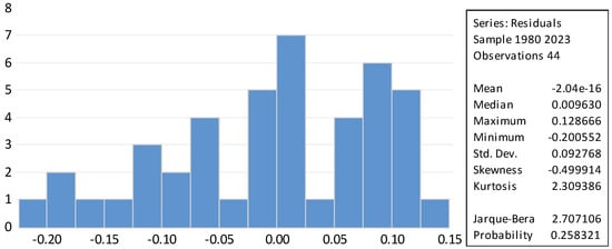
Figure 2.
Normality test. Source: Author’s Computation from Eviews 12 output.
Table 7.
Ramsey Reset test. Source: Authors’ Computation from Eviews 12 output.
From the results presented in the table above, using the Ramsey Reset test, the p-value of 0.491 was greater than the test statistic of 0.05. We fail to reject the null hypothesis at the 5% level of significance and conclude that the model is correctly specified. The Ramsey Reset Test in Table 6 confirms that the model is correctly specified, as both the F-statistic and t-statistic probabilities are greater than 0.05. The model can therefore be said to be fit for interpretation.
4.6. Regression Results
4.6.1. Model 1: Regression Results for the Impact of Exchange Rate Volatility on Imports
Model 1 focuses on the impact of ERV, FDI, and INF on imports (IMP), where IMP is the dependent variable.
The regression results presented in Table 8 above indicate a model analyzing the impact of various independent variables on the dependent variable, imports (IMP). The R-squared 0.780 indicates that approximately 78% of the variance in imports is explained by the independent variables in the model. This is a strong fit, suggesting that the model captures a significant amount of the variability in import levels. The Adjusted R-squared of 0.688 accounts for the number of predictors in the model, indicating that the model remains robust even after adjusting for the number of variables, while the Durbin–Watson statistic 0.786 value suggests potential positive autocorrelation in the residuals, as it is significantly below 2. This could indicate that the model may need further refinement to address potential autocorrelation issues. However, the F-statistic of 9.367 suggests that the model is statistically significant as a whole. The associated p-value (0.000) indicates that at least one of the independent variables is significantly related to the dependent variable.
Table 8.
Regression results for Model 1. Source: Author’s Computation from Eviews 12 output.
4.6.2. Model 2: Regression Results for the Impact of Exchange Rate Volatility on Exports
Model 2 focuses on the impact of ERV, FDI, and INF on exports (EXP), where EXP is the dependent variable.
The regression results for Model 2 in Table 9 above analyze the impact of various independent variables on the dependent variable, exports (EXP). The R-squared of 0.754 indicates that approximately 75.4% of the variance in exports is explained by the independent variables in the model, which is a strong fit. The Adjusted R-squared of 0.666 indicates that even after adjustment, the model remains robust since it is above 50%. The Durbin–Watson statistic: 0.736 value suggests potential positive autocorrelation in the residuals, as it is significantly below 2, indicating that the model may need refinement to address autocorrelation issues. However, the F-statistic 4.890 statistic indicates that the model is statistically significant overall and the p-value (0.002) suggests that at least one of the independent variables is significantly related to exports.
Table 9.
Regression results for Model 2. Source: Authors’ Computation from Eviews 12.
5. Discussion and Conclusions
In a regression model, the constant variable (C), often denoted as βo, the intercept represents the expected value of the dependent variable when all independent variables are equal to zero. From Model 1, the coefficient 1.775 represents the expected value of imports when all independent variables are zero. The t-statistic (29.150) and p-value (0.000) suggest that this coefficient is statistically significant. Meanwhile, in Model 2, the coefficient 1.685 also represents the expected value of exports when all independent variables are zero. The t-statistic (28.556) and p-value (0.000) indicate that this coefficient is statistically significant.
Exchange rate volatility (ERV) was found to be statistically significant in explaining variations in both exports and imports, with significance at the 5% level. The analysis revealed negative coefficients of −5.53 for exports and −2.72 for imports. These findings align with those of Nyunt (2019). who investigated similar dynamics within the ASEAN Member States. Additionally, our results are consistent with earlier studies conducted by Cushman (1983), which examined U.S. trade data, and Peree and Steinherr (1989), who analyzed the effects of ERV in industrialized nations. Chimhore and Chivasa (2021) also concluded a negative relationship when they studied on the impact of exchange rates on exports in Zimbabwe using the ordinary least squares method. In contrast, a study by Mosbei et al. (2021) focused on the impact of exchange rate volatility on intra-East African Community regional trade, revealing a positive relationship as determined through the GARCH model, thereby presenting a divergent perspective from the aforementioned research.
Foreign direct investment (FDI) was determined to be statistically insignificant in explaining changes in both imports (IMP) and exports (EXP), indicating a lack of relationship between foreign direct investment and variations in international trade in Zimbabwe. The result was also found to be consistent with Chimhore and Chivasa (2021). This finding contrasts with the results of Nyunt (2019), who identified a positive relationship between FDI and exports, a conclusion that is also supported by the research conducted by Mosbei et al. (2021).
Inflation (INF) was found to be statistically significant at the 5% level in explaining changes in imports (IMP) and exports (EXP) as dependent variables. The results indicate a negative relationship between inflation variations and changes in both imports and exports in Zimbabwe, with coefficients of −0.005 for imports and −0.042 for exports. In contrast, Nyunt (2019) identified a positive relationship between inflation and exports in his study of ASEAN economies, which contradicts the findings of the present research. Additionally, Mosbei et al. (2021) reported an insignificant relationship between inflation and intra-East African trade, further highlighting the divergence in findings regarding the impact of inflation on trade dynamics. Our evidence refutes Amaglobeli et al. (2022)’s contention that ERV’s trade impacts are dollar-neutral in dollarized economies. Our experience in post-2019 RTGS crisis in Zimbabwe demonstrates that quasi-dollarization itself cannot counteract ERV’s retarding impact on trade if credibility in monetary policy remains low—a gap missing in earlier developing-economy GARCH literature.
5.1. Conclusion and Recommendations
This study aimed to investigate the impact of exchange rate volatility on international trade in Zimbabwe, utilizing time-series data from 1980 to 2023. The primary focus was to determine the significance of exchange rate volatility, foreign direct investment (FDI), and inflation in shaping Zimbabwe’s trade dynamics. The data were sourced from the World Bank and Bruegel.org, with variables expressed as percentages of GDP, and analyzed using OLS methodology in Econometric Views 12. The GARCH model results indicated that some explanatory variables were statistically significant, while others were not. The model passed all diagnostic tests, confirming its robustness, with high R-squared values suggesting that the explanatory variables accounted for a substantial portion of the variance in imports and exports. Overall, this study found that exchange rate volatility negatively affects international trade in Zimbabwe, consistent with the existing literature that highlights the empirical complexities surrounding theoretical predictions in general equilibrium models. To effectively address exchange rate volatility, this study recommends that policies target its root causes rather than merely focusing on fluctuations. Maintaining a flexible exchange rate regime could facilitate more profitable transactions in the foreign exchange market. The government should strive for a stable and competitive exchange rate as part of its trade promotion strategy, implementing policy reforms to enhance international trade competitiveness (Muturi, 2020).
A stable exchange rate fosters certainty for investors and reduces operational risks, while a competitive exchange rate ensures that Zimbabwean goods remain attractive in foreign markets. Ultimately, a combination of stable and competitive currency conditions can attract investment, boost output, and enhance economic prosperity. However, the findings suggest that simply moderating exchange rate volatility may not significantly improve trade performance; effective management of fiscal and monetary shocks is also essential for fostering a stable economic environment conducive to trade growth. Policymakers should develop coherent strategies to establish and maintain a favorable exchange rate system that supports overall trade and economic development.
5.2. Recommendation for Further Studies
There are several important limitations in this study on the ERV–trade nexus for Zimbabwe: using aggregate trade data hides sectoral differences (for example, between mining, which is dollarized and more resilient versus agriculture that is not dollarized and vulnerable); annual data do not capture short-term dynamics; and the GARCH model is useful for analyzing volatility but may miss structural policy shocks (e.g., 2016 bond notes), while quantitative methods do not account for firm-level adaptive strategies. To address these gaps, follow-up studies should (1) disaggregate trade data by sector and size of firms to identify ERV resilience differentials; (2) integrate mixed methods (econometrics plus exporter interviews) to uncover practical barriers to hedging; (3) study the effects of monetary policies in Zimbabwe (such as forex auctions) through comparative studies (for example, with Argentina/Venezuela); and (4) use advanced techniques (threshold GARCH, wavelet analysis) to identify nonlinear ERV effects.
5.3. Research Limitations
The country’s competitiveness from the supply-side perspective is another crucial element, in addition to quantitative factors, in determining export and import performance. This study identified factors such as infrastructure, institutions, macroeconomic stability, labor market policies, skills, and health as important determinants of a nation’s productivity and competitiveness. Schwab (2011) argued that in order to maximize international competitiveness, countries must get these basic elements right. This enables a country to be more competitive by reducing the effort required in the production and distribution processes. However, this study did not provide detailed discussions on the impact of these factors, which could be an area for future research.
Author Contributions
Conceptualization, C.N.C.; Methodology, I.M.; Investigation, I.M.; Writing—original draft, I.M.; Writing—review and editing, C.N.C.; Supervision, C.N.C. All authors have read and agreed to the published version of the manuscript.
Funding
The research did not receive External Funding.
Institutional Review Board Statement
Not applicable.
Informed Consent Statement
Not applicable.
Data Availability Statement
Data are contained within the article.
Conflicts of Interest
The authors declare no conflicts of interest.
References
- Amaglobeli, D., Hanedar, E., Hong, G. H., & Thévenot, C. (2022). Fiscal policy for mitigating the social impact of high energy and food prices (IMF Note No. 2022/001). International Monetary Fund. [Google Scholar] [CrossRef]
- Ameziane, K., & Benyacoub, B. (2022). Exchange rate volatility effect on economic growth under different exchange rate regimes: New evidence from emerging countries using panel CS-ARDL model. Journal of Risk and Financial Management, 15(11), 499. [Google Scholar] [CrossRef]
- Bahmani-Oskooee, M., & Hegerty, S. W. (2007). Exchange rate volatility and trade flows: A review article. Journal of Economic Studies, 34(3), 211–255. [Google Scholar] [CrossRef]
- Bai, J., & Perron, P. (2003). Computation and analysis of multiple structural change models. Journal of Applied Econometrics, 18(1), 1–22. [Google Scholar] [CrossRef]
- Baldwin, R. (2016). The great convergence: Information technology and the new globalization. Harvard University Press. [Google Scholar]
- Berg, A., & Borensztein, E. (2000). The role of foreign direct investment in the economic development of Zimbabwe. World Bank. [Google Scholar]
- Berndt, E. R., Hall, B. H., Hall, R. E., & Hausman, J. A. (1974). Estimation and inference in nonlinear structural models. Annals of Economic and Social Measurement, 3(4), 653–666. [Google Scholar]
- Blanchard, O. (2010). Macroeconomics. Pearson. [Google Scholar]
- Blonigen, B. A. (2005). A review of the empirical literature on FDI determinants. Atlantic Economic Journal, 33(4), 383–403. [Google Scholar] [CrossRef]
- Bollerslev, T. (1986). Generalized autoregressive conditional heteroskedasticity. Journal of Econometrics, 31(3), 307–327. [Google Scholar] [CrossRef]
- Breusch, T. S., & Godfrey, L. G. (1980). A review of recent work on testing for autocorrelation in dynamic economic models. Journal of Econometrics, 13(3), 325–329. [Google Scholar]
- Breusch, T. S., & Pagan, A. R. (1979). A simple test for heteroskedasticity and random coefficient variation. Econometric: Journal of the Econometric Society, 47, 1287–1294. [Google Scholar] [CrossRef]
- Broll, U., & Lockwood, L. (2001). Exchange rate volatility and international trade. International Journal of Finance & Economics, 6(3), 221–233. [Google Scholar]
- Brooks, C. (2019). Introductory econometrics for finance (4th ed.). Cambridge University Press. [Google Scholar]
- Chikwature, W., & Chidhagu, M. (2016). Impact of exchange rate volatility on business performance in Zimbabwe. International Journal of Science and Research, 5(8), 1464–1469. [Google Scholar]
- Chimhore, M., & Chivasa, S. (2021). The effects of exchange rate on Zimbabwe’s Exports. Journal of Economics and Behavioral Studies, 13(4), 8–16. [Google Scholar] [CrossRef]
- Choudhri, E. U., & Hakura, D. (2006). Exchange rate volatility and trade flows: A study of the Zimbabwean economy. Journal of International Trade & Economic Development, 15(3), 345–367. [Google Scholar]
- Chow, G. C. (1960). Tests of equality between sets of coefficients in two linear regressions. Econometrica, 28(3), 591–605. [Google Scholar] [CrossRef]
- Cushman, D. O. (1983). The effects of real exchange rate risk on international trade. Journal of International Economics, 15(1–2), 45–63. [Google Scholar] [CrossRef]
- Dimitrios, N., Antonios, A., Konstantinos, S., & Ioannis, G. (2016). The impact of exchange rate volatility on exports: Evidence from selected EU member countries. Palgrave Macmillan. [Google Scholar]
- Dornbusch, R. (1980). Exchange rate economics: Where do we stand? Brookings Papers on Economic Activity, 1980(1), 143–185. [Google Scholar] [CrossRef]
- Dornbusch, R. (1988). Real exchange rates and macroeconomics: A selective survey. The Scandinavian Journal of Economics, 90(2), 401–432. [Google Scholar]
- Engle, R. F. (1982). Autoregressive conditional heteroscedasticity with estimates of the variance of United Kingdom inflation. Econometrica, 50(4), 987–1007. [Google Scholar] [CrossRef]
- Ethier, W. J. (1973). International trade and the forward exchange market. The American Economic Review, 63(3), 494–503. [Google Scholar]
- Frenkel, J. A. (1976). A monetary approach to the exchange rate: Doctrinal aspects and empirical evidence. The Scandinavian Journal of Economics, 78(2), 200–224. [Google Scholar] [CrossRef]
- Froot, K. A., & Stein, J. C. (1991). Exchange rates and foreign direct investment: An imperfect capital markets approach. The Quarterly Journal of Economics, 106(4), 1191–1217. [Google Scholar] [CrossRef]
- Gopinath, G. (2020). The future of trade: A new trade policy for a new world. Journal of International Economics, 125, 1–11. [Google Scholar]
- Gujarati, D. N., & Porter, D. C. (2009). Basic econometrics (5th ed.). McGraw-Hill. [Google Scholar]
- Hanke, S. H., & Kwok, A. K. F. (2009). On the measurement of Zimbabwe’s hyperinflation. Cato Journal, 29(2), 353–364. [Google Scholar]
- Ilzetzki, E., Reinhart, C. M., & Rogoff, K. S. (2023). Exchange rate dynamics and the impact on global trade. The Quarterly Journal of Economics, 138(2), 455–512. [Google Scholar]
- International Monetary Fund (IMF). (2016). Annual report. Available online: https://www.imf.org/external/pubs/ft/ar/2016/eng/pdf/ar16_eng.pdf (accessed on 22 June 2025).
- Joseph, D. N., Oswald, A., & Charles, A. A. (2014). The impact of exchange rate movement on export: Empirical evidence from Ghana. International Journal of Academic Research in Accounting, Finance and Management Sciences, 4(3), 41–48. [Google Scholar]
- Kanyenze, G., Chitambara, P., & Mupedziswa, R. (2017). The Zimbabwe economy: A review of the economic performance and policy framework. Zimbabwe Economic Policy Analysis and Research Unit. [Google Scholar]
- Khosa, J., Botha, I., & Pretorius, M. (2015). The impact of exchange rate volatility on emerging market exports. Acta Commercii, 15(1), 257. [Google Scholar] [CrossRef]
- Krugman, P. R., & Obstfeld, M. (2009). International economics: Theory and policy. Pearson. [Google Scholar]
- Markusen, J. R. (2002). Multinational firms and the theory of international trade. MIT Press. [Google Scholar]
- McKenzie, M. D. (1999). The impact of exchange rate volatility on international trade: A review of the literature. Journal of Economic Surveys, 13(1), 1–29. [Google Scholar] [CrossRef]
- Mhaka, S. (2019). The impact of exchange rate volatility on Zimbabwean firms’ competitiveness. African Journal of Business and Economic Research, 14(1), 167–184. [Google Scholar]
- Michael, P., Nobay, R. A., & Peel, D. A. (2004). Purchasing power parity yet again: Evidence from a new test. Journal of International Money and Finance, 23(4), 627–650. [Google Scholar]
- Mlambo, C., & Moyo, T. (2020). The impact of exchange rate fluctuations on trade in Zimbabwe. African Journal of Economic and Management Studies, 11(2), 171–183. [Google Scholar]
- Mosbei, T., Samoei, K. S., Tison, C. C., & Kipchoge, E. K. (2021). Exchange rate volatility and its effect on intra-East Africa Community regional trade. Latin American Journal of Trade Policy, 4(9), 43–53. [Google Scholar] [CrossRef]
- Mpofu, R. T. (2019). The impact of exchange rate volatility on the competitiveness of Zimbabwean firms. African Journal of Management, 5(2), 154–167. [Google Scholar]
- Muturi, W. (2020). Determinants of exchange rate volatility in Kenya. International Journal of Social Science and Humanities Research (IJSSHR), 2(2), 235–244. [Google Scholar] [CrossRef]
- Nyunt, L. K. (2019). The impact of exchange rate volatility on international trade: Evidence from ASEAN member states. Available online: https://archives.kdischool.ac.kr/handle/11125/34182 (accessed on 22 June 2025).
- Onafowora, O., & Owoye, O. (2008). Exchange rate volatility and export growth in Nigeria. Applied Econometrics and International Development, 8(1), 167–180. [Google Scholar] [CrossRef]
- Peree, E., & Steinherr, A. (1989). Exchange Rate Stability and Trade Flows. Journal of International Money and Finance, 8(4), 425–440. [Google Scholar]
- Perron, P. (2006). Dealing with structural breaks. In T. C. Mills, & K. Patterson (Eds.), Palgrave handbook of econometrics (Vol. 1, pp. 278–352). Palgrave Macmillan. [Google Scholar]
- Rodrik, D. (2021). The globalization paradox: Democracy and the future of the world economy. W. W. Norton & Company. [Google Scholar]
- Schwab, K. (2011). The global competitiveness report 2011–2012. World Economic Forum. [Google Scholar]
- World Bank. (2023). Zimbabwe economic update: Navigating economic challenges. World Bank Publications. [Google Scholar]
- Zimbabwe National Statistics Agency (ZIMSTAT). (2018). Annual trade report. Zimbabwe National Statistics Agency. [Google Scholar]
Disclaimer/Publisher’s Note: The statements, opinions and data contained in all publications are solely those of the individual author(s) and contributor(s) and not of MDPI and/or the editor(s). MDPI and/or the editor(s) disclaim responsibility for any injury to people or property resulting from any ideas, methods, instructions or products referred to in the content. |
© 2025 by the authors. Licensee MDPI, Basel, Switzerland. This article is an open access article distributed under the terms and conditions of the Creative Commons Attribution (CC BY) license (https://creativecommons.org/licenses/by/4.0/).