Inflation Forecasting: LSTM Networks vs. Traditional Models for Accurate Predictions

Abstract

This study investigates the effectiveness of neural network models, particularly LSTM networks, in enhancing the accuracy of inflation forecasting. We compare LSTM models with traditional univariate time series models such as SARIMA and AR(p) models, as well as machine learning approaches like LASSO regression. To improve the standard LSTM model, we apply advanced feature selection techniques and introduce data augmentation using the MBB method. Our analysis reveals that LASSO-LSTM hybrid models generally outperform LSTM models utilizing PCA for feature selection, particularly in datasets with multiple features, as measured by RMSE. However, despite these enhancements, LSTM models tend to underperform compared to simpler models like LASSO regression, AR(p), and SARIMA in the context of inflation forecasting. These findings suggest that, for policymakers and central bankers seeking reliable inflation forecasts, traditional models such as LASSO regression, AR(p), and SARIMA may offer more practical and accurate solutions.

1. Introduction

Inflation forecasting has been central to macroeconomic research, with traditional models like the Phillips curve offering insights into the relationship between inflation and unemployment. However, these models have shown limitations in capturing the complexities of modern economies. Recent studies suggest that incorporating financial variables, commodity prices, and broader economic indicators can enhance forecasting accuracy (Atkeson et al., 2001; Chen et al., 2014; Forni et al., 2003; Groen et al., 2013; Staiger et al., 1997). As central banks increasingly rely on multivariate models to inform monetary policy, the demand for more sophisticated approaches has grown. One well-established approach in inflation forecasting is the use of multivariate time series models such as (Stock & Watson, 2008). These models integrate a wide range of economic indicators to predict inflation more accurately. However, despite the inclusion of additional variables, these models often struggle to outperform simpler univariate models like SARIMA out-of-sample. In response to these challenges, machine learning techniques have been applied to inflation forecasting, though with mixed results. Long Short-Term Memory (LSTM) models, for instance, have demonstrated some potential in capturing non-linearities and long-term trends but have not consistently outperformed traditional models like SARIMA (Paranhos, 2024).

Recent research highlights the importance of model selection and the inclusion of relevant data in improving forecasting performance. Machine learning methods such as Quantile Random Forests (Lenza et al., 2023) and LSTM-based models have shown that while these approaches can be powerful, they are also prone to overfitting and lack interpretability, making them less useful for policy applications. This has led to renewed interest in hybrid approaches that combine machine learning with more interpretable models like LASSO to enhance both accuracy and transparency. In this study, we aim to address the limitations of existing machine learning models in inflation forecasting by employing a hybrid model that combines LSTM’s ability to capture long-term dependencies with LASSO’s feature selection capabilities. LASSO reduces dimensionality by focusing on relevant variables, enhancing interpretability, and mitigating overfitting. By incorporating financial variables and commodity prices alongside traditional economic indicators, we aim to improve forecast accuracy over both short- and long-term horizons. We compare the performance of our LASSO-LSTM model to benchmarks such as univariate models, as well as machine learning techniques.

This study offers several novel contributions to the growing literature on inflation forecasting with machine learning. First, we introduce a LASSO-LSTM hybrid model that leverages the strengths of both techniques—LASSO for robust feature selection and LSTM for capturing temporal dependencies. While previous studies, such as (Paranhos, 2024) and (Almosova & Andresen, 2023), examine LSTM models in macroeconomic contexts, they do not combine them with regularization-based feature selection or explicitly contrast them against multiple machine learning and traditional benchmarks within a sequential updating framework. Our findings indicate that, despite the sophisticated capabilities of machine learning models, simpler models like LASSO regression, AR(p), and SARIMA often outperform LSTM networks in forecasting inflation. This is consistent with previous research, suggesting that LSTM models may underperform compared to univariate models and other machine learning methods in certain contexts. These results suggest that for policymakers and central bankers seeking reliable and interpretable inflation forecasts, traditional models such as LASSO regression, AR(p), and SARIMA may be more suitable choices. The relative simplicity and transparency of these models can provide clearer insights into inflation dynamics, facilitating more informed decision-making.

Second, our study systematically compares LSTM variants (standard, LASSO-selected, PCA-selected, and data-augmented via MBB) with classical models such as SARIMA and AR(p), as well as other ML models like Ridge and Random Forest, across short-, medium-, and long-term forecast horizons. This structured benchmarking, combined with a robust evaluation across multiple time periods, offers a comprehensive and dynamic out-of-sample assessment not found in earlier work.

Third, by incorporating financial data from both FRED-MD and EIKON and exploring data augmentation techniques tailored for macroeconomic time series, we address a key limitation in the LSTM literature: small sample size. Our findings provide nuanced insights into when and why LSTM models fail to outperform simpler models, highlighting overfitting, gradient instability, and lack of transparency as key factors, thereby contributing not only empirical results but also theoretical clarity.

The rest of this paper is organized as follows: Section 2 reviews relevant literature, Section 3 presents the data, Section 4 discusses the models, Section 5 presents and discusses results, and Section 6 concludes our work.

2. Literature Review

2.1. Inflation Forecasting with Classical Methods

Inflation-targeting regimes were adopted by many countries in the late 1980s and early 1990s, prompting central banks to place increased emphasis on inflation forecasts in the formulation of monetary policy. To support these efforts, a variety of forecasting models have been employed, including Vector Autoregressive (VAR) models, Dynamic Stochastic General Equilibrium (DSGE) models, and factor models. However, the performance of these models has varied across economic conditions. During the global financial crisis and the subsequent recovery period, Iversen et al. (2016) observed that DSGE models exhibited significant forecast biases, particularly in projecting inflation and interest rates. In contrast, Bayesian VAR (BVAR) models produced more reliable forecasts, with notably lower biases in these key macroeconomic indicators (Iversen et al., 2016).

The Phillips curve, which connects inflation and unemployment, has been a foundational model for inflation forecasting. However, Atkeson et al. (2001) demonstrated that Phillips curve models often fail to outperform simpler naive models that predict future inflation based on past trends. This criticism has spurred research into alternative approaches, with findings suggesting that Phillips curve models struggle to capture the non-linear dynamics of inflation, especially during periods of significant economic change (Fisher et al., 2002).

Despite their simplicity, ARIMA models have demonstrated strong performance in short-term forecasting tasks. Meyler et al. (1998) emphasize that while ARIMA models minimize out-of-sample forecast errors, they lack theoretical grounding and are backward-looking, limiting their ability to predict turning points. Similarly, Robinson (1998) noted that VAR models are effective at capturing relationships between multiple economic variables and are widely used by central banks. However, these models can struggle in periods of structural change or economic volatility.

2.2. Inflation Forecasting with Machine Learning

The limitations of traditional models have motivated the exploration of machine learning methods for inflation forecasting. Deep learning models, particularly LSTM networks, have gained attention due to their ability to capture long-term dependencies in data. Theoharidis et al. (2023) argue that LSTM models can outperform traditional methods, particularly at longer horizons, but they also note that deep learning models are prone to overfitting and lack transparency.

Almosova and Andresen (2023) employ LSTM models to forecast U.S. inflation and find that their performance is comparable to that of SARIMA and other machine learning models, particularly at longer forecast horizons. They highlight that LSTM models are sensitive to training sample size and hyperparameter choices, and tend to underperform due to their tendency to overfit when applied to economic time series with relatively low frequency and high persistence.

Several studies further benchmark LSTM for forecasting in different domains. Yadav et al. (2020) apply LSTM models to financial time series and demonstrate that careful hyperparameter tuning can enhance predictive performance. However, they also emphasize the lack of established guidelines for configuring such models effectively. The authors in (Song et al., 2020) use LSTM models with a limited set of features to forecast oil well production and report high predictive accuracy. Similarly, Siami-Naimi et al. (2019) find that bidirectional LSTM (BiLSTM) models can outperform both standard LSTM and ARIMA models across various forecasting tasks, underscoring the value of directional memory in sequential learning.

Inflation studies using machine learning methods are also emerging. Sengüler and Kara (2025) examine artificial neural networks for inflation forecasting in Turkey and find that ML-based approaches provide significant advantages over linear models. Araujo and Gaglianone (2023) benchmark various machine learning techniques as well as traditional methods for inflation forecasting in Brazil, concluding that while neural networks and ensemble methods offer improvements over traditional models, the performance varies widely depending on input selection and forecast horizon.

Despite their potential, LSTM models have not consistently outperformed simpler approaches such as SARIMA or Random Forest in the context of inflation forecasting. (Paranhos, 2024) conducts a systematic evaluation of deep learning models for inflation forecasting in the euro area, emphasizing the limitations of LSTM architectures when applied to macroeconomic data. Despite experimenting with a range of input variables and network configurations, the study finds that LSTM models fail to outperform traditional benchmarks such as SARIMA and Bayesian VAR, particularly at short forecast horizons. This suggests that although LSTM models are effective at capturing long-term trends, they may not always be the optimal choice for short-term inflation forecasting, particularly when compared to simpler linear models.

The integration of feature selection techniques with machine learning has emerged as a promising approach. Garcia et al. (2017) demonstrated that LASSO, a shrinkage method, performs especially well in data-rich environments by mitigating overfitting and enhancing forecast accuracy for short-term inflation. By focusing on the most relevant predictors, LASSO-based models can simplify complex datasets and enhance the interpretability of machine learning models.

2.3. The Role of Financial and Commodity Variables in Inflation Forecasting

Stock and Watson (2003) emphasized that asset prices—such as interest rates and stock returns—can serve as valuable indicators of future inflation, although their predictive power varies across different periods and countries. Financial variables, including spreads and exchange rates, have also been identified as significant contributors to the accuracy of inflation forecasts (Forni et al., 2003).

Commodity prices, particularly in small commodity-exporting countries, have demonstrated strong predictive power for inflation. Chen et al. (2014) found that aggregates of world commodity prices outperformed alternative models, especially in forecasting Consumer Price Index (CPI) and Producer Price Index (PPI) inflation in these economies. Incorporating such variables has been shown to enhance the robustness of inflation forecasts, notably in economies with high reliance on commodity exports.

2.4. Motivation for Hybrid Models

Given the limitations of both classical and machine learning models, hybrid approaches that leverage the strengths of each have gained increasing attention. In particular, hybrid models that combine feature selection methods like LASSO with deep learning architectures such as LSTM offer a compelling balance between accuracy and interpretability. By selecting relevant variables, these models help reduce overfitting and enhance predictive performance, especially in volatile economic environments. Building on this emerging trend, our study tests a LASSO-LSTM model that incorporates financial variables and employs data augmentation techniques—specifically Moving Block Bootstrapping (MBB)—to improve out-of-sample forecasting accuracy and robustness.

3. Data

We collected data from the FRED-MD and the EIKON databases. We obtained macroeconomic and financial data from FRED-MD and financial data from EIKON, which provides us with a broad coverage of inflation indicators.

3.1. Variable-Selection

Feature selection is a critical step in predictive modeling, especially when dealing with datasets where the number of variables exceeds the number of observations—a challenge commonly known as the high-dimensionality problem. Without effective feature selection, models are prone to overfitting, which can degrade their ability to generalize and introduce unnecessary noise into the results.

LASSO addresses this issue by combining variable selection with regularization, effectively reducing model complexity while retaining the most influential predictors. As illustrated in Figure 1, LASSO shrinks the coefficients of less important variables to zero, thereby excluding them from the model. This not only enhances predictive accuracy but also improves interpretability by simplifying the model structure.

3.2. FRED-MD Database

The FRED-MD dataset, compiled by McCracken and Ng, contains monthly U.S. macroeconomic data. For our analysis, we use the version updated in December 2023, which includes 128 variables with 768 observations spanning from January 1959 to December 2023. Before estimating our models, the data undergo a series of preprocessing steps to ensure stationarity, a necessary condition for reliable forecasting. Non-stationary variables are differenced to achieve stationarity, with annual changes computed as $X_t-X_{t-12}$. For key variables such as the Consumer Price Index (CPI), we conduct Augmented Dickey-Fuller (ADF) tests to formally assess stationarity. We also address missing data using the Last Observation Carried Forward (LOCF) method, whereby missing values are replaced with the most recent available observation. This approach is widely used in macroeconomic time series with relatively low rates of missingness. While LOCF offers simplicity and maintains historical continuity, we acknowledge that it may introduce bias, especially when missingness is non-random or occurs during periods of heightened volatility.

3.3. EIKON Database

EIKON is a well-regarded database that is used extensively in academia. It includes global economic, company, and financial data. Data retrieved from this database includes some US commodities like gold, platinum, oil, gas, and corn, as well as shipping rates and Baker Hughes. We retrieved monthly data for the period January 1960 until December 2023 from the Refinitiv EIKON database. In total we included and combined 27 financial variables from EIKON and FRED-MD to create a new dataset with financial data. Some descriptive statistics are presented in Figure 2 below. Using a wide range of financial variables allows us to capture these diverse sources of inflationary pressure. No single variable can reflect the full complexity of global inflation dynamics. Data alignment of EIKON data with FRED-MD is no issue, as the data frequency used is the same. Further details on the data are included in the Appendix A.

Forni et al. (2003) emphasize the importance of financial variables and commodity prices in inflation forecasting, and support our belief that including these time series can improve the accuracy of inflation forecasts. Machine learning models have demonstrated enhanced performance when trained on diverse, high-dimensional datasets, as the richness and variety of features enable these models to capture complex patterns and improve predictive accuracy.

4. Models

4.1. LASSO

Inflation forecasting typically employs huge datasets containing a lot of variables, some of which may be irrelevant for prediction purposes. The Least Absolute Shrinkage and Selection Operator (LASSO) has the ability to select only the most important covariates, discarding irrelevant information and keeping the error of the prediction as small as possible (Freijeiro-González et al., 2022).

LASSO combines properties from both subset selection and ridge regression. This makes it able to produce explicable models (like subset selection), and be as stable as a ridge regression. LASSO minimizes the residual sum of squares while constraining the sum of the absolute values of the coefficients to be less than a specified constant. This constraint causes LASSO to shrink some coefficients exactly to zero, effectively performing variable selection and resulting in more interpretable models (Tibshirani, 1996).

The Lasso model contains:

Data

$$(x^i,y_i),i=1,2,\dots ,N$$

predictor variables

$$x^i={(x_{il},\dots ,x_{ip})}^T$$

and responses

$$y_i$$

We either assume that the observations are independent or that the $y_i$s are conditionally independent given the $x_{ij}$s.

We assume that the $x_{ij}$s are standardized so that

$$\left({\displaystyle \frac{{\sum }_i{x}_{ij}}{N}}\right)=0,{\displaystyle \frac{{\sum }_i{x}_{ij}^2}{N}}=1$$

Letting $\widehat{B}={(\widehat{B_1},\dots ,\widehat{B_p})}^T,$ the lasso estimate $(\widehat{\alpha },\widehat{B})$ is obtained by solving the following optimization problem:

$$(\widehat{\alpha },\widehat{B})=argmin[\sum _{i=1}^N{(y_i-\alpha -\sum _j{\beta }_j{x}_{ij})}^2]$$

subject to

$$\sum _j|{\beta }_j|⩽t$$

Here, $t\ge 0$ is a tuning parameter. Now, for all t, the solution for $\alpha$ is $\widehat{\alpha }=\overline{y}$. We can assume without loss of generality that $\overline{y}=0$ and hence omit $\alpha$.

The parameter $t\ge 0$ controls the amount of shrinkage that is applied to the estimates. Let $\widehat{B_j^0}$ be the full least squares estimates and let $t_0=\sum |\widehat{B_j^0}|$. Values of $t<t_0$ will cause shrinkage of the solutions toward 0, and some coefficients may be exactly equal to 0. For example, if $t=t_0/2$, the effect will be roughly similar to finding the best subset of size $p/2$. It is not necessary for the design matrix to be of full rank for the model to be specified (Tibshirani, 1996).

We include LASSO in our model to address overfitting and optimism bias. LASSO regression aims to identify the subset of variables and their associated coefficients that minimize prediction error by imposing a penalty on the regression coefficients. This penalty shrinks coefficients toward zero by constraining the sum of their absolute values to be less than a fixed threshold, controlled by the regularization parameter ($\lambda$). As a result, less important variables receive coefficients exactly equal to zero, effectively performing variable selection and enhancing model generalizability.

$$(\widehat{\alpha },\widehat{B})=argmin[\sum _{i=1}^N{(y_i-\alpha -\sum _j{\beta }_j{x}_{ij})}^2+\lambda \sum _j|{\beta }_j|]$$

After the shrinkage, variables with regression coefficients equal to zero are excluded from the model (Ranstam & Cook, 2018).

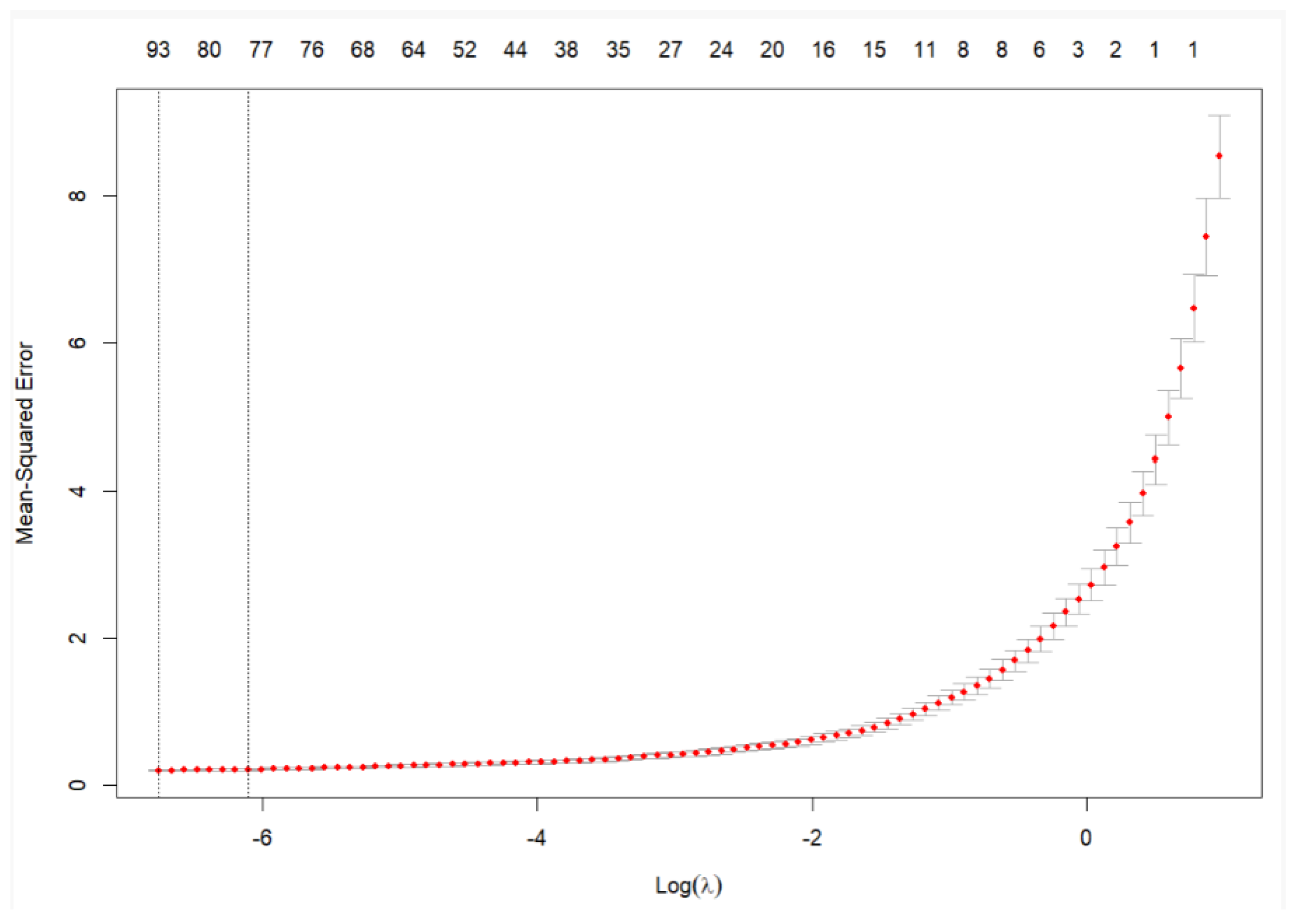
We employ an automated k-fold cross-validation procedure to select the optimal value of $\lambda$. In this approach, the dataset is randomly partitioned into k equally sized subsets. For each iteration, $k-1$ subsets are used to train the model, while the remaining subset is used for validation. This process is repeated k times, with each subset serving once as the validation set. The cross-validation error is computed for a range of $\lambda$ values, and the value of $\lambda$ that minimizes the average validation error across the k folds is selected. This chosen $\lambda$ is then used to estimate the final model.

This technique reduces overfitting without the need to reserve a subset of the dataset exclusively for internal validation. A disadvantage of the LASSO approach is that one may not be able to reliably interpret the regression coefficients in terms of independent risk factors since the focus is on the best combined prediction and not on the accuracy of the estimation (Ranstam & Cook, 2018).

4.2. LSTM

As depicted in Figure 3, the LSTM model is a variant of recurrent neural networks (RNNs) (Almosova & Andresen, 2023). Unlike other neural networks, a recurrent neural network updates by time step. This means that the model will adjust forecasts based on previous time steps. RNN models have proven particularly useful for data-sensitive sequences such as time series analysis, natural language processing, and sound recognition (Mullainathan & Spiess, 2017). For example, in the context of music recognition, one could observe a pattern in the sound, making it possible to predict what is to come next or which song you are listening to (Bishop, 2006). For such models it is crucial that there is a pattern in the data, and that the sequence of the data anticipates later values.

The RNN model is able to update its memory based on previous steps and consider long-term trends and patterns in the data (Tsui et al., 2018). Consider an abnormal drop in inflation for one month, which deviates from previous time steps in the data. The RNN takes into account the underlying pattern in the data based on previous observations, and considers the fall in inflation as an abnormality. What makes inflation behavior abnormal, and which patterns the model detects to label the drop in inflation as abnormal, is inherently difficult to grasp.

LSTM, on the other hand, differs from other RNNs as it possesses an enhanced capability of capturing long-term trends in the data (Tsui et al., 2018). Consider an inflationary episode from the 1970s that exhibits a similar pattern to a recent event. An LSTM model is capable of recognizing these historical similarities in temporal patterns and incorporating them into its forecasting process. However, it does not assign equal weight to all past events. Instead, the influence of the historical episode is modulated based on its relevance, with more emphasis typically placed on recent observations. This dynamic weighting allows LSTM to integrate both long-term dependencies and short-term fluctuations, enabling it to capture complex temporal relationships and generate more contextually informed predictions (Lenza et al., 2023).

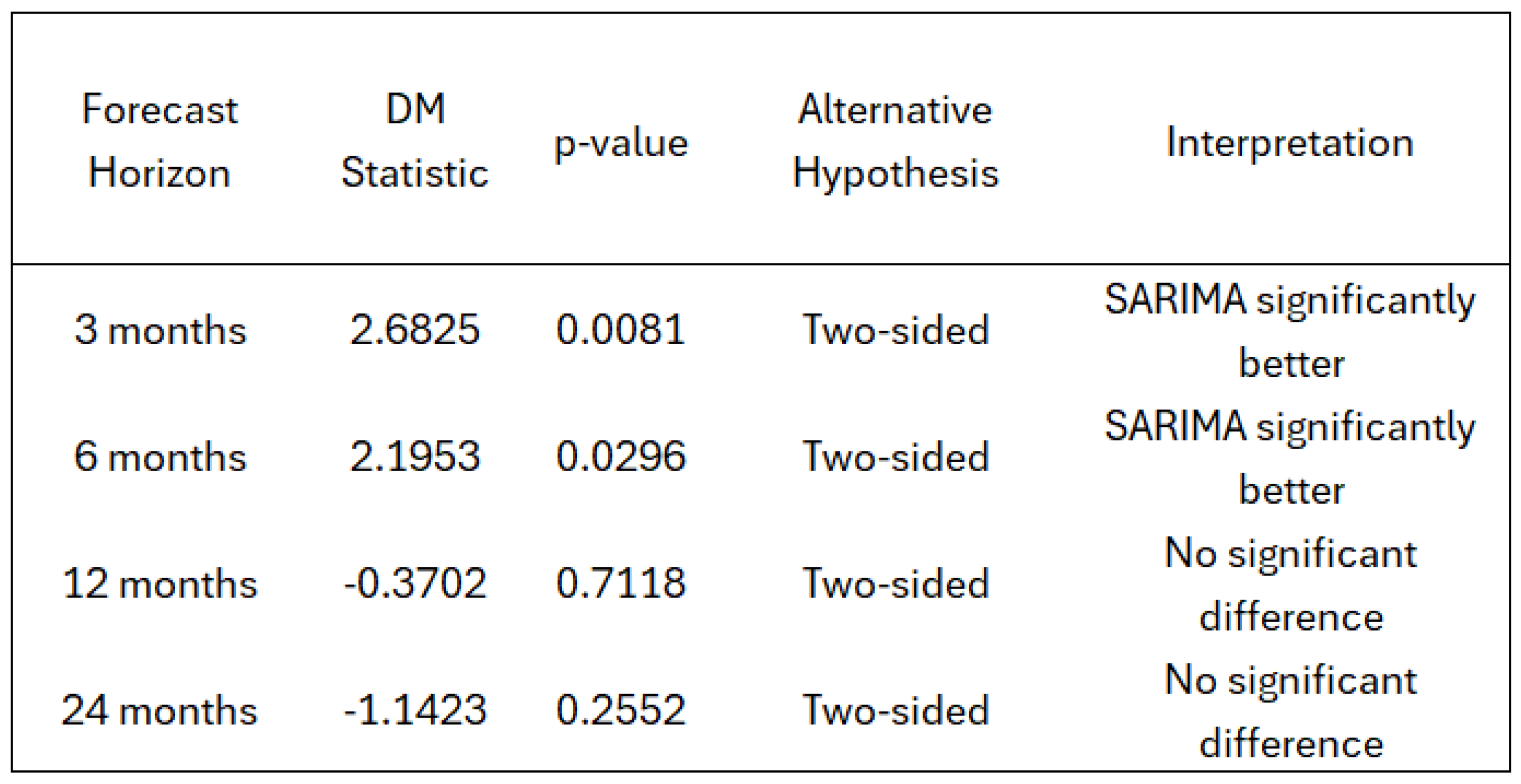
LSTM has proven to be highly efficient for sequential data and has been used to compute univariate forecasts of monthly US CPI inflation. LSTM slightly outperforms autoregressive models (AR), Neural Networks (NN), and Markov-switching models, but its performance is on par with the SARIMA model (Almosova & Andresen, 2023). Recently, it has become harder to outperform naive univariate random walk-type forecasts of US inflation, but since the mid-80s, inflation has also become less volatile and easier to predict. Atkeson et al. (2001) show that averaging over the last 12 months gives a more accurate forecast of the 12-month-ahead inflation than a backward-looking Phillips curve. Macroeconomic literature argues that the inflation process might be changing over time, making a non-linear model more precise in predicting inflation. Basically, there are four main advantages of the LSTM method (Almosova & Andresen, 2023).

1. LSTMs are flexible and data-driven. It means that researchers do not have to specify the exact form of the non-linearity. Instead, the LSTM will infer this from the data itself.

2. Under some mild regulatory conditions, LSTMs and neural networks of any type, in general, can approximate any continuous function arbitrarily accurately. At the same time, these models are more parsimonious than many other non-linear time series models.

3. LSTMs were developed specifically for sequential data analysis and have proved to be very successful with this task.

4. The recent development of the optimization routines for NNs and the libraries that employ computer GPUs has made the training of NNs and recurrent neural networks significantly more feasible.

In contrast to classical time series models, the LSTM network does not suffer from data instabilities or unit root problems. Nor does it suffer from the vanishing gradient problem of general RNNs, which can destroy the long-term memory of these networks. LSTM may be applied to forecasting any macroeconomic time series, provided that there are enough observations to estimate the model.

LSTMs perform particularly well at long horizons and during periods of high macroeconomic uncertainty. This is due to their lower sensitivity to temporary and sudden price changes compared to traditional models in the literature. One should note that their performance is not outstanding, for instance, compared to the random forest model (Lenza et al., 2023). A simplified, visual representation of an LSTM recurrent structure is provided in Figure 4.

A common weakness of machine learning techniques, including neural networks, is the lack of interpretability (Mullainathan & Spiess, 2017). For inflation in particular this could be a problem, since much of the effort is devoted to understanding the underlying inflation process, sometimes at the expense of marginal increases in forecasting gains. LSTM is, on average, less affected by sudden, short-lived movements in prices compared to other models. Random forest has proved sensitive to the downward pressure on prices caused by the global financial crisis (GFC). Machine learning models are more prone to instabilities in performance due to their sensitivity to model specification (Almosova & Andresen, 2023). This also applies to the LSTM network. Lastly, LSTM-implied factors display high correlation with business cycle indicators, informing on the usefulness of such signals as inflation predictors.

The LSTM model is characterized by two key components: the cell state, which acts as the long-term memory, and the hidden state, representing the short-term memory. A schematic representation of an LSTM cell is provided in Figure 5. Initially, both states are assigned default values (often zeros), and they are subsequently updated as new input sequences are processed. The model uses sigmoid and tanh activation functions within its gating mechanisms—namely the input, forget, and output gates—to regulate the flow of information. These functions determine how much of the new input is retained, how much of the previous state is forgotten, and how the internal memory is updated, thereby enabling the LSTM to capture complex temporal dependencies over time.

4.3. LASSO-LSTM

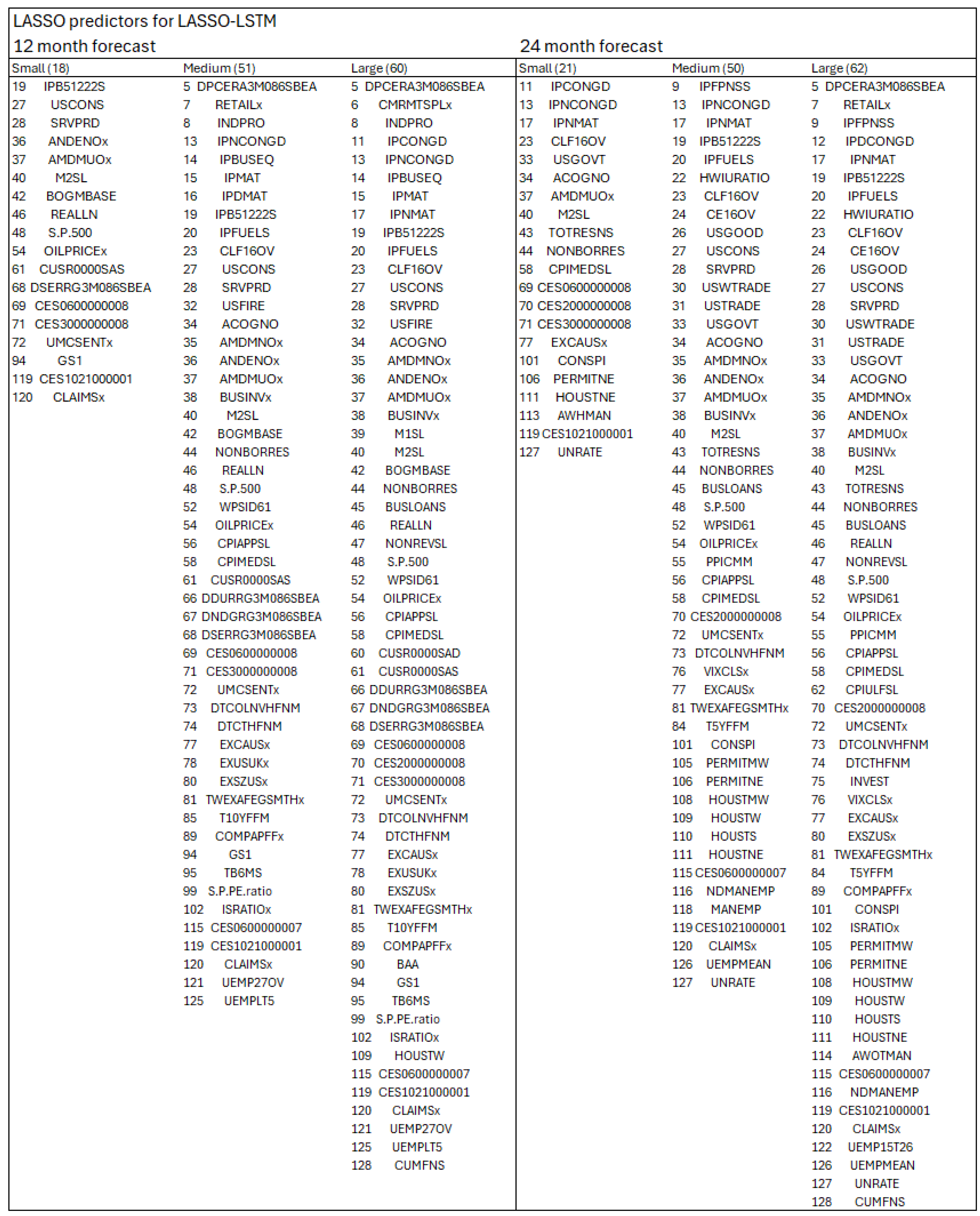
The LASSO-LSTM model is a hybrid machine learning framework that combines the strengths of LASSO regression and Long Short-Term Memory (LSTM) networks. The process begins with LASSO, which serves as a feature selection mechanism. Unlike ordinary least squares (OLS), LASSO introduces a penalty $\lambda$ on the regression coefficients, shrinking less informative coefficients toward zero and effectively excluding irrelevant predictors from the model. This dimensionality reduction mitigates overfitting and enhances interpretability. The selected subset of predictors is then used to train the LSTM, which captures temporal dependencies and non-linear patterns in the data. The regularization parameter $\lambda$ in LASSO plays a critical role, as it directly influences the number and type of features passed to the LSTM, thereby shaping the final model’s complexity and performance.

In this study, the regularization parameter $\lambda$ is calibrated at three distinct levels—small, medium, and large—corresponding to LASSO-LSTM architectures of varying complexity. A larger regularization term leads to greater coefficient shrinkage in the LASSO step, resulting in fewer selected predictors and thus a smaller and more constrained LSTM architecture. This multi-scale approach allows us to systematically evaluate the trade-off between underfitting and overfitting in the context of macroeconomic forecasting. By comparing model performance across architectures, we gain insight into how regularization impacts predictive accuracy and model generalization under different data conditions.

LSTM models, while effective at capturing complex temporal patterns, are prone to overfitting in medium-sized, high-dimensional macroeconomic datasets. As shown by (Paranhos, 2024), larger LSTM architectures do not always outperform smaller ones. To mitigate this, LASSO is applied for feature selection, retaining only the most relevant predictors and improving model efficiency and generalization.

The selected features feed into the LSTM input layer. Architecture size is adjusted based on regularization strength: larger models, more susceptible to overfitting, are constrained with fewer layers and dropout applied; smaller models, less prone to overfitting, allow for more layers and reduced dropout. The LASSO-LSTM thus combines feature selection and temporal modeling to enhance predictive performance while controlling complexity.

An alternative and widely used method for feature reduction is Principal Component Analysis (PCA) (Tsui et al., 2018). While both PCA and LASSO aim to manage high-dimensional data, their objectives and implications differ. PCA identifies components that explain the greatest variance in the data, often resulting in linear combinations of variables that lack direct interpretability. In contrast, LASSO performs variable selection by shrinking less relevant coefficients toward zero, retaining only the most influential predictors. This feature selection preserves interpretability, making LASSO-LSTM particularly valuable in policy contexts, where understanding which variables drive the forecast is essential, especially for central banks and decision-makers.

4.4. ARIMA and SARIMA

Seasonal Autoregressive Integrated Moving Average (SARIMA) extends the ARIMA model by explicitly accounting for seasonality in time series data. While ARIMA assumes either non-seasonal data or that seasonal patterns have been removed—typically through seasonal differencing—SARIMA incorporates seasonal terms directly, enabling more accurate modeling of data with recurring cycles (Dubey et al., 2021).

An ARIMA(p, d, q) model can be represented by Equation (1) below:

$$\begin{array}{cc}\hfill {\Delta }^d{Y}_t& ={\beta }_0+\sum _{i=1}^p{\varphi }_i{Y}_{t-i}+\sum _{j=1}^q{\theta }_j{e}_{t-j}+e_t\hfill \end{array}$$

(1)

Here ${\beta }_0$ is a constant, ${\varphi }_i$ are the coefficients of the autoregressive part with p lags, ${\theta }_j$ are the coefficients of the moving average part with q lags, and $e_t$ is the error term at time t. The error terms are typically assumed to be i.i.d. variables drawn from a normal distribution with zero mean.

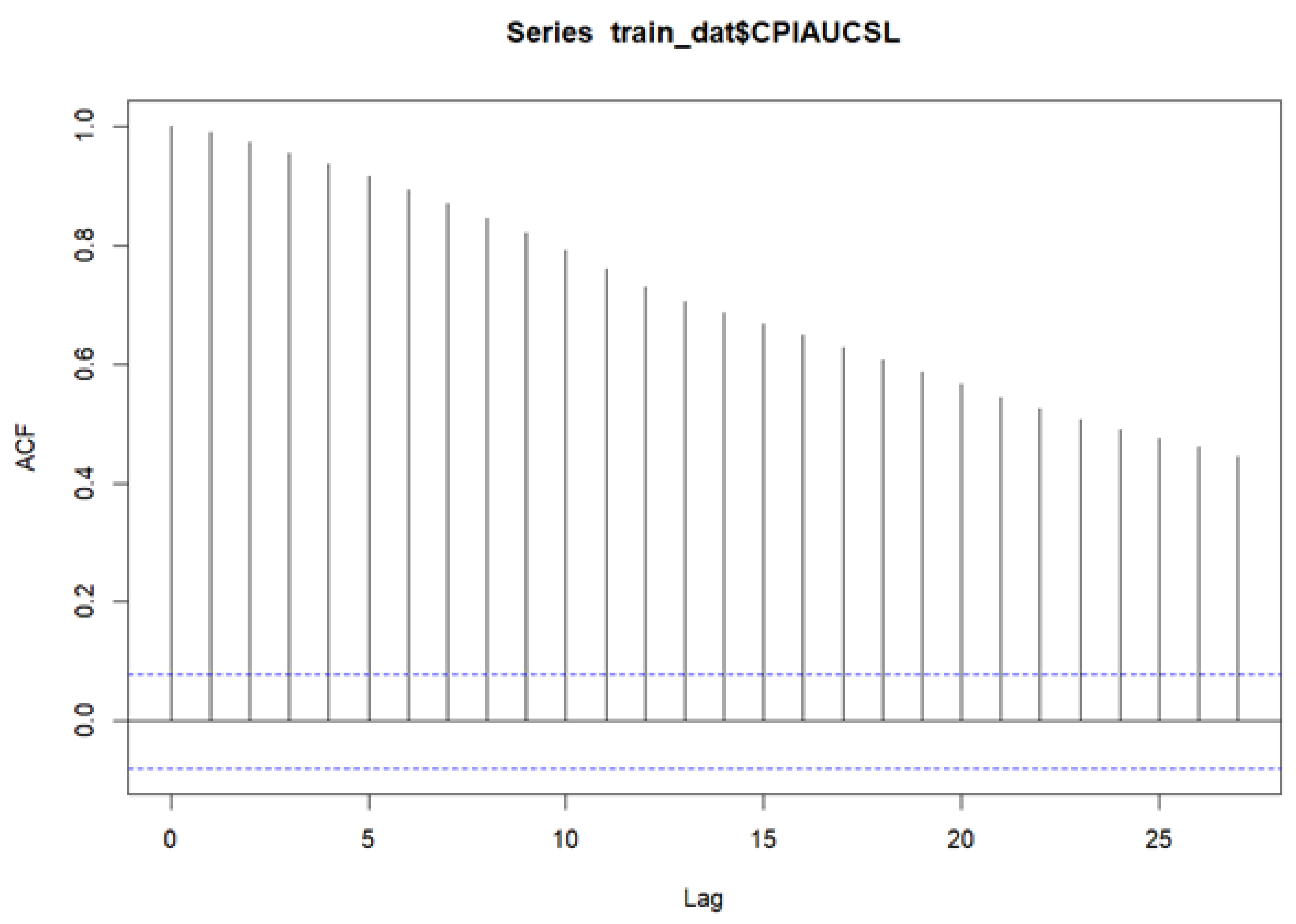
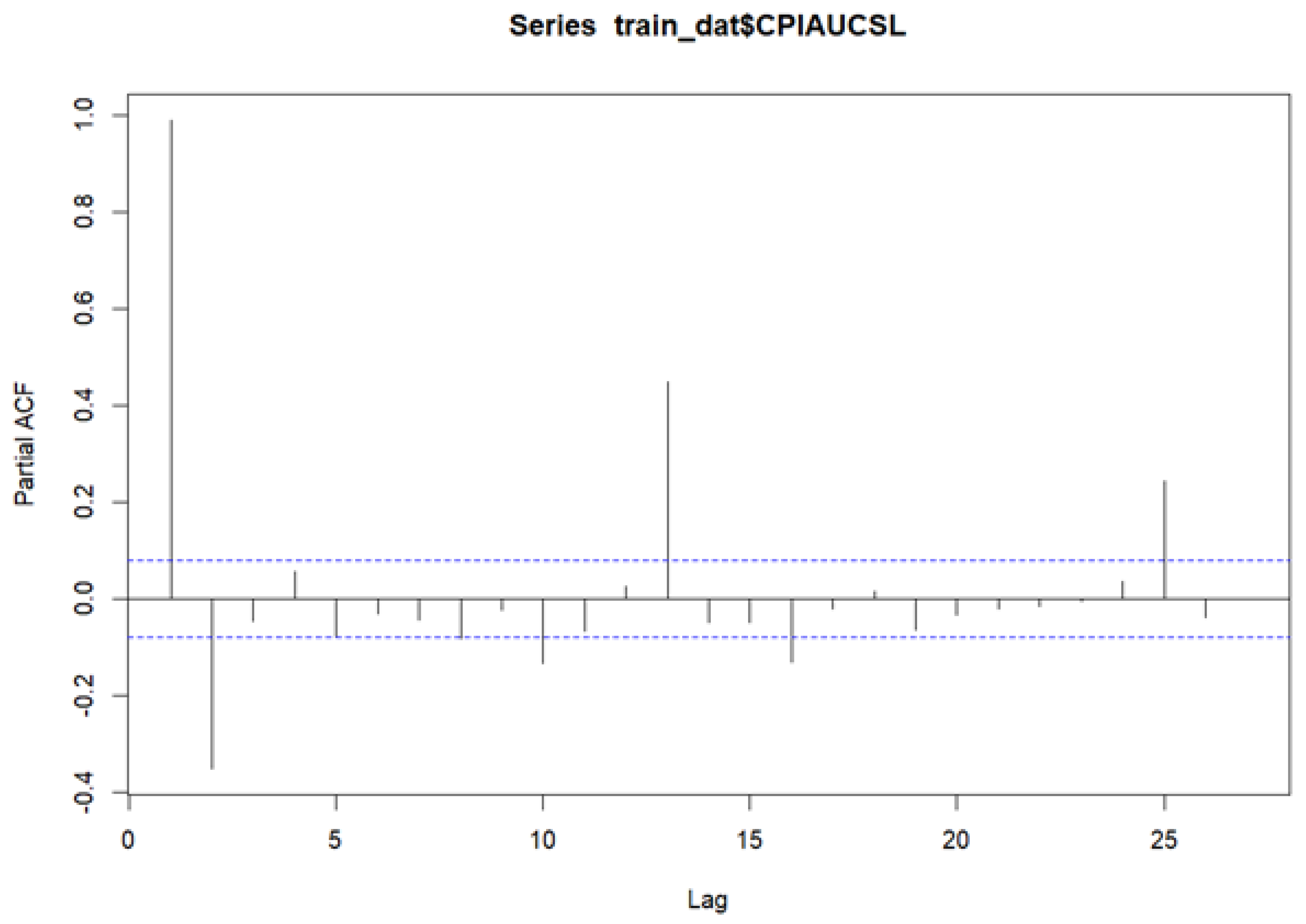
The SARIMA model is built on a linear combination of lagged values and forecast errors. Its effectiveness depends on selecting optimal values for the parameters p, d, and q, which correspond to the autoregressive order, the degree of differencing, and the moving average order, respectively. The differencing order d is chosen to achieve stationarity, typically when the autocorrelation function (ACF) decays to zero. The autoregressive term p is identified by examining the partial autocorrelation function (PACF), where significant spikes beyond the confidence bounds indicate the appropriate lag order.

Equation (2) illustrates the concept of partial autocorrelation, where the response variable y and predictor $x_3$ are adjusted for the effects of intermediate variables $x_1$ and $x_2$. The PAC between y and $x_3$ is defined as the correlation between the residuals from regressing y on $x_1$ and $x_2$, and those from regressing $x_3$ on the same predictors. This isolates the direct linear relationship between y and $x_3$, controlling for the influence of the intervening variables.

$$\begin{array}{cc}\hfill PAC& ={\displaystyle \frac{\mathrm{cov}(\left.y,x_3\right|x_1,x_2)}{\sqrt{\mathrm{var}(y|x_1,x_2)·\mathrm{var}(x_3|x_1,x_2)}}}\hfill \end{array}$$

(2)

The hth order partial autocorrelation can be represented as (3):

$$\begin{array}{cc}\hfill PA{C}^h& ={\displaystyle \frac{\mathrm{cov}(y_i,y_{i-h}|y_{i-h+1},\cdots ,y_{i-1})}{\sqrt{\mathrm{var}(y_i|y_{i-1},\cdots ,y_{i-h+1})·\mathrm{var}(y_{i-h}|y_{i-1},\cdots ,y_{i-h+1})}}}\hfill \end{array}$$

(3)

The q is calculated based on the Autocorrelation (AC) and denotes the error of the lagged forecast:

$$\begin{array}{cc}\hfill AC& ={\displaystyle \frac{{\sum }_{i=1}^{N-k}(y_i-\overline{y})(y_{i+k}-\overline{y})}{{\sum }_{i=1}^N{(y_i-\overline{y})}^2}}\hfill \end{array}$$

(4)

Here,

• $\overline{y}$: The mean of the time series;
• k: The lag, where $k\ge 0$;
• N: The complete series value.

If one requires seasonal patterns in the time series, a seasonal term can be added, which produces a SARIMA model. This model can be written as (5):

$$\begin{array}{c}\hfill ARIMA(p,d,q)\ast (P,D,Q)s(5)\end{array}$$

Here (p, d, q) represent the non-seasonal part, and (P, D, Q) represents the seasonal part of the model. s represents the period number in a season. In this study we employ SARIMA as we assume there exists seasonality in inflation data.

A Seasonal ARIMA (SARIMA) model extends ARIMA by incorporating seasonal differencing at lag s to remove additive seasonal effects, introducing seasonal autoregressive (AR) and moving average (MA) terms. Just as lag-1 differencing removes trends, seasonal differencing addresses cyclical patterns. Seasonal components and lag structures are typically identified through ACF and PACF plots—both at short lags (for non-seasonal terms) and seasonal lags (e.g., 12 months for annual seasonality).

SARIMA is designed for univariate time series with seasonal structure and introduces three additional seasonal parameters (P, D, Q), along with the seasonal period s. It serves as a strong benchmark in inflation forecasting due to its consistent performance. Economic variables like inflation often exhibit seasonality driven by factors such as sales cycles, holidays, or production trends, making SARIMA especially relevant.

Several studies have found that SARIMA frequently outperforms classical models like VAR, AR, and ARIMA, and performs comparably to, or better than, modern machine learning models such as LSTM and feedforward neural networks (Paranhos, 2024). Given its proven effectiveness, SARIMA is used in this study as the primary benchmark against which we evaluate neural network models.

4.5. Benchmark

To assess the performance of the LASSO-LSTM model, we compare it to established benchmarks from the literature: the autoregressive model (AR(p)), seasonal autoregressive integrated moving average (SARIMA), random forest (RF), and LASSO regression. Out-of-sample evaluation is conducted using two forecast periods. For the 2010–2023 period, models are trained on data from 1960 to 2010. For the 1997–2009 period, training data span from 1960 to 1997. Forecast accuracy is measured using root mean squared error (RMSE).

4.6. Network Training

4.6.1. LSTM

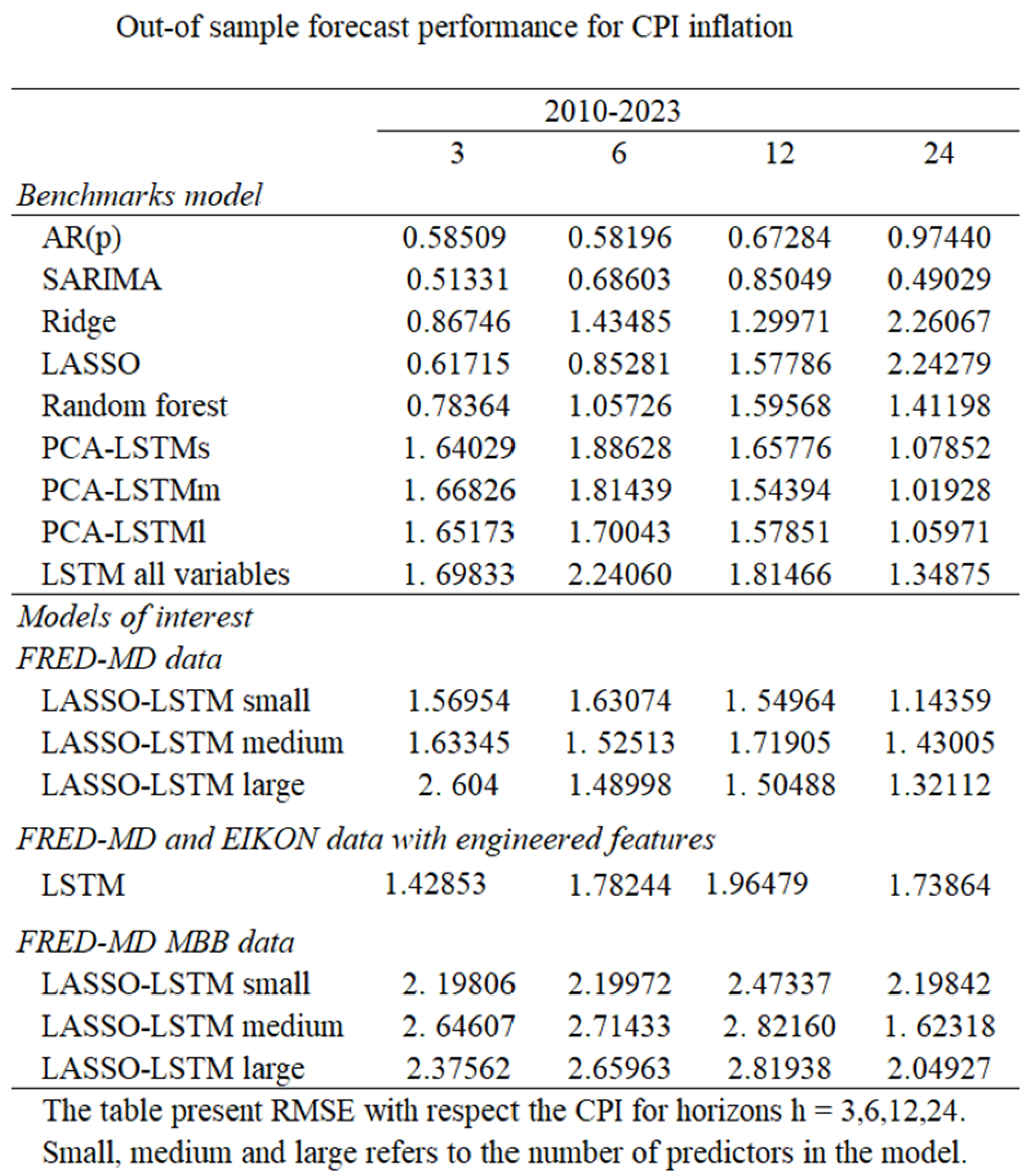
We begin by dividing the dataset into training data, two validation sets, and an out-of-sample test set. The training and validation data span from 1960 to 1997 and are used for model development, while the out-of-sample period ranges from 2010 to the end of 2023.

Model tuning starts with an initial set of hyperparameters used to train the model across thousands of epochs. Each epoch is first evaluated on the initial validation set, and the best-performing epoch is then tested on the second validation set. This tuning process is repeated across multiple hyperparameter combinations. The top-performing epochs from each round are compared using the second validation set, and the best configuration is selected for final testing on the out-of-sample data.

Feature selection is conducted prior to tuning, using both LASSO and PCA, based on the training data and the first validation set. For LASSO-LSTM and PCA-LSTM models, selected features guide input construction.

The specification of the LSTM model consists of four main components:

1. Feature Selection—Relevant variables are identified independently using LASSO or PCA, ensuring dimensionality reduction and interpretability before model training.

2. Model Configuration—This involves defining the model architecture, including lag structure, number and type of layers, dropout rates, and learning rate.

3. Training and Optimization—Training parameters such as the number of epochs, batch size, and validation procedures are set and executed.

4. Model Evaluation—Competing models are evaluated using performance metrics to identify the configuration that generalizes best to unseen data.

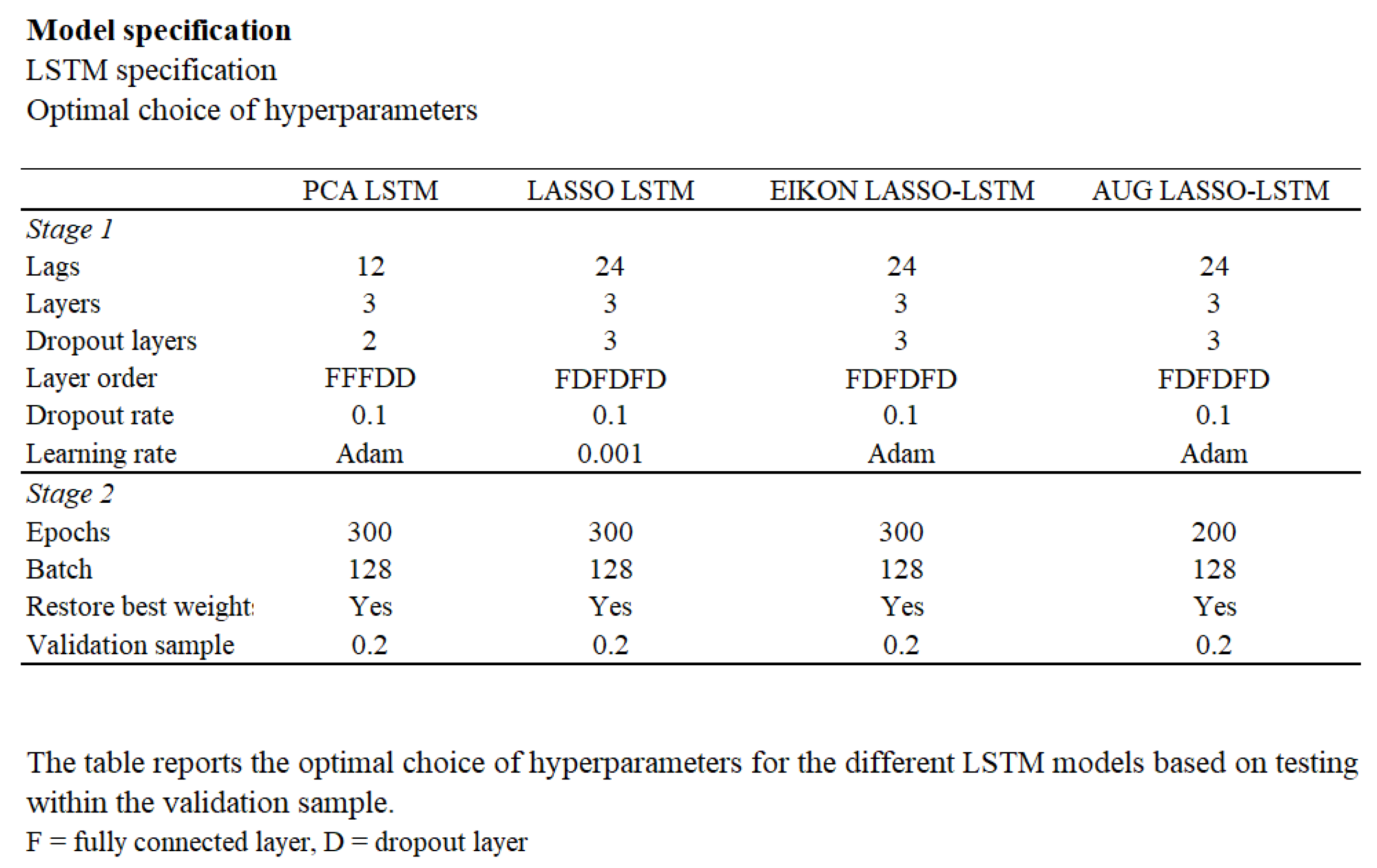
For a summary of model specifications, refer to Figure 6.

4.6.2. Other Machine Learning Models

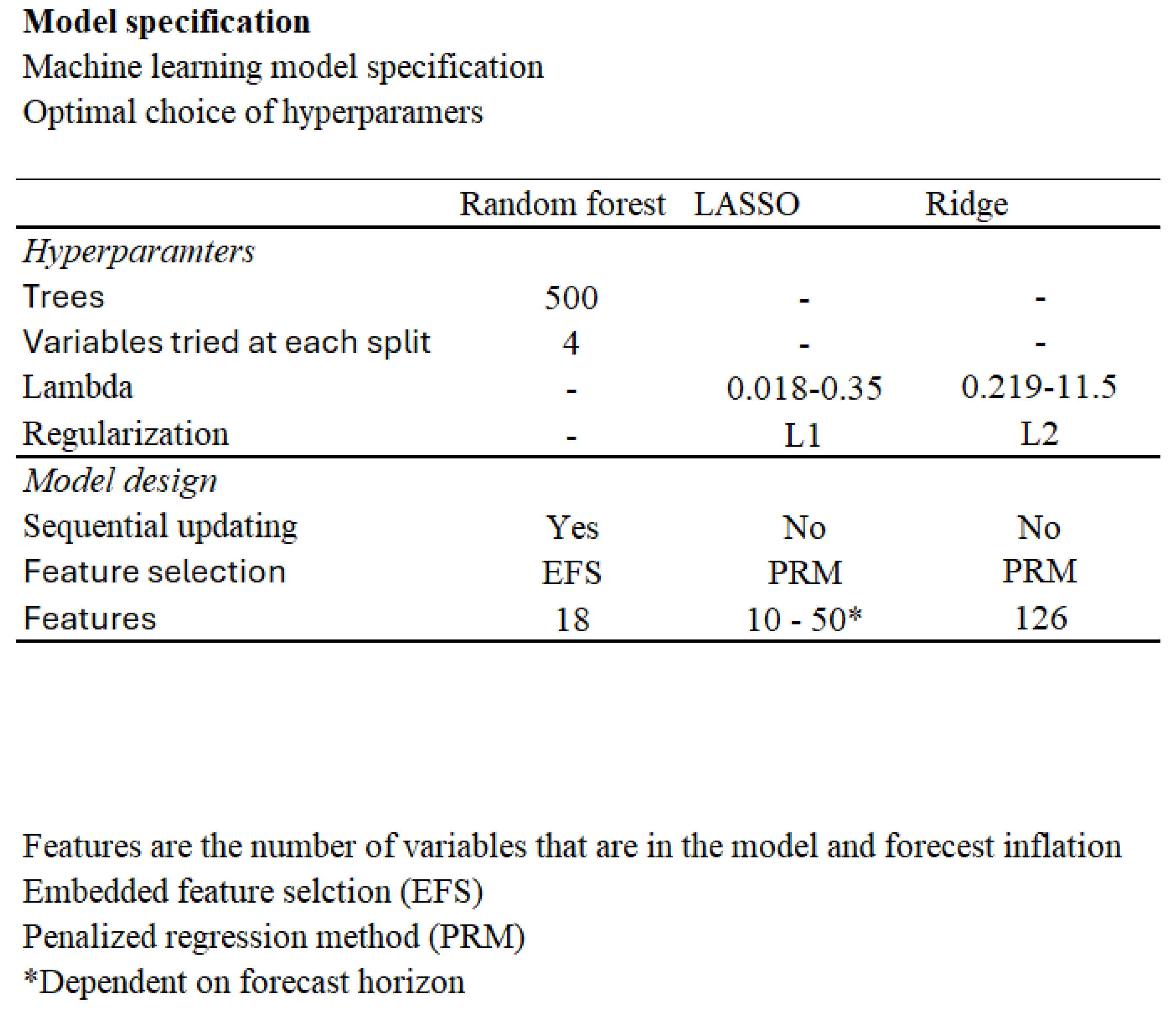
The data used for the remaining machine learning models in this study is divided into three segments: training, validation, and out-of-sample. The period from 1960 to 2010 is reserved for training and validation. An overview of the optimal hyperparameter configurations for each model is provided in Figure 7.

The modeling process begins with embedded feature selection, where predictors are chosen using the training data and validation set. This step is particularly important for the Random Forest algorithm, as it helps identify the most relevant variables before training.

Unlike the other models, Random Forest is implemented with sequential updating, meaning that each forecast incorporates all available data up to the forecast point. As new data becomes available, it is added to the training set, enabling the model to remain responsive to evolving patterns. However, the original feature set and hyperparameters—selected during initial training—remain fixed throughout the forecasting horizon. This setup balances adaptability with consistency, ensuring that the model adjusts to new information while preserving its foundational structure.

LASSO and Ridge regression models follow a similar structure, trained on the training and validation datasets. Their penalty terms are tuned based on performance on the validation sample.

Once optimal configurations are established, all models are evaluated on a reserved out-of-sample dataset to assess their forecasting performance.

4.6.3. Univariate Time Series Models

The specification of the AR(p) model was guided by analyses of the Autocorrelation Function (ACF), Partial Autocorrelation Function (PACF), and the Bayesian Information Criterion (BIC). The SARIMA model was similarly determined using these diagnostics. Both models rely on maximum likelihood estimation, and alternative estimation techniques were not explored. As forecasts are generated, the models are updated sequentially, re-estimating the coefficients while keeping the selected hyperparameters fixed. The optimal hyperparameter configurations for each model are presented in Figure 8.

Sequential Updating Procedure.

All models are evaluated in a real-time forecasting framework using a sequential updating approach. At each time point t, models are retrained on all data available up to t, and forecasts are produced for t + h. As new observations become available, the training window expands accordingly. For the AR(p) and SARIMA models, only the coefficients are re-estimated at each step, while the model orders remain fixed. In the case of LASSO, Ridge, and Random Forest, feature selection and hyperparameters are pre-determined and held constant, with models re-fitted sequentially. LSTM models are retrained at each step using a fixed architecture and consistent hyperparameter settings. This procedure ensures a fair and dynamically updated out-of-sample evaluation across all model types.

4.7. Model Evaluation Methodology

Out-of-sample forecasting performance is assessed using the Root Mean Squared Error (RMSE) across all forecast horizons, comparing predicted values to actual observations. To evaluate the relative performance of each model, results are benchmarked against standard reference models. This comparison provides a basis for assessing the significance and robustness of the forecasting improvements achieved.

5. Results

5.1. Our Approach

In this study, we generate inflation forecasts using a diverse set of models, including univariate time series models, machine learning algorithms, and recurrent neural networks. Benchmark models such as univariate SARIMA, regularized linear regression models (e.g., LASSO), and tree-based methods like Random Forest are applied to the FRED-MD dataset, utilizing various combinations of the 128 available macroeconomic variables. The recurrent neural network model, LSTM, is evaluated using several dataset configurations: FRED-MD alone, FRED-MD combined with EIKON data, and augmented datasets to increase the number of training observations.

All models use a consistent data split, with out-of-sample forecasts covering the period from 2010 to 2023. Forecast horizons range from 1 to 48 months. Due to known initialization challenges, the LSTM model is not validated on the 1-month horizon. We elaborate on this issue in Section 5.5.2. Figure 9 presents RMSE values for each model across the different horizons. These findings are consistent with prior literature (e.g., (Almosova & Andresen, 2023; Paranhos, 2024)), which also reports limited performance gains from LSTM models at short-term horizons.

While our main evaluation metric is RMSE, we refrained from conducting Diebold–Mariano (DM) tests for all model comparisons due to the consistently inferior performance of the LSTM models across all forecast horizons. In these cases, the performance gaps were large and stable across specifications, reducing the incremental value of formal significance testing. Moreover, due to LSTM’s lower interpretability compared to traditional univariate models, it is not meaningful to formally demonstrate the superiority of simpler models in this context.

5.2. Benchmark Model Performance

5.2.1. Univariate Models

Both the AR(p) model and the SARIMA model perform well for all forecasting horizons, reaffirming the existing findings in the literature. For very short and very long forecasting horizons, the SARIMA is superior, while for medium long forecasting horizons, the AR(p) model is the superior performer. The performance of these naive univariate models is superior to most other models for almost all forecasting horizons.

5.2.2. Machine Learning Models

In our study there are three benchmark machine learning models that are used for comparison with the LSTM model. LASSO is superior compared to other machine learning models on a three-month forecasting horizon, and competitive with other models on a 6 month forecast horizon. However as the forecasting horizons increase, the performance of the LASSO model deteriorates showing signs of high bias.

Ridge, the other regularization technique employed in this study, performs similarly to LASSO and achieves good results for short forecast horizons. However, as the horizon increases, the performance of the model deteriorates, showing signs of high bias. This suggests that Ridge will adapt to noise in the model and that shrinking coefficients to zero (Lasso) is a better approach when forecasting. LASSO outperforms the Ridge model for all forecasting horizons, except for the 12-month forecast.

The last machine learning benchmark model is random forest. Figure 10 depicts the random forest 12 months inflation forecast against observed inflation over the same time span. Random forest performs worse than LASSO on short forecast horizons, but displays a more consistent performance all over. While LASSO and Ridge perform poorly for the 24-month forecast horizon, random forest produces competitive results.

5.2.3. PCA-LSTM Performance

The LSTM benchmark models are applied with PCA, where feature selection comes in three forms: LSTM small, LSTM medium, and LSTM large. For shorter forecast horizons, the LSTM models perform poorly compared to the machine learning models and the univariate models. This differs somewhat from findings in the literature, but it is not too surprising since there is not much work on inflation forecasting using LSTM models. Our findings of LSTM on shorter forecasting horizons affirm the need for further studies to determine the ability of neural networks for forecasting inflation. On longer forecasting horizons the LSTM model outperforms other machine learning models, and is partially on par with univariate models. Comparing the three architecture sizes of the LSTM model illustrates that for short to medium forecasting horizons, the differences are negligible.

For longer forecasting horizons the medium sized architecture performs best, which is probably a result of the balance between overfitting and underfitting the model.

5.3. LSTM Model Performance

5.3.1. LASSO-LSTM—FRED-MD Data

The LASSO-LSTM models differ from LSTM in the process of feature selection. Specifically, we examine how LASSO-LSTM performs compared to LSTM, applying the standard PCA feature selection approach.

Results show that for small architectures, the LASSO-LSTM model is able to perform better than the PCA-LSTM model. This is consistent for all horizons except for 24 months ahead, for which PCA-LSTM is marginally better. For medium and large size architectures, there is little difference between the LASSO LSTM and PCA-LSTM. As the number of predictors increases and gets closer to the total number of available predictors, the two models converge in performance.

Among the different LASSO-LSTM models, the smallest architecture is the best performer. It produces superior 3- and 24-month forecasts, but it is slightly outperformed on 6- and 12-month forecasts. The medium architecture is quite consistent for all forecasting horizons but performs worse than the small architecture. The large architecture has some outstanding results, but also some quite poor ones. This is probably due to overfitting. Notably, the large LASSO-LSTM architecture is able to outperform the LSTM model without any feature selection, meaning that any feature selection is better than none. Despite some good forecasts from larger architectures, fewer predictors avoiding overfitting are preferable for inflation forecasting.

Figure 11 illustrates the performance of 6-month inflation forecasts from the LASSO-LSTM model. The model struggles to capture sudden, powerful changes in volatility. The observed under-performance during these volatile periods suggests that while the LASSO-LSTM model is robust in stable conditions, it may need further tuning or additional features to improve its predictive accuracy when the regime in the data changes. This highlights a common challenge in time series forecasting, that models often need to be continuously adapted to handle the complexities of real-world data.

5.3.2. FRED-MD and EIKON Data with Feature Engineering

The reader should recall that a performance summary, in terms of RMSE, is provided in Figure 9. The LSTM model with financial data from the EIKON database and FRED-MD primarily utilizes prices, and performs well on the short forecasting horizon but poorly on longer horizons.

This model utilizes prices and not variables reflecting economic activity. As economic activity is important for longer forecasting horizons, it makes sense that this model performs best for shorter forecasting horizons. Of all LSTM models the financial data LSTM is the best-performing model on the short forecasting horizons.

5.3.3. FRED-MD—MBB Data

The final set of models has undergone a similar feature selection approach as the first set of LASSO-LSTM and utilizes the same dataset. These models only differ because of MBB. The most important model for comparison in this case is the LASSO-LSTM with FRED-MD data. The results related to the data augmented LASSO-LSTM model are quite uninspiring, and the model is not able to deliver superior results at any forecasting horizon for any size of architecture. Thus, data augmentation as an attempt to increase training data was unsuccessful. The model training time also increases considerably compared to all other LSTM models. Presumably, the augmented data does not retain the sequence well enough and is ineffective in capturing different regimes and other patterns in macroeconomic data.

5.4. Benchmarks Versus LSTM-Type Models

While demonstrating an improvement in performance when switching from PCA to LASSO feature selection, LSTM is still not able to deliver competitive forecasts compared to the univariate time series models. For shorter forecasting horizons there are other machine learning models, such as LASSO, that are able to provide better forecasts than LSTM. Random forest is also better at shorter forecast horizons. As forecast horizons increase, LSTM forecasts improve. The LSTM model is better than all of the machine learning models for the 24-month forecast, and quite good for 12-month forecasts. All other machine learning models show signs of high bias in their 24 months forecasts. However, this issue was not possible to solve during specification on the validation sample, as LASSO and random forest did not improve when features were removed or added. This indicates that the LSTM model could be a good option compared to other machine learning models on longer forecast horizons.

5.5. Theoretical Considerations Why LSTM Models May Struggle in Forecasting Inflation

5.5.1. Data Constrains

A primary limitation in applying LSTM models to macroeconomic forecasting is the scarcity and quality of available data. LSTM networks are data-intensive, requiring substantial datasets to effectively learn temporal patterns. However, macroeconomic indicators are typically reported at monthly or quarterly intervals, resulting in relatively small datasets. Moreover, data quality prior to 1960 is often inconsistent, further constraining the training process.

Additionally, the relationship between inflation and its predictors is inherently complex and non-linear. While LSTM models are adept at capturing non-linear patterns, they assume a degree of stationarity in these relationships. In practice, macroeconomic relationships are subject to structural changes over time, leading to non-stationarity that can challenge the model’s predictive capabilities. Recent studies have highlighted that while LSTM models can outperform traditional models in certain contexts, their performance may degrade when faced with such non-stationary data patterns.

Macroeconomic variables often exhibit structural breaks and evolving relationships over time. When blocks from different periods are recombined, as in the Moving Block Bootstrap (MBB), there is a risk of inadvertently mixing distinct economic regimes or contexts, which can distort underlying trends and dynamics. Consequently, caution is warranted when applying MBB in settings where preserving the temporal sequence and regime integrity is crucial.

5.5.2. Forecast Horizon and Model Complexity

Our findings indicate that LSTM models tend to perform better over longer forecasting horizons, particularly during periods of heightened macroeconomic uncertainty. This aligns with recent research suggesting that LSTM models can capture long-term dependencies more effectively than some traditional models. However, for shorter horizons, simpler models like LASSO regression or SARIMA often yield more accurate forecasts. This inconsistency complicates the recommendation of LSTM models for general forecasting purposes.

Furthermore, LSTM architectures are inherently complex, involving multiple layers and a wide range of hyperparameters, which makes them challenging to configure and fine-tune. This complexity not only increases the computational cost but also presents significant obstacles to reproducibility and transparency, both of which are essential considerations for policymakers and applied researchers. The “black-box” nature of LSTM models limits their interpretability, thereby making it more difficult to extract clear, actionable insights—a well-documented drawback in the context of economic forecasting.

Gradient Instability and Vanishing Gradients: Although LSTMs were designed to mitigate the vanishing gradient problem found in vanilla RNNs, they are still susceptible to gradient instability in long sequence learning. This can result in difficulties when learning long-term dependencies, which are critical in capturing inflation dynamics driven by persistent economic shocks.

In closing this discussion, we note that we exclude LSTM models from the 1-month ahead forecast horizon due to severe initialization instability and inconsistent performance across multiple training runs. These issues likely stem from the limited temporal dependencies present at such short horizons, which make LSTM’s sequence-based architecture less effective. While this decision improves the robustness of the reported results, it does limit comparability across models at the shortest forecast horizon—a particularly relevant time frame for monetary policy applications, including inflation forecasting. We acknowledge this as a limitation of the current study and encourage future research to explore alternative LSTM configurations, ensemble methods, or architecture tuning strategies that may yield more reliable performance in short-term forecasting contexts.

5.6. Future Research

Recognizing the limitations noted above, future research may benefit from exploring hybrid approaches that combine the predictive capabilities of LSTM models with the transparency and interpretability of traditional econometric techniques. Alternatively, research could focus on identifying or developing neural network architectures that are more aligned with the structural characteristics and constraints of macroeconomic data.

To enhance the accuracy of inflation forecasting models, future research should further focus on advanced data augmentation techniques that preserve the inherent properties of time series data, such as regime shifts and random walk characteristics. Implementing methods like MBB can help maintain autocorrelation structures within the data, leading to more robust model training. Integrating LASSO regularization into LSTM networks has shown promise in improving model performance by effectively handling high-dimensional datasets and preventing overfitting. Additionally, exploring ensemble approaches that combine LASSO with tree-based models, such as Random Forests, can leverage the strengths of both methods to capture complex patterns in inflation data.

While ensemble models offer potential performance gains, it is important to consider the balance between model complexity and interpretability. Tree-based models and penalized regression techniques, like LASSO, often provide more transparent insights, which are valuable for policymakers. Although current LSTM models may underperform compared to simpler alternatives, advancements in recurrent neural networks (RNNs) could enhance their applicability in macroeconomic forecasting.

Furthermore, investigating other neural network architectures, such as Convolutional Neural Networks (CNNs) and Transformers, may yield valuable insights due to their ability to capture both local and global dependencies in time series data.

6. Conclusions

This study evaluated the effectiveness of LSTM models in forecasting U.S. inflation, comparing their performance against traditional time series models such as SARIMA and AR(p), as well as machine learning approaches like LASSO regression. While integrating LASSO for feature selection enhanced LSTM performance, the LSTM models generally underperformed compared to simpler models across most forecasting horizons.

Notably, LSTM models showed relative strength in longer-term forecasts. However, their complex architecture, which includes numerous layers and hyperparameters, poses challenges in model tuning and reproducibility. Additionally, the “black box” nature of LSTM models limits interpretability, a crucial factor for policymakers and central bankers who require transparent and explainable forecasting tools.

Data limitations may contribute to the subpar performance of LSTM models in this context. Macroeconomic data, such as inflation indicators, are typically reported at monthly or quarterly intervals, resulting in relatively small datasets. Furthermore, the data encompasses unique economic events—including shifts in central bank policies, the Global Financial Crisis, and the COVID-19 pandemic—which introduce complex, non-stationary relationships that are challenging for LSTM models to capture effectively.

While LSTM models are capable of modeling non-linear patterns, their performance is hindered when these non-linearities evolve over time. In contrast, simpler models like LASSO regression, AR(p), and SARIMA have demonstrated more consistent and reliable performance in inflation forecasting, making them more suitable for practical applications in economic policy and decision-making.

In terms of interpretability, incorporating LASSO for feature selection within LSTM models (LASSO-LSTM) has provided clearer insights into variable importance, as LASSO emphasizes significant predictors while diminishing the influence of less relevant ones. This approach not only enhances model transparency but also contributes to improved forecasting accuracy, as evidenced by lower RMSE values.

In conclusion, while LSTM models offer potential advantages in modeling complex, non-linear relationships, their current limitations, particularly in data-scarce environments, suggest that simpler, more interpretable models like LASSO regression, AR(p), and SARIMA remain more practical and effective for inflation forecasting. Advancements in data augmentation and hybrid modeling approaches may, however, enhance the applicability of LSTM models in future macroeconomic forecasting endeavors.