Sustainable Factor Augmented Machine Learning Models for Crude Oil Return Forecasting

Abstract

The global crude oil market, known for its pronounced volatility and nonlinear dynamics, plays a pivotal role in shaping economic stability and informing investment strategies. Contrary to traditional research focused on price forecasting, this study emphasizes the more investor-centric task of predicting returns for West Texas Intermediate (WTI) crude oil. By spotlighting returns, it directly addresses critical investor concerns such as asset allocation and risk management. This study applies advanced machine learning models, including XGBoost, random forest, and neural networks to predict crude oil return, and for the first time, incorporates sustainability and external risk variables, which are shown to enhance predictive performance in capturing the non-stationarity and complexity of financial time-series data. To enhance predictive accuracy, we integrate 55 variables across five dimensions: macroeconomic indicators, financial and futures markets, energy markets, momentum factors, and sustainability and external risk. Among these, the rate of change stands out as the most influential predictor. Notably, XGBoost demonstrates a superior performance, surpassing competing models with an impressive 76% accuracy in direction forecasting. The analysis highlights how the significance of various predictors shifted during the COVID-19 pandemic. This underscores the dynamic and adaptive character of crude oil markets under substantial external disruptions. In addition, by incorporating sustainability factors, the study provides deeper insights into the drivers of market behavior, supporting more informed portfolio adjustments, risk management strategies, and policy development aimed at fostering resilience and advancing sustainable energy transitions.

1. Introduction

Fluctuations in international crude oil market prices are closely linked to the development of the global economy and social stability. As a unique commodity, crude oil prices and investment returns are primarily driven by supply and demand dynamics (Wang & Hao, 2023). However, crude oil is also affected by irregular factors, including weather conditions, inventory levels, GDP growth, political factors, psychological expectations, and increasingly sustainability-related considerations such as environmental regulations and the global energy transition. Consequently, this volatility offers traders and investors opportunities to profit from price fluctuations. As Baur and Lucey (2009) point out, during economic turmoil or uncertainty, crude oil can serve as a hedge against increased financial market stress. Additionally, crude oil is essential for national economic development and maintaining global economic and financial stability (Dong et al., 2018). Thus, the forecasting of crude oil, driven by these factors, has attracted significant interest from institutions, business practitioners, and researchers, establishing it as a crucial field of study.

In recent years, the growing emphasis on sustainable development has significantly influenced the analysis of energy markets. International frameworks such as the United Nations Sustainable Development Goals underscore the urgent need for affordable and clean energy, responsible resource management, and effective climate change mitigation (Sachs et al., 2024). Accurate prediction of crude oil prices plays a critical role in advancing these objectives. Reliable forecasts enable policymakers and market participants to better anticipate price volatility, optimize resource allocation, and design strategies that support energy affordability and security. Moreover, effective oil price forecasting contributes to more stable and transparent markets, which are essential for guiding investment towards cleaner technologies and facilitating the transition to sustainable energy systems. In this context, improving the predictability of crude oil prices is important not only for financial decision making but also for achieving broader sustainability outcomes.

How can crude oil returns be predicted more accurately? The literature identifies two main methodological approaches. Traditional econometric models, such as ARIMA, GARCH, and vector autoregressive models, are effective for relatively stable time series but often struggle to capture the high volatility and complex dynamics present in crude oil markets (Wang & Fang, 2022). As a result, the recent studies increasingly employ machine learning methods, including random forest, XGBoost, long short-term memory, and multilayer perceptrons, which are better suited to modeling the nonlinear relationships characteristic of financial time series with significant fluctuations (Dixon et al., 2017). However, most of the existing research has not sufficiently integrated a broad range of influential variables, particularly those related to sustainability and external risks. Given that crude oil is affected by macroeconomic trends, financial market conditions, and policy changes (Álvarez-Díaz, 2020), the challenge of accurate forecasting persists. Incorporating a more comprehensive set of relevant factors into forecasting models is therefore crucial for further enhancing predictive accuracy (Guo et al., 2023).

This study’s main contributions are as follows. First, it provides an empirical basis for forecasting crude oil investment returns rather than prices, thereby directly supporting investor decision making and expanding the scope of crude oil futures analysis (Niu et al., 2022). Second, through a systematic comparison of both linear and nonlinear forecasting models, this study identifies the most effective approach for crude oil futures prediction (Jiang et al., 2022; Lin & Su, 2021). Third, by incorporating a comprehensive set of 55 predictors across five major categories, the research offers a broader perspective than previous studies that were limited to a narrow set of indicators (Shin et al., 2013). Fourth, the results indicate that the inclusion of sustainability and external risk factors, such as ESG indicators, carbon prices, and global risk shocks, leads to significant improvements in the accuracy of WTI crude oil return forecasts, underscoring the importance of these variables. Fifth, the analysis quantifies the individual contribution of each variable, thereby enhancing model interpretability and transparency, which is essential for effective risk management (Lundberg & Lee, 2017). Sixth, the proposed model demonstrates superior predictive accuracy and performance compared to previous financial time-series studies, providing a more reliable reference for investors. Finally, the study reveals that the COVID-19 pandemic has fundamentally altered the dynamics and key drivers of crude oil investment returns, offering new insights into the impact of special events on financial markets (Peng & de Moraes Souza, 2024).

In summary, this study addresses three key deficiencies in the current research. First, prior studies often overlook return forecasting and have a limited focus on high volatility markets, leading to an insufficient understanding of investor-oriented metrics. Second, the existing approaches rarely integrate such a broad range of potential predictors. We improve upon this by fusing multiple factors and systematically comparing diverse machine learning methods. Third, empirical applications often lack full transparency or interpretability around key predictive variables, which is crucial for policy and risk management. Using SHAP and performing extensive sensitivity checks, our findings can inform policymakers and practitioners about which drivers matter and how market disruptions like COVID-19 alter predictive dynamics. It demonstrates that our study not only achieves higher predictive accuracy and shows tangible profit potential in trading simulations. The practical value of our findings lies in supporting both short term and strategic decision making for investors and policy planners, not only by providing more accurate return forecasts for hedging and allocation but also by enhancing transparency and supporting regulatory efforts aimed at fostering more resilient and sustainable energy markets. By accounting for sustainability and external risks, our approach equips policymakers to better anticipate and manage disruptions, thereby contributing to the broader objectives of global energy transition and climate resilience. The ability to better anticipate market responses to sustainability-related risks and opportunities can facilitate more resilient energy policies, accelerate the adoption of cleaner technologies, and strengthen the financial system’s capacity to support the global energy transition. As such, our findings not only advance the literature on return predictability but also provide an actionable framework for aligning investment and policy decisions with the broader imperatives of sustainable development.

The structure of the remaining sections of this paper is as follows: Section 2 reviews the relevant literature. Section 3 introduces the selected predictive models and evaluation metrics. Section 4 details the variable selection mechanisms used in this study and provides descriptive statistics. Section 5 analyzes the results of the forecasting. Section 6 provides the conclusion of the paper.

2. Literature Review

2.1. Mechanisms Influencing Crude Oil Futures

The dynamics of crude oil futures prices have long been a central topic in energy economics. Early research predominantly focused on the supply and demand balance theory. For example, Kilian categorized crude oil price fluctuations as either supply or demand shocks (Kilian, 2009). He argued that demand shocks, particularly those from global economic activity, primarily drove price increases. However, the pronounced price swings since 2007, such as the 2008 crash from 145.29 to 33.87 per barrel in five months, reveal the limitations of this traditional framework. These extreme events illustrated that the supply and demand model alone is insufficient to explain the heightened volatility that characterizes modern crude oil markets. They also drew attention to the increasing influence of speculative activities in shaping crude oil futures prices.

With the rise of financialization in energy markets, speculative trading played a more prominent role in driving oil price movements. Masters observed that oil pricing has grown more dependent on futures market dynamics, with global financial actors including hedge funds, investment banks, and speculators playing pivotal roles (Masters, 2009). Kilian and Murphy provided empirical evidence that speculative demand, rather than just physical supply and demand, accounted for a substantial portion of oil price volatility during key periods (Kilian & Murphy, 2014). This finding is echoed by Juvenal and Petrella, who demonstrated that speculative activities tended to amplify price fluctuations (Juvenal & Petrella, 2011). Gogolin and Kearney further emphasized the critical role of futures market mechanisms in driving these dynamics (Gogolin & Kearney, 2016). However, the literature still lacks clarity on how financialization and speculation interact with market fundamentals. This gap indicates a need for more integrative models.

In recent years, research has increasingly highlighted the impact of external uncertainties on crude oil futures prices. Macroeconomic conditions, policy changes, and geopolitical risks have all emerged as significant factors. Ma et al. improved forecasting accuracy by adding economic policy uncertainty (EPU) to predictive models (Ma et al., 2018). This result highlights the importance of policy-driven risks. Mei et al. showed that geopolitical risk uncertainty can enhance short-term volatility forecasting, suggesting that sudden political events often lead to sharp oil price fluctuations (Mei et al., 2020). Li et al. extended this line of inquiry by incorporating indices such as policy uncertainty, trade uncertainty, and geopolitical risk into WTI crude oil volatility forecasts, which confirmed the relevance of these external factors (Li et al., 2022). Additionally, Thomas et al. found that during extreme price surges, commodities such as gold, silver, and agricultural products, along with currency pairs like USD/EUR and USD/GBP, showed strong correlations with crude oil (Conlon et al., 2024). These findings underscore the increasingly complex and interconnected nature of crude oil markets.

In general, the evolution of the crude oil futures pricing mechanisms reflects a shift from reliance on traditional fundamentals to a more multifaceted system shaped by financialization and a broad array of external risks. This complexity challenges the explanatory power of classical models and highlights the pressing need for more sophisticated and adaptive forecasting methodologies. Despite important advances, there are still gaps in understanding the dynamic interplay between these diverse factors, especially under conditions of structural market change or external crises.

2.2. Crude Oil Price Forecasting Methodology

The increasing complexity of crude oil price dynamics, shaped by both fundamental and speculative influences, has highlighted the need for more robust and adaptive forecasting frameworks. Traditional econometric models, such as GARCH and ARCH, have been widely employed for crude oil price forecasting because of their ability to capture time-varying volatility. For example, it has been shown that GARCH models outperform simple random walk models in predicting WTI crude oil prices (Sadorsky, 2006), while enhanced ARCH models can effectively capture the volatility characteristics of both WTI and Brent crude oil prices (Cheong, 2009). Nevertheless, these models are often constrained by strict assumptions, including stationarity, linearity, and normally distributed residuals, which limit their capacity to address the inherently complex, non-linear, and non-stationary nature of crude oil price series (Bahrammirzaee, 2010). Furthermore, their reliance on predefined functional forms makes them less adaptable to rapidly changing market conditions and structural breaks.

To overcome these limitations, computational intelligence and machine learning techniques have gained increasing attention in the field of financial time-series forecasting. Unlike traditional models, machine learning approaches are capable of extracting non-linear and non-stationary patterns from data without imposing rigid distributional assumptions. For instance, dynamic model averaging (DMA) has been utilized to examine the impact of interest rates and exchange rates on INE crude oil prices, achieving superior accuracy compared to traditional methods (Lin & Su, 2021). It has also been found that integrating long short-term memory (LSTM) networks with investor sentiment indices can improve prediction accuracy for Chinese crude oil prices by capturing long-term dependencies in the data (Jiang et al., 2022). In addition, attention mechanisms and graph-based neural networks (GWNet) have been applied to WTI crude oil price forecasting, revealing that macroeconomic variables such as the US Dollar Index, LIBOR, and VIX have become increasingly influential, sometimes surpassing the predictive power of traditional supply and demand factors (Zhao et al., 2023).

Recent developments in hybrid and deep learning models further underscore the advantages of machine learning in handling the multifaceted spatial and temporal relationships present in crude oil markets. For example, the MTGNN-TAttLA model, which integrates graph neural networks (GNNs) with attention mechanisms, has been used to capture spatial dependencies among influencing factors while prioritizing the most impactful variables (Foroutan & Lahmiri, 2024). This approach achieved state-of-the-art forecasting performance, demonstrating the adaptability and accuracy of hybrid architectures in complex financial settings. For example, Stasiak et al. (2025) developed state models based on a binary–temporal representation to support short-term crude oil price forecasting and demonstrated their effectiveness through multi-year backtests with high-frequency data and practical trading system implementation (Stasiak et al., 2025).

In summary, machine learning methods overcome the limitations of traditional econometric models by capturing nonlinear, nonstationary, and complex dependencies in crude oil price data. With advanced techniques such as attention mechanisms and graph neural networks, these approaches integrate diverse information sources and adapt to changing market conditions, resulting in more accurate and robust forecasts in the increasingly complex crude oil market.

2.3. Impact of Pandemics on the Oil Market

The COVID-19 pandemic has created unprecedented disruptions in the crude oil market, fundamentally reshaping price dynamics and exposing new forms of vulnerability. Early empirical studies documented a substantial increase in oil price volatility closely tied to pandemic-related news and uncertainty. For example, heightened sensitivity of oil prices to pandemic developments has been identified (Narayan, 2020), while the formation of price bubbles as demand collapsed under the pressure of lockdowns and global mobility restrictions has also been noted (Gharib et al., 2021).

The research has also revealed that the pandemic deepened the interconnectedness between oil and financial markets. Significant volatility spillovers from oil to broader financial systems have been found, contributing to escalating global economic uncertainty (Albulescu, 2020). Further studies have highlighted that disruptions in industrial production and transportation led to profound supply–demand imbalances, aggravating price volatility and exposing the market’s susceptibility to systemic shocks (Bai et al., 2021). These findings suggest that traditional approaches, which often treat oil prices in isolation, may fail to capture the full extent of market vulnerability during global crises.

In response to these challenges, the recent literature has increasingly emphasized the value of advanced forecasting methodologies. Machine learning models, particularly those employing attention mechanisms and LSTM networks, have demonstrated superior performance in modeling the complex, non-linear, and rapidly evolving patterns characteristic of pandemic-induced market behavior (Tian et al., 2023). It has also been shown that integrating high-frequency macroeconomic indicators, policy announcements, and real-time news sentiment into these models leads to more accurate and adaptive forecasts.

However, much of the current literature continues to rely on a limited range of predictors, often neglecting the ways in which key market characteristics evolve in response to significant disruptions such as the pandemic. There has also been relatively little attention paid to the integration of variables that capture the specific impacts of pandemic-related developments. Broadening the analytical framework to incorporate these shifting features and additional relevant factors may yield a more comprehensive understanding of oil price dynamics under conditions of heightened uncertainty.

3. Methodology

3.1. Forecasting Model

In selecting the forecasting model (see

Table 1. Overview of Forecasting Models.

Model	Strengths	Applicability
OLS	Computationally efficient; effective for capturing linear relationships	Benchmark; linear relationship assessment
XGBoost	Powerful nonlinear modeling; sensitive to complex feature interactions	Multi-factor, complex relationship modeling
Random Forest	Strong noise resistance; stable performance with high dimensional data	Multi-variable, noisy data scenarios
BP	Capable of fitting complex nonlinear patterns; highly flexible architecture	Basic nonlinear modeling
MLP	Supports multi-dimensional input; deep feature learning capability	Multi-factor driven forecasting
CNN	Excels at extracting local temporal features; effective for short term fluctuations	High frequency volatility
LSTM	Strong ability to model long term dependencies and capture temporal trends	Long term trend, inertia modeling

), this study takes into account the high volatility and nonlinear characteristics inherent in financial time series, as well as the need to model multidimensional variables. Traditional linear models offer advantages in terms of interpretability and capturing simple linear relationships. However, they struggle to maintain strong predictive performance in highly nonlinear financial markets with complex interactions. To address these limitations, we have chosen a diverse set of nonlinear machine learning models, which are better suited to capturing intricate patterns, modeling variable interactions, and improving predictive accuracy in dynamic financial environments, and include a linear regression model for comparative analysis.

3.1.1. Ordinary Least Squares (OLS)

Ordinary Least Squares (OLS) regression is a widely used method for estimating the parameters of a linear model. The fundamental idea is to minimize the sum of squared differences between the observed and predicted values. For a given linear model,

$$y={\beta }_0+{\beta }_1{x}_1+{\beta }_2{x}_2+\cdots +{\beta }_p{x}_p+ϵ$$

(1)

where y represents the dependent variable, $x_1,x_2,\dots ,x_p$ are the independent variables, ${\beta }_0,{\beta }_1,\dots ,{\beta }_p$ are the parameters to be estimated, and $ϵ$ is the error term.

OLS achieves parameter estimation by minimizing the following objective function:

$$\mathrm{minimize}\sum _{i=1}^n{(y_i-{\widehat{y}}_i)}^2$$

(2)

where ${\widehat{y}}_i$ is the predicted value from the model.

3.1.2. Extreme Gradient Boosting (XGBoost)

Extreme gradient boosting (XGBoost) is an enhancement of the gradient boosting machine, developed by Chen and Guestrin (2016). It improves prediction accuracy by constructing a series of decision trees. Combining the contributions of all the trees, the final prediction model is as follows:

$${\widehat{y}}_i=\sum _{k=1}^K{f}_k\left(x_i\right)$$

(3)

where ${\widehat{y}}_i$ is the predicted value for the i-th instance. K represents the total number of trees in the model, $f_k$ is the function representing the k-th tree, and $x_i$ is the feature vector of the i-th instance.

3.1.3. Random Forest

Random forest is an ensemble learning algorithm that aggregates the predictions of multiple decision trees built on randomly sampled subsets of the data, which enhances predictive accuracy and robustness for both regression and classification tasks (Breiman, 2001). Its fundamental formula is as follows:

$$\widehat{Y}={\displaystyle \frac{1}{q}}\sum _{i=1}^q{g}_k\left(X\right)$$

(4)

where $\widehat{Y}$ represents the output of the model, X is the input feature vector, and q denotes the number of trees. $g\left(X\right)$ is a set of k-th learner random trees.

3.1.4. Convolutional Neural Network (CNN)

Convolutional neural networks (CNNs) are feedforward neural networks that utilize convolutional layers to automatically extract local features from data. In financial time-series forecasting, CNNs effectively capture important short-term patterns and temporal structures within input sequences (Haykin, 2009). A one-dimensional convolutional layer can be defined as follows:

$$S\left(t\right)=\sum _{m=0}^{M-1}X(t-m)·F\left(m\right)$$

(5)

where X represents the input time series, F is the convolutional kernel, M is the size of the kernel, m is the position index within the convolution kernel, and $S\left(t\right)$ is the output feature at time t.

3.1.5. Backpropagation Neural Network (BP)

The backpropagation neural network (BP) is a classic multilayer feedforward neural network trained using the error backpropagation algorithm, allowing it to effectively model complex non-linear relationships in data.

The core formulas are as follows:

$$E={\displaystyle \frac{1}{2}}\sum {(\widehat{y}-y)}^2$$

(6)

where E is the error function, y represents the actual output, and $\widehat{y}$ is the predicted output of the network.

Weight update:

$$\Delta w=-\eta {\displaystyle \frac{\partial E}{\partial w}}$$

(7)

$$w_{\mathrm{new}}=w_{\mathrm{old}}+\Delta w$$

(8)

where $\eta$ is the learning rate, and w represents the network’s weights.

3.1.6. Multilayer Perceptron (MLP)

A multilayer perceptron (MLP) is a feedforward neural network composed of an input layer, one or more hidden layers, and an output layer. Its flexible architecture allows it to approximate complex nonlinear functions, making it effective for a wide range of prediction tasks (Haykin, 2009).

3.1.7. Long Short-Term Memory (LSTM)

Long short-term memory (LSTM) networks are an advanced form of recurrent neural networks that utilize memory cells and gating mechanisms to effectively capture long-term dependencies in sequential data, making them particularly suitable for time-series prediction tasks (Hochreiter & Schmidhuber, 1997). The core formulas are

$$\begin{array}{cc}\hfill f_t& =\sigma (W_f·[h_{t-1},x_t]+b_f)\hfill \end{array}$$

(9)

$$\begin{array}{cc}\hfill i_t& =\sigma (W_i·[h_{t-1},x_t]+b_i)\hfill \end{array}$$

(10)

$$\begin{array}{cc}\hfill o_t& =\sigma (W_o·[h_{t-1},x_t]+b_o)\hfill \end{array}$$

(11)

$$\begin{array}{cc}\hfill C_t& =f_t\ast C_{t-1}+i_t\ast tanh(W_C·[h_{t-1},x_t]+b_C)\hfill \end{array}$$

(12)

$$\begin{array}{cc}\hfill h_t& =o_t\ast tanh\left(C_t\right)\hfill \end{array}$$

(13)

where $f_t$, $i_t$, $o_t$ represent the activation values of the forget gate, input gate, and output gate, respectively; $C_t$ is the cell state; $h_t$ is the output value; W and b are the weight and bias parameters; and $\sigma$ is the sigmoid activation function.

3.2. Assessment Metrics

Selecting appropriate evaluation metrics is essential in machine learning to accurately assess and determine the best-performing models. We have selected three metrics types, including error metrics, coefficient of determination, and accuracy. These metrics provide a comprehensive reference for evaluating the predictive performance of our model and are instrumental in guiding the optimization process.

3.2.1. Error Metrics

We employ standard error-based evaluation metrics, including mean squared error (MSE), root mean squared error (RMSE), and mean absolute error (MAE), to assess model predictive accuracy. These metrics quantify the average magnitude of prediction errors and are widely used in regression analysis. The calculation processes for these metrics are as follows:

$$\begin{array}{cc}\hfill \mathrm{MSE}& ={\displaystyle \frac{1}{n}}\sum _{i=1}^n{(y_i-{\widehat{y}}_i)}^2\hfill \end{array}$$

(14)

$$\begin{array}{cc}\hfill \mathrm{RMSE}& =\sqrt{{\displaystyle \frac{1}{n}}\sum _{i=1}^n{(y_i-{\widehat{y}}_i)}^2}\hfill \end{array}$$

(15)

$$\begin{array}{cc}\hfill \mathrm{MAE}& ={\displaystyle \frac{1}{n}}\sum _{i=1}^n|y_i-{\widehat{y}}_i|\hfill \end{array}$$

(16)

where $y_i$ represents the observed values, ${\widehat{y}}_i$ is the predicted value, and n is the number of samples. Lower values in these three metrics signify reduced error, indicating improved model predictive accuracy.

3.2.2. Coefficient of Determination ($R^2$)

The coefficient of determination ($R^2$) is used to measure the proportion of the variance in the dependent variable that the independent variables can explain. This metric assesses the explanatory power of the model. Its calculation process is as follows:

$$\begin{array}{c}\hfill R^2=1-{\displaystyle \frac{{\sum }_{i=1}^n{(y_i-{\widehat{y}}_i)}^2}{{\sum }_{i=1}^n{(y_i-\overline{y})}^2}}\end{array}$$

(17)

where $\overline{y}$ is the average of the observed values, $y_i$ represents the actual outcomes, ${\widehat{y}}_i$ is the predicted outcome from the model, and n is the number of samples.

3.2.3. Directional Accuracy (DA)

Directional accuracy (DA) is a metric used to evaluate how accurately a model forecasts the direction of data changes. It can be calculated using the following formula:

$$\begin{array}{c}\hfill DA={\displaystyle \frac{1}{N}}\sum _{i=1}^N\mathbf{1}(\mathrm{sign}({\widehat{y}}_i-y_{i-1})=\mathrm{sign}(y_i-y_{i-1}))\end{array}$$

(18)

where N is the total number of observations, and $\mathbf{1}$ is an indicator function that equals 1 when the predicted direction of change matches the actual direction of change and 0 otherwise.

4. Data

This study, we focus on identifying the best method to predict WTI returns accurately. We integrated insights from the prior research and introduced new features not previously considered that could theoretically influence WTI returns.

4.1. Dependent Variable

In this study, the dependent variable is the weekly returns of WTI. We gathered WTI futures price data from invest.com, covering the period from 1 January 2001 to 31 March 2024 and used these to calculate the weekly returns. In daily data, market noise can arise from factors such as irrational behaviors of market participants and short-term fluctuations in market sentiment. In contrast, weekly returns minimize the impact of single-day extremes and short-term volatility, stabilizing overall trend analysis. By aggregating data at the weekly level, short-term anomalies are smoothed out, which not only reduces the risk of model overfitting but also enhances the robustness and reliability of the prediction results.

4.2. Independent Variable

(1)

Macro-economic independent variables

The significance of macroeconomic variables in predicting WTI crude oil returns primarily lies in their ability to provide comprehensive information about economic activities, consumer behavior, and policy environments. These elements significantly influence the supply and demand dynamics and price fluctuations in the crude oil market. The previous research has extensively leveraged macroeconomic variables to analyze and forecast energy prices and returns, including crude oil. For instance, Kilian (2009) identified global macro-economic conditions as one of the key factors affecting oil prices. Additionally, Hamilton (2009) emphasized how macroeconomic factors are instrumental in explaining fluctuations in oil prices. From this, we choose the following variables:

GDP, capacity utilization (CU), real disposable personal income: per capita (RDPI), unemployment rate (Unrate), industrial production index (IPI), consumer price index (CPI), population (POP), Chicago Fed’s National Activity Index (CFNAI), money supply (MS), global economic policy uncertainty (GEPU).

(2)

Financial markets’ independent variables

The study by Kilian and Murphy (2014) demonstrates that financial variables, such as stock market indices and interest rates, significantly influence crude oil price forecasts. These variables provide direct insights into market sentiment, investor behavior, and changes in macroeconomic policies. They also considerably influence capital flows and investment decisions. Consequently, we have selected the following variables:

Bond yield (BYD), interest rate (IR), S&P Goldman Sachs Commodity Index (GSCI), USD/EUR, USD/JPY, USD/QAR, USD/SAR, VIX Panic Index (VIX), treasury rate (TR), NASDAQ Index (NASDAQ), Treasury Bond 30-Year Yield (TBY30), Treasury Bond 10-Year Yield (TBY10), Treasury Bond 2-Year Yield (TBY2), S&P500 (S&P 500), Dow Jones Industrial Average Index (DJIA), Barrick Gold Corporation Stock (BGCS), gold price (Gold), silver price (SL), Shanghai Composite Index (SHCI), Tadawul Index (Tadawul), soybean price (SB), Bull.

(3)

Energy markets’ independent variables

Energy market variables are critical in economic models and market analysis because they provide essential insights into the interactions between energy demand, supply, pricing, and economic activity (Hamilton, 2009). These variables directly reflect the supply and demand conditions of crude oil, and the prices and availability of many crude oil substitutes also serve as fundamental factors influencing crude oil prices. For this mechanism, we have selected the following variables:

Per Capita Oil Consumption Index (OSI), Crude Oil Contribution to GDP (OCI), Kilian’s Index (Kilian), CSI Energy Index (EI), Brent Index (Brent), natural gas price (NG), S&P Energy (SPE), growth of crude oil production (COP), fuel oil price (FO).

(4)

Momentum independent variables

To investigate the effectiveness of the direction momentum variables in predicting of price movements, this study defines some momentum variables related to our target markets. Our choices of momentum variables are based on prior studies on the effect of momentum variables in predicting crude oil or precious metals prices (Shin et al., 2013). We have selected the following variables:

Rate of change (ROC), Relative Strength Index (RSI), and three exponential moving averages (EMA): signal line, moving average convergence/divergence (MACD), and triple exponential moving average (TEMA).

(5)

Sustainability and external risk

Incorporating sustainability and external risk variables into crude oil return forecasts enables an investigation into whether models can better capture not only sudden disruptions but also underlying, long-term shifts associated with the global transition toward low-carbon development. As the world accelerates efforts in climate policy, green finance, and adoption of clean technologies, these sustainability trends change the patterns of energy demand and investment (International Energy Agency, 2023; Wu et al., 2023; Yin et al., 2023). Ignoring such factors may lead to incomplete or biased forecasts, especially as sustainability considerations increasingly influence market behavior and capital flows (Mukhtarov et al., 2022). By systematically introducing sustainability into crude oil forecasting for the first time, this study provides a more accurate and forward-looking perspective. This approach enhances predictive performance while offering valuable insights into how ongoing sustainability transitions and external shocks jointly shape the dynamics of crude oil markets.

Epidemic risk index (ERI), natural disaster count (Count), Green Bond rate (GBR), carbon price index (CP), ESG index (ESG), electric vehicle sales (EVS).

4.3. Descriptive Statistics

4.3.1. Summary Statistics

In this study, we conducted a comprehensive descriptive statistical analysis of WTI crude oil returns from 2000 to 2024. This analysis assesses the time-series characteristics of the data, providing a foundation for training machine learning models. As shown in

Table 2. Descriptive statistics of WTI return.

Year	Mean	Std	Min	Median	Max	Skewness	Kurtosis
2000	0.0016	0.0533	−0.1264	0.0044	0.1683	−0.1550	0.9616
2001	−0.0032	0.0534	−0.1969	−0.0014	0.0959	−1.1938	2.8476
2002	0.0092	0.0463	−0.1103	0.0052	0.1018	−0.1658	0.0740
2003	0.0009	0.0535	−0.1996	0.0074	0.0951	−1.1760	2.9042
2004	0.0035	0.0471	−0.1381	0.0076	0.1208	−0.2901	0.5825
2005	0.0076	0.0392	−0.0788	0.0079	0.0879	−0.1946	−0.5928
2006	0.0029	0.0294	−0.0576	0.0006	0.0651	0.0749	−0.9903
2007	0.0084	0.0390	−0.0894	0.0138	0.1046	−0.3153	0.3232
2008	−0.0162	0.0628	−0.1618	0.0005	0.1838	−0.2033	0.8943
2009	0.0174	0.0736	−0.1942	0.0057	0.2226	0.2469	1.2526
2010	0.0062	0.0382	−0.1153	0.0105	0.0653	−0.8398	0.6681
2011	0.0037	0.0442	−0.1260	0.0091	0.0827	−0.5673	0.6378
2012	−0.0026	0.0266	−0.0780	0.0017	0.0600	−0.4219	0.4933
2013	0.0021	0.0242	−0.0409	0.0037	0.0620	0.2604	−0.3363
2014	−0.0119	0.0309	−0.1162	−0.0118	0.0332	−1.0790	1.9790
2015	−0.0052	0.0570	−0.1137	−0.0027	0.2283	1.1190	3.2694
2016	0.0085	0.0553	−0.1313	0.0102	0.1141	−0.1328	−0.5375
2017	0.0038	0.0337	−0.0904	−0.0003	0.0838	−0.0495	0.3323
2018	−0.0043	0.0404	−0.1345	−0.0022	0.0844	−0.6378	0.8218
2019	0.0051	0.0396	−0.0925	0.0053	0.1078	−0.1593	0.0787
2020	−0.0584	0.3476	−1.8444	0.0082	0.4249	−4.2272	19.7811
2021	0.0099	0.0393	−0.0939	0.0088	0.0920	−0.3182	0.3595
2022	0.0064	0.0641	−0.1140	0.0012	0.2524	0.8147	2.4789
2023	−0.0009	0.0419	−0.1072	−0.0049	0.1007	0.2553	−0.0889
2024	0.0067	0.0303	−0.0593	0.0090	0.0589	−0.5277	1.1529
ALL	−0.0002	0.0843	−1.8444	0.0040	0.4249	−13.0085	274.8975

Note: ALL indicates the statistics for the entire sample period.

, the average annual return of WTI from 2000 to 2024 exhibited slight fluctuations, with the highest annual return of 1.74% in 2009 and the lowest at −5.84% in 2020. This significant drop primarily reflects the turbulence in the global economic environment that year, mainly due to the market uncertainties triggered by the COVID-19 pandemic.

The standard deviation, a measure of price volatility, peaked at 34.76% in 2020, underscoring the instability of WTI returns for that year. The extreme range between the minimum and maximum values, notably −184.44% to 42.49% in 2020, also highlights the exceptional market volatility. Analysis of skewness and kurtosis reveals that WTI returns typically showed a slight negative skew in most years, indicating a distribution slightly biased towards negative returns. Kurtosis was generally close to or below the standard distribution value of 3. Still, in specific years like 2020, it soared to 19.78, indicating an unusually thick tail in the distribution of returns, a sign of extreme market instability.

Summarizing the statistics for the entire period (2000–2024), the average weekly return was nearly zero (–0.02%), indicating a long-term stabilization of WTI returns. However, the overall standard deviation of weekly returns was 8.43%, with a skewness of –13.01 and a kurtosis reaching 274.90, revealing the potential for extreme market conditions during specific periods. All statistics reported here are based on weekly return data.

At the same time, we focused on the ten independent variables that have the most important crucial effect on WTI crude oil price returns. As shown in

Table 3. Descriptive statistics of Top 10 important independent variables.

Variables	Mean	Std	Min	Median	Max	Kurtosis
ROC	−0.017	8.433	−184.439	0.396	42.494	274.898
VIX	20.040	8.531	9.313	17.953	79.750	7.407
CFNAI	−0.127	1.111	−18.120	−0.053	6.260	103.796
USD/SAR	3.751	0.003	3.706	3.750	3.770	114.472
USD/QAR	3.642	0.006	3.634	3.641	3.734	67.340
CPI	0.212	0.357	−1.915	0.211	1.374	3.531
GSCI	4093.234	1605.104	1281.427	3892.687	10,701.200	1.098
SHCI	2593.630	867.682	1013.660	2705.100	5987.813	0.545
RSI	53.057	17.270	0.736	54.097	97.881	−0.016
NG	4.468	2.218	1.551	3.846	14.665	2.455

, the most critical of these variables was the rate of price change (ROC), which demonstrated substantial volatility and extreme values. This variable’s mean was close to zero (−0.017), indicating that the average ROC in WTI crude oil prices was negligible throughout the study period. However, with a standard deviation of 8.433, it also showed high price volatility. The minimum and maximum values were −184.439 and 42.494, respectively, revealing significant price drops and spikes. Additionally, the skewness of the rate of price change was −13.008, indicating a highly asymmetric distribution that leaned left, suggesting that significant price declines were more prominent than rises during the observation period. The kurtosis was 274.898, significantly higher than a normal distribution, indicating a prevalence of extreme values.

Another significant predictor, the VIX, shows a standard deviation of 8.531, reflecting moderate to high market uncertainty. The distribution is moderately right-skewed, indicating occasional spikes in market volatility.

Other variables such as CFNAI, USD/SAR, USD/QAR, CPI, GSCI, SHCI, RSI, and NG provide additional insights into the macro-economic and market-specific factors influencing WTI returns. Each variable, with its distinct statistical characteristics, contributes uniquely to the predictive model, enhancing the accuracy and robustness of the return forecasts.

4.3.2. Time Trend

Figure 1 illustrates the weekly returns on WTI crude oil from 1 January 2020, to 31 March 2024. The figure highlights significant fluctuations in the return during this period. Notably, there was an extraordinary decline in early 2020, where the return rate plummeted to below $-1.5$. This sharp drop reflects the profound impact of the global COVID-19 pandemic on the oil market.

4.3.3. Correlation Test

Figure 2 presents a Spearman correlation matrix between the returns of WTI crude oil and several key indicators. This heatmap not only reveals the strength of associations among the indicators but also visually displays the direction of correlations through variations in color intensity. The correlation between WTI returns and the S&P GSCI (GSCI) index is the highest at 0.48, while correlations with other variables are relatively lower, such as 0.24 with the rate of change (ROC), 0.13 with CPI, and 0.08 with both VIX and RSI. Both ROC and the relative strength index (RSI), two technical indicators, show higher correlations with WTI returns than most other variables. Among other features, some variables exhibit strong correlations, with the highest being between GSCI and natural gas (NG) at 0.76. The most notable negative correlation is between GSCI and USD/SAR at −0.46.

5. Results

5.1. Forecast Results in 4 Week Rolling

We adopt a rolling window strategy with a 4-week window to forecast WTI returns, training the model on the most recent 4 weeks of data at each step. Input features are constructed by lagging daily variables by 1 week and monthly variables by 4 weeks, so that only information available prior to the forecast period is used. To further ensure temporal alignment and data consistency, monthly variables are interpolated to a weekly frequency before being lagged, so that each week is assigned a unique, smoothly evolving value for these features. This interpolation avoids abrupt step-wise changes, better reflects the gradual evolution of economic indicators, and allows the model to capture macroeconomic trends more realistically. This rolling window design allows the model to systematically update with the latest available data, ensuring that each prediction reflects prevailing market conditions and relies solely on historical information, thus mitigating information leakage or forecast bias and contributing to the robustness of the results. In addition, by incorporating lagged features, the model is able to capture temporal dependencies and evolving patterns commonly observed in financial time series. This approach not only aligns forecasts with current market dynamics but also simulates an out-of-sample setting at every step, further reducing the risk of information leakage. From an economic perspective, this methodology reflects the adaptive nature of financial markets, where agents continually update their beliefs and strategies based on new information, and past behaviors can influence future prices through mechanisms such as momentum, mean reversion, and delayed information diffusion. As a result, our approach helps mitigate look-ahead bias, reduces the risk of overfitting, and naturally provides an out-of-sample evaluation with each forecast.

Given the sensitivity of OLS to multicollinearity, we addressed this issue by applying principal component analysis (PCA) to the predictor variables prior to model fitting. PCA transforms the original potentially correlated features into a set of orthogonal principal components, thereby reducing multicollinearity and improving the reliability of OLS estimates. In addition, for all models, including OLS and more complex models, all input features were standardized to have zero mean and unit variance. This standardization ensures comparability between models and enhances convergence and stability during training, especially for algorithms that are sensitive to the scale of input variables.

To assess the contribution of sustainability and external risk variables, we first conducted model training and prediction without these variables, and subsequently repeated the process with their inclusion. As presented in

Table 4. Forecast results in 4 week rolling (without sustainability and external risk variables).

Model	MSE	${\mathit{R}}^2$	MAE	RMSE	Accuracy
OLS	0.0053	0.2550	0.0360	0.0728	0.5523
XGBoost	0.0055	0.2350	0.0128	0.0742	0.7468
Random Forest	0.0063	0.1200	0.0334	0.0794	0.5887
CNN	0.0065	0.1100	0.0388	0.0806	0.5662
BP	0.0066	0.0700	0.0396	0.0812	0.5464
MLP	0.0061	0.1300	0.0375	0.0781	0.5625
LSTM	0.0063	0.1150	0.0368	0.0794	0.5548

and

Table 5. Forecast results in 4 week rolling (with sustainability and external risk variables).

Model	MSE	${\mathit{R}}^2$	MAE	RMSE	Accuracy
OLS	0.0047	0.3442	0.0331	0.0682	0.5650
XGBoost	0.0048	0.3242	0.0113	0.0693	0.7643
Random Forest	0.0057	0.1941	0.0308	0.0756	0.5987
CNN	0.0059	0.1759	0.0361	0.0787	0.5741
BP	0.0059	0.1274	0.0369	0.0787	0.5529
MLP	0.0055	0.2232	0.0348	0.0743	0.5721
LSTM	0.0057	0.1940	0.0342	0.0756	0.5628

, the addition of these variables resulted in consistent performance improvements across all models. For instance, the accuracy of XGBoost increased from 0.7468 to 0.7643, with parallel enhancements observed in other metrics such as MSE and MAE. These findings suggest that sustainability and external risk variables offer substantial informational value, enabling models to deliver more accurate and robust predictions. This improvement can be attributed to the fact that sustainability and external risk factors encapsulate underlying economic, environmental, and market dynamics that exert direct or indirect influence on financial outcomes. By integrating these variables, the models are able to capture a broader spectrum of risks and opportunities, thereby enhancing their capacity to discern complex patterns and adapt to evolving conditions within financial markets.

After incorporating all variables associated with the mechanism, the predictive performance of the models was further evaluated. As shown in Table 5, we compared the linear model (OLS) with five nonlinear models (XGBoost, RF, CNN, BP, MLP, and LSTM). The OLS model presented MSE, MAE, RMSE, and ACC values of 0.0047, 0.3442, 0.0331, 0.0682, and 0.5650, respectively. In contrast, the non-linear XGBoost model showed MSE, MAE, RMSE, and ACC values of 0.0048, 0.3242, 0.0113, 0.0693, and 0.7643, respectively. XGBoost exhibited superior performance across all metrics, particularly in accuracy, where it was approximately 20% higher than that of OLS. Furthermore, XGBoost’s MAE of 0.0113, significantly lower than that of OLS at 0.0331, indicates more precise error control. Among all models compared, XGBoost performed the best, not only achieving the highest accuracy rate of 76.43% and demonstrating strong predictive performance across other key metrics. These results underscore XGBoost’s efficiency and reliability in capturing complex nonlinear patterns and handling large datasets, making it a robust choice for financial prediction tasks.

5.2. Model Interpretation

In this section, we employ the Shapley Additive exPlanations (SHAP) method to interpret the model. Developed from the principles of game theory, SHAP values are a powerful tool to measure the contribution of each variable towards the prediction outcome (Lundberg & Lee, 2017). High precision models, such as ensemble models and deep learning models, feature complex and variable internal structures that are not intuitively understandable. However, SHAP, a classical post hoc explanation framework, can calculate the importance value of each feature variable in every sample, thereby achieving an explanatory effect. The advantage of this method lies in its ability to provide insights into both the local and global behaviors of the model, which is crucial for confirming the reliability and performance of dynamic models within the volatile environments of financial markets.

Using the best performing XGBoost model as an example, we utilized SHAP to assess and output the top 10 variables important for predicting WTI return rates, as illustrated in Figure 3. The right side displays the SHAP values for each feature within the model, where each dot represents a variable’s contribution to the model output in a given instance. Positive SHAP values (pink dots) indicate that higher variable values tend to increase the predicted returns, whereas negative values (blue dots) suggest a decrease in returns. On the left, the average of the absolute values of SHAP for each variable is shown; the more significant the value, the greater the average influence of the variable within the model. Among these variables, rate of change (ROC) stands out as the most important predictor, exhibiting the highest mean absolute SHAP value. Notably, ROC demonstrates large SHAP values in both positive and negative directions, with substantial color variability, indicating a broad range of impacts on the model predictions. This suggests that ROC plays a pivotal role in shaping the model’s output under different market conditions. The strong influence of ROC aligns with economic theory, as it reflects momentum shifts in asset prices, which are widely used by traders and analysts to gauge market sentiment and potential trend reversals.

In financial market analysis, ROC is a key momentum indicator that helps identify potential buy or sell signals. It is particularly valuable in volatile markets like crude oil, where price fluctuations occur rapidly. The high SHAP value of ROC underscores its ability to capture short-term market dynamics, allowing the model to adapt swiftly to changing conditions. Moreover, the bidirectional impact of ROC, as seen in the SHAP analysis, highlights its role in both upward and downward price movements, reinforcing its significance in technical analysis and trading strategies.

As shown in

Table 6. Results of variable importance.

	OLS	XGBoost	Random Forest	CNN	BP	MLP	LSTM
1	ROC	ROC	ROC	ROC	ROC	ROC	ROC
2	CFNAI	CFNAI	VIX	VIX	VIX	VIX	VIX
3	OSI	VIX	CFNAI	CFNAI	CFNAI	CFNAI	CFNAI
4	CPI	USD/SAR	USD/SAR	USD/SAR	USD/SAR	USD/SAR	USD/SAR
5	GSCI	USD/QAR	USD/QAR	USD/QAR	USD/QAR	USD/QAR	USD/QAR
6	EMA_5	CPI	CPI	CPI	CPI	CPI	CPI
7	GEPU	GSCI	GSCI	GSCI	GSCI	GSCI	GSCI
8	VIX	USD/EUR	SHCI	SHCI	SHCI	SHCI	SHCI
9	UNRAT	RSI	RSI	RSI	RSI	RSI	RSI
10	COP	NG	NG	NG	NG	NG	NG

, we compare the rankings of feature importance across seven different machine learning models in predicting WTI returns. Since the ordinary OLS model cannot utilize SHAP values, we assess the significance of each coefficient in the model using statistical measures (T-values). Significant differences exist between linear (OLS) and nonlinear models (including XGBoost, Random Forest, CNN, BP, MLP, and LSTM) in identifying key variables. In addition to differing in evaluation methods, OLS, as a linear model, solely focuses on the direct linear relationships between features and the target variable, ignoring any interactions or nonlinear relationships. Consequently, the features it identifies as necessary may differ from those other models recognize.

In contrast, nonlinear models can capture complex nonlinear relationships and better handle interactions and pattern recognition among variables.

Furthermore, the deep learning models such as CNN, BP, MLP, and LSTM share the same top ten important features, likely due to their strong capabilities in data representation and abstraction, which results in a higher dependency on similar features. Random forest and the deep learning models display identical feature rankings, and the top ten essential variables in the XGBoost model are also highly similar to those in the deep learning models. This indicates that these variables exhibit strong predictive signals or significant statistical correlations, contributing substantial explanatory power to the models.

The results show that various nonlinear models significantly emphasize variables such as ROC, VIX, CFNAI, USD/SAR, USD/QAR, and CPI. Notably, ROC is the most crucial feature in all models, highlighting its key role in predicting WTI returns due to price momentum. VIX, CFNAI, and CPI also receive high ranks, emphasizing their strong influence on oil investment returns through market volatility and macroeconomic activities. The significance of USD/SAR and USD/QAR in predicting WTI returns is primarily linked to the roles of Saudi Arabia and Qatar in the global energy market. As major oil-exporters, these nations experience exchange rate fluctuations that may influence their oil production and export decisions, thereby impacting WTI investment returns.

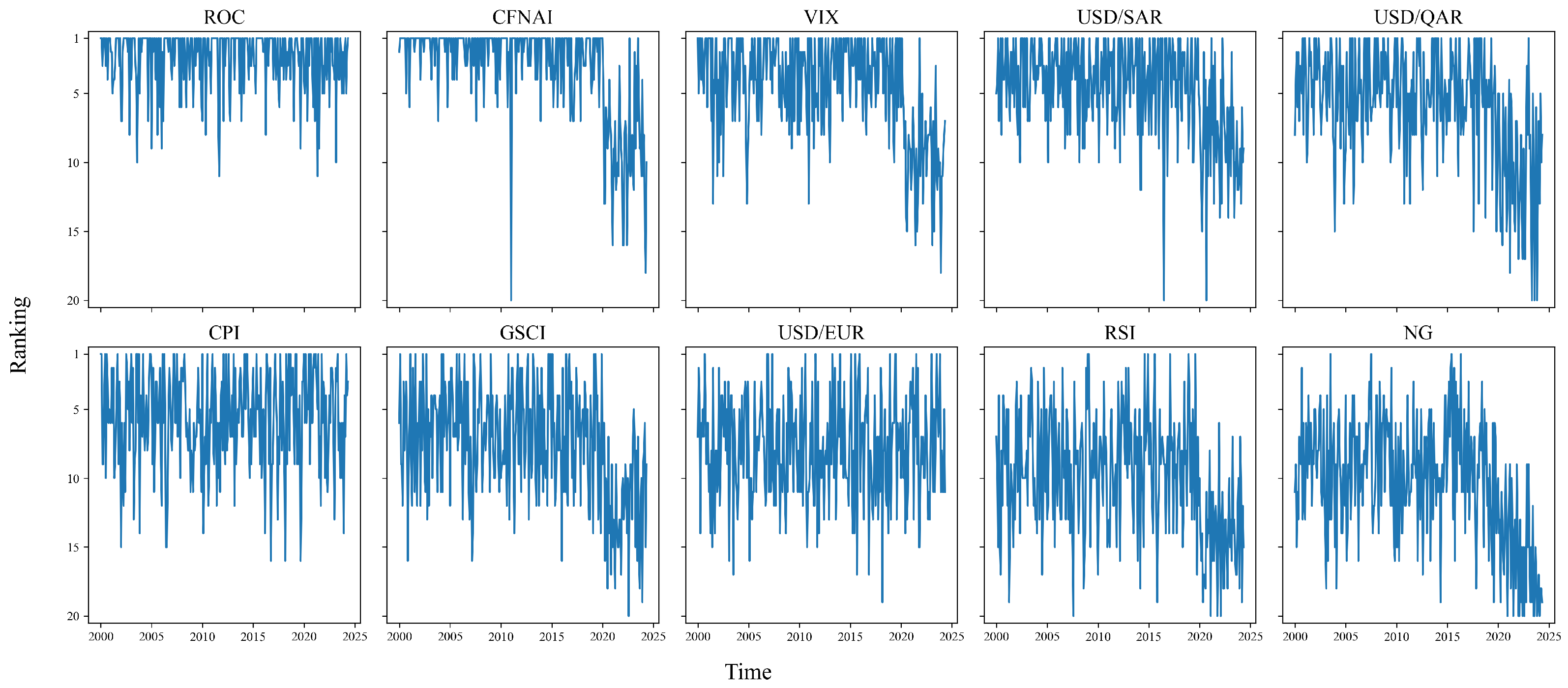
In addition to the aggregated importance rankings, it is also instructive to examine how the importance of these variables evolves over time. Figure 4 displays the dynamic ranking trajectories of the top 10 features identified by XGBoost, where lower values on the vertical axis correspond to higher importance. Each subplot traces the ranking of a specific variable across the full sample period.

The plots reveal several important patterns. First, ROC consistently maintains the highest importance, with its ranking rarely dropping below the top few positions, which further corroborates its central role in the predictive modeling of WTI returns. Other macroeconomic and financial indicators, such as CFNAI, VIX, USD/SAR, and USD/QAR, also maintain relatively high rankings throughout most of the sample but show notable declines in importance during and after the COVID-19 period—reflecting structural changes in market dynamics and the relative informativeness of different features in turbulent times. In contrast, variables like CPI and USD/EUR display more stable ranking trajectories, indicating that their predictive contributions remain relatively constant over time.

This dynamic perspective on feature importance is particularly valuable in the context of financial time series forecasting, where market regimes and the relationships among variables can change rapidly over time. By tracking the ranking trajectories of each variable across rolling forecast windows, we provide clear evidence that the predictive roles of even the most important features are not fixed, but can shift significantly with evolving economic conditions or major events such as the COVID-19 pandemic. This approach enables us to identify periods when certain variables become especially influential or, conversely, lose their predictive power, which may signal underlying changes in market structure or investor behavior. As a result, practitioners can use such insights to adjust their trading and risk management strategies proactively, ensuring that models remain relevant and robust in the face of ongoing market changes.

5.3. Strategy Validation

(1)

Validity

To evaluate the practical application of machine learning models, this study develops a trading strategy based on model predictions and calculates its capital curve under scenarios with and without transaction fees. When transaction fees are not considered, positions are determined based on the model’s weekly returns prediction: long positions are taken when the predicted return is above zero, short positions are taken when it is below zero, and no positions are held when the prediction is zero. Profits or losses are calculated weekly based on these positions. The total cumulative return since the strategy’s inception is ultimately determined by aggregating these weekly net profits or losses. The strategy’s effectiveness is demonstrated using a simulated capital curve, starting with an initial capital of 1. The equity curve is calculated with the following formula:

$$\begin{array}{c}\hfill \mathrm{Capital}\mathrm{Curve}=\mathrm{initial}\mathrm{capital}+\mathrm{cumulative}\mathrm{return}\end{array}$$

(19)

This equity curve reflects the trajectory of capital changes when an investor starts with an initial capital of 1 and invests according to the machine learning model strategy.

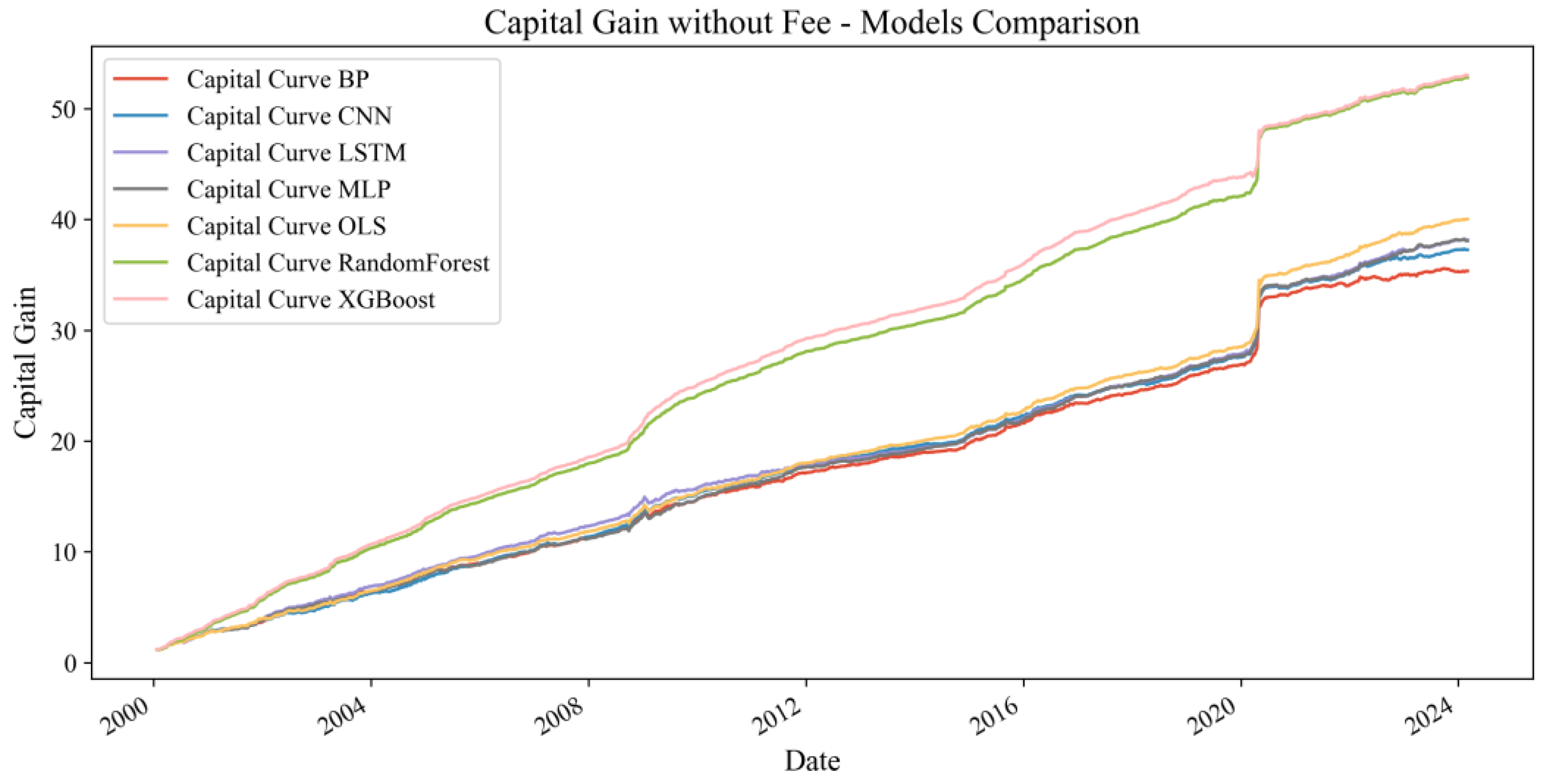
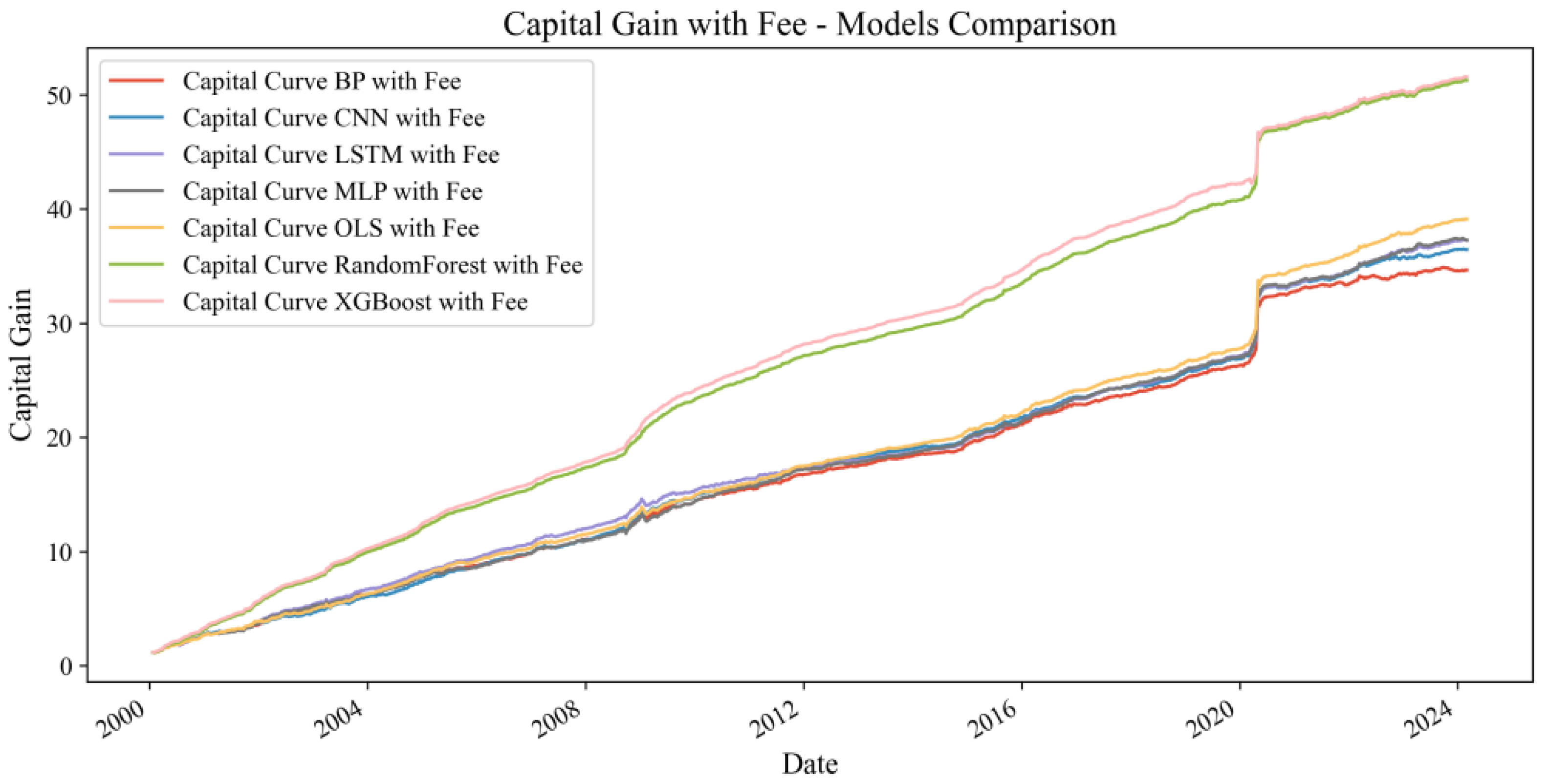
When transaction fees are considered and the initial capital is set at 1, a fee of 5% of the initial capital, or 0.05, is deducted for calculating net profits or losses. This fee adjustment is then applied to calculate the cumulative return and capital curve. As shown in Figure 5, accounting for transaction costs, all model capital growth curves demonstrate annual increases from 2000 to 2024, emphasizing the strategic advantage of machine learning models in predicting crude oil investment returns. Notably, the XGBoost model maintains a higher level of capital growth, significantly outperforming others and indicating robust strategy effectiveness even with trading costs. As illustrated in Figure 6, excluding transaction costs improves all model returns, yet the XGBoost model maintains a clear advantage. This underscores the efficiency and practicality of the XGBoost model in forecasting WTI crude oil returns.

Table 7. Performance comparison of different models.

Model	AR	AR-Fee	SR	SR-Fee	MDD	MDD-Fee	Vol	Vol-Fee
OLS	16.20	16.10	1.67	1.65	−10.8	−11.2	38.3	38.1
XGBoost	17.10	17.05	2.10	2.08	−7.4	−8.0	37.9	37.8
Random Forest	16.80	16.70	1.88	1.86	−12.2	−13.0	39.2	39.1
CNN	15.95	15.90	1.60	1.58	−18.5	−19.2	40.8	40.6
BP	16.40	16.32	1.74	1.72	−16.0	−16.5	40.2	40.0
MLP	16.10	16.05	1.61	1.59	−13.8	−14.1	40.1	39.9
LSTM	15.20	15.15	1.45	1.44	−38.6	−39.0	47.5	47.4

Note: AR = annualized return (%), SR = Sharpe ratio, MDD = max drawdown (%), Vol = annualized volatility (%); “-Fee” denotes with transaction costs.

presents the comprehensive performance metrics for all evaluated models. The results show that all machine learning models, including traditional OLS, achieve relatively high annualized returns and Sharpe ratios, which demonstrates their effectiveness in predicting crude oil returns. Among all models, the XGBoost model exhibits the strongest overall performance. It achieves the highest annualized return, reaching 17.10% without transaction fees and 17.05% with transaction fees. In addition, XGBoost records the highest Sharpe ratio at 2.10 without fees and 2.08 with fees. Its maximum drawdown is also the lowest among all models, at −7.4% without fees and −8.0% with fees, indicating better risk control and more stable performance. Furthermore, the annualized volatility of XGBoost remains at a relatively low level (37.9% without fees and 37.8% with fees), which further supports its risk-adjusted advantage.

Other models, such as OLS, random forest, BP, MLP, and CNN, also deliver solid results. They all generate annualized returns and Sharpe ratios that are only slightly lower than those of XGBoost. However, these models tend to experience higher maximum drawdowns and volatility, which suggests that their risk management capability is not as strong as that of XGBoost. In contrast, the LSTM model, although it achieves a reasonable annualized return of 15.20% (15.15% with transaction fees), suffers from a much larger maximum drawdown of −38.6% (−39.0% with transaction fees) and the highest annualized volatility at 47.5% (47.4% with transaction fees). This indicates that the LSTM-based strategy is exposed to significant risks and shows considerable instability during the backtesting period.

In conclusion, these results confirm that machine learning models can effectively improve crude oil return prediction and strategy performance. The XGBoost model, in particular, demonstrates a strong balance between profitability and risk control. Its superior results under both scenarios, with and without transaction costs, highlight its practicality and robustness for quantitative investment in the crude oil market.

(2)

Dynamics

The return curves confirm the effectiveness of our strategy, indicating that the model consistently achieves stable predictive performance across most scenarios. However, as depicted in Figure 5 and Figure 6, all models display a significant spike around the year 2020, pointing to considerable market changes during that time. This observation necessitates an acknowledgment of the inherent market volatility. Such volatility underscores that although our strategy performs well under normal conditions, the model’s performance could be adversely affected during periods of significant market shifts or unusual events.

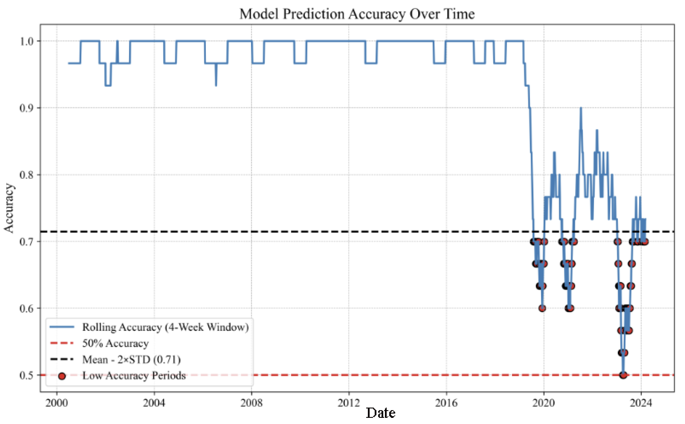
We analyze these fluctuations by examining model accuracy, taking the high-performing and high-accuracy XGBoost model as an example, as illustrated in Figure 7. The blue line represents the model accuracy calculated on a rolling 4-week basis, while the red dashed line indicates a 50% accuracy level, serving as the threshold for assessing model effectiveness. Accuracy above this line suggests that the model’s predictive performance surpasses random guessing, which is a critical minimum standard in practical applications. The black dashed line, representing the mean minus twice the standard deviation, marks the boundary for performance evaluation, identifying periods of significantly low performance. The model maintained an accuracy rate above 90% for most of the time. However, near 2020, there was a significant drop in predictive accuracy, with subsequent fluctuations and no stable periods. This period coincided with the outbreak of COVID-19, which had a profound impact on global economic activities and caused unprecedented volatility in the crude oil market. The pandemic led to a slowdown in global economic activities, mainly stalling the aviation and transportation industries, resulting in a sharp decline in oil demand. Simultaneously, OPEC+ initially disagree on production cuts, leading to an oversupply in the market. In April 2020, WTI crude oil futures prices historically fell below zero, causing market panic. From 2020 to 2024, in addition to pandemic-induced market volatility, various extreme events such as the Russo–Ukrainian War and changes in OPEC’s production decisions caused energy market fluctuations, leading to low and unstable model accuracy. This indicates a significant decline in the model’s predictive ability under extreme market conditions and economic uncertainty, reflecting inadequacies in adapting to new market dynamics caused by the pandemic and other special events.

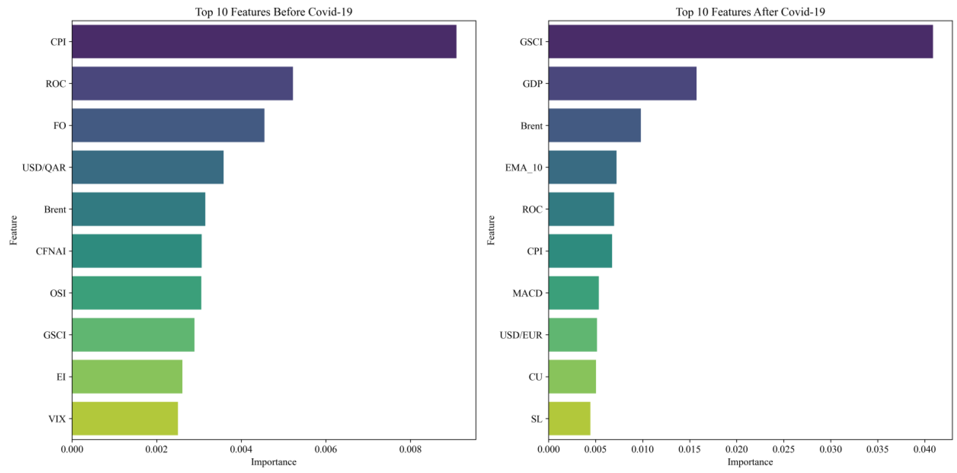
We further validated the model dynamics by examining the changes in the ranking of variable importance for predictions made by the XGBoost model before and after the pandemic, as illustrated in Figure 8. Before the pandemic, the top ten variables were dominated by the consumer price index (CPI) and other macro-economic and energy market variables, reflecting a WTI market driven by broad economic activities and energy market dynamics. After the pandemic, there was a significant shift in the landscape of feature importance. The Goldman Sachs Commodity Index (GSCI) became the most critical predictive factor, ranking several momentum indicators highly. This shift suggests that during periods of global economic turbulence, the relevance of direct commodity prices in predicting crude oil investment returns increased, and technical indicators, capable of rapidly tracking market dynamics, played a more significant role. The changes in the importance of these model variables, both before and after the pandemic, highlight the market volatility triggered by COVID-19 and underscore the dynamic shifts in key variables and fluctuations in model effectiveness during different phases of the crisis in predicting WTI returns. This demonstrates the dynamism that significant market changes may bring to machine learning models when predicting financial time series.

This shift in variable importance reflects deeper changes in market drivers under the impact of the COVID-19 pandemic. The increased prominence of GSCI and GDP after the pandemic suggests that broader commodity market trends and macroeconomic growth expectations became more significant in forecasting WTI returns, likely due to heightened global economic uncertainty and synchronized shocks across markets. The elevated importance of technical indicators, such as EMA and MACD, indicates that market participants may have relied more on short term trading signals and price momentum to guide investment decisions amid volatility and rapidly changing market conditions.

These findings underscore the dynamic and adaptive nature of financial markets in response to major global events. The observed patterns suggest that during stable periods, fundamental macroeconomic and energy-specific variables are primary drivers of crude oil returns. However, during and after periods of crisis, the market’s attention may shift more towards broad commodity indices, macroeconomic growth measures, and technical trading signals. This highlights the necessity for flexible modeling frameworks that can swiftly adapt to changing market regimes.

From a practical perspective, these results have important implications for both investors and policymakers. For investors, dynamically adjusting model features or portfolio strategies in response to shifting market drivers can enhance prediction accuracy and risk management. For policymakers, understanding which variables gain prominence during crises can help in monitoring market stability and the effectiveness of intervention policies.

5.4. Robustness Analysis

(1)

Rolling window

We tested the robustness of our models by extending the forecasting period from a 4-week rolling window to an 8-week rolling window. This approach assessed the sustainability of different models in terms of performance metrics and evaluated their adaptability over a slightly extended forecasting horizon.

As shown in

Table 8. Forecast results in 8 week rolling.

Model	MSE	${\mathit{R}}^2$	MAE	RMSE	Accuracy
OLS	0.0053	0.2487	0.0374	0.0731	0.5286
XGBoost	0.0052	0.2648	0.0151	0.0723	0.7592
Random Forest	0.0063	0.1092	0.0344	0.0796	0.5685
CNN	0.0068	0.0465	0.0401	0.0824	0.4555
BP	0.0068	0.0445	0.0389	0.0825	0.5045
MLP	0.0064	0.1065	0.0382	0.0797	0.4928
LSTM	0.0060	0.1519	0.0375	0.0777	0.5231

, after extending the rolling window, the error metrics (MSE, MAE, RMSE) slightly increased, and accuracy decreased slightly, yet the models still maintained a good performance level comparable to the 4-week rolling performance. The ranking of model performances remained unchanged, with XGBoost continuing to show the best results. Although all models displayed some sensitivity to the extended forecasting window, they still performed excellently on evaluation metrics, indicating that our machine learning models are a very robust choice for predicting WTI returns. Additionally, it was found that models with shorter rolling forecasting periods demonstrated superior effectiveness and adaptability.

(2)

Variable selection

After passing the robustness test with an adjusted rolling window, we further tested the robustness of our model predictions by modifying the variables. As shown in

Table 9. Forecast results in 4 week rolling using Top 10 variables.

Model	MSE	${\mathit{R}}^2$	MAE	RMSE	Accuracy
OLS	0.0049	0.3103	0.0336	0.0700	0.5858
XGBoost	0.0047	0.3428	0.0115	0.0684	0.7743
Random Forest	0.0050	0.2968	0.0182	0.0708	0.7397
CNN	0.0039	0.4537	0.0327	0.0624	0.6094
BP	0.0037	0.4848	0.0306	0.0606	0.6153
MLP	0.0036	0.4971	0.0304	0.0598	0.6258
LSTM	0.0050	0.2958	0.0335	0.0707	0.6102

, we selected the top 10 important variables from a combination of seven nonlinear models for prediction input and then reviewed the model’s evaluation metrics. All models demonstrated significant improvements: error metrics decreased, and accuracy levels increased. Compared to deep learning models, the OLS, XGBoost, and random forest models exhibited slight performance enhancements, underscoring their stability in scenarios with reduced features. Conversely, CNN, BP, MLP, and LSTM models, due to the characteristics of neural networks, benefited from using highly correlated input variables, which allowed for faster convergence and improved more prediction performance. However, when using all variables as inputs, the performance might decrease due to increased model complexity. Therefore, these deep learning models, being more sensitive to data disturbances, showed less robustness when adjusting input variables than OLS, XGBoost, and random forest models.

5.5. Mechanism

In forecasting WTI returns, the impact of different variable mechanisms on prediction accuracy is crucial. This section analyzes five major variable mechanisms: macroeconomic, financial and futures markets, energy markets, momentum, and natural disaster counts, evaluating their importance in the best performing XGBoost model. As shown in Figure 9, momentum variables have the most minor error indicators and the highest accuracy, demonstrating the best prediction performance among all mechanisms. This result aligns with the existing empirical evidence on momentum effects in financial markets, where recent price trends tend to persist over short horizons. In the context of oil markets, such persistence may reflect gradual information diffusion, investor herding, or technical trading, all of which can reinforce short-term price movements, given that they reflect market trends and dynamics in real time and provide immediate market sentiment and trend changes, unmatched by other financial or macroeconomic variables.

The second best-performing mechanism is the financial and futures markets, while exogenous shocks and uncertainty rank lowest. The strong predictive power of financial and futures market variables is economically intuitive, as these markets quickly aggregate and reflect participants’ heterogeneous expectations and risk assessments. Futures prices and trading volumes serve as forward looking indicators that promptly react to new information, providing timely signals for spot returns. The liquidity and transparency of these markets further enhance the quality and informativeness of the data. Financial and futures markets are closely linked to WTI prices; feature prices and trading volumes directly reflect market participants’ expectations and behavior. These variables offer timely and forward-looking information, aiding in more accurate predictions of WTI returns. Additionally, financial market data are typically more comprehensive, systematic, higher quality, and more readily available, which may also contribute to their superior predictive performance.

In the case of sustainability and external risk variables, their low importance ranking may be attributed to the fact that their effects on the crude oil market are often gradual, long-term, and diffuse, rather than immediate or directly observable. Many sustainability-related factors, such as environmental policies or shifts in global energy demand, unfold over extended periods and are slowly incorporated into market expectations and prices. As a result, their incremental predictive value for short term return forecasting tends to be limited, which reduces their relative importance within the model.

6. Conclusions

This study identifies the most suitable machine learning models for predicting WTI returns. We collected WTI price data from 1 January 2000 to 31 March 2024, calculated weekly returns, and employed various machine learning models for predictions. To enhance the accuracy of forecasts, we selected 55 variables from five different mechanisms that could influence WTI returns as model inputs. We utilized a set of evaluation metrics and conducted a 4-week rolling forecast to compare the accuracy and performance of different models.

Firstly, we compare the forecasting performance of the models with and without the inclusion of sustainability and external risk variables. The results show that the inclusion of these variables significantly improves predictive accuracy, as reflected by lower MSE, MAE, and RMSE values. This demonstrates that sustainability and external risk factors play an important role in forecasting WTI returns. In terms of model performance, XGBoost consistently delivers the best results, with error metrics noticeably lower than those of the other models. When sustainability and external risk variables are incorporated, the predictive accuracy of XGBoost further improves, surpassing the next best model by 20%.

Next, we utilized SHAP to interpret the models, linking the importance of various predictors to broader economic and market dynamics. For example, the emphasis on momentum variables (e.g., ROC) reveals that short-term price shifts play a pivotal role in shaping future returns, reflecting how investor sentiment and rapid market swings can override longer-term fundamentals in volatile periods. While linear models center largely on momentum variables, nonlinear methods unearth a wider range of influential features, suggesting that intricate interplays between macroeconomic and financial factors also impact WTI returns.

Following simulated strategy validation, we confirmed that machine learning models can yield profits for investors. XGBoost not only showcases top-tier predictive accuracy but also delivers the highest capital gains. An examination of accuracy curves shows a marked decline after the onset of COVID-19, underscoring how external shocks can destabilize even high-performing models. More critically, the most influential variable shifted from CPI to GSCI post-pandemic, highlighting how global commodity index fluctuations became more relevant than usual during crisis conditions. These dynamics present tangible lessons for developing future market resilience strategies, such as incorporating rapid-response variables (e.g., momentum or broader commodity indices) and adjusting hedging positions swiftly when faced with large-scale disruptions.

Finally, by comparing different groups of variables and evaluating their performance within the XGBoost model, we found that momentum mechanisms yielded the highest predictive accuracy, followed by variables representing financial and futures markets. This underscores the practical value of momentum indicators such as ROC for investors seeking to capture short-term market trends. In contrast, sustainability variables exhibited the lowest importance in the model. This may be attributed to the gradual and long term nature of their market impact: sustainability factors typically influence the crude oil market over extended periods and are slowly incorporated into prices. As a result, their incremental predictive value for short-term return forecasting is limited, which explains their lower ranking in variable importance.

Our findings highlight that sustainability and external risk factors are not just supplementary inputs, but essential components for effective market monitoring and energy regulation. Incorporating these variables into forecasting models enables policymakers to identify emerging risks more quickly and to design targeted interventions that can stabilize markets during periods of heightened volatility. Moreover, the use of interpretable machine learning techniques helps authorities trace the underlying causes of price fluctuations, providing a stronger evidence base for regulatory action. For sustainable development, aligning financial forecasting with ESG and climate-related indicators has practical value beyond prediction accuracy. By reflecting sustainability goals in return forecasts, investors and policymakers can better allocate capital to projects that support cleaner energy and climate adaptation. This approach promotes a more resilient energy system, one that is better equipped to handle shocks and advances the long-term transition toward lower carbon markets. As a result, integrating these variables into predictive models offers a concrete pathway to link investment decisions with the broader goals of energy security and environmental responsibility.

Overall, this research highlights the strengths of XGBoost in crude oil return prediction but also reveals important limitations. The model’s dependence on historical trends means it struggles to predict unprecedented shocks, such as those brought by the COVID-19 pandemic or geopolitical crises. The pandemic revealed shifts in model accuracy and key variables, highlighting the need for greater adaptability. The study’s focus on weekly returns, while smoothing noise, may overlook intraday dynamics critical during volatile periods. Future research should integrate high-frequency data, such as intraday prices and real-time sentiment analysis, to improve responsiveness. Expanding variables to include geopolitical indices and renewable energy trends can enhance model comprehensiveness. Hybrid models combining machine learning with regime-switching approaches could better handle extreme events. Finally, exploring cross-market interactions and longer-term predictions would deepen insights into structural market shifts, aiding both investors and policymakers in navigating evolving energy markets.