Risk-Sensitive Deep Reinforcement Learning for Portfolio Optimization

Abstract

Navigating the complexity of petroleum futures markets—marked by extreme volatility, geopolitical uncertainty, and macroeconomic shocks—demands adaptive and risk-sensitive strategies. This paper explores an Adaptive Risk-sensitive Transformer-based Deep Reinforcement Learning (ART-DRL) framework to improve portfolio optimization in commodity futures trading. While deep reinforcement learning (DRL) has been applied in equities and forex, its use in commodities remains underexplored. We evaluate DRL models, including Deep Q-Networks (DQN), Proximal Policy Optimization (PPO), Advantage Actor-Critic (A2C), and Deep Deterministic Policy Gradient (DDPG), integrating dynamic reward functions and asset-specific optimization. Empirical results show improvements in risk-adjusted performance, with an annualized return of 1.353, a Sharpe Ratio of 4.340, and a Sortino Ratio of 57.766. Although the return is below DQN (1.476), the proposed model achieves better stability and risk control. Notably, the models demonstrate resilience by learning from historical periods of extreme volatility, including the COVID-19 pandemic (2020–2021) and geopolitical shocks such as the Russia–Ukraine conflict (2022), despite testing commencing in January 2023. This research offers a practical, data-driven framework for risk-sensitive decision-making in commodities, showing how machine learning can support portfolio management under volatile market conditions.

1. Introduction: The Challenge of Risk in Commodity Markets

Commodity futures markets are characterized by volatility driven by macroeconomic cycles, geopolitical tensions, and supply disruptions. Traditional portfolio methods, such as mean-variance optimization, often assume stable correlations and normal return distributions. These assumptions tend to break down in highly volatile environments, exposing investors to sudden drawdowns and unpredictable risks (Bahoo et al., 2024). Recent research also highlights the importance of tailoring portfolio strategies to region-specific risks and exposures, as seen in ETF-focused studies such as (Jaffri et al., 2025), which demonstrate how alternative modeling approaches can provide risk-adjusted performance insights under market uncertainty.

This study proposes an adaptive framework: Adaptive Risk-sensitive Transformer-based Deep Reinforcement Learning (ART-DRL) to address these challenges. Unlike static models, DRL can adjust continuously to changing market conditions. We explore several DRL agents: Deep Q-Networks (DQN) for discrete decisions, Proximal Policy Optimization (PPO) for stable policy updates, Deep Deterministic Policy Gradient (DDPG) for continuous actions, and Advantage Actor-Critic (A2C) for combining value and policy learning (Chen et al., 2021; Koratamaddi et al., 2021; Shakya et al., 2023). The ART-DRL framework dynamically selects the most suitable agent as market conditions evolve.

Commodity futures differ significantly from equities, forex, and even financial futures in terms of market structure, underlying drivers, and risk characteristics. Unlike equities and forex, which are primarily driven by macroeconomic indicators, interest rates, and investor sentiment, commodity futures are also subject to physical supply–demand imbalances, seasonal production cycles, storage constraints, and weather shocks (Bahoo et al., 2024). For example, agricultural and energy markets often experience spikes in volatility due to geopolitical disruptions, OPEC announcements, or climate-related supply risks. These idiosyncratic factors introduce abrupt price movements and nonlinear risk patterns, making traditional assumptions such as normal returns and stable correlations less reliable (Bahoo et al., 2024; Shakya et al., 2023).

In addition, compared to other categories of futures, such as interest rate or equity index futures, commodity futures are more prone to expiration effects, basis risk, and delivery constraints, which can complicate modeling and trading strategies. These structural complexities require more adaptive and risk-sensitive approaches. Therefore, the challenges discussed in this paper are both relative to other futures markets and particularly pronounced compared to equities and the foreign exchange (forex) markets. To address the unique challenges of commodity futures markets, we evaluated three deep reinforcement learning (DRL) strategies. Method 1 uses a single DRL agent (DQN, PPO, A2C, or DDPG) to learn static trading policies. Method 2 utilizes multiple agents that run independently to capture diverse market patterns. Method 3 introduces our proposed Adaptive Risk-sensitive Transformer-based DRL (ART-DRL) framework, which dynamically switches between agents based on rolling performance. Through a comparative analysis of these three approaches, we demonstrate that ART-DRL delivers superior risk-adjusted performance, particularly under volatile market conditions.

This study demonstrates the robustness of our model in navigating volatile market conditions, which are quantitatively defined as periods when the rolling standard deviation of daily returns exceeds the long-term historical average by more than one standard deviation. This objective, data-driven criterion enables systematic identification of phases characterized by elevated uncertainty and stress within the petroleum futures market.

Volatility presents a persistent challenge in commodity futures trading, where effective risk management and performance optimization are essential. To address this, we propose the ART-DRL framework, designed to enhance returns while maintaining robustness across diverse market conditions. This is particularly relevant given recent market disruptions, such as post-COVID volatility and the geopolitical energy shocks observed during 2023–2024.

We evaluate ART-DRL against two baseline approaches: (i) a single DRL agent applied across all conditions, and (ii) multiple independent DRL agents without coordination. In contrast, ART-DRL incorporates an adaptive switching mechanism that dynamically selects strategies based on real-time performance metrics.

Volatile market periods are quantitatively defined as intervals in which the rolling standard deviation of daily returns exceeds the long-term historical average by more than one standard deviation, capturing episodes of increased uncertainty and market stress.

By integrating risk-sensitive performance metrics and a dynamic strategy-switching mechanism, our approach delivers actionable insights for institutional investors and risk-aware traders. For comparative evaluation, we benchmark the performance of our framework against a conventional buy-and-hold strategy. To address risk in highly volatile petroleum futures markets, our model incorporates both volatility-sensitive input features and risk-adjusted evaluation metrics. The risk sensitivity of each approach is detailed in Section 4.3.

2. Advances in Deep Reinforcement Learning for Financial Applications

2.1. DRL in Algorithmic Trading

Recent research has significantly expanded the application of deep reinforcement learning (DRL) in financial markets through innovative architectures and data integration (Hambly et al., 2023):

2.1.1. Multimodal Data Integration

• (Jiajie & Liu, 2025) proposed an innovative multimodal deep reinforcement learning framework, offering significant advances in portfolio optimization by effectively integrating diverse data modalities.
• (Nan et al., 2020) introduced the DRL enhanced by sentiment by combining price data with news sentiment, improving trading decisions.
• (Koratamaddi et al., 2021) and (Fu et al., 2025) demonstrated that the incorporation of alternative data, specifically the sentiment of the news, macro-indicators, and macro-events, can significantly improve the performance of the DRL model.

2.1.2. Architectural Innovations

• (Yang et al., 2020) proposed an ensemble DRL architecture designed to deliver robust performance across different market regimes.
• (Zhang et al., 2020) integrated Q learning with LSTM networks to allow strategy adaptation in both equity and futures markets.

2.2. Specialized Trading Domains

• High-Frequency Trading: (Ganesh & Rakheja, 2018) achieved superior execution quality in low-latency environments using DRL, outperforming traditional rule-based systems by 18%.
• Risk Management: (Bao et al., 2019) developed a multi-agent DRL system to optimize liquidation strategies under price impact and inventory constraints, reducing slippage by 22%.
• Derivatives Hedging: (Buehler et al., 2019) introduced a DRL-based deep hedging framework, demonstrating a 30% reduction in residual risk compared to conventional delta hedging in nonlinear markets.

2.3. Commodity Futures Trading

Recent studies have increasingly demonstrated the potential of deep reinforcement learning (DRL) in commodity futures markets:

• (Du et al., 2023) applied variational mode decomposition to Brent crude oil futures, integrating the decomposed features into an ensemble DRL framework. While effective in capturing non-stationary components, their model lacked adaptive agent switching mechanisms to dynamically adjust to changing market conditions.
• (Massahi & Mahootchi, 2024) developed a GRU-enhanced Deep Q-Network (DQN) model to address futures contract execution challenges. Although their approach improved intra-contract trading, it was primarily limited to managing single-contract positions and did not extend to portfolio-level optimization across multiple futures instruments.

In contrast, much of the earlier literature has focused on the application of DRL to equity and foreign exchange (FX) markets. For instance, (Moody & Saffell, 2001) introduced a recurrent reinforcement learning approach for stock trading, demonstrating its potential to model temporal dependencies in equity markets. Similarly, (Deng et al., 2016) explored deep learning architectures for financial signal representation and trading, providing a foundation for applying neural networks to complex financial time series forecasting problems.

While these prior works have advanced DRL applications across different financial instruments, the unique characteristics of commodity futures—including non-stationary price behavior, seasonality, and abrupt regime shifts—pose additional challenges that require models capable of learning long-range temporal dependencies. This motivates the incorporation of Transformer-based architectures, which have demonstrated superior performance in sequence modeling tasks across various domains.

2.4. Methodological Foundations

The Transformer architecture, first introduced by (Vaswani et al., 2017), has revolutionized sequence modeling through its self-attention mechanism, enabling the efficient extraction of long-range temporal dependencies without reliance on recurrent structures. When combined with DRL, Transformers offer a powerful framework for learning intricate temporal patterns inherent in financial markets, particularly under conditions of structural volatility and regime shifts.

The primary deep reinforcement learning algorithms utilized in this study are:

• Deep Q-Network (DQN) (Mnih, 2013): Uses Q-learning with deep networks, stabilized by experience replay and target networks.
• Advantage Actor-Critic (A2C) (Mnih et al., 2016): Combines policy and value learning, improving sample efficiency.
• Deep Deterministic Policy Gradient (DDPG) (Lillicrap et al., 2015): Extends Q-learning to continuous action spaces using an actor-critic framework.
• Proximal Policy Optimization (PPO) (Schulman et al., 2017): Refines policy gradient methods with clipped objectives, balancing exploration and exploitation.

2.4.1. Transformer

The Transformer, introduced by (Vaswani et al., 2017), is a deep learning architecture designed for sequence modeling. Its core component, self-attention, dynamically weights input elements, capturing long-range dependencies with parallel computation. Originally developed for natural language processing, it has been successfully applied to DRL tasks, including financial market forecasting.

The Transformer architecture features an encoder–decoder structure. The encoder transforms inputs into contextual representations, while the decoder generates outputs from these embeddings. Each layer within the encoder and decoder comprises:

• Multi-Head Self-Attention: Computes dependencies between input elements in parallel.
• Feedforward Network (FFN): Applies nonlinear transformations for feature extraction.
• Residual Connections and Layer Normalization: Improve gradient flow and model stability.
• Positional Encoding: Encodes sequential order since self-attention lacks inherent positional awareness.

Self-Attention Mechanism

Self-attention models pairwise token dependencies via learnable projections:

$$\mathrm{Q}=\mathrm{X}{\mathrm{W}}^{\mathrm{Q}},\mathrm{K}=\mathrm{X}{\mathrm{W}}^{\mathrm{K}},\mathrm{V}=\mathrm{X}{\mathrm{W}}^{\mathrm{V}},$$

where $\mathrm{Q}$, $\mathrm{K}$, and $\mathrm{V}$ are the query, key, and value matrices, respectively. The attention output is

$$Attention\left(\mathrm{Q},\mathrm{K},\mathrm{V}\right)=Softmax\left({\displaystyle \frac{\mathrm{Q}{\mathrm{K}}^{\mathrm{T}}}{\sqrt{{\mathrm{d}}_k}}}\right)\mathrm{V}.$$

Multi-Head Attention

To capture information from multiple representation subspaces, h self-attention heads run in parallel:

$$MultiHead\left(\mathrm{Q},\mathrm{K},\mathrm{V}\right)=\mathrm{Concat}\left({\mathrm{Z}}_1,{\mathrm{Z}}_2,\dots ,{\mathrm{Z}}_h\right){\mathrm{W}}^{\mathrm{O}},$$

where ${\mathrm{Z}}_i$ is the output of the i-th head.

Feed-Forward Network

Each Transformer layer includes a position-wise feed-forward network (FFN):

$$\mathrm{FFN}\left(\mathrm{x}\right)=ReLU\left({\mathrm{W}}_1\mathrm{x}+{\mathrm{b}}_1\right){\mathrm{W}}_2+{\mathrm{b}}_2,$$

adding non-linearity and enhancing feature representation.

Positional Encoding

Because self-attention is order-agnostic, sinusoidal positional encodings are added:

$$\mathrm{PE}\left(\mathrm{pos},i\right)=\left\{\begin{array}{cc}sin\left(\mathrm{pos}{\omega }_k\right),\hfill & \mathrm{if}i=2k,\hfill \\ cos\left(\mathrm{pos}{\omega }_k\right),\hfill & \mathrm{if}i=2k+1,\hfill \end{array}\right.{\omega }_k={\displaystyle \frac{1}{10,{000}^{\frac{2k}{d}}}},$$

where ${\omega }_k$ ensures unique encoding for each position.

2.4.2. Markov Decision Process (MDP)

Trading is modeled as a Markov Decision Process (MDP), which is defined by the following components:

• State Space (S): Represents the market conditions at each time step.
• Action Space (A): Defines the possible adjustments to the portfolio.
• Transition Probability (P): Determines how the State evolves based on a given action.
• Reward Function (R): Quantifies performance based on returns.
• Discount Factor ($\gamma$): Controls the trade-off between short-term and long-term rewards.

The objective is to learn an optimal policy $\pi$ that maximizes the expected cumulative rewards.

2.4.3. Deep Reinforcement Learning Models

This section outlines the training agents used in this study.

Deep Q-Network (DQN)

DQN (Mnih, 2013) enhances traditional Q-learning by incorporating deep neural networks to approximate the Q-value function. It stabilizes the training process using the following techniques:

• Experience Replay: This method involves storing past experiences to enable batch training, thereby improving learning efficiency.
• Target Network: A separate Q-network is maintained to decrease volatility during training.

DQN aims to optimize the Q-function by minimizing the following loss function:

$$L=\mathrm{E}\left[{\left(\mathrm{r}+\gamma \underset{a^{\prime }}{max}\mathrm{Q}(s^{\prime },a^{\prime })-\mathrm{Q}(s,a)\right)}^2\right]$$

Advantage Actor-Critic (A2C)

A2C (Mnih et al., 2016) combines policy-based and value-based methods. It consists of the following:

• Actor: Learns the policy $\pi (a\mid s)$.
• Critic: Estimates the state value function $V\left(s\right)$.

The advantage function improves stability:

$$A(s,a)=\mathrm{Q}(s,a)-\mathrm{V}\left(s\right)$$

Policy updates follow:

$$L_a=-log\left(\pi (a\mid s)\right)A(s,a)$$

Deep Deterministic Policy Gradient (DDPG)

DDPG (Lillicrap et al., 2015) extends DQN to continuous action spaces using an actor-critic framework:

• Actor: Outputs a deterministic action $\mu \left(s\right)$.
• Critic: Estimates $Q(s,a)$.

It stabilizes learning using target networks and experience replay. The critic is updated by minimizing the following:

$$L=\mathrm{E}\left[{\left(\mathrm{r}+\gamma {\mathrm{Q}}^{\prime }\left(s^{\prime },{\mu }^{\prime }\left(s^{\prime }\right)\right)-\mathrm{Q}(s,a)\right)}^2\right]$$

Proximal Policy Optimization (PPO)

PPO (Schulman et al., 2017) refines policy gradient methods using a clipped objective function:

$$L_{\mathrm{CLIP}}\left(\theta \right)={\mathrm{E}}_t\left[min\left(r_t\left(\theta \right)A^t,\mathrm{clip}\left(r_t\left(\theta \right),1-ϵ,1+ϵ\right)A^t\right)\right]$$

where $r_t\left(\theta \right)$ is the probability ratio between the new and old policy. Clipping ensures stable updates.

PPO is widely used due to its simplicity, efficiency, and robust performance in high-dimensional tasks.

2.5. Our Contributions Advance These Works Through

• ART-DRL: Adaptive Risk-sensitive Transformer-based DRL (ART-DRL) framework, a novel adaptive agent-switching mechanism based on real-time performance.
• Diversified Portfolio Application: Covers Brent crude oil, RBOB spreads, and Gasoil crack spreads.
• Risk-Aware Design: Incorporates drawdown-optimized reward functions and evaluates performance using the Sharpe, Sortino, and Calmar ratios.
• Transformer Integration: Enables temporal and cross-asset feature extraction for improved decision-making.

3. Data Preparation

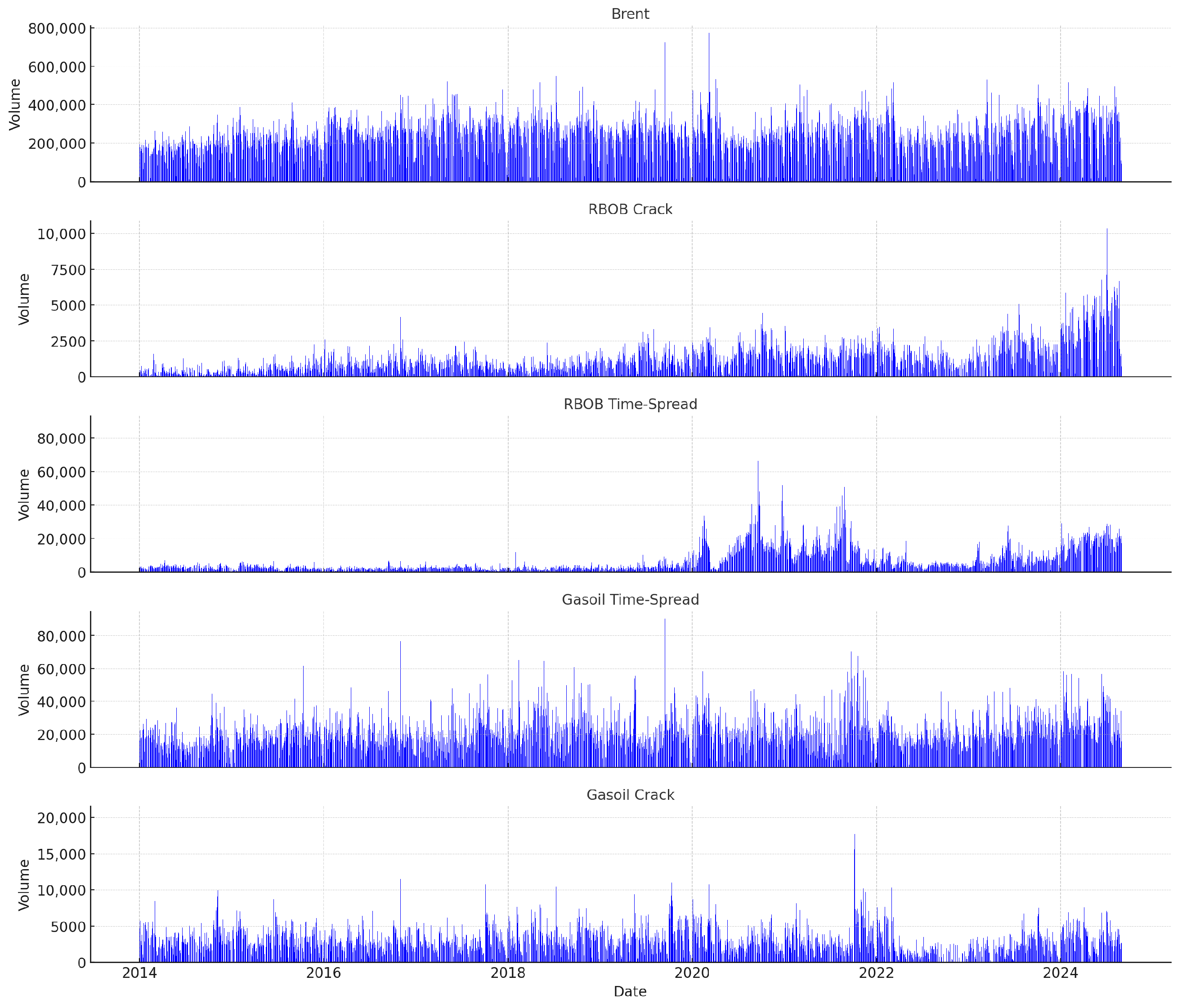
We employ historical daily price and volume data for petroleum futures contracts sourced from the Intercontinental Exchange (ICE) and the New York Mercantile Exchange (NYMEX), covering the period from January 2014 to January 2024. This decade encompasses significant structural shifts in global oil markets.

The analysis focuses on actively traded contracts representing key benchmarks for U.S. and European energy commodities. The selected instruments include:

• Brent Crude Oil Futures (ICE: B)—a global benchmark for European crude oil pricing;
• RBOB Crack Spread (NYMEX)—the margin between U.S. gasoline (RBOB) and Brent crude, representing refining economics;
• RBOB Time Spread (NYMEX)—the price differential between near-term and forward-month RBOB contracts;
• Gasoil Crack Spread (ICE)—the margin between gasoil and Brent crude oil, used as a proxy for European distillate profitability;
• Gasoil Time Spread (ICE)—the price difference between successive delivery months for gasoil contracts.

To construct continuous price series across contract expirations, we apply an open interest-weighted rolling strategy. For each asset, the front-month contract is rolled to the next based on open interest, typically on the last trading day of the current contract’s active month. Back-adjustment is performed using the price differential at the rollover point to eliminate discontinuities and preserve return consistency.

The dataset includes Open, High, Low, and Close (OHLC) prices as well as trading volumes. Volume serves dual purposes: (i) as a liquidity filter to exclude thinly traded instruments, and (ii) as a dynamic input feature to inform agent learning behavior.

In addition to raw price and volume data, we derive several technical indicators widely used in quantitative trading and financial modeling:

• Moving Average (MA)—smoothing of past prices over a fixed window to identify trend direction;
• Relative Strength Index (RSI)—a momentum oscillator that signals overbought or oversold conditions;
• Moving Average Convergence Divergence (MACD)—a trend-following indicator based on the convergence and divergence of two moving averages;
• Bollinger Bands—volatility bands around a moving average to capture price dispersion;
• Volatility Metrics—including rolling standard deviation and exponentially weighted volatility to quantify market uncertainty.

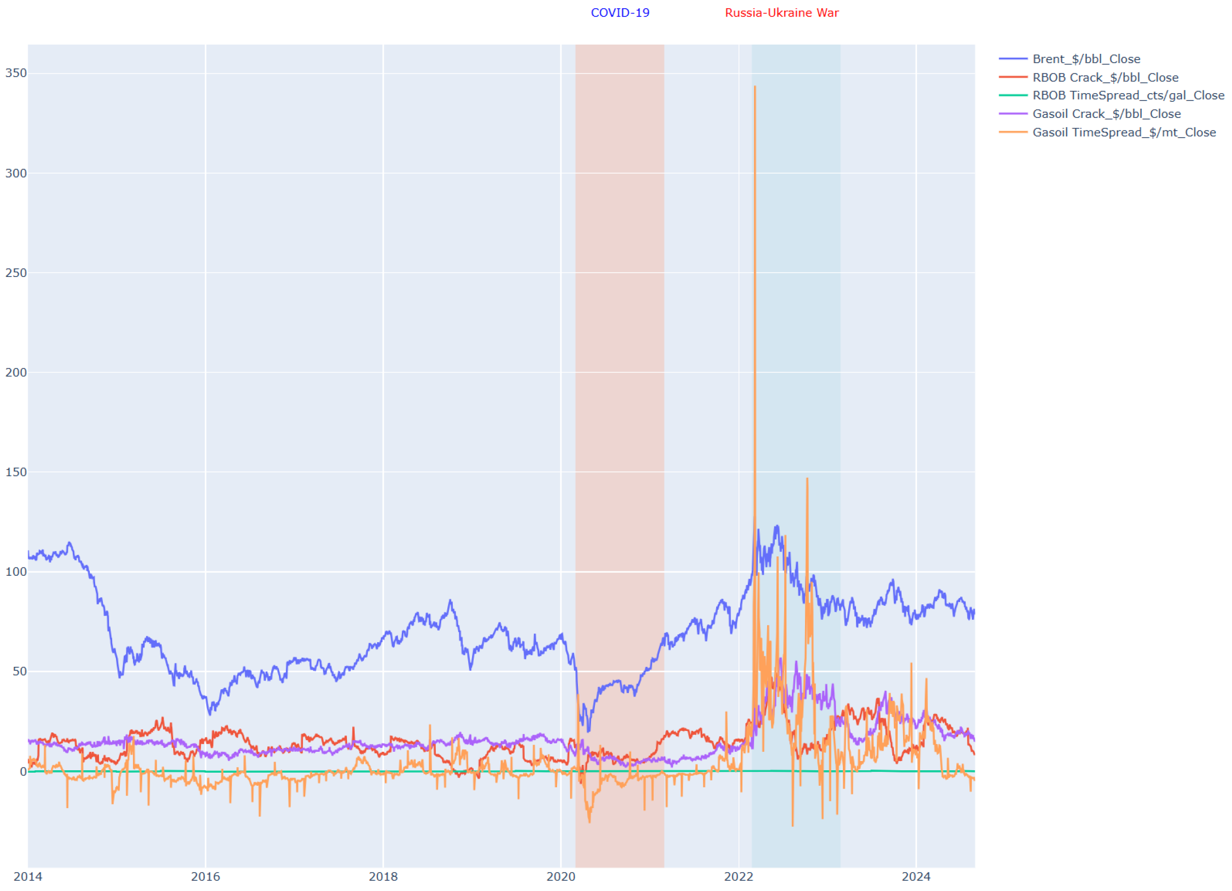
Figure 1 and Figure 2 illustrate key characteristics of the dataset. Figure 1 presents the daily trading volumes for the selected contracts, while Figure 2 shows the corresponding continuous futures price series over the 10-year horizon.

Technical Indicators

In addition to the fundamental data provided by the exchange, technical indicators are generated as features to enhance model training:

• Simple Moving Average (SMA) smooths out price data over a specified time, offering a clearer picture of trends by reducing “noise.”

  $${\mathrm{SMA}}_n={\displaystyle \frac{{\sum }_{i=1}^n{\mathrm{ClosePrice}}_i}{n}}$$
  The current study uses periods of 50 days and 200 days. Longer SMAs (such as the 200-period) help indicate the overall trend, while shorter SMAs (like the 50-period) provide recent trend direction, enabling the model to distinguish between long-term and short-term trends.
• Exponential Moving Average (EMA) is a weighted average of recent closing prices, giving more weight to recent prices to react faster to changes than SMA.

  $${\mathrm{EMA}}_n=\alpha \times \mathrm{Close}+(1-\alpha )\times {\mathrm{EMA}}_{n-1},\alpha ={\displaystyle \frac{2}{n+1}}$$
  The current study uses periods of 50 days and 200 days. EMA is responsive to recent price changes, helping the model capture quicker shifts in trends compared to SMA.
• Relative Strength Index (RSI) measures the magnitude of recent price changes to assess overbought or oversold conditions.

  $$\mathrm{RSI}=100-{\displaystyle \frac{100}{1+\frac{\mathrm{AverageGain}}{\mathrm{AverageLoss}}}}$$
  The current study uses 14 days. It helps the model identify momentum conditions that indicate potential trend reversals, thereby improving its responsiveness to changes in price direction.
• Moving Average Convergence Divergence (MACD) is the difference between a short-term and long-term EMA, often used to spot trend reversals.

  $$\mathrm{MACD}={\mathrm{EMA}}_{\mathrm{fast}}-{\mathrm{EMA}}_{\mathrm{slow}}$$

  $$\mathrm{Signal}=\mathrm{EMA}\left(\mathrm{MACD}\right)$$
  The current study uses Fast EMA (12 days), Slow EMA (26 days), and Signal Line (9 days). The MACD and its signal line help identify changes in the strength, direction, momentum, and duration of a trend.
• Average True Range (ATR) measures market volatility by calculating the average range of price over a specified period.

  $$\mathrm{TR}=max\left(\mathrm{High}-\mathrm{Low},|\mathrm{High}-\mathrm{PreviousClose}|,|\mathrm{Low}-\mathrm{PreviousClose}|\right)$$

  $${\mathrm{ATR}}_n=\mathrm{SMA}\left(\mathrm{TR}\right)$$
  The current study uses 14 days. ATR captures market volatility, allowing the model to gauge the risk and potential reward of a trade.
• Bollinger Bands consist of a moving average with two standard deviation lines, capturing price volatility.

  $$\mathrm{MiddleBand}={\mathrm{SMA}}_{20}$$

  $$\mathrm{UpperBand}=\mathrm{MiddleBand}+2\times \mathrm{StdPrice}$$

  $$\mathrm{LowerBand}=\mathrm{MiddleBand}-2\times \mathrm{StdPrice}$$
  The current study uses 20 days. It helps assess volatility and potential reversal points when prices hit the bands.
• Ichimoku Cloud is a complex indicator offering multiple support/resistance levels and trend signals. The components to form an Ichimoku cloud include:

  $$\mathrm{TenkanSen}={\displaystyle \frac{{\mathrm{High}}_9+{\mathrm{Low}}_9}{2}}$$

  $$\mathrm{KijunSen}={\displaystyle \frac{{\mathrm{High}}_{26}+{\mathrm{Low}}_{26}}{2}}$$

  $$\mathrm{SenkouSpanA}={\displaystyle \frac{\mathrm{TenkanSen}+\mathrm{KijunSen}}{2}}$$

  $$\mathrm{SenkouSpanB}={\displaystyle \frac{{\mathrm{High}}_{52}+{\mathrm{Low}}_{52}}{2}}$$

  $$\mathrm{ChikouSpan}={\mathrm{Close}}_{t-26}$$
  The Ichimoku Cloud offers a comprehensive view of support, resistance, and momentum, allowing the model to identify potential reversal and continuation patterns.

4. Methodology

We designed and tested an adaptive deep reinforcement learning (DRL) framework to optimize portfolios in the petroleum futures market.

Implementation Details: All experiments were implemented in Python 3.9 (Python Software Foundation, Wilmington, DE, USA) using the PyTorch 1.13.1 deep-learning framework. Training and evaluation were performed on a workstation equipped with a GeForce RTX 3090 GPU (NVIDIA Corporation, Santa Clara, CA, USA), an Intel Core i9-12900K CPU (Intel Corporation, Santa Clara, CA, USA), and 64 GB DDR4 RAM (Corsair Memory, Inc., Fremont, CA, USA). Although the hardware setup did not influence the model architecture or relative performance comparison, it facilitated efficient execution and accelerated the deep reinforcement learning training process.

4.1. Method 1—Single DRL Agent

This method builds a trading environment using one DRL agent at a time (DQN, PPO, A2C, DDPG). We defined the environment as a Markov Decision Process (MDP), including the State, action, reward function, and discount factor.

Portfolio Construction

The portfolio management task is formulated as a Markov Decision Process (MDP), represented by the tuple $(S,A,P,R,\gamma )$:

• State (S): The State $s_t$ at each time step comprises market information and portfolio weights across five assets (Brent crude oil, RBOB gasoline crack spread, RBOB time spread, gasoil crack spread, and gasoil time spread), represented by a 64-dimensional feature vector. A Transformer-based network processes this vector, capturing both temporal dependencies and inter-asset relationships, which are essential for portfolio rebalancing decisions (Parisotto & Salakhutdinov, 2020).
• Action (A): Actions are continuous portfolio weights that the agent allocates to each asset, constrained between 0 and 1 to ensure diversification and the sum of the weight of five assets is 1. The allocation for each asset at time t, $a_t$, is updated based on the chosen policy, which varies across the DQN, A2C, DDPG, and PPO algorithms.
• Transition (P): The transition function $P(s_{t+1}\mid s_t,a_t)$ defines the probability of moving from the current state $s_t$ to the next state $s_{t+1}$ given action $a_t$. In this study, transitions are not modeled explicitly; rather, they are driven by historical market data, allowing the environment to evolve in a data-driven manner without assuming a known stochastic process (Abuqaddom et al., 2021; Mousavi et al., 2024).
• Reward (R): The reward $r_t$ is designed to balance return and risk by incorporating both portfolio returns and volatility.
  The portfolio return at time t, denoted as $R_t$, is calculated as the weighted sum of individual asset returns:

  $$R_t=\sum _{i=1}^N{w}_{i,t-1}·{\displaystyle \frac{P_{i,t}-P_{i,t-1}}{P_{i,t-1}}}$$

  where $w_{i,t-1}$ is the weight allocated to asset i at time $t-1$, and $P_{i,t}$ is the price of asset i at time t. This formulation captures the daily change in the portfolio value driven by asset-level price movements and weight allocation.
  The reward function is defined as:

  $$r_t=log(1+R_t)+\alpha ·\mathrm{Calmar}\mathrm{Ratio}-\beta ·{\sigma }_t$$

  where the first term is the **logarithmic utility** of return, reflecting the agent’s preference for proportional growth and penalizing large negative returns.
  The Calmar Ratio at time t is computed as:

  $$\mathrm{Calmar}\mathrm{Ratio}={\displaystyle \frac{log(1+R_t)}{\mathrm{Max}\mathrm{Drawdown}+ϵ}}$$

  where the numerator reflects the log utility of return (same as the first reward term), and the denominator is the maximum drawdown encountered up to time t, regularized by a small $ϵ$ to avoid division by zero. This ratio penalizes strategies that generate returns at the cost of large drawdowns.
  The standard deviation ${\sigma }_t$ is computed using the rolling volatility of asset returns, and the constants $\alpha =0.13$ and $\beta =0.0089$, which were selected through empirical tuning based on training stability and out-of-sample risk-adjusted performance, adjust the trade-off between reward maximization and risk control.
• Discount Factor ($\gamma$): A discount factor of $\gamma =0.99$ ensures that future rewards are valued but slightly discounted, aligning the agent’s strategy with long-term reward maximization.

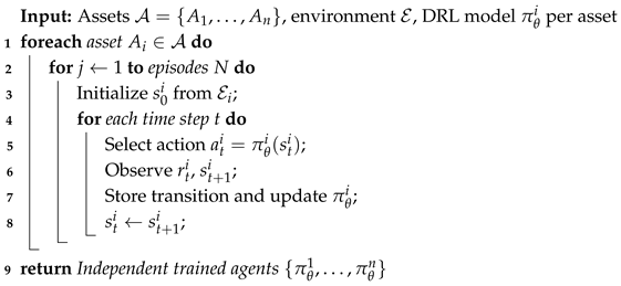
The overall training and execution pipeline for the single DRL agent used in Method 1 is detailed in Algorithm 1. This approach treats the portfolio as a single environment and learns a unified policy across all assets.

Algorithm 1: Single DRL Agent Training and Execution

4.2. Method 2—Independent DRL Agents

This method extends the design by running multiple DRL agents independently, using structured state representations and discrete action spaces to improve adaptability and performance.

4.2.1. Portfolio Construction

Portfolio management is formulated as a Markov Decision Process (MDP) with key components:

• State (S): Represents market dynamics, integrating historical data and past actions.

  –

  Historical Market Data: A $5\times 30$ matrix of technical indicators over five days. It captures trends, reversals, and momentum.

  –

  Previous Actions: The last action, ranging from $-1$ (full short) to 1 (full long), with 201 discrete positions (increments of 0.01).

  A Transformer module processes these data to extract:

  –

  Temporal Dependencies: Identifies trends in past indicators.

  –

  Inter-Asset Relationships: Captures interactions between different assets.

• Action (A): A discrete space of 201 positions in $[-1,1]$.

  –

  $-1$ (full short), 0 (neutral), 1 (full long).

  –

  Intermediate values (e.g., $-0.5$, $0.5$) represent partial exposure.

  –

  High-volatility instruments (e.g., RBOB_TimeSpread) are scaled by 100.

  –

  Positions are opened at the day’s start and closed the next day.

• Transition (T): Market state transitions as:

  $$S_{t+1}=f(S_t,A_t,M_{t+1})$$
  A Transformer network captures long-term dependencies and implicit market patterns. The episode ends if the portfolio balance reaches zero or a predefined date has passed.
• Reward (R): Defined as the log utility difference:

  $${\mathrm{reward}}_t=ln({\mathrm{balance}}_t+1)-ln({\mathrm{balance}}_{t-1}+1)$$
  The following steps define PnL and balance updates:
  • Daily PnL:

    $$\mathrm{PnL}=\mathrm{position}\mathrm{size}\times \Delta P\times \mathrm{contract}\mathrm{size}-\mathrm{fee}$$

    where:

    –

    $\Delta P=P_{\mathrm{close}}-P_{\mathrm{open}}$ (price change).

    –

    $\mathrm{fee}=\left|\mathrm{pos}\right|\times P_{\mathrm{open}}\times \mathrm{size}\times 0.0001$.

  • Balance Update:

    $${\mathrm{balance}}_t={\mathrm{balance}}_{t-1}+{\mathrm{PnL}}_t.$$
  • Reward Stabilization: Log transformation reduces extreme fluctuations. Each asset starts with a USD 10M balance.
• Discount Factor ($\gamma$): Set to $0.01$ to prioritize short-term rewards for market adaptability.

4.2.2. Asset Weight Calculation

Portfolio weights are computed as follows:

$$w_i=\left\{\begin{array}{cc}\mathrm{Round}(tanh(10·\mathrm{q}\_\mathrm{value}),2),\hfill & \mathrm{DQN}\hfill \\ \mathrm{Round}(-1+0.01·\mathrm{a},r),\hfill & \mathrm{A}2\mathrm{C}/\mathrm{PPO}\hfill \\ \mathrm{Round}(\mathrm{a},r),\hfill & \mathrm{DDPG}\hfill \end{array}\right.$$

where a represents the selected action index, portfolio weights are normalized to maintain capital constraints:

$$W_i={\displaystyle \frac{w_i}{{\sum }_{i=1}^N\left|w_i\right|}}$$

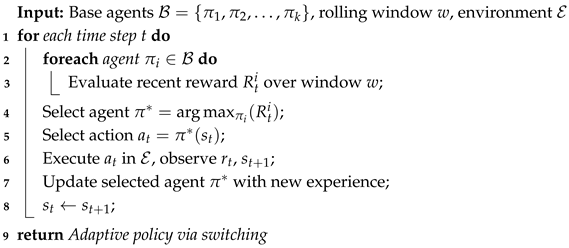
As illustrated in Algorithm 2, Method 2 trains independent DRL agents for each asset. This design allows each agent to specialize, but it lacks coordination across the portfolio.

Algorithm 2: Independent DRL Agents for Each Asset

4.3. Method 3—Adaptive DRL Strategy Switching

This method introduces an adaptive framework (ART-DRL) that dynamically switches between agents based on the 5-day rolling average PnL to optimize returns under varying market conditions.

4.3.1. Portfolio Construction

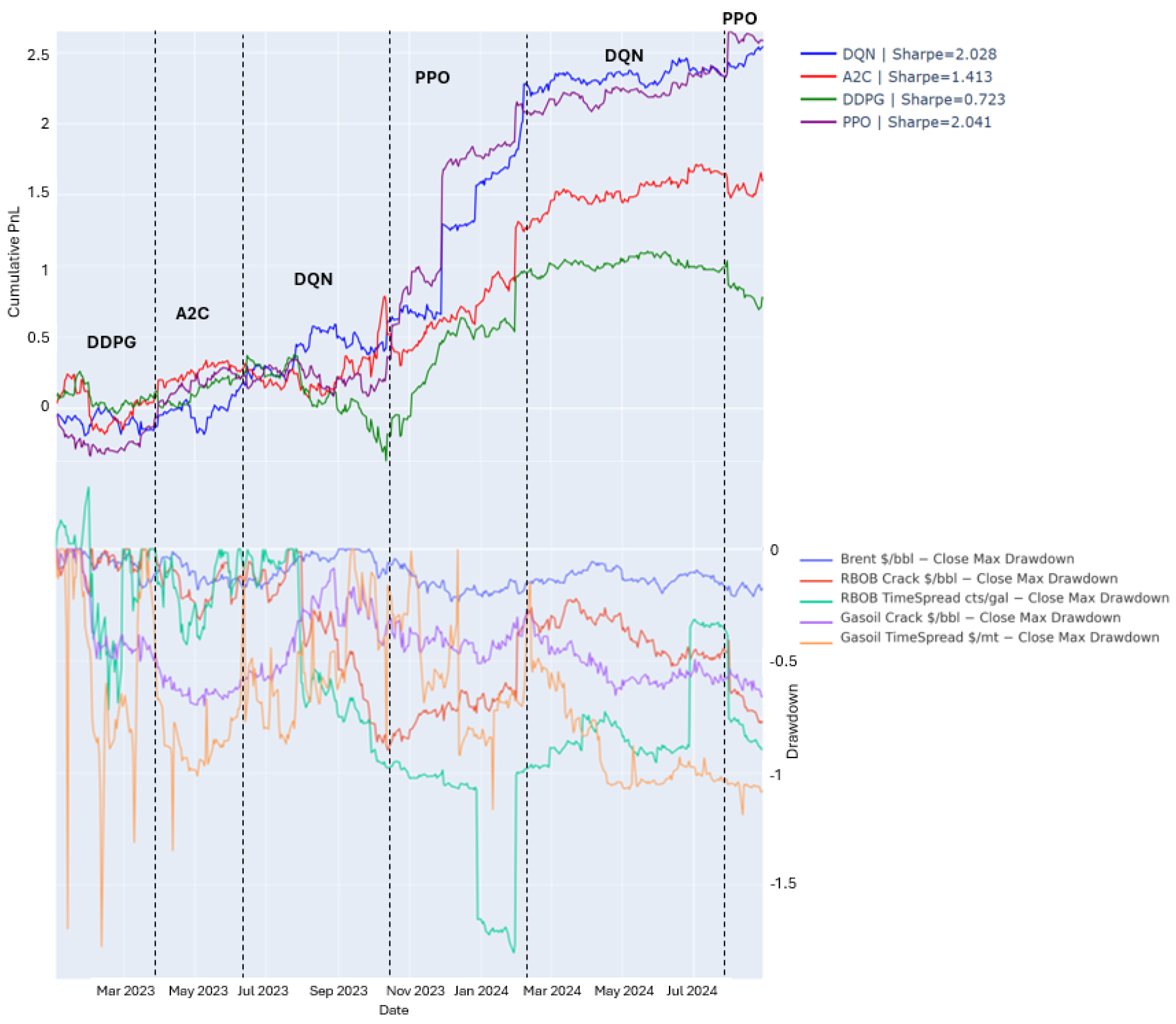
Figure 3 presents the performance of each DRL agent across distinct market phases during the test period. The x-axis denotes trading days. In the top panel, the y-axis shows cumulative P&L returns, while the bottom panel illustrates the corresponding maximum drawdowns, providing insight into both profitability and risk exposure over time.

• DDPG: Performs well in high-volatility, low-data environments due to its off-policy learning. However, it struggles as market complexity increases.
• A2C: Adapts quickly in evolving markets but lacks stability in highly complex scenarios.
• DQN: Excels during periods of high volatility (e.g., July–Nov 2023, Feb–July 2024). Its off-policy learning effectively manages risk and reduces drawdowns.
• PPO: Demonstrates steady performance in trending markets with lower volatility. It is the preferred agent from November 2023 to February 2024 and after August 2024.

The proposed Adaptive Risk-sensitive Transformer-based DRL (ART-DRL) model is a dynamic strategy that continuously switches between agents based on real-time performance. Instead of relying on a single model ART-DRL monitors the rolling 5-day cumulative PnL of all candidate agents and dynamically selects the best-performing one at each time step. It allows the framework to adjust strategies on the fly as market conditions evolve, making it more resilient across regimes compared to static approaches.

Algorithm 3 presents the ART-DRL strategy switching mechanism. It dynamically selects the best-performing agent based on a rolling performance window, enabling adaptive decision-making across market regimes.

Algorithm 3: Adaptive DRL Strategy Switching (ART-DRL)

4.3.2. Risk Sensitivity in DRL Models

In this study, risk sensitivity is integrated into the DRL framework through two primary mechanisms. First, we incorporate engineered volatility indicators into the state representation of each agent. These include the rolling standard deviation, exponentially weighted volatility, and Bollinger Band width, all of which capture different aspects of market uncertainty. These features enable the agents to adapt their behavior under varying volatility regimes.

Second, risk sensitivity is reflected in the evaluation metrics used for model comparison—namely, the Sharpe, Sortino, and Calmar ratios—which explicitly penalize models with higher variance or larger drawdowns. In the case of the ART-DRL model, the dynamic agent-switching mechanism uses these risk-adjusted metrics to guide real-time agent selection. By doing so, the model prefers strategies that offer more stable and resilient performance under uncertain conditions.

This dual incorporation of volatility-aware features and risk-adjusted evaluation criteria ensures that the proposed framework not only seeks high returns but does so while managing downside risk.

4.4. Evaluation Metrics

After training and testing, models were evaluated based on return, risk, and overall portfolio performance.

• Cumulative Return: Measures total portfolio growth over time. Defined as:

  $$R_c=\left(\prod _{t=1}^T(1+R_t)\right)-1$$

  where $R_t$ is the portfolio return at time t. A higher value indicates effective strategy execution. T = total number of trading days, R_t = portfolio return at time t.
• Sharpe Ratio: Evaluates risk-adjusted returns by dividing the mean daily return by the return volatility. Annualized using:

  $$\mathrm{Sharpe}\mathrm{Ratio}={\displaystyle \frac{\mathbb{E}[R-R_f]}{{\sigma }_R}}\sqrt{T}$$

  where $R_f$ is the risk-free rate and ${\sigma }_R$ is the return standard deviation. In this study, the Sharpe Ratio is calculated using a constant risk-free rate of zero, consistent with standard practice in DRL-based financial modeling where short-term returns dominate. This simplification reflects the high-frequency nature of the trading strategy and the negligible impact of short-term interest rates on daily portfolio returns. Future work may consider incorporating a time-varying risk-free rate, such as the U.S. 3-month Treasury yield, to better align with traditional financial benchmarking.
• Sortino Ratio: Similar to the Sharpe Ratio but focuses on downside risk. Defined as:

  $$\mathrm{Sortino}\mathrm{Ratio}={\displaystyle \frac{\mathbb{E}[R-R_f]}{{\sigma }_{\mathrm{down}}}}\sqrt{T}$$

  where ${\sigma }_{\mathrm{down}}$ is the standard deviation of negative returns.
• Maximum Drawdown (MDD): Measures the largest peak-to-trough decline in portfolio value:

  $$MDD=\underset{t}{max}\left({\displaystyle \frac{{\mathrm{Peak}}_t-\mathrm{Portfolio}{\mathrm{Value}}_t}{{\mathrm{Peak}}_t}}\right)$$

  where ${\mathrm{Peak}}_t={max}_{i\le t}\mathrm{Portfolio}{\mathrm{Value}}_i$ is the running maximum up to time t.
• Calmar Ratio: Assesses return relative to maximum drawdown:

  $$\mathrm{Calmar}\mathrm{Ratio}={\displaystyle \frac{\mathrm{Annualized}\mathrm{Return}}{\mathrm{MDD}}}$$
• Annualized Return: Measures standardized growth in portfolio value over time, making it comparable across different durations. It is defined as:

  $$R_{\mathrm{ann}}={\left({\displaystyle \frac{V_{\mathrm{end}}}{V_{\mathrm{start}}}}\right)}^{{\displaystyle \frac{252}{N}}}-1$$

  where V = portfolio value, and $V_{\mathrm{start}}$ and $V_{\mathrm{end}}$ denote the portfolio values at the beginning and end of the testing period, respectively. The constant 252 represents the average number of trading days in a year, and N is the number of actual trading days in the test period. It corresponds to the total number of timesteps T evaluated in the testing phase, i.e., $N=T$.

5. Results and Discussion

We assessed model performance using six key evaluation metrics: Annualized Return, Cumulative Return, Sharpe Ratio, Sortino Ratio, Maximum Drawdown, and Calmar Ratio. Detailed results and analysis are provided in Section 5.1, Section 5.2 and Section 5.3, with Section 5.4 offering a comparative summary of the best-performing models under each method.

5.1. Method 1—Results and Discussion

The performance evaluation in

Table 1. Evaluation metrics for Method 1.

Model	Sharpe Ratio	Sortino Ratio	Calmar Ratio	Annualized Return	Maximum Drawdown
DQN	0.343	0.496	−0.408	−0.104	−0.514
A2C	0.020	0.031	0.002	−0.237	−0.549
PPO	0.525	0.117	0.011	−0.223	−0.812
DDPG	0.032	2125.800	160.335	−0.0395	−0.999

highlights key differences in risk-adjusted returns and stability among DRL models. PPO had the highest Sharpe Ratio (0.525) but showed vulnerability to losses with a low Calmar Ratio (0.011) and a drawdown of −0.812. DQN performed moderately, with a Sharpe Ratio of 0.343 and an annualized return of −0.104, but struggled with volatility. A2C underperformed, with a Sharpe Ratio of 0.020 and an annualized return of −0.237, indicating instability. DDPG was highly volatile, with an extreme Sortino Ratio (2125.80) but the largest drawdown (−0.999), making it unreliable.

The cumulative return analysis confirms these limitations. DQN showed sharp fluctuations, A2C had brief profitability but failed to sustain gains, and PPO was stable but lacked strong growth. DDPG experienced extreme swings, with short-term surges followed by steep declines. While PPO had the best risk-adjusted returns, none of the models achieved consistent profitability, highlighting the need for better risk management and model refinement.

The extremely high Sortino and Calmar ratios observed for the DDPG model stem not just from numerical effects but from its inherent model behavior. As an off-policy algorithm with continuous actions, DDPG is known to be highly sensitive to noise, hyperparameters, and reward scaling. Our implementation exhibited unstable learning dynamics, characterized by short periods of rapid portfolio growth followed by steep collapses. These brief surges led to high positive returns with limited downside deviations (hence an inflated Sortino Ratio). At the same time, the nearly full drawdown at the end of training distorted the Calmar Ratio. It reflects DDPG’s tendency to overfit short-term patterns without maintaining stable risk control, rendering the risk-adjusted metrics unreliable, despite their initially high appearance. These results highlight the model’s lack of robustness rather than genuine outperformance.

5.2. Method 2—Results and Discussion

The cumulative net PnL results in Figure 3 and

Table 2. Experiment results for Method 2.

Agent	Sharpe Ratio	Sortino Ratio	Calmar Ratio	Annualized Return	Maximum Drawdown
DQN	2.028	5.349	0.088	1.476	16.594
A2C	1.413	2.007	0.536	0.933	1.729
PPO	2.041	5.734	1.977	1.450	0.752
DDPG	0.723	1.029	0.225	1.356	1.982

highlight the strengths and weaknesses of each DRL agent. PPO performed best, achieving the highest Sharpe Ratio (2.041), Sortino Ratio (5.734), and Calmar Ratio (1.977), with the lowest drawdown (0.752), making it the most reliable. DQN was volatile but had the highest annualized return (1.476) despite a large drawdown (16.594). A2C maintained steady growth with a moderate Sharpe Ratio (1.413) and the second-lowest drawdown (1.729), though its returns were lower than PPO and DQN.

DDPG performed the worst, exhibiting high volatility and weak risk-adjusted returns, with the lowest Sharpe Ratio (0.723) and Sortino Ratio (1.029). It peaked at a cumulative return of 1.1031 but ended at 0.7749, indicating inconsistency. However, it still achieved an annualized return of 1.356, demonstrating effectiveness in certain conditions but ultimately proving unreliable in the long term.

Overall, PPO balanced profitability and stability, A2C provided steady but lower returns, DQN delivered high returns with greater risk, and DDPG was inconsistent. The ART-DRL framework’s strategy-switching mechanism helped optimize agent selection based on market conditions, improving the risk-adjusted performance.

5.3. Method 3—Results and Discussion

Table 3. Evaluation metrics—Dynamic ART-DRL model.

Model	Sharpe Ratio	Sortino Ratio	Calmar Ratio	Annualized Return	Maximum Drawdown
DQN	2.028	5.349	0.088	1.476	16.594
A2C	1.413	2.007	0.536	0.933	1.729
PPO	2.041	5.734	1.977	1.450	0.752
DDPG	0.723	1.029	0.225	1.356	1.982
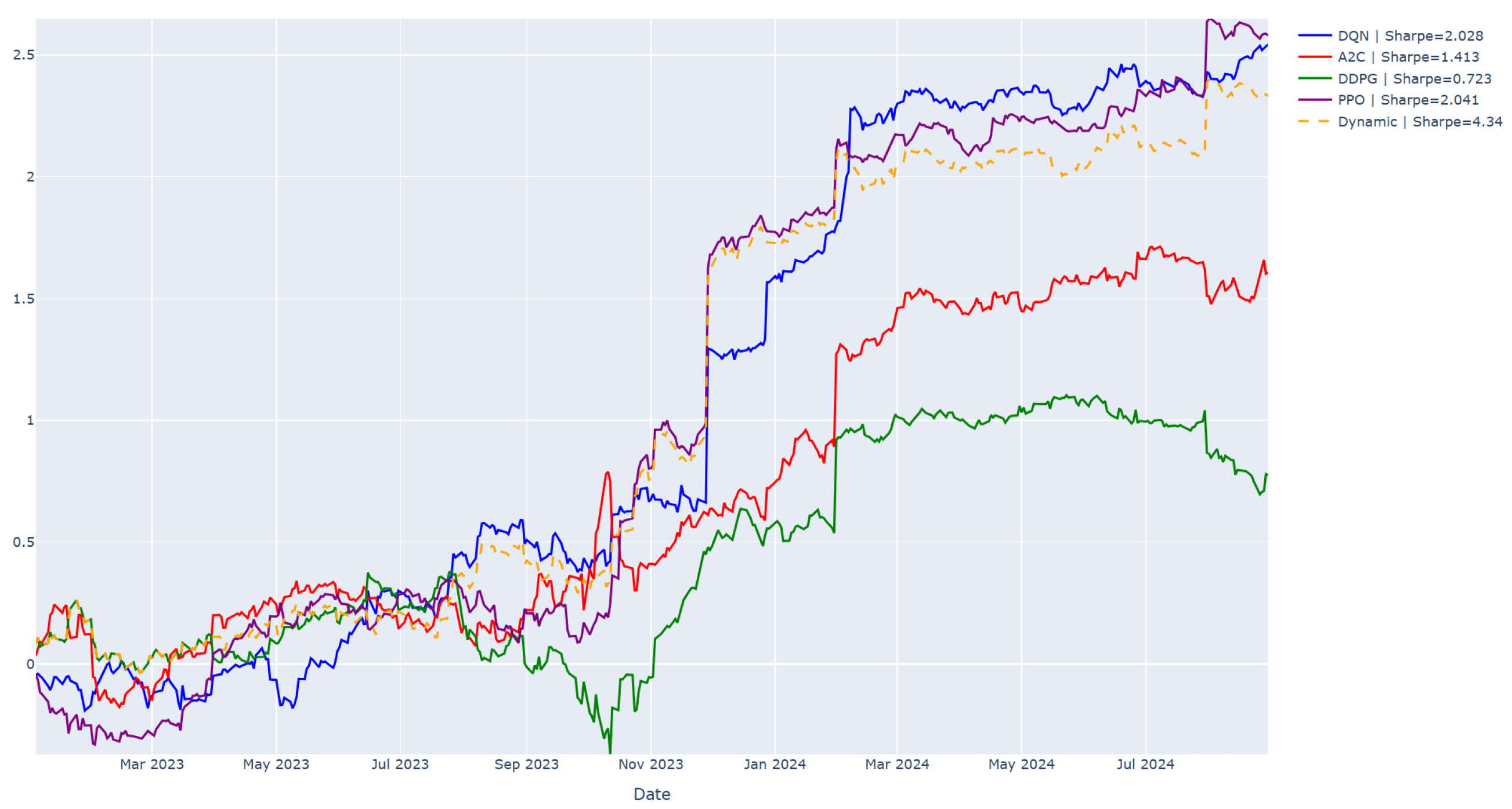
Dynamic (ART-DRL)	4.340	57.766	19.17	1.353	0.256

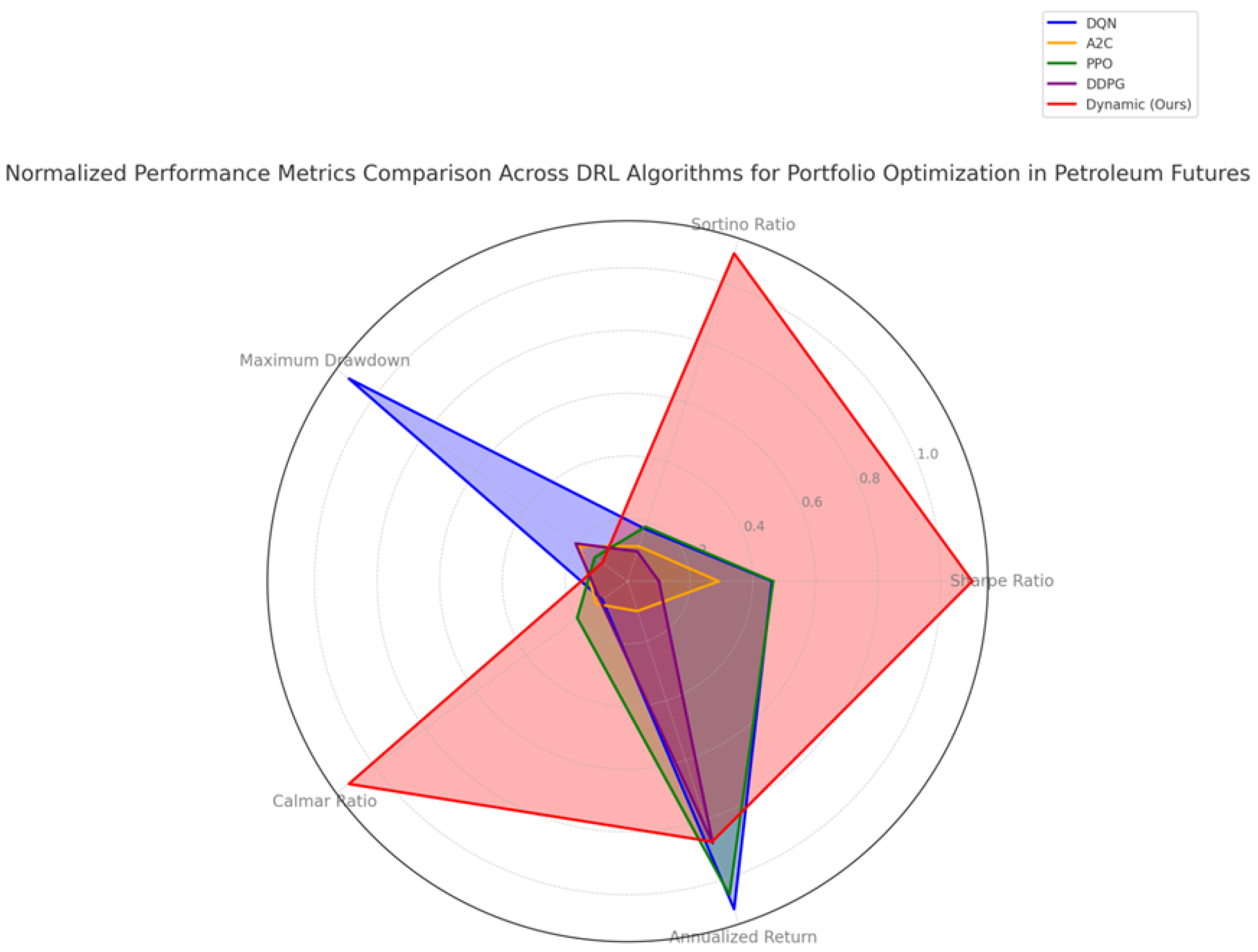
and Figure 4 present the performance of the Dynamic model. While Figure 4 shows that the Dynamic model did not achieve the highest cumulative PnL return by the end of the testing period (trailing DQN and PPO slightly), Figure 5 highlights its superior consistency and loss control. Unlike other models, the Dynamic strategy maintains a steady performance above the zero line, indicating resilience during adverse conditions. More holistically, Figure 5 compares all models using normalized performance metrics. The red-shaded region, representing the Dynamic model, shows the broadest reach across the Sharpe, Sortino, and Calmar ratios, as well as maximum drawdown, illustrating its strong risk-adjusted profile. This visual confirms the Dynamic model’s ability to strike a better balance between return and risk compared to any single-agent model. With a Sharpe Ratio of 4.340 and a Sortino Ratio of 57.766—far exceeding its peers—the Dynamic model excels in downside protection. Its low maximum drawdown (0.256) reflects robust risk control, making it well suited for adaptive trading environments. Even though its final cumulative return is slightly lower, its consistent risk-adjusted performance justifies its strength as a high-quality, adaptive strategy.

5.4. Model Evaluation

Table 4. Summary of model development methods.

Method	Strengths	Weaknesses
Method 1:
Single Agent	Simple Setup. Easy to compare agents. Learns basic risk-return trade-offs.	Poor adaptability. No agent switching. Unstable profits.
Method 2:
Multiple Agents	Better Adaptability. It uses discrete actions. Captures market patterns.	Higher complexity. It needs careful tuning. Some agents remain unstable.
Method 3:
Adaptive Switching
(ART-DRL)	Best risk-adjusted returns. Strong stability. Resilient in shocks.	Slightly lower cumulative return vs. DQN/PPO. More complex. Needs monitoring.

compares the three model development methods, highlighting their main strengths and weaknesses. The adaptive switching (ART-DRL) method offers the best risk-adjusted performance, while single-agent and multi-agent methods face limitations in adaptability and stability.

Table 5. Quantitative results of model methods.

Method	Sharpe	Sortino	Calmar	Ann. Return
Method 1
(best agent)	0.525 (PPO)	2125.8 (DDPG)	160.34 (DDPG)	−0.0395 (DDPG)
Method 2
(best agent)	2.041 (PPO)	5.734 (PPO)	1.977 (PPO)	1.476 (DQN)
Method 3
(ART-DRL)	4.340	57.77	19.17	1.353

presents the quantitative results of the three methods, showing that the adaptive switching approach (ART-DRL) achieves the best overall risk-adjusted performance.

• Method 1: Single Agent Trains each agent (DQN, PPO, A2C, DDPG) separately. Best Sharpe Ratio: 0.525 (PPO). Annualized return is negative.
• Method 2: Independent Agents Runs agents with discrete actions and a Transformer. Best Sharpe Ratio: 2.041 (PPO). Best annualized return: 1.476 (DQN).
• Method 3: Adaptive Switching (ART-DRL) Dynamically switches between agents based on recent performance. Sharpe Ratio: 4.340, Sortino Ratio: 57.77, Calmar Ratio: 19.17, Annualized return: 1.353.

While Method 2 delivers the highest annualized return, ART-DRL provides the best balance of return and stability.

5.5. Sensitivity Analysis and Parameter Robustness

To assess the robustness of the proposed ART-DRL framework, we conducted sensitivity analyses across two key dimensions: the training/testing data splits and the configuration of core hyperparameters. These analyses help evaluate how changes in modeling assumptions affect the performance of each method, particularly the dynamic Method 3 (ART-DRL).

To encourage long-term reward maximization, Method 1 employs a high discount factor ($\gamma =0.99$). Method 2 and Method 3 use $\gamma =0.01$ to prioritize short-term decision-making under frequent market fluctuations.

Transaction costs are explicitly modeled in Method 2 and Method 3 through a rebalancing penalty proportional to asset weight changes. While Method 1 does not include such costs, its underperformance renders the omission negligible for comparative purposes.

5.5.1. Training vs. Testing Splits

We varied the train–test split to investigate the influence of historical context length on model generalization. The default configuration employed a 90:10 split, using data from January 2014 to January 2023 for training and from February 2023 to January 2024 for testing. We additionally tested 80:20 and 70:30 splits.

Results demonstrated that Method 3 (ART-DRL) consistently maintained superior performance in risk-adjusted metrics such as the Sharpe, Sortino, and Calmar ratios across all splits. The robustness of Method 3 suggests that its performance-switching strategy effectively adapts to limited historical context without significant loss of generalizability.

5.5.2. Hyperparameter Variations

We performed controlled experiments by adjusting key hyperparameters in the reward function and agent design:

• Calmar reward weight ($\alpha$): {0.001, 0.005, 0.01}
• Volatility penalty weight ($\beta$): {0.8, 0.9, 0.95}
• Discount factor ($\gamma$): {0.01, 0.1, 0.99}

Table 6. Sensitivity analysis of ART-DRL under different configurations.

Configuration	Sharpe	Cum. Return (%)	Sortino	Ann. Return (%)
$\alpha =0.005,\beta =0.95,\gamma =0.01$ (default)	4.340	57.77	19.17	1.353
$\alpha =0.001,\beta =0.90,\gamma =0.01$	4.219	56.91	18.43	1.321
$\alpha =0.010,\beta =0.80,\gamma =0.10$	4.105	55.76	17.80	1.295
$\alpha =0.005,\beta =0.95,\gamma =0.99$	3.988	54.22	17.15	1.271

summarizes the effect of these variations on key evaluation metrics. Results indicate that:

• Increasing $\beta$ improves the agent’s ability to manage volatility.
• Lower $\gamma$ values promote short-term reactivity, which benefits intra-day learning in Methods 2 and 3.
• Method 3 outperforms across all tested parameter combinations, reflecting its flexibility in volatile, non-stationary environments.

5.5.3. Discussion

The sensitivity analysis reinforces the robustness of the ART-DRL approach across different modeling configurations. While performance varies slightly with parameter changes, the dynamic model’s agent-switching mechanism consistently identifies strategies that yield superior risk-adjusted returns. This supports our core hypothesis: adaptability, rather than fixed policy optimization, is critical in navigating the structural volatility of commodity futures markets.

6. Conclusions and Future Work

This study introduces a novel adaptive deep reinforcement learning framework—ART-DRL—for portfolio optimization in commodity futures markets. The framework integrates multiple DRL agents with a performance-driven switching mechanism and leverages a Transformer-based temporal encoder to capture the sequential dependencies and nonlinear dynamics inherent in petroleum derivatives trading.

Among the three strategies evaluated, Method 3 (ART-DRL) consistently outperformed the others on risk-adjusted metrics, achieving the highest Sharpe, Sortino, and Calmar ratios. These metrics highlight its ability to maintain favorable returns while managing volatility and downside risk. In contrast, Method 1 attained the highest cumulative return but suffered from significant volatility and poor drawdown control. Method 2 demonstrated a more balanced profile by incorporating transaction cost sensitivity and producing stable returns under diverse market conditions. These results highlight the effectiveness of adaptive agent-switching mechanisms, particularly in markets characterized by structural volatility and frequent regime shifts.

Our findings emphasize the importance of dynamic, risk-sensitive strategies in managing commodity futures portfolios. The ART-DRL model showed consistent resilience during periods of elevated uncertainty, including the 2023 energy price shocks. By benchmarking against a passive buy-and-hold strategy, we demonstrate the practical value of an adaptive policy selection framework that can adjust to evolving market regimes. These insights contribute meaningfully to the reinforcement learning literature in finance and offer concrete value to practitioners navigating real-world trading environments.

More broadly, our results support a fundamental insight: in dynamic financial markets, no single model maintains superiority across all conditions. Instead, adaptability—embodied in ART-DRL’s real-time agent selection—is key. The ability to dynamically choose among competing policies based on recent performance represents a significant advancement toward practical, self-adjusting trading systems. For traders, asset managers, and researchers, such adaptability offers a clear advantage in managing non-stationary and high-noise environments, especially in volatile markets like energy futures.

Beyond empirical performance, this work advances a conceptual shift—from optimizing a single static model to optimizing the selection and integration of multiple models. This meta-level optimization is especially relevant in commodity markets, where structural features such as seasonality, supply disruptions, and geopolitical uncertainty frequently alter return distributions and market behavior.

We acknowledge several limitations. Notably, this study does not explicitly address futures contract roll mechanics, expiration-induced volatility, or liquidity constraints—factors that can materially influence trading decisions and model robustness. Addressing these complexities is essential for transitioning from simulation to real-world deployment.

To that end, future research will focus on:

• Incorporating maturity-aware features and time-to-expiration adjustments;
• Enhancing volatility-sensitive learning components;
• Extending the framework to support multi-asset hedging and futures contract roll management;
• Collaborating with industry partners to better align the modeling approach with operational constraints and real-world execution challenges.

We hope this work encourages further exploration of adaptive AI systems in financial markets and fosters collaboration between academia and industry in developing robust, risk-aware trading strategies for complex, data-rich environments.

References

- Abuqaddom, I., Mahafzah, B., & Faris, H. (2021). Oriented stochastic loss descent algorithm to train very deep multi-layer neural networks without vanishing gradients. Knowledge-Based Systems, 230, 107391. [Google Scholar] [CrossRef]
- Bahoo, S., Cucculelli, M., Goga, X., & Mondolo, J. (2024). Artificial intelligence in finance: A comprehensive review through bibliometric and content analysis. SN Business & Economics, 4, 23. [Google Scholar] [CrossRef]
- Bao, W., Liu, B., & Zhang, J. (2019). A multi-agent reinforcement learning approach for stock trading. Expert Systems with Applications, 123, 306–327. [Google Scholar] [CrossRef]
- Buehler, H., Gonon, L., Teichmann, J., & Wood, B. (2019). Deep hedging. Quantitative Finance, 19(8), 1271–1291. [Google Scholar] [CrossRef]
- Chen, L., Lu, K., Rajeswaran, A., Lee, K., Grover, A., & Mordatch, I. (2021). Decision transformer: Reinforcement learning via sequence modeling. In M. Ranzato, A. Beygelzimer, Y. Dauphin, P. Liang, & J. Vaughan (Eds.), Advances in neural information processing systems (Vol. 34, pp. 15084–15097). Curran Associates, Inc. Available online: https://proceedings.neurips.cc/paper_files/paper/2021/file/7f489f642a0ddb10272b5c31057f0663-Paper.pdf (accessed on 20 June 2025).
- Deng, Y., Bao, F., Kong, Y., Ren, Z., & Dai, Q. (2016). Deep direct reinforcement learning for financial signal representation and trading. IEEE Transactions on Neural Networks and Learning Systems, 28(3), 653–664. [Google Scholar] [CrossRef] [PubMed]
- Du, Y., Tang, K., & Chen, K. (2023). A novel crude oil futures trading strategy based on volume-price time-frequency decomposition with ensemble deep reinforcement learning. Energy, 285, 128474. [Google Scholar] [CrossRef]
- Fu, R., Duan, Y., Liu, L., & Tan, W. (2025, May 14–16). Enhancing financial education with AI-driven learning and simulations. 2025 International Conference on Artificial Intelligence and Education (ICAIE 2025), Suzhou, China. [Google Scholar]
- Ganesh, J., & Rakheja, T. (2018, November 18–21). Reinforcement learning for optimized trade execution. 2018 IEEE Symposium Series on Computational Intelligence (SSCI) (pp. 526–533), Bangalore, India. [Google Scholar] [CrossRef]
- Hambly, B., Xu, R., & Yang, H. (2023). Recent advances in reinforcement learning in finance. Mathematical Finance, 33(3), 437–503. [Google Scholar] [CrossRef]
- Jaffri, A., Shirvani, A., Jha, A., Rachev, S., & Fabozzi, F. (2025). Optimizing portfolios with Pakistan-exposed exchange-traded funds: Risk and performance insight. Journal of Risk and Financial Management, 18(3), 158. [Google Scholar] [CrossRef]
- Jiajie, W., & Liu, L. (2025). Portfolio optimization through a multi-modal deep reinforcement learning framework. Engineering Open Access, 3(4), 1–8. [Google Scholar] [CrossRef]
- Koratamaddi, P., Wadhwani, K., Gupta, M., & Sanjeevi, S. (2021). Market sentiment-aware deep reinforcement learning approach for stock portfolio allocation. Engineering Science and Technology, an International Journal, 24, 848–859. [Google Scholar] [CrossRef]
- Lillicrap, T., Hunt, J., Pritzel, A., Heess, N., Erez, T., Tassa, Y., Silver, D., & Wierstra, D. (2015). Continuous control with deep reinforcement learning. arXiv, arXiv:1509.02971. [Google Scholar] [CrossRef]
- Massahi, M., & Mahootchi, M. (2024). A deep Q-learning-based algorithmic trading system for commodity futures markets. Expert Systems with Applications, 237, 121639. [Google Scholar] [CrossRef]
- Mnih, V. (2013). Playing Atari with deep reinforcement learning. arXiv, arXiv:1312.5602. [Google Scholar] [CrossRef]
- Mnih, V., Badia, A., Mirza, M., Graves, A., Lillicrap, T., Harley, T., Silver, D., & Kavukcuoglu, K. (2016, June 19–24). Asynchronous methods for deep reinforcement learning. 33rd International Conference on Machine Learning (Vol. 48, pp. 1928–1937), New York, NY, USA. [Google Scholar]
- Moody, J., & Saffell, M. (2001). Learning to trade via direct reinforcement. IEEE Transactions on Neural Networks, 12(4), 875–889. [Google Scholar] [CrossRef]
- Mousavi, B., Mahootchi, M., & Massahi, M. (2024). Developing a two-stage multi-period stochastic model for asset and liability management: A real case study in a commercial bank of Iran. Scientia Iranica, 31(22), 2148–2165. [Google Scholar] [CrossRef]
- Nan, L., Wang, J., & Xu, Y. (2020). Sentiment-aware deep reinforcement learning for algorithmic trading. Expert Systems with Applications, 163, 113716. [Google Scholar] [CrossRef]
- Parisotto, E., & Salakhutdinov, R. (2020, July 13–18). Stabilizing transformers for reinforcement learning. International Conference on Machine Learning (ICML), Online. [Google Scholar]
- Schulman, J., Wolski, F., Dhariwal, P., Radford, A., & Klimov, O. (2017). Proximal policy optimization algorithms. arXiv, arXiv:1707.06347. [Google Scholar] [CrossRef]
- Shakya, A., Pillai, G., & Chakrabarty, S. (2023). Reinforcement learning algorithms: A brief survey. Expert Systems with Applications, 231, 120495. [Google Scholar] [CrossRef]
- Vaswani, A., Shazeer, N., Parmar, N., Uszkoreit, J., Jones, L., Gomez, A., Kaiser, L., & Polosukhin, I. (2017, December 4–9). Attention is all you need. Advances in Neural Information Processing Systems (Vol. 30, ), Long Beach, CA, USA. [Google Scholar]
- Yang, H., Liu, X.-Y., Zhong, S., & Walid, A. (2020). Deep reinforcement learning for automated stock trading: An ensemble strategy. IEEE Computational Intelligence Magazine, 15(4), 73–83. [Google Scholar]
- Zhang, Y., Zohren, S., & Roberts, S. (2020). Deep reinforcement learning for trading strategies. Quantitative Finance, 20(9), 1459–1473. [Google Scholar]