Article

The Feedback Effects of Sovereign Debt in a Country’s Economic System: A Model and Application

1
Department of Management and Quantitative, College of Business Administration (COBA), Al Yamamah University, 7010 King Fahd Road, Al Qirawan, Riyadh 13541, Saudi Arabia
2
Portsmouth Business School, School of Accounting, Economics and Finance, Richmond Building, University of Portsmouth, Portland Street, Portsmouth PO1 3DE, UK
3
Carson College of Business, Washington State University, Pullman, WA 99163, USA
*
Author to whom correspondence should be addressed.
J. Risk Financial Manag. 2025, 18(6), 302; https://doi.org/10.3390/jrfm18060302
Submission received: 10 April 2025 / Revised: 18 May 2025 / Accepted: 23 May 2025 / Published: 1 June 2025
(This article belongs to the Special Issue Lending, Credit Risk and Financial Management)

Abstract

:
Many of the existing theoretical and empirical studies ignore the two-way relationship between a sovereign’s credit risk and economy. To address this gap, we develop a theoretical model that incorporates the feedback effects of sovereign-debt credit risk on a country’s economy and then provide empirical implications. The model links the risks of sovereign debt and economic fundamentals through a two-way transmission mechanism. In doing so, it demonstrates how economic-fundamentals-driven sovereign-debt credit risk can have a significant impact on economic fundamentals through a feedback effect that has the potential to significantly raise the sensitivity of a country’s economic performance to shocks from both the credit risk associated with sovereign debt and economic fundamentals. The outcomes of the theoretical model are then verified by empirically testing the feedback effects using a structural equation model (SEM) framework on data covering sovereign debt defaults worldwide. We demonstrate how disregarding feedback effects may result in information that is insufficient and less helpful to public-debt-management policymakers.

1. Introduction

The Global Financial Crisis threatened business development and growth. During this crisis, business growth rates fell, unemployment rose sharply, and poverty deepened. The financial crisis rolled back the hard-earned development gains of the previous several decades (Bernstein, 2017; Benbouzid et al., 2017; Schoenmaker, 2019). An understanding of the causes of financial crises is crucial from the perspectives of government, fiscal, and monetary policies. Specifically, a key question is whether the financial crisis was triggered by the credit risk or by the shocks to economic fundamentals. When considering the current economic slowdown, the US–China trade war, and the debt crisis in Europe, Africa, and Latin America, it is important and timely to review the debate on the causes of the Great Depression in relation to fiscal and monetary policies. For example, some commentators argue that a broad-based financial panic, including runs on wholesale funding and indiscriminate fire sales of even non-mortgage credit, choked the credit supply, thus pushing the economy into a much more severe decline than would have otherwise occurred (Bernanke, 2018). On the other hand, some do not accept the ‘transmission mechanism’—the way in which the financial shock is supposed to have affected actual spending to the extent necessary to justify a finance-first account of the slump. Similar to Baker (2018), these commentators hold that the bursting of the housing bubble was the main factor in the slump, with financial disruption being a minor and transitory factor. However, both sides seem to agree that current credit risk models do not adequately account for the transmission mechanism—i.e., the effects of credit-market conditions on real sector activity. In this paper, we aim to fill this gap by introducing an analytical model, which we empirically test using a SEM framework that can easily accommodate feedback effects.
The above debate reflects the two views in the literature on the major channels leading to financial crisis. One view argues that serious fundamental economic shocks shook financial institutions and markets, leading to a chain of insolvency among financial institutions and triggering a financial crisis (see Taylor, 2009; Taylor & Williams, 2009; Reinhart & Rogoff, 2011a, 2011b; Chen, 2013). The other view argues that the risks were transmitted in the opposite direction; the financial risks propagated through liquidity shocks and were amplified by contagion and ‘fear’ before spreading to economic fundamentals, which deteriorated and triggered a financial crisis (see Allen & Gale, 2000; Brunnermeier & Pedersen, 2009; Ang & Longstaff, 2013; Gennaioli et al., 2015; Acemoglu et al., 2015).
The events during and after the last global financial crisis, in 2008, and the subsequent European sovereign debt crisis, in 2012, have raised deep concerns about the rapidly growing level of sovereign debt and related credit risk in the global financial market. With the events surrounding Greece and Spain (Cencini, 2017) and then Ireland, Portugal, and Italy, the issue of sovereign credit risk is once again occupying the minds of academics, policymakers, and participants in financial markets. Significant government spending on health care and related borrowing after COVID-19 have also highlighted the increased indebtedness of sovereigns. Hence, given the sheer size of the sovereign debt market, it is important to understand the nature of sovereign credit risk, whether the financial risks of sovereign debt or economic fundamentals are the main causes of crises, and which of the following policies are effective: austerity, which aims to reduce debt, or stimulation of the economy (see, for example, Acharya et al., 2012; Glover & Richards-Shubik, 2014; Giglio et al., 2016).
More importantly, the two sides in the debate on the causes of financial crisis do not disagree on the interactions between economic fundamentals and financial markets. The effect of macroeconomic performance on risk premia and the counter-cyclical variation within have been documented in the literature (Fama & French, 1989; Campbell & Cochrane, 1999; Reinhart & Rogoff, 2011b). However, it is not so clear how credit risk is transmitted down to economic fundamentals. In this paper and as stated before, we develop a model to capture this downward transmission and then, subsequently, empirically test it.
Our theoretical model is built upon the structural model developed by Leland and Toft, which derives the credit risk of a firm when the firm’s asset value follows a diffusion process (see Leland, 1994; Leland & Toft, 1996; Chen, 2013). The framework and techniques developed by Leland and Taft (1996) and Chen (2013) derive the sovereign-debt credit risk of a country from the country’s GDP, but they also state that the credit risk does not affect the country’s GDP. In our model, the relationship between economic fundamentals and sovereign credit is two-way; sovereign credit risk affects a country’s economy too. To our knowledge, this paper represents the first effort to develop an analytical model that considers this feedback effect, and it explores the implications of this two-way transmission mechanism.
Furthermore, an economy consists of the real economy and the financial system. The real economy includes production (GDP), consumption, capital goods, labor, etc., while the financial system refers to financial assets, such as debt, equity, and currencies, among others. Our paper focuses on the feedback effect, which is a key factor that leads to financial crisis. Although the paper does not specifically analyze the 2007–2008 Financial Crisis, and southern European countries’ financial problems, feedback plays a key role in all those cases. During the 2007–2008 Financial Crisis, households’ defaults on mortgages created bank losses, and banks tightened their loans to households and firms. Being unable to rollover loans led to more mortgage defaults and firm layoffs. The feedback created a vicious cycle, resulting in the financial and economic crisis.
Empirically, since the 2008 Financial Crisis, there has been a regular stream of studies investigating the determinants of sovereign debt defaults. Among some of the most influential studies in this regard are Cuadra and Sapriza (2008), Sturzenegger and Zettelmeyer (2008), Manasse and Roubini (2009), Panizza et al. (2009), Van Rijckeghem and Weder (2009), Reinhart and Rogoff (2009, 2011a, 2011b), Hilscher and Nosbusch (2010), Trebesch (2019), and D’Erasmo and Mendoza (2021). However, a majority of these studies modeled sovereign default as a function of economic, financial, and political variables. Like the theoretical models, the feedback effect of debt default on these variables has largely been ignored. The feedback effect of sovereign debt defaults on economies (investment, exports, and GDP); public finance indicators, represented by the stock of debt, liquidity, and solvency; and the functioning of political systems (such as democratic conditions and elections) are seldom investigated and incorporated into the empirical modeling framework. This study helps fill this gap too by empirically modeling sovereign debt default using a structural equation model framework.
Using our theoretical model and comparing the comparative statistics with and without the feedback effects, we provide several findings and empirical implications that can contribute to the current literature. First and foremost, we find that a strong feedback effect can greatly increase the financial and economic risks and create a vicious cycle. Subsequently, by using a dataset that covers many sovereign debt defaults/crises across the globe, we empirically find that, in a number of cases, feedback effects do exist and are statistically significant. Furthermore, political system functioning affects social conditions, and social conditions impact the economy and financial system too. We conclude that these statistically significant interrelationships among economy, public finance, politics, and social sector are of interest and important for consideration in empirical modeling of sovereign debt defaults, as well as management of sovereign credit risk.
The remainder of this paper is organized as follows. Section 2 develops a two-way transmission model that incorporates the feedback effect from sovereign credit risk on a country’s GDP. Section 3 provides comparative statics and discusses the implications. Section 4 generalizes the model. Section 5 contains a discussion on the empirical testing of the feedback effects alongside the main findings. Finally, Section 6 summarizes and concludes the paper.

2. Theoretical Model

2.1. Feedback Effect of Sovereign Debt Risk on a Country’s GDP

The structural model developed by Merton (1974) has distinct advantages for linking a firm’s debt to its capital structure. This advantage has been applied to the relationship between a country’s GDP and the country’s sovereign debt (Minsky, 1992; Keen, 1995; Palley, 2009; Tse, 2001; Chen, 2013; Erdem & Yamak, 2014). The model enables us to determine endogenously the sovereign-debt credit spread from the country’s GDP. However, the existing structural model is an open system in which a country’s economy determines the sovereign-debt credit spread, but the country’s economy is not affected by the sovereign-debt credit risk. Our model considers the feedback effect of the sovereign-debt credit risk on a country’s GDP.
This feedback affects a country’s economy through two paths. First, the cost of the foreign debt that is borrowed by a country affects the country’s GDP as denominated by the foreign currency. The international Fisher effect states that differences in interest rates reflect expected changes in currency exchange rates among countries. The interest rate on sovereign debt is a factor that determines the exchange rate and, in turn, affects a country’s economy, as measured by the foreign currency. In addition to the exchange rate effect, secondarily, the interest rate on sovereign debt is a cost to the domestic economy. In this section, we focus on the first path and revisit the second path in Section 4, where we generalize the model.
Let there be two countries, denoted by i and j. Domestic debt refers to sovereign debt, which is denominated by a country’s domestic currency. Thus, domestic debt is independent of the currency exchange rate. A country’s GDP, Vni,t, follows a geometric Brownian motion with the growth rate, μ i , and volatility, σi.
d V n i , t = μ i V n i , t d t + σ i V n i , t d W i , t
where V n is the GDP measured by the domestic currency, and W is the standard Brownian motion (Wiener process). When country s is solvent, the domestic debt, F n V n i , t , as a financial claim on the country’s economy, satisfies the partial differential equation (Brennan & Schwartz, 1978; Leland, 1994; Leland & Toft, 1996; Dana, 2007)
μ i V n i , t V F n V n i , t + 1 2 σ i 2 V n i , t 2 2 V 2 F n V n i , t + C i r F n V n i , t = 0
The solution to Equation (1) is summarized in Appendix A.
We refer to a sovereign debt denominated by a foreign currency as a foreign debt for simplicity. The exchange rate, Q i , of the currency of country s, with respect to the reference currency, j, is characterized by the following process (Musiela & Rutkowski, 2006):
d Q i , t = r i , t r j , t Q i , t d t + σ Q i Q i , t d W i , t
Equation (2) is the stochastic version of the international Fisher effect; the differences in the nominal interest rates, r i , t r j , t , reflect the expected changes in the currency exchange rate between countries i and j. Country j, which lends money to country i, measures the GDP of country i with the currency j. The GDP of country i, as measured by the currency of country j, is given by the following:
d V i , t = μ i r i , t r j , t V i , t d t + σ i V i , t d W i , t
Assuming that the sovereign debt for country i is a consol bond with an annual coupon payment, C i 1 , the foreign sovereign debt is a financial claim on the country’s economy and satisfies the partial differential equation, as follows:
μ i r i , t r j , t V i , t V F V i , t + 1 2 σ i 2 V i , t 2 2 V 2 F n V i , t + C i r F V i , t = 0
The interest rate of a country depends on the value of the sovereign debt, F V i , t , and V i , t , and it is given by the following:
r i , t = S V i , t = C i F V i , t
To simplify the problem, we assume r i , t is the interest rate on the US dollar and is a constant.
Substituting (5) into (3), we obtain the following:
d V i , t = μ i C i F V i , t r j , t V i , t d t + σ i V i , t d W i , t
Substituting (5) into (4), we obtain the following:
μ i C i F V i , t r j , t V i , t V F V i , t + 1 2 σ i 2 V i , t 2 2 V 2 F n V i , t + C i r F V i , t = 0
The boundary conditions imposed to ensure that F V i , t is bounded and will not explode are as follows (Leland, 1994):
F V i , t C i r   a s   V i , t
where r is taken as the risk-free interest rate. Equation (7) requires an additional boundary condition. We impose the following condition as the default boundary:
F V i , t = γ B i   a t   V i , t = B i
where γ is the recovery rate at the sovereign debt default.1 Equation (9) implies that when the sovereign debt defaults, the lenders recover a fraction of the debt value, γ B i , where γ ≤ 1.

2.2. Subproblems

Compared with existing models (Leland, 1994; Leland & Toft, 1996; Chen, 2013), Equation (7) is no longer linear in F V i , t . To obtain a closed-form solution, we adopted the perturbation method; we first identified a small parameter, ϵ , and then expanded F V into a series, as follows:
F V = k = 0 ϵ k F k V ,
where we dropped the subscripts i and t to simplify the notations. The perturbation method breaks F V into F k V , k = 0, 1, 2…, which can be found one by one.

2.2.1. Boundary Conditions

The boundary conditions at the default boundary are as follows:
F 0 V + ϵ F 1 V + = γ B   a t   V = B
where they can be imposed on the zero-order and first-order subproblems, respectively, as follows:
F 0 B = γ B
F 1 B = 0
The debt becomes riskless as V approaches infinity, which implies the following:
F 0 V + ϵ F 1 V + C r   a t   V
The boundary conditions for the zero-order and the first-order subproblems are as follows, respectively:
F 0 V C r
F 1 V 0

2.2.2. Zero-Order Subproblem

To identify the small parameter, ϵ , we observe that when a country’s economy, V, goes to infinity, the sovereign debt approaches risk-free debt, as follows:
C F L V r 0
where F L V is the solution when V is large.2 Thus, we can define the following:
C F L V r = ϵ
Using the definition of ϵ, Equation (7) can be rewritten in terms of ϵ, as follows:
μ ϵ V V F L V + 1 2 σ 2 V 2 2 V 2 F L V + C i r F L V = 0
When V is large, we expand F L V as follows:
F L V = F L 0 V + ϵ F L 1 V +
We substitute (11) into (10) and ignore the terms of ϵ ; then, the zero-order subproblem becomes the following:
μ V V F L 0 V + 1 2 σ 2 V 2 2 V 2 F L 0 V = 0
Equation (12) has the general solution, as follows:
F L 0 V = a 3 + a 4 V Y + a 0 V
where a0 must be zero because F L 0 V cannot explode as V goes to infinity. Substituting the following:
F L 0 V = a 3 + a 4 V Y
into (12), we obtain the following:
Y = 2 μ σ 2 1
We observe that when C F V r = 0 , Equation (6) is a super martingale, which implies that the expected country’s economy is deteriorating, and V decreases to the default boundary, B. In this case, we expect that the country’s debt is much more sensitive to V than when V is very large. Hence, when a country’s debt is close to bankruptcy, the debt value is more sensitive to the change in GDP. We introduce a variable that amplifies the GDP scale when it is close to the default boundary, B, as follows:
u = ϵ m V B
and
d u = ϵ m d V
We introduce F S V as the solution when C F S V r ϵ . Under such conditions, Equation (7) can be rewritten using (16) as follows:
ϵ m + 1 u ϵ m + B u F S u + ϵ 2 m 1 2 σ 2 u ϵ m + B 2 2 u 2 F S u + C r F S u = 0
We expand FS(V) as follows:
F S V = F S 0 V + ϵ F S 1 V +
And we obtain the equation for F S 0 u , as follows:
1 2 σ 2 u 2 2 u 2 F S 0 u + C r F S 0 u = 0
where the solution to (20) satisfies the following:
F S 0 u = a 1 + a 2 u X
and
X = 8 r σ + 1
To match the inner solution (21) and the outer solution (14), we first apply the matching condition, as follows:
lim u a 1 + a 2 u X = lim V B a 3 + a 4 V Y
The right-hand side goes to a1 as V→B, which results in the following:
a 1 = a 3
Next, we combine the inner and outer solutions to cover the whole domain of V by subtracting the common parts of the two solutions. The common parts of the two solutions is the term that arises in the match process3, as follows:
F c o m m o n = a 1
After removing the common parts and substituting Equation (16), the solution that is valid over the whole domain of V is as follows:4
F 0 V = a 1 + a 2 ϵ m V B X + a 4 V Y
Applying the boundary condition F 0 V = C r as V goes to infinity, we obtain the following:
a 1 = C r
Applying the boundary condition F 0 B = γ B , we obtain the following:
a 4 = B Y C r γ B
Finally, the zero-order solution is as follows:
F 0 V = C r a ϵ V B X C r γ B V B Y
where we combine a 2 ϵ m X together to obtain a constant a ϵ .
To check the solution (24), we compute the numerical solution of the differential Equation (7), imposing the boundary conditions on Equations (8) and (9). The parameter values are provided in Table 1. Figure 1 compares Equation (24) with the numerical results. It shows that the zero-order solution captures the behavior of the sovereign debt well without the further complications of higher-order solutions.5

3. Comparative Statics and Implications

With the closed-form solution of Equation (24), we can conveniently derive the comparative statics. In Appendix A, we provide the solutions that ignore the feedback effects. These solutions represent a sovereign debt issued domestically (‘domestic debt’, for short). The comparative statics are summarized in Table 2.
The derivatives in the table are the comparative statics that provide the rates of changes; for example, F(V) represents debt and B the default boundary. Then dF(V)/dB is just the rate of change between the debt and the default boundary. The same interpretations apply to all derivatives in the table.
In parallel, we provide the comparative statics for the solutions that consider the feedback effects. These solutions represent a sovereign debt denominated by a foreign currency (‘foreign debt’, for short). The comparative statics are summarized in Table 3.

Empirical Implications

The comparative statics summarized in Table 2 and Table 3 provide rich empirical implications. In this section, we discuss some implications as examples. To make clear the implications, we need to make the parameters Y and Z more explicit, where Z is the parameter in the model without the feedback effect, and Y is the parameter in the model with the feedback effect.
Z = 1 σ 2 μ σ 2 2 + μ σ 2 2 2 + 2 r σ 2 1 σ i 2 μ i σ i 2 2 + μ i σ i 2 2 1 + 2 r σ i 2 μ i σ i 2 2 2
Using 1 + x 1 + x 2 for small x, we can rewrite as follows:
Z   2 μ σ 2 1 + r σ i 2 2 2 μ σ 2 1 = Y + 2 r σ 2 1 Y
which implies the following:
C r 2 1 V B Y < C r 2 1 V B Z < 0
which is as follows:
r F 0 < r F n < 0
In this case, F n is domestic debt (no borrowing from a foreign country), and F 0 is sovereign debt. Equation (25) implies that the market value of a sovereign debt is more sensitive to the risk-free interest rate if the feedback effect is considered. This implication is easy to understand. If the debt effect on GDP is ignored, the GDP is only affected by the risk-free interest rate indirectly through the decrease in the market value of the sovereign debt and the increase in the default probability of debt. When the feedback effect of the risk-free interest rate on the country’s economy is considered, a higher risk-free rate directly increases the interest rate payments and reduces the country’s GDP.
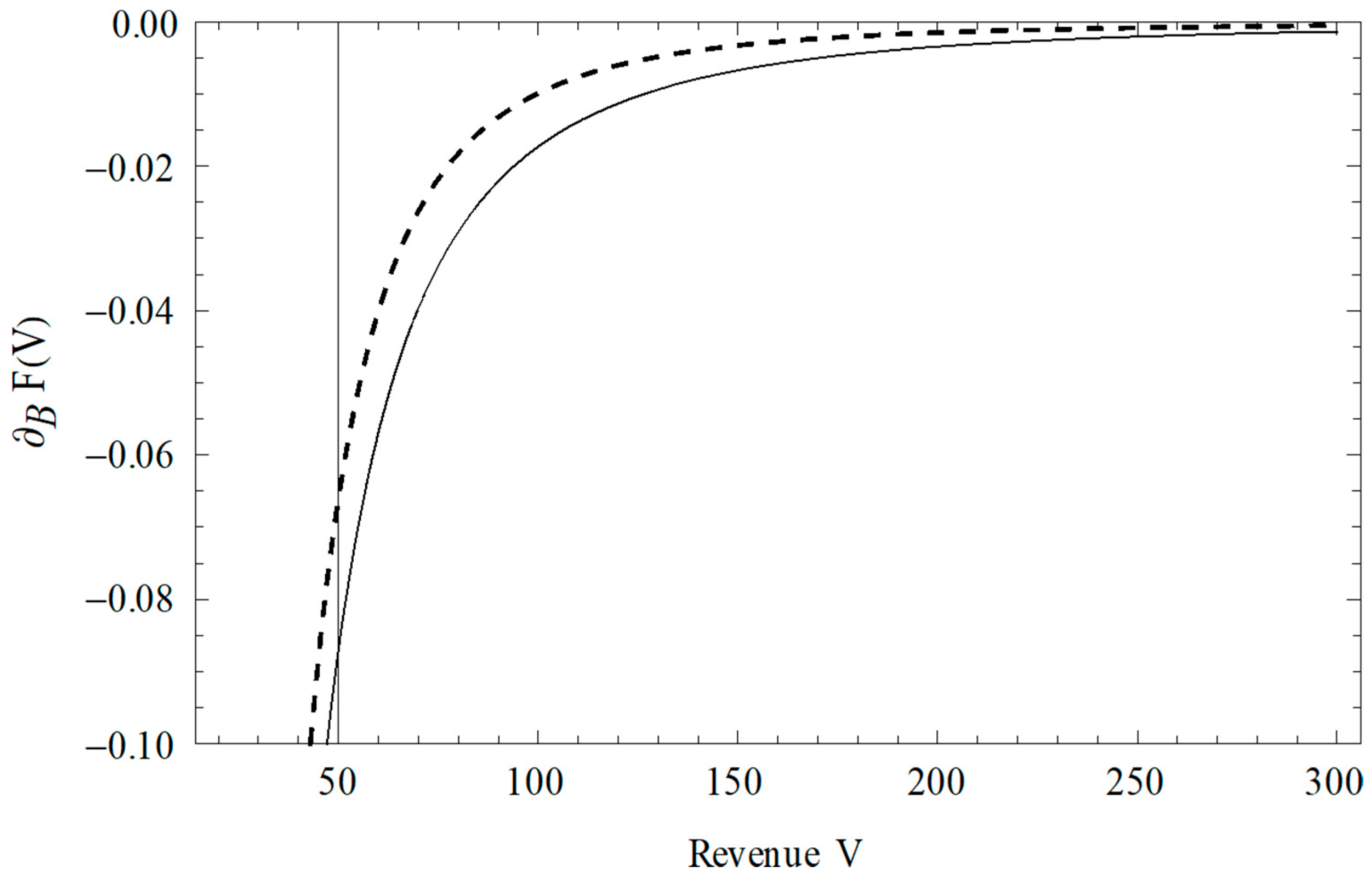
Similarly, we can compare the sensitivity of the country’s economy to other parameters. Figure 2 compares the sensitivity of the sovereign debt to the default boundary. It shows that the sensitivity that considers the feedback is higher than the sensitivity that ignores the feedback effect. This is particularly evident when the country’s economy is relatively low. For example, in Figure 2 the default boundary is assumed to be 15. When the country’s economy reaches 50, the sensitivity that ignores the feedback effect is about −0.07, while the sensitivity with the feedback is about −0.096.
The spread of the sovereign debt is given by the following:
S 0 V i , t = C F 0 ( V ) r = r 1 a e C r ( V B ) X 1 γ C r B V B Y r
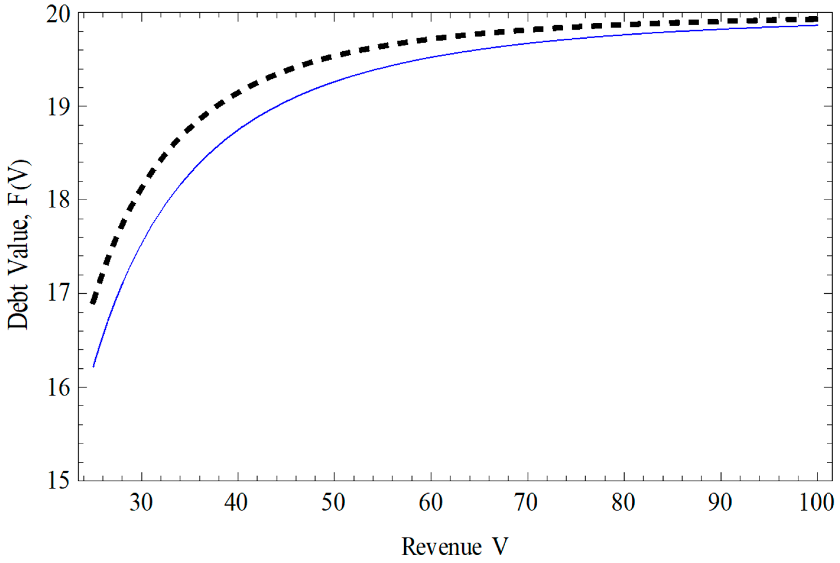
Figure 3 compares domestic debt to foreign debt. For a large GDP, V, the interest rate of the sovereign debt is close to the risk-free rate, and the exchange rate has little effect on the debt value. The value of domestic debt and the value of foreign debt are close. For a small GDP, the interest rate of the sovereign debt is higher than the risk-free rate and the domestic currency is expected to weaken. The weaker currency reduces the sovereign debt value denominated by the foreign currency. As shown in Figure 3, the lower the GDP, the larger the difference between the domestic debt and the foreign debt.
The comparative statics for the spread is
u S 0 = C F 0 ( V ) 2 u F 0 ( V )
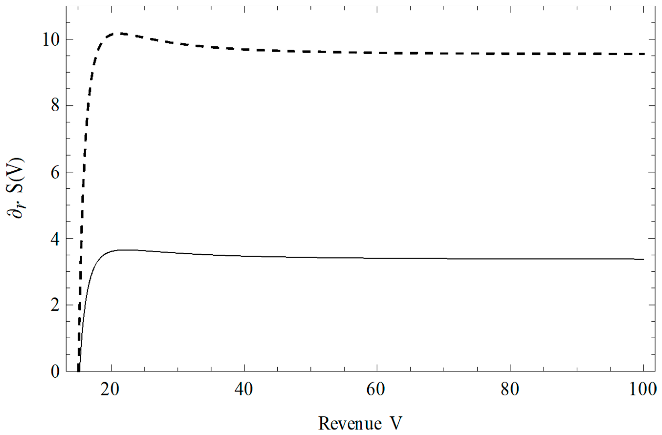
which has the opposite sign of the comparative statics of F0(V). This is an exception for the sensitivity of the spread to the risk-free interest rate, r, because the second term of r has a derivative of one in this case. Figure 4 compares the spread sensitivity to the risk-free interest rate between the domestic debt and foreign debt. It shows that both sensitivities to the risk-free interest rate are positive in both cases, while the foreign debt is less sensitive than the domestic debt. An increase in the interest rate of the US dollar strengthens the domestic currency through the international Fisher effect.7 This effect makes the spread of foreign debt less sensitive to the foreign interest rate.
The sensitivity of debt to shocks to economic fundamentals is an important measure of financial stability. Figure 5 shows that volatility has a negative effect on both domestic and foreign debt. The effect remains negative and approaches zero as V becomes large. The effect is much larger on the foreign debt than the domestic debt. When V is small, in addition to the negative effect of the GDP volatility on the debt, a small V weakens the domestic currency. The combined effect makes the foreign debt much more sensitive to volatility. A foreign debt can make the financial situation less stable than the same amount of domestic debt, when the country’s economy, V, is low.

4. Generalizing the Model

The previous model can be generalized to cover more cases. We introduce two indicator functions, a and b, in the stochastic process of a country’s GDP.
d V i , t = μ i a C F V i , t r j b C V i , t V i , t d t + σ i V i , t d W i , t
where
C V i , t = C F V i , t F V i , t V i , t
which is the product of the cost of debt and the debt-to-GDP ratio. Equation (27) covers the following cases in the GDP process:
  • a = 0, b = 0 GDP denominated by domestic currency and costs of debt ignored;
  • a = 1, b = 0 GDP denominated by a foreign currency and costs of debt ignored;
  • a = 0, b = 1 GDP denominated by domestic currency and costs of debt included;
  • a = 1, b = 1 GDP denominated by a foreign currency and costs of debt included.
Case 1 is the base model (see Appendix A). Case 2 is the model developed above. Cases 3 and 4 can be solved using the approach discussed above.

5. Empirical Evidence on Feedback Effects

5.1. Methodological Framework (Structural Equation Model of Feedback Effects)

A structural equation model is used to consider the feedback effect of debt defaults and measurement error in estimating the latent variables representative of the economy, public finances, political system functioning, and the social sector. We follow a number of authors, such as Ghulam (2025), Nakatani (2023), Rahman et al. (2023), and Mpapalika and Malikane (2019), among many others, in selecting some of these variables used in our study. We extend the theoretical model to accommodate the role of non-economic/financial factors in determining risk of default, as well as these factors being determined by risk of default themselves. The use of SEM in social science research is becoming increasingly popular due to its flexibility in dealing with simultaneity and feedbacks in relationships and its ability to deal with latent variables that are not available in a single measurable form. The feedback effect of sovereign debt default that we developed is easily accommodated in a SEM framework. We hypothesize and empirically test that debt defaults affect latent variables such as the economy (ECON), public finances (FINANC), and domestic political system functioning (POLITIC). Similarly, these latent variables—as well as the latent variable representative of the social sector (SOC)—are connected with each other. For example, politics affects investment in the social sector, the social sector affects the economy and public finances, and domestic politics affects both the economy and public finances.
The four latent variables (ECON, FINANC, POLITIC, and SOC) are determined by a number of country level variables. To test these hypotheses, we use data covering 107 countries from 1975 to 2019. More specifically, these data include East Asia and the Pacific (10), Europe and Central Asia (22), Latin America and the Caribbean (24), the Middle East and North Africa (8), South Asia (8), and Sub-Saharan Africa (35), where the numbers in brackets indicate region-specific sovereigns in the dataset. The data consist of 10.28%, 19.63%, 36.45%, and 33.64% of high-, low-, lower-middle-, and upper-middle-income countries.
Lagged GDP growth (gdpg_l); inflation (inf); exports, FDI, gross fixed capital formation growth rate (gfc_gr), and central government debt at level, as well as % of GDP (ex_gdp, fdi_gdp, and cgd_gdp); and exchange rate crisis (ex_cris), measured by a dummy variable when the local currency depreciates by more than 15% against the USD, determine the latent variable representative of the economic conditions index (ECON) of the country. Short term debt as a percentage of both the total public debt and reserves (sd_tdeb and sd_tres); reserves as a percentage of the total debt (res_deb); imports-to-GDP ratio (imp_gdp); real interest rate (rintr); debt service as a percentage of GDP (ds_gdp); and triple crisis (trip_cr), comprising banking, currency, and sovereign debt, all determine the latent variable approximating the index of public finance conditions (FINANC) of a sovereign. A dummy variable representing a finite term in office or not (f_ter), military expenditure as a % of GDP (milt), years since in office (y_of), and years left in the current term (y_cur) are used to explain the variations in the latent variable representing the political environment (POLITIC) of a country.
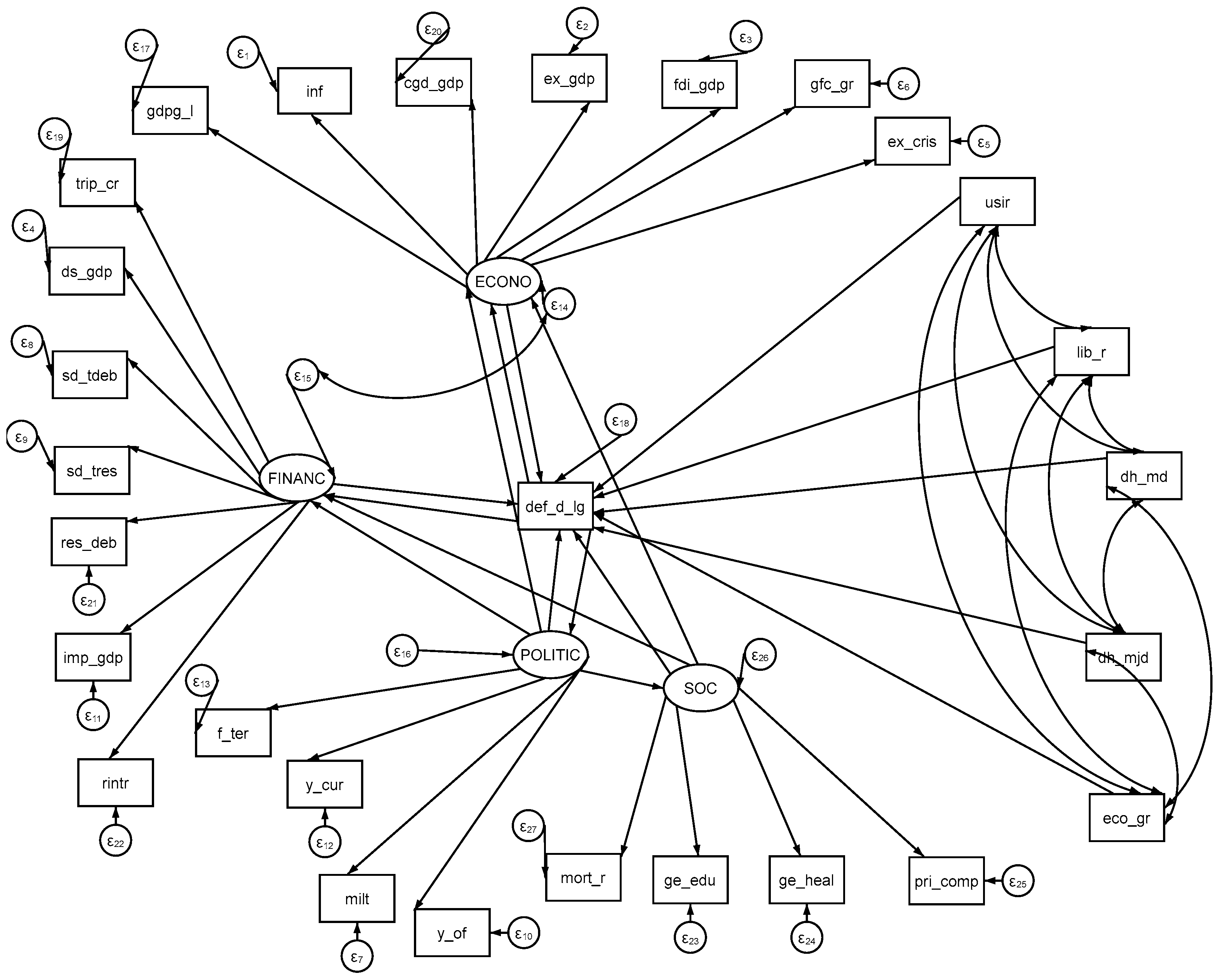
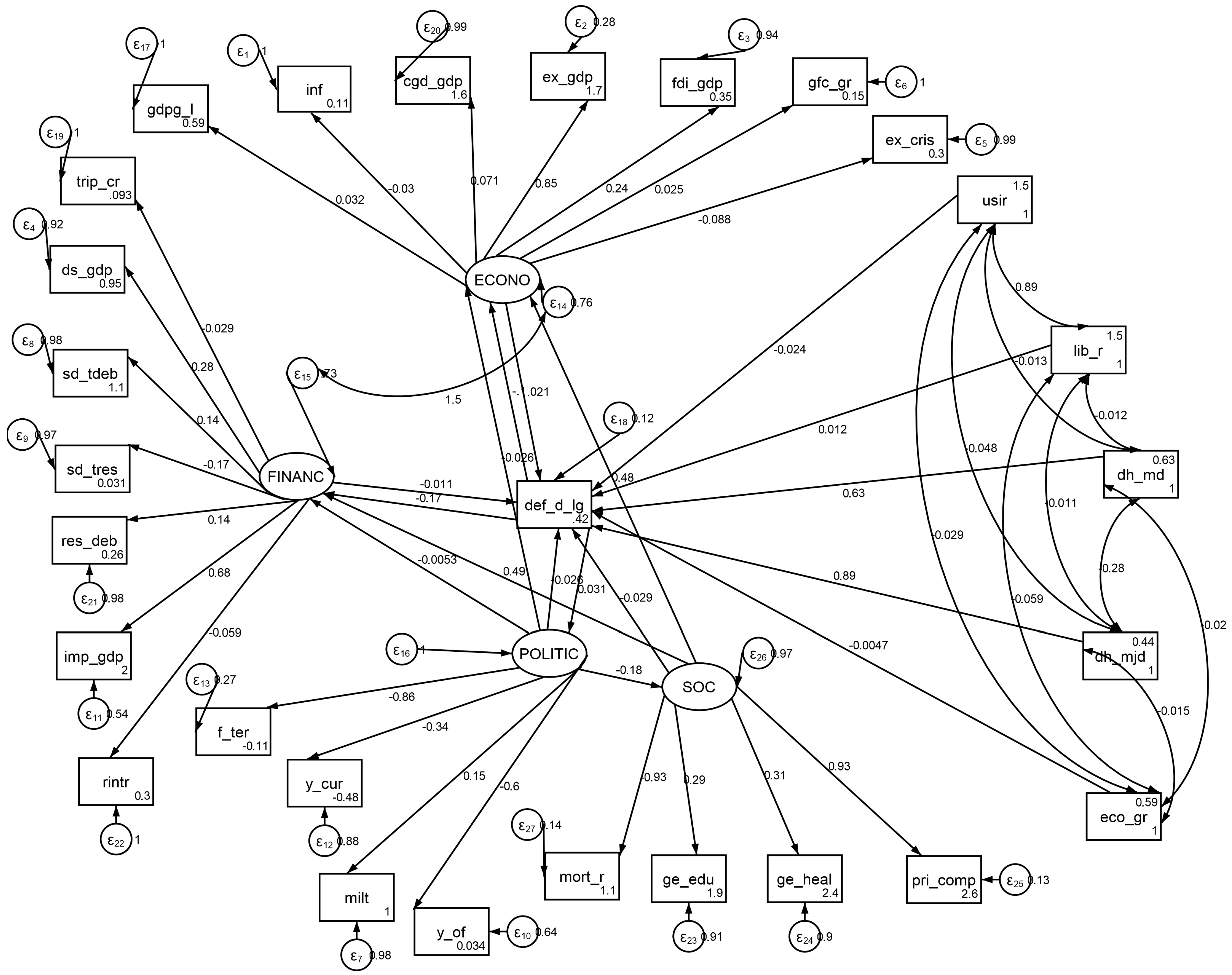
Lastly, a country’s expenditures on education and health as a percentage of GDP (ge_edu ge_heal), mortality rate (mort_r), and primary education competition rate (pri_comp) are used to approximate the last latent variable representative of the social sector development index (SOC). In addition, a few other variables, such as the US interest rate (usir), LIBOR rate (lib_r), current economic GDP growth rate (eco_gr), and two dummy variables of the default history of a sovereign (dh_md and dh_mjd), representative of the medium and higher levels of debt defaults (whereas moderate and high levels of arrears are defined as USD 50 million to <1 billion and USD ≥ 1 billion), are used as observed variables to explain the variations in sovereign debt defaults. Figure 6 depicts these interrelations/feedback effects of the sovereign debt risk, economic and financial conditions, politics, and social sector.

5.2. Data Sources and Detailed Description of Variables

The Bank of England’s and Canada’s databases on sovereign debt defaults are used to determine the debt default levels in log form (def_d_lg). Public finance- and economy-related data were extracted from the World Development Indicators (WDI) database. Political variables, including years in office and years left in the current term, as well as fixed-term dummy variables, were sourced from the Inter-American Development Bank’s database of political institutions. LIBOR and US interest rates are sourced from the database of the Federal Reserve. Table 4 contains the description of the variables used in our SEM framework.

5.3. Main Empirical Findings and Discussion

Looking at the SEM estimates presented in Table 5 and the path diagram (Figure 6), some salient observations can be made. Economic conditions, politics, and the social sector play important roles in determining the level of defaulted debt, but the same cannot be said in relation to public finances. A detailed analysis of the factor loading presented in Figure 7 indicates that the positive and statistically significant loading of cgd_gdp, gdpg_l, fdi_gdp, and ex_gdp is not sufficient to compensate for the negative loading of ex_cris and inf. Considering the feedback effect of defaulted debt on the economy, improving the index of economic activities does not guarantee a reduction in defaulted debt levels. On the other hand, increased values of the indices of political conditions and social sector/investment conditions reduce defaulted debt levels.
Except for military expenditures, the factor loading of all other political variables is negative and statistically significant. Similarly, for the social sector, except for mortality, the factor loading of all other variables is positive and statistically significant. More importantly, looking into the feedback effect, the level of defaulted debt contributes negatively to economic activity (thus a negative feedback effect on economic activity), while the development of the social sector contributes positively. The feedback effect of politics on the economy is not statistically significant. Defaulted debt levels also contribute negatively to public finance (again confirming a negative feedback effect) but positively to politics. Similarly, politics negatively impacts the social sector, but social sector development/conditions positively impact public finance conditions.
Broadly speaking, the analytical model and empirical findings indicate the existence of sovereigns’ defaults risk feedbacks and that accommodating the interrelationships and feedbacks of sovereign-debt default models could result in a more nuanced and potentially clearer understanding of the issue, as well as provide some directions for integrating these feedback effects into policy discourse.

6. Conclusions

Given the high level of sovereign debt and, in some cases, the resultant defaults, which have threatened businesses and the global economy, a fundamental question is whether sovereign credit risk or common shocks to macroeconomic fundamentals are the causes of financial crises and defaults. The existing structural model links the sovereign debt of a country to the country’s GDP. The model derives the credit spread when the country’s economy follows a Brownian motion, while the country’s economy is independent of the credit spread. This paper develops a theoretical model that incorporates the feedback effects of the sovereign-debt credit risk on a country’s GDP. Our model allows for the following two-way transmissions: from the GDP risk to the sovereign debt and the feedback from the debt credit risk to the country’s economy. The model shows that the feedback can have significant effects on the sovereign-debt credit risk. These feedback effects significantly increase the sensitivities of the sovereign debt to the shocks from both economic fundamentals and sovereign-debt credit premia. These findings have empirical implications for the transmission mechanism of risk between the sovereign debt of a country and the country’s economic fundamentals.
Our theoretical model focuses on the following two transmission mechanisms: the contraction of the country’s economy due to the costs of sovereign debt and the effect of the exchange rate on the foreign debt and GDP as measured by the foreign currency. Which effect—the costs of sovereign debt and the exchange rate—is more important depends on multiple factors. For example, the exchange rate can have positive or negative effects on debt. If the foreign interest rate is higher than the domestic interest rate, then the foreign currency depreciates and the domestic currency appreciates overtime. Then, for the consol bond in the model, the borrower benefits from the exchange rate. If the foreign interest rate is lower than the domestic interest rate, then the effect of the exchange rates reverses, and when the foreign interest rate and the domestic interest rate are the same, the exchange rate has no effect. Thus, the relative effects of the exchange rate and the cost of sovereign debt change with the exchange rate.
By using an SEM framework that can accommodate inter-relationships and feedback effects, our estimates confirm these feedback effects. In our empirical testing, rather than modeling only economy and credit risk measured by sovereign default, we tried to link and assess the feedbacks of sovereign defaults with economy, public finance, and the country’s politics and spending on the social sector. Hence, a theoretical and empirical model that is capable of answering the question of how financial risk is transmitted and how this causes financial crises must incorporate other transmission channels, such as runs on wholesale funding, fire sales, choked credit supply, and contagions. Such a model needs to introduce jump risks for credit premia and the interactions between multiple financial institutions, firms, and investors. The lack of inclusion of these transmission channels could be considered a limitation of this study. These challenging extensions will be explored in our future research work, nonetheless.

Author Contributions

Conceptualization, Y.G. and S.L.; methodology, Y.G. and S.L.; software, Y.G. and S.L.; validation, Y.G. and S.L.; formal analysis, Y.G. and S.L.; investigation, Y.G. and S.L.; resources, Y.G.; data curation, Y.G.; writing—S.L. and Y.G.; writing—review and editing, Y.G. and S.L.; visualization, Y.G.; supervision, Y.G.; project administration, Y.G.; funding acquisition, none. All authors have read and agreed to the published version of the manuscript.

Funding

This research received no external funding.

Institutional Review Board Statement

Not applicable.

Informed Consent Statement

Not applicable.

Data Availability Statement

Data is available upon request to the corresponding author.

Conflicts of Interest

The authors declare no conflict of interest.

Appendix A

Appendix A.1. A Domestic Debt

In this appendix, we use a structural model to establish the endogenous link between country credit spreads and economic fundamentals. As systemic risk originates from the financial crisis, we incorporate a jump risk process in the model to capture the sudden drastic shock that causes financial instability so widespread that it affects entire economic and financial systems. Let there be n countries denoted by i, with i = 1, 2, 3…, n, and i = 0 refers to the globe. Assume that a country’s economy, Vi,t, follows a stochastic process, which includes a geometric Brownian motion with average growth rate, μ ^ i , and volatility, σ i , as well as a jump process. More specifically, the country’s economy under the physical probability measure is characterized by the following process:
d V i , t = μ ^ i V i , t d t + σ i V i , t d W ^ i , t
where W ^ i , t is a standard Brownian motion.
Suppose that markets are complete, and there is a unique risk-neutral measure, P. Let
Z W , t = e x p θ W ^ i , t 1 2 θ 2 t d P d P ^ = Z W , t
under the risk-neutral measure,
d W 0 , t = d W ^ 0 , t θ d t
where θ is associated with the global economy (global GDP), which represents the systematic economic shock. The risk-neutral country’s economic process can be expressed as followed:
d V i , t = μ i V i , t d t + σ i V i , t d W i , t
where
μ i = μ ^ i θ ρ 0 i σ i = μ ^ i θ β i G D P σ i
and ρ 0 i is the correlation coefficient between W0,t and Wi,t. Assume that the sovereign debt for country i is a consol bond with a coupon rate Ci, F(Vi,t) is the market value of country i’s debt at time t, and r is the riskless rate. When country i is solvent, the claim on the county’s economy satisfies the following equation:
μ i V i , t t F V i , t + 1 2 σ i 2 V i , t 2 V 2 F V i , t + C i r F V i , t = 0
A country defaults on its debt whenever the country’s GDP falls below interest expense. This involves two situations. First, a default occurs due to the normal GDP shortfall and the country is unable to pay the interest of its debt. When the following boundary condition
V i , t < C i
is met, then country i defaults. Thus, (A1) is subject to the following default condition:
F C i = 0
An additional boundary condition is imposed to ensure that F(Vi,t) is bounded and will not explode (Leland, 1994)
F V i , t C i r   a s   V i , t
The value of debt F(Vi,t) is given by the following:
F V i , t = C i r 1 V i , t C i Z i
where Zi is the solution to
2 r Z i μ i Z i Z i 1 σ i 2 = 0
In (A2), the value of a country’s debt is equal to the present value of the consol minus the present value of the loss at default due to the shock to the country’s economic fundamentals.
Only the negative root satisfies the condition in (A3), which is as follows:
Z i = 1 σ i 2 μ i σ i 2 2 + μ i σ i 2 2 2 + 2 r σ i 2
The credit spread for country i’s consol is given by the following:
S V i , t = C i F V i , t r = r 1 V i , t C i Z i r

Notes

1
A government may not default its debt based on a fixed default boundary but makes a default decision optimally. The default boundary can be endogenously determined as an optimization problem (Leland, 1994; Leland & Toft, 1996). As a first step, we enforced this boundary condition for simplicity.
2
Fk(V) is the outer solution in the perturbation method.
3
The reason for this is that we do not want to double count the common parts in the composite solution.
4
This solution is the composite solution in the perturbation method.
5
Including higher order solutions can increase the accuracy further.
6
More specifically, assume the GDP is 50 (say billion), while the default boundary is 15 (billion) which is 30% of the GDP, a relatively less leveraged economy. With a USD 1 billion increase in the default boundary, −0.01 represents a USD 10 million reduction in the debt value. Thus, from −0.07 to −0.09 represents a USD 20 million loss in the debt value. Furthermore, the feedback is compounding on itself. In a simple discounting, it takes about 10 years for an initial value to be cut in half at −7% but takes about 8 years to cut in half at −9%.
7
This is true assuming the real interest rates are the same for domestic debt and foreign debt. If the real interest rates are different in the short run, then the international Fisher effect does not apply.

References

  1. Acemoglu, D., Ozdaglar, A., & Tahbaz-Salehi, A. (2015). Systemic risk and stability in financial networks. American Economic Review, 105(2), 564–608. [Google Scholar] [CrossRef]
  2. Acharya, V., Engle, R., & Richardson, M. (2012). Capital shortfall: A new approach to ranking and regulating systemic risks. American Economic Review, 102(3), 59–64. [Google Scholar] [CrossRef]
  3. Allen, F., & Gale, D. (2000). Financial contagion. Journal of Political Economy, 108(1), 1–33. [Google Scholar] [CrossRef]
  4. Ang, A., & Longstaff, F. A. (2013). Systemic sovereign credit risk: Lessons from the US and Europe. Journal of Monetary Economics, 60(5), 493–510. [Google Scholar] [CrossRef]
  5. Baker, D. (2018). The housing bubble and the great recession: Ten years later. Center for Economic and Policy Research. [Google Scholar]
  6. Benbouzid, N., Mallick, S. K., & Sousa, R. M. (2017). Do country-level financial structures explain bank-level CDS spreads? Journal of International Financial Markets, Institutions and Money, 48, 135–145. [Google Scholar] [CrossRef]
  7. Bernanke, B. S. (2018). The real effects of disrupted credit: Evidence from the global financial crisis. Brookings Papers on Economic Activity, 2018(2), 251–342. [Google Scholar] [CrossRef]
  8. Bernstein, S. (2017). The United Nations and the governance of sustainable development goals. In Governing through goals: Sustainable Development Goals as governance innovation (pp. 213–239). MIT Press. [Google Scholar]
  9. Brennan, M. J., & Schwartz, E. S. (1978). Corporate income taxes, valuation, and the problem of optimal capital structure. Journal of Business, 51, 103–114. [Google Scholar] [CrossRef]
  10. Brunnermeier, M. K., & Pedersen, L. H. (2009). Market liquidity and funding liquidity. The Review of Financial Studies, 22(6), 2201–2238. [Google Scholar] [CrossRef]
  11. Campbell, J. Y., & Cochrane, J. H. (1999). By force of habit: A consumption-based explanation of aggregate stock market behavior. Journal of Political Economy, 107(2), 205–251. [Google Scholar] [CrossRef]
  12. Cencini, A. (2017). The sovereign debt crisis: The case of Spain. Cuadernos de Economía, 40(112), 1–13. [Google Scholar] [CrossRef]
  13. Chen, H. (2013). Comment on “Systemic sovereign credit risk: Lessons from the US and Europe” by Ang and Longstaff. Journal of Monetary Economics, 60(5), 511–516. [Google Scholar] [CrossRef]
  14. Cuadra, G., & Sapriza, H. (2008). Sovereign default, interest rates and political uncertainty in emerging markets. Journal of International Economics, 76(1), 78–88. [Google Scholar] [CrossRef]
  15. Dana, R. A. (2007). Financial markets in continuous time. Springer. [Google Scholar]
  16. D’Erasmo, P., & Mendoza, E. G. (2021). History remembered: Optimal sovereign default on domestic and external debt. Journal of Monetary Economics, 117, 969–989. [Google Scholar] [CrossRef]
  17. Erdem, H. F., & Yamak, R. (2014). The dynamic relationship economics and financial instability. International Reviews Business Research Papers, 10(1), 39–48. [Google Scholar] [CrossRef]
  18. Fama, E. F., & French, K. R. (1989). Business conditions and expected returns on stocks and bonds. Journal of Financial Economics, 25(1), 23–49. [Google Scholar] [CrossRef]
  19. Gennaioli, N., Shleifer, A., & Vishny, R. (2015). Neglected risks: The psychology of financial crises. American Economic Review, 105(5), 310–314. [Google Scholar] [CrossRef]
  20. Ghulam, Y. (2025). A further examination of sovereign domestic and external debt defaults. The North American Journal of Economics and Finance, 76, 102322. [Google Scholar] [CrossRef]
  21. Giglio, S., Kelly, B., & Pruitt, S. (2016). Systemic risk and the macroeconomy: An empirical evaluation. Journal of Financial Economics, 119(3), 457–471. [Google Scholar] [CrossRef]
  22. Glover, B., & Richards-Shubik, S. (2014). Contagion in the European sovereign debt crisis (No. w20567). National Bureau of Economic Research. [Google Scholar]
  23. Hilscher, J., & Nosbusch, Y. (2010). Determinants of sovereign risk: Macroeconomic fundamentals and the pricing of sovereign debt. Review of Finance, 14(2), 235–262. [Google Scholar] [CrossRef]
  24. Keen, S. (1995). Finance and economic breakdown: Modeling Minsky’s “financial instability hypothesis”. Journal of Post Keynesian Economics, 17(4), 607–635. [Google Scholar] [CrossRef]
  25. Leland, H. E. (1994). Corporate debt value, bond covenants, and optimal capital structure. The Journal of Finance, 49(4), 1213–1252. [Google Scholar] [CrossRef]
  26. Leland, H. E., & Toft, K. B. (1996). Optimal capital structure, endogenous bankruptcy, and the term structure of credit spreads. The Journal of Finance, 51(3), 987–1019. [Google Scholar] [CrossRef]
  27. Manasse, P., & Roubini, N. (2009). “Rules of thumb” for sovereign debt crises. Journal of International Economics, 78(2), 192–205. [Google Scholar] [CrossRef]
  28. Merton, R. C. (1974). On the pricing of corporate debt: The risk structure of interest rates. The Journal of Finance, 29(2), 449–470. [Google Scholar]
  29. Minsky, H. P. (1992). The financial instability hypothesis (No. 74). Working paper. Levy Economics Institute of Bard College. [Google Scholar]
  30. Mpapalika, J., & Malikane, C. (2019). The determinants of sovereign risk premium in African countries. Journal of Risk and Financial Management, 12(1), 29. [Google Scholar] [CrossRef]
  31. Musiela, M., & Rutkowski, M. (2006). Martingale methods in financial modelling (Vol. 36). Springer Science & Business Media. [Google Scholar]
  32. Nakatani, R. (2023). Sovereign debt crisis and fiscal devolution. Journal of Risk and Financial Management, 17(1), 9. [Google Scholar] [CrossRef]
  33. Palley, T. I. (2009). The limits of Minsky’s financial instability hypothesis as an explanation of the crisis (No. 11/2009). IMK Working Paper. Hans-Böckler-Stiftung, Institut für Makroökonomie und Konjunkturforschung (IMK). [Google Scholar]
  34. Panizza, U., Sturzenegger, F., & Zettelmeyer, J. (2009). The economics and law of sovereign debt and default. Journal of Economic Literature, 47(3), 651–698. [Google Scholar] [CrossRef]
  35. Rahman, H. U., Arian, A., & Sands, J. (2023). Does fiscal consolidation affect non-performing loans? Global evidence from heavily indebted countries (HICs). Journal of Risk and Financial Management, 16(9), 417. [Google Scholar] [CrossRef]
  36. Reinhart, C. M., & Rogoff, K. S. (2009). This time is different: Eight centuries of financial folly. Princeton University Press. [Google Scholar]
  37. Reinhart, C. M., & Rogoff, K. S. (2011a). The forgotten history of domestic debt. The Economic Journal, 121(552), 319–350. [Google Scholar] [CrossRef]
  38. Reinhart, C. M., & Rogoff, K. S. (2011b). From financial crash to debt crisis. American Economic Review, 101(5), 1676–1706. [Google Scholar] [CrossRef]
  39. Schoenmaker, D. (2019). A framework for sustainable finance. Available online: https://papers.ssrn.com/sol3/papers.cfm?abstract_id=3125351 (accessed on 23 July 2023).
  40. Sturzenegger, F., & Zettelmeyer, J. (2008). Haircuts: Estimating investor losses in sovereign debt restructurings, 1998–2005. Journal of International Money and Finance, 27(5), 780–805. [Google Scholar] [CrossRef]
  41. Taylor, J. B. (2009). The financial crisis and the policy responses: An empirical analysis of what went wrong (No. w14631). National Bureau of Economic Research. [Google Scholar]
  42. Taylor, J. B., & Williams, J. C. (2009). A black swan in the money market. American Economic Journal: Macroeconomics, 1(1), 58–83. [Google Scholar] [CrossRef]
  43. Trebesch, C. (2019). Resolving sovereign debt crises: The role of political risk. Oxford Economic Papers, 71(2), 421–444. [Google Scholar] [CrossRef]
  44. Tse, J. (2001). Minsky’s financial instability hypothesis. Oeconomicus, 4, 77–81. [Google Scholar]
  45. Van Rijckeghem, C., & Weder, B. (2009). Political institutions and debt crises. Public Choice, 138, 387–408. [Google Scholar] [CrossRef]
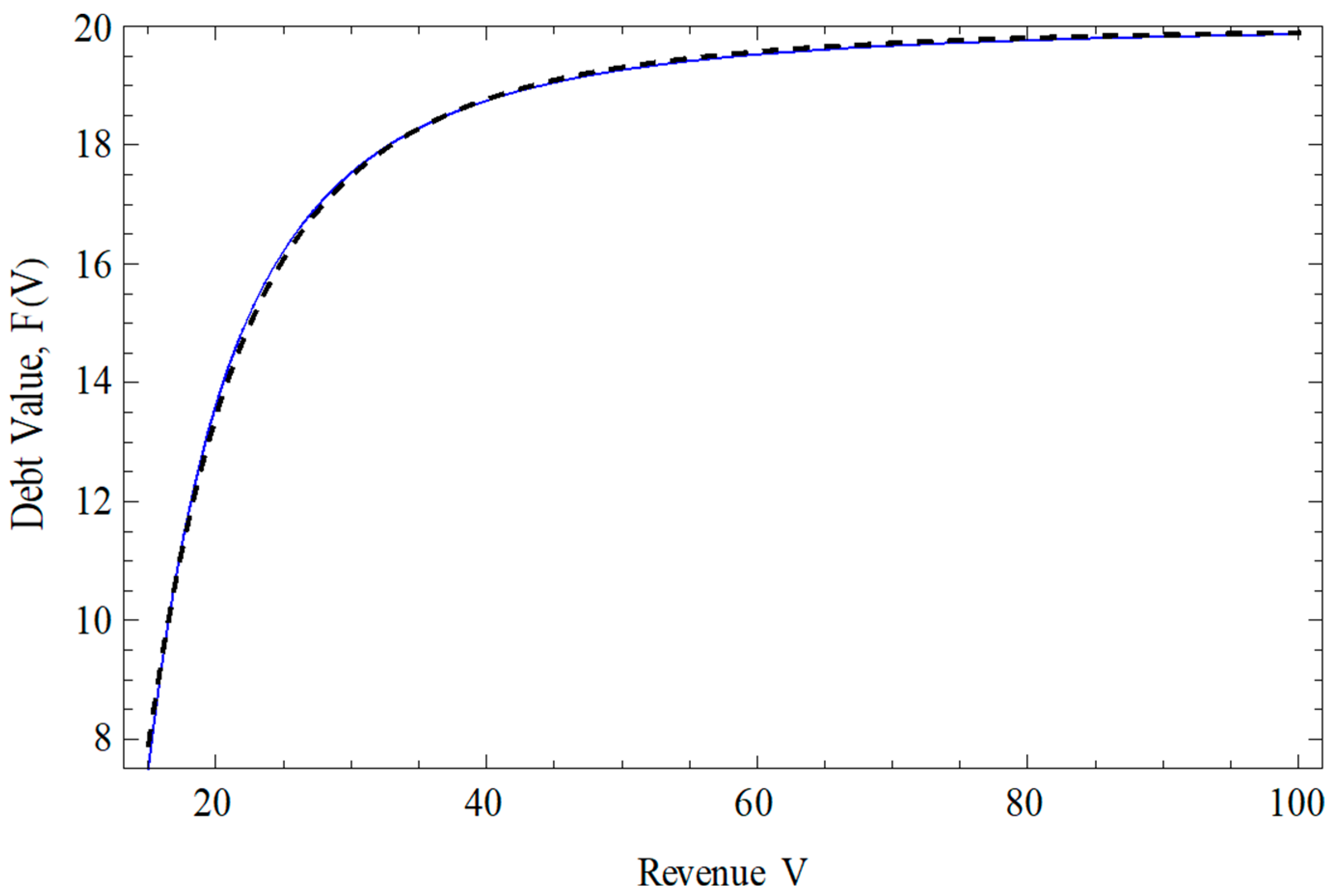
Figure 1. Comparison of Equation (24) (solid line) and the result of the numerical computation (dashed line).
Jrfm 18 00302 g001
Figure 2. Comparison of B F ( V ) between the models with the feedback of sovereign-debt credit to the country GDP (solid line) and without the feedback (dashed line).
Jrfm 18 00302 g002
Figure 3. Comparison of the sovereign debt value F(V) between the models with the feedback of the sovereign-debt credit to the country GDP (solid line) and without the feedback (dashed line).
Jrfm 18 00302 g003
Figure 4. Comparison of r S V between the models with the feedback of the sovereign-debt credit to the state GDP (solid line) and without the feedback (dashed line).
Jrfm 18 00302 g004
Figure 5. Comparison of σ F ( V ) between the models with the feedback of sovereign-debt credit to the state GDP (solid line) and without the feedback (dashed line).
Jrfm 18 00302 g005
Figure 6. Country debt default, economy, public finance, politics, and social sector (feedback effects).
Jrfm 18 00302 g006
Figure 7. Estimated path diagram of sovereign debt defaults (standardized coefficients).
Jrfm 18 00302 g007
Table 1. Definitions of the parameters and values used in the numerical simulations.
Panel A. Parameter values used in numerical simulationsPanel B. Definitions of parameters and variables in the search-based model
ParameterValueB—default boundary; C—annual coupon payment; q—asset position of agents; r—risk-free interest rate; X—parameter defined in Equation (22); Y—parameter defined in Equation (15); Z—parameter defined in Equation (A4); γ—recovery rate of debt; µ—growth rate of a country’s economy, denominated by the domestic currency; σ—GDP volatility
B15
C1
r5%
a ϵ 10 5
x 0.2
γ 0.5
μ 0.15
σ 0.3
Table 2. Comparative statics of domestic debt.
B F n γ F n C F n r F n Z F n r Z μ Z σ Z 1 B V B Z B ( Z + 1 ) γ C r Z B V B Z > 0 1 r 1 V B Z > 0 C r 2 1 V B Z < 0 V B Z C r B γ l n V B > 0 2 σ ( σ 2 μ ) 2 + 8 r > 0 4 μ 2 σ σ ( σ 2 μ ) 2 + 8 r + 1 σ > 0 μ 2 μ + σ ( σ 2 μ ) 2 + 8 r 4 r σ 2 ( σ 2 μ ) 2 + 8 r < 0
Table 3. Comparative statics of foreign debt.
B F 0 1 B V B Y B ( Y + 1 ) γ C r Y + r ( X Y ) B ϵ X
γ F 0 B V B Y > 0
C F 0 1 r 1 V B Y > 0
r F 0 C r 2 1 V B Y < 0
X F 0 B ϵ X V B Y l n B ϵ V B X l n V ϵ < 0
Y F 0 V B Y B ϵ X B γ + C r l n V B > 0
r X 2 r σ 3 / 2 σ + 8 r > 0
r Y 0
μ Y 2 σ 2 > 0
σ X 2 r σ 3 / 2 σ + 8 r < 0
σ Y 4 μ σ 2 < 0
Table 4. Description of variables.
VariableDescription
def_d_lgdefaulted debt level (logged)
ECONlatent variable—economy
gdpg_llagged GDP growth rate
infinflation
gfc_grgross fixed capital formation growth rate
ex_gdpexports/GDP
fdi_gdpFDI/GDP
cgd_gdpcentral government debt/GDP
ex_crisexchange rate crisis (local currency depreciating more than 15% against the USD)
FINANClatent variable—public finances
sd_tdeb short-term debt as a percentage of total public debt
sd_resshort-term debt as a percentage of reserves
res_debreserves as a percentage of total debt
imp_gdpImports-to-GDP ratio
rintrreal interest rate
ds_gdpdebt service as a percentage of GDP
trip_crtriple crisis, comprising banking, currency, and sovereign debt
POLITIClatent variable—domestic political system functioning
f_ter dummy variable representing finite term in office (=1)
milt military expenditure as a % of GDP
y_of years since government in office
y_cur years left in the current term
SOClatent variable—social sector
ge_edu country’s expenditures on education as a percentage of GDP
ge_heal country’s expenditures on health as a percentage of GDP
mort_rmortality rate
pri_comp primary education competition rate
Observed variables
usirUS interest rate
lib_rLIBOR rate
eco_greconomic GDP growth rate
dh_md history of medium levels of debt defaults (USD 50 million—<USD 1 billion)
dh_mjd history of high levels of debt defaults (>=1 billion USD)
Table 5. Sovereign debt default: social sector investment and conditions and feedback effects.
Coeff.SEP > |z| Coeff.SEP > |z|
def_d_lg ECONO
ECONO0.0210.0100.032def_d_lg−0.1030.0190.000
FINANC−0.0110.0080.145POLITIC−0.0260.0510.606
POLITIC−0.0260.0070.000SOC0.4760.0210.000
SOC−0.0290.0070.000FINANC
usir−0.0240.0110.032def_d_lg−0.1660.0240.000
lib_r0.0120.0120.309POLITIC−0.0050.0330.871
eco_gr−0.0050.0050.388SOC0.4930.0280.000
dh_md0.6290.0090.000SOC
dh_mjd0.8930.0090.000POLITIC−0.1850.0190.000
_cons0.4160.0140.000POLITIC
def_d_lg0.0310.0180.083
Measurement estimates of the SEM model are not reported in the above table but are available upon request.
Disclaimer/Publisher’s Note: The statements, opinions and data contained in all publications are solely those of the individual author(s) and contributor(s) and not of MDPI and/or the editor(s). MDPI and/or the editor(s) disclaim responsibility for any injury to people or property resulting from any ideas, methods, instructions or products referred to in the content.