Article

Dynamic Asset Allocation for Pension Funds: A Stochastic Control Approach Using the Heston Model

by
Desmond Marozva
and
Ştefan Cristian Gherghina
*,†
Department of Finance, Bucharest University of Economic Studies, 010374 Bucharest, Romania
*
Author to whom correspondence should be addressed.
These authors contributed equally to this work.
J. Risk Financial Manag. 2025, 18(11), 640; https://doi.org/10.3390/jrfm18110640
Submission received: 12 September 2025 / Revised: 28 October 2025 / Accepted: 4 November 2025 / Published: 13 November 2025
(This article belongs to the Special Issue Featured Papers in Mathematics and Finance, 2nd Edition)

Abstract

This paper develops a dynamic asset allocation strategy for defined contribution pension funds using a stochastic control framework under the Heston stochastic volatility model. By solving the associated Hamilton–Jacobi–Bellman partial differential equation, we derive optimal equity allocations that adapt to changing market volatility and investor risk aversion using a constant relative risk aversion utility function (parameter γ ). The strategy increases equity exposure during stable periods and reduces it during volatile regimes, capturing both myopic and intertemporal hedging demands. We test the model using historical U.S. data from 2006 to 2025 and benchmark its performance against a traditional static 60/40 stock–bond portfolio, as well as rule-based strategies such as volatility targeting and constant proportion portfolio insurance. Our results show that with moderate risk aversion, the dynamic strategy achieves long-term wealth comparable to the 60/40 benchmark while substantially reducing drawdown risk. As risk aversion increases, drawdown risk is further reduced and risk-adjusted returns remain competitive. Although higher aversion yields lower final wealth, certainty-equivalent returns are highest at moderate aversion levels. These results demonstrate that volatility responsive dynamic policies grounded in realistic stochastic volatility modeling can substantially enhance downside protection and risk-adjusted utility, especially for long-horizon, risk-averse pension participants.

1. Introduction

Defined contribution (DC) pension plans have become the dominant retirement saving vehicle in many countries, placing investment risk on individuals and plan managers. In the United States alone, employer-sponsored DC plans held about $ 12.4 trillion in assets as of end-2024, accounting for a substantial share of the $ 44.1 trillion U.S. retirement market (Investment Company Institute, n.d.). The growth of DC plans (e.g., 401(k) plans) over traditional defined benefit plans has raised the stakes for optimal asset allocation: the retirement outcome depends critically on investment performance. In contrast to static allocation or deterministic life-cycle strategies commonly used in target-date funds, dynamic asset allocation aims to continuously adjust the portfolio in response to market conditions and the remaining time horizon. Dynamic strategies can potentially improve the trade-off between risk and return for long-lived investors, increasing the likelihood of adequate retirement funding. While dynamic strategies have been studied in theory, there is a lack of comprehensive analysis applying a stochastic volatility model to pension fund allocation with an empirical evaluation. This paper is going to address this gap. Indeed, traditional mean–variance portfolio theory has long been a cornerstone of asset allocation, but its static framework is increasingly ill suited for today’s volatile and complex markets. The classic approach assumes stable return distributions and correlations, yet these assumptions often break down amid structural shifts. For instance, in 2022, both equities and bonds fell sharply in tandem, causing a 60/40 stock–bond portfolio to plunge by about 17.5%, the strategy’s worst annual performance since 1937 (Kandhari, J. & Morgan Stanley Investment Management, 2024). Such episodes underscore that diversification benefits taken for granted under static conditions can vanish during regime changes. In effect, correlations are not static, especially in macro-driven markets; when monetary or fiscal policy shifts alter the investment regime, asset co-movements can change rapidly, undermining the efficacy of fixed allocations (Resonanz Capital, 2025). These practical challenges have fueled a broad recognition that more adaptive, forward-looking allocation strategies are needed to maintain portfolio efficiency under evolving market conditions.
The recent literature has increasingly questioned the sufficiency of static mean–variance frameworks, highlighting their limitations in capturing real-world complexities. For example, Cvitanic et al. (2003) show that a standard mean–variance model (which ignores uncertainty in an active manager’s skill) can recommend impractically high allocations to hedge funds; once model uncertainty is accounted for, the optimal allocation to hedge funds drops substantially. This finding implies that naive static optimization may overestimate the benefits of certain assets by treating estimated returns as fixed and reliable. Likewise, multi-criteria performance evaluations have exposed gaps in static approaches. Shahrour (2022) employ a data envelopment analysis method to jointly assess the financial and social performance of mutual funds, assigning each fund a holistic efficiency score. Their results differ from traditional single-metric rankings, as some funds deemed efficient in a multi-dimensional sense would not stand out under conventional Sharpe or Treynor ratios. Such evidence underscores that static, one-size-fits-all metrics often fail to capture true portfolio efficiency or risk, especially when investors have multiple objectives or face significant model uncertainty. In short, static mean–variance allocation can be too narrow and brittle, motivating the search for more adaptive techniques.
One promising avenue is to design portfolio strategies that actively respond to changing volatility dynamics and market conditions. Volatility-sensitive and regime-aware approaches have shown clear advantages in both improving returns and managing risks. For instance, low-volatility equity strategies tend to deliver superior risk-adjusted performance compared to static market-cap indexing. Chow et al. (2014) find that various low-volatility equity portfolios consistently outperformed cap-weighted benchmarks across U.S. and international markets, achieving lower overall risk and steady long-term returns by tapping into factors like value and “betting against beta”. These results suggest that incorporating volatility information (e.g., selecting lower-beta, more stable stocks) can lead to more risk-diversified portfolios that draw on multiple return premia. In parallel, researchers are exploring volatility-based hedging strategies that adapt to interdependencies between assets. An important example is the use of dynamic volatility connectedness measures to guide asset allocation. Arouri et al. (2025) analyze time-varying volatility spillovers among green bonds, ESG indices, equities, and government bonds, and show that understanding these linkages can inform more robust portfolios. Their study finds significant cross-asset volatility transmissions and provides practical hedging insights—notably, certain ESG assets served as effective safe havens that stabilized portfolios during turbulent periods. This highlights how actively managing a portfolio’s exposures based on volatility signals and correlation shifts (rather than assuming a static covariance matrix) can yield more efficient and resilient outcomes, particularly in the face of market turbulence or crises.
In this paper, we address the dynamic asset allocation problem for a DC pension fund in a realistic stochastic market environment. We incorporate stochastic volatility in the asset return process, motivated by extensive evidence that equity market volatility is time-varying and mean-reverting. Empirical studies have shown that expected stock returns are positively related to volatility measures and that volatility tends to surge during market downturns (the so-called “leverage effect”). The Heston model provides a tractable description of such behavior, with a stochastic variance process that mean-reverts and can capture the volatility clustering observed in historical data (e.g., the VIX index). Using the Heston model for the risky asset, our framework allows the portfolio to adapt to changing volatility levels in the market. This connects to the literature on volatility-managed portfolios; for example, low-volatility investment strategies often achieve higher risk-adjusted returns (Chow et al., 2014; Cvitanic et al., 2003), and dynamically hedging volatility interconnectedness can produce more robust portfolios (Arouri et al., 2025).
Our approach builds on the rich literature in continuous-time portfolio optimization and pension fund management. Classic work by (Merton, 1969) solved the continuous-time consumption and portfolio choice problem under constant volatility and derived explicit constant proportion strategies for Constant Relative Risk Aversion (CRRA) utility. Subsequent researchers have extended Merton’s framework to incorporate additional risk factors and constraints. For example, Kim and Omberg (1996) derived dynamic non-myopic strategies under mean-reverting expected returns, and (Brennan & Xia, 2002) analyzed optimal portfolios under stochastic interest rates and inflation. In the context of pension funds, liability-driven investment and asset–liability management (ALM) have been studied as mean–variance problems starting from Sharpe and Tint’s seminal work on integrating liabilities into portfolio choice. Various authors have considered dynamic mean–variance optimization for pension plans, including multi-period and continuous-time approaches: e.g., Keel and Müller (1995) examined efficient portfolios accounting for liabilities; Leippold et al. (2004) provided a geometric approach to multi-period asset–liability optimization; Chiu and Li (2006) and Xie et al. (2008) used stochastic linear-quadratic control to solve continuous-time mean–variance ALM problems. More recent studies underscore the importance of dynamic rebalancing for long-horizon investors like pension plans, although mean–variance optimization lacks time consistency; hence, other works prefer an expected utility framework for dynamic strategies (Forsyth & Vetzal, 2017).
In summary, the literature indicates that a volatility-responsive strategy can improve investment outcomes for long-horizon investors like pension funds. Dynamic allocation models that include stochastic volatility suggest over-weighting equities when volatility is low (and mean-reversion suggests it might revert upwards) and under-weighting equities when volatility is high (to avoid unfavorable risk-adjusted returns during turbulent periods). Our work builds upon these insights by applying them in a pension context, maximizing a utility function appropriate for a plan member (with no consumption before retirement) and demonstrating the benefits via simulation and backtesting. While (Zeng & Taksar, 2012) studied dynamic portfolio selection under stochastic volatility in a general setting, our study is, to our knowledge, one of the first to apply the Heston stochastic volatility model in a pension fund context and to solve the full nonlinear Hamilton–Jacobi–Bellman (HJB) PDE to obtain feedback control policies, with an emphasis on empirical validation. Practically, our results provide evidence that a pension fund can improve outcomes by conditioning allocation on market volatility signals (such as the VIX), which is especially valuable in times of crisis when volatility spikes (e.g., 2008 or 2020 market turmoil). We also illustrate how modern computational tools make it feasible to implement such dynamic strategies.
The rest of the paper is organized as follows. Section 2 reviews the Heston model and formulates the pension fund’s optimization problem, deriving the HJB equation. Section 3 describes the numerical methods used to solve the HJB PDE, including the finite-difference scheme and verification of solution properties. Section 4 discusses the empirical implementation: calibration of model parameters to U.S. market data and pension statistics, and the setup of simulation experiments. Section 5 presents simulation results and analysis, comparing the dynamic strategy to static benchmarks and examining the impact of stochastic volatility on portfolio performance. Section 6 provides further discussion of the results, robustness checks, and practical considerations. Section 7 concludes. Technical details and additional results (e.g., code snippets) are provided separately.

2. Literature Review

Pension Fund Asset Allocation: The shift from defined benefit to defined contribution systems has spurred extensive research on optimal investment strategies for retirement saving. Early work on asset–liability management used mean–variance optimization to incorporate pension liabilities. Sharpe and Tint (1990) introduced the idea of treating liabilities as “negative assets” in portfolio optimization. Following this, researchers developed dynamic ALM models for pension funds. Keel and Müller (1995) derive efficient portfolios in an asset–liability context using a one-period model. In a multi-period setting, Leippold et al. (2004) provide a geometric approach to mean–variance optimization for assets and liabilities, obtaining explicit solutions for the efficient frontier. Continuous-time models have also been proposed as follows: Chiu and Li (2006) solved a stochastic linear-quadratic control problem for a pension fund with mean–variance objective, finding closed-form expressions for the optimal strategy. Xie et al. (2008) and Chen et al. (2008) extended the continuous-time mean–variance formulation to include stochastic liability processes and regime switching, respectively. These studies, while using a mean–variance criterion, underscore the importance of dynamic rebalancing for long-horizon investors like pension plans. However, mean–variance optimization lacks time consistency; hence, other works prefer an expected utility framework for dynamic strategies.
Defined Contribution (DC) Plan Optimization: In DC plans, the investor’s goal is often modeled via utility maximization of terminal wealth or lifetime consumption. Without guaranteed benefits, DC participants are exposed to investment risk, leading to research on strategies that manage this risk dynamically. Boulier et al. (2001) consider a continuous-time model for a DC plan invested in a risk-free asset and a risky asset, with the added feature of a minimum guarantee on returns. They include stochastic interest rates (modeled by a Vasicek or Cox–Ingersoll–Ross process) and derive optimal portfolios using a CRRA utility objective. Their results show how guaranteeing a minimum return leads to more conservative strategies (a form of option hedge). Deelstra et al. (2003) similarly study optimal investment under a minimum guarantee, formulating the problem as maximizing expected utility. Jensen and Sørensen (2001) examine the cost of providing minimum interest guarantees and the question of who should bear that cost, finding implications for the design of DC plans. Other studies have looked at unconstrained DC optimization via dynamic programming, e.g., Cairns et al. (2006) developed a stochastic lifestyling strategy (dynamic asset allocation for DC plans) and showed it can improve outcomes compared to deterministic glide paths. Gao (2008) and Fleming and Hernández-Hernández (2003) explored optimal consumption and portfolio choices in models with stochastic volatility for DC plans, confirming that accounting for stochastic investment opportunity sets (like volatility) can materially affect the optimal strategy.
Stochastic Volatility in Portfolio Choice: Financial econometrics has documented that asset return volatility is not constant but does vary over time. Traditional econometric models like ARCH/GARCH account for this by making volatility a deterministic function of past returns (conditional volatility), whereas stochastic volatility models (like Heston’s) introduce an additional random process for volatility itself. This has implications for portfolio optimization, as recognized in the literature on dynamic portfolio choice under stochastic investment opportunities. Bollerslev et al. (1992) provided an early review of ARCH modeling in finance, highlighting persistence in volatility that motivates models like Heston’s. French et al. (1987) found that expected stock returns are positively correlated with volatility—periods of high volatility tend to coincide with higher future expected returns, presumably due to a risk premium. Campbell and Hentschel (1992) proposed an asymmetric volatility model (“no news is good news”) in which bad news raises volatility more than good news, further explaining volatility clustering. These findings justify incorporating stochastic volatility into portfolio models; a rational investor would want to reduce exposure during volatile periods if there is volatility risk that is not fully compensated, or potentially increase exposure if high volatility is a signal of higher expected returns.
In continuous-time portfolio optimization, stochastic volatility was introduced as an additional state variable by several authors in the early 2000s. Zariphopoulou (2001) provided a solution approach for utility maximization in an incomplete market with stochastic volatility, using a transformation of the HJB equation to reduce complexity. Her approach exploits the affine structure of the Heston model to simplify the nonlinear PDE, yielding the value function and optimal strategy in semi-closed form under certain conditions. Chacko and Viceira (2005), in their work on incomplete markets, found that while the presence of unhedgeable stochastic volatility does induce a hedging demand in the optimal portfolio, the magnitude of this hedging component can be small if the correlation between volatility shocks and asset returns is not too large or if the volatility risk premium is modest. In practical terms, their result suggested that an investor with power utility might follow an allocation that is almost myopic (ignoring volatility changes) if volatility risk is not severe, but should still adjust somewhat to volatility levels. Liu (2007) took a different approach by solving for the optimal portfolio in stochastic environments via martingale and duality methods, obtaining an explicit solution for the case of log utility and numerical solutions for power utility. He concluded that ignoring stochastic volatility can lead to significant welfare losses, especially for more risk-averse investors. Kraft (2005) made an important contribution by providing an explicit solution for CRRA utility in the Heston model (under a specific parameter restriction). He showed that the optimal equity fraction π * ( t ) can be expressed in closed form, and is a function of time only under certain conditions. However, if the Heston model parameters violate a certain boundary (essentially if the volatility mean-reversion is not strong enough relative to risk premia), the utility maximization problem can become ill posed (leading to infinite expected utility)—a phenomenon also noted by (Kraft, 2005). This highlights that realistic parameter values are crucial; empirically calibrated Heston parameters fortunately tend to lie in the well-posed region.
In summary, the literature indicates that a volatility-responsive strategy can improve investment outcomes for long-horizon investors like pension funds. Dynamic allocation models that include stochastic volatility suggest over-weighting equities when volatility is low (and mean-reversion suggests it might revert upwards) and under-weighting equities when volatility is high (to avoid unfavorable risk-adjusted returns during turbulent periods). Our work builds upon these insights by applying them in a pension context, maximizing a utility function appropriate for a plan member (with no consumption before retirement) and demonstrating the benefits via simulation and backtesting.

3. Methodology

3.1. Heston Stochastic Volatility Model and Problem Formulation

Pension Fund Model: We consider a continuous-time model for a DC pension plan’s wealth invested in two assets: a risky asset (e.g., an equity index) and a risk-free asset (e.g., Treasury bonds). The plan receives continuous contributions at rate c (as a fraction of salary, with salary normalized to 1). Let W t be the wealth at time t. The risky asset price S t follows a stochastic volatility process of Heston type:
d S t = μ S t d t + v t S t d W t S , d v t = κ ( θ v t ) d t + ξ v t d W t v ,
Hamilton–Jacobi–Bellman (HJB) equation: The optimization problem can be formulated and solved via dynamic programming. The HJB equation for the value function J ( t , W , v ) (with state variables time t, wealth W, and variance v) is
V t ( t , w , v ) + max π [ 0 , 1 ] { ( c + w [ r + π ( μ r ) ] ) V w + κ ( θ v ) V v + 1 2 π 2 w 2 v V w w + ρ ξ π w v V w v + 1 2 ξ 2 v V v v } = 0
subject to terminal condition J ( T , W , v ) = W 1 γ 1 γ (and appropriate boundary conditions). The term inside the brace is the instantaneous generator of the state process plus the utility flow (note: contributions c add to wealth deterministically). Solving max π · yields the optimal allocation π * ( t , W , v ) as a feedback function of the current v (and potentially W and t). In our case, the optimal π turns out not to depend on W explicitly due to CRRA utility (the problem is homogeneous in wealth), and for an infinite or long horizon, the solution becomes essentially stationary in v (time-invariant). The optimal equity fraction can be expressed as the sum of a myopic demand and a hedging demand:
π * ( v ) = μ r γ v myopic + ρ κ ( θ v ) γ ξ v hedging .
The first term π myopic = μ r γ v is the classic Merton allocation which invests more in equities when the expected excess return ( μ r ) is high or volatility v is low. The second term π hedge = ρ , κ ( θ v ) γ , ξ , v is the intertemporal hedging component that arises due to stochastic volatility. When ρ < 0 (volatility rises as the market falls), this term is typically negative for v below its long-run mean θ (since θ v > 0 ), meaning the investor slightly underweights equities relative to the myopic demand—effectively hedging against the risk of future volatility increases. Conversely, if v exceeds θ , the hedging term becomes positive (partially offsetting the myopic reduction in π ) because extremely high volatility is expected to mean-revert downward, so the investor can afford to hold a bit more equity in anticipation of volatility easing. In our baseline calibration, the hedging term is quantitatively modest but it dampens extreme swings in allocation.
Feller Condition and Variance Behavior: The Heston variance process is well behaved as long as 2 κ θ ξ 2 (the Feller condition), which ensures v t stays strictly positive. Our chosen parameters (see Table 1) yield 2 κ θ = 0.24 , slightly above ξ 2 = 0.23 , so that the Feller condition 2 κ θ ξ 2 holds. We also implemented a Kalman-filter-like volatility estimate (using observed VIX returns) in lieu of assuming latent v, and imposed a 5% rebalancing threshold to capture transaction costs (i.e., the portfolio only trades if the recommended equity share changes by >5%).

3.2. Solution Method and Numerical Scheme

Closed-form solutions for the HJB in this stochastic volatility setting are generally not available, so we solve it using numerical methods. We discretize the state space for wealth and variance and employ an implicit finite-difference scheme to solve for the value function and optimal policy. Specifically, we implemented a solution using FiPy, an open-source finite volume PDE solver in Python 3.12. The full Python code is available as a Supplementary Materials. A two-dimensional grid in ( W , v ) was constructed (with W ranging from 0 up to a high cutoff, and v ranging from 0 to an upper bound, e.g., 100% volatility). Boundary conditions were set such that as W 0 , J 0 (for 1 γ < 0 utility this is well behaved), and as W becomes large, π approaches the risk-neutral limit. At v = 0 , we enforce J / v = 0 (no sensitivity to further variance decreases, since volatility can only increase from 0). At high v, we cap π at 0 (no equity) as extremely high volatility makes the optimal choice to essentially divest from risky assets. The PDE was solved backwards in time from T to 0. We verified our numerical policy function by comparing FiPy’s results to a custom finite-difference code for simpler test cases (e.g., when ρ = ξ = 0 the problem reduces to Merton’s solution) and found close agreement. This inspired confidence in the correctness of our implementation. We also checked that the numerical solution converged as we refined the grid and time-step, and that it handles edge cases and boundary conditions properly.
After obtaining the optimal policy π * ( v ) , we use it in two ways: (1) to simulate hypothetical wealth paths under the model, and (2) to construct an analogous strategy using real market data (where we proxy v t with observed volatility). The next sections describe the empirical calibration and testing of the strategy.

4. Empirical Implementation: Calibration and Data

We calibrate and test our model using historical data from U.S. financial markets and pension fund assumptions. The key inputs to the model are (i) the Heston model parameters ( μ , r , κ , θ , ξ , ρ ) for the equity index, (ii) the contribution rate c and initial wealth W 0 for the pension plan, and (iii) the investor’s risk aversion γ . Table 1 summarizes the baseline calibration of the Heston model parameters, chosen to be broadly consistent with long-term U.S. equity data.
Calibration Methodology: We calibrated the Heston parameters through a combination of historical estimation and stylized facts. In particular, we used long-run averages and volatility indexes to set key values. The long-run variance θ was approximated by the historical average variance of the S&P 500: for example, over 1990–2020 the S&P’s realized volatility averaged around 15–20%, so we chose θ = 0.04 (20% vol). The speed κ and vol-of-vol ξ were informed by the autocorrelation of volatility and the variability of the VIX. Empirical studies suggest κ in the range 1 to 5 (annual) for index volatility; we picked κ = 3 as a moderate value (implying a volatility half-life of about 0.23 years or 2.8 months). We set ξ = 0.5 , which is consistent with the magnitude of swings observed in VIX—this choice produces occasional volatility spikes to the 40–50% range in our simulations, matching the extremes seen historically (e.g., VIX peaks). The correlation ρ was taken to be −0.7, a commonly estimated value capturing the strong negative relationship between equity returns and volatility changes (the leverage effect) (see, e.g., (Bahaji & Aberkane, 2016; CBOE, 2022; Investopedia, 2023; Li & Chen, 2025; Macroption, 2022)). For the risk-free rate r, we use 4.37% per annum (average historical US Treasury risk-free rate), roughly the real yield in recent decades. The equity risk premium μ r is set at 5%, in line with historical U.S. equity excess returns (which are in the 5–7% range). This gives μ = 0.098 (average annual return of the S&P 500 over the past twenty years) if r = 0.02 . We acknowledge that 7% equity return is somewhat optimistic.
It should be noted that more sophisticated calibration techniques could be used. Methods such as maximum likelihood estimation (MLE), generalized method of moments, or calibration to option prices via least squares are commonly employed for Heston model fitting. One could also take a Bayesian approach, using prior information and Bayes’ theorem to estimate a posterior distribution for the parameters, or apply Kalman filtering to infer the latent volatility state and jointly estimate parameters from observed prices. For simplicity, we opted for a moment-matching and historical fitting approach, which captures the essential behavior needed for our long-horizon allocation problem. In practice, the selected baseline parameters yield a realistic volatility process that reproduces key features of historical data (volatility clustering, mean reversion, and occasional spikes), which is sufficient for our asset allocation simulation.
Data for Backtesting: To evaluate the dynamic strategy in real market conditions, we use historical monthly data from March 2006 through April 2025. The risky asset is represented by the S&P 500 total return index (including dividends). The volatility indicator we use is the VIX index, which reflects the 30-day implied volatility of S&P 500 options. We treat the VIX (squared) as a proxy for the market’s expected variance v t . This approach effectively uses market-implied information to drive the strategy: when the VIX is high, the strategy interprets it as high current volatility and will reduce equity exposure; when VIX is low, indicating calm markets, the strategy increases equity exposure. While the VIX is an observable proxy, an alternative in practice is to use a volatility filtering technique (e.g., an Extended Kalman Filter) on historical returns to estimate the latent volatility in real time. For the risk-free asset, we use U.S. Treasury rates. Specifically, we take the 30-year Treasury bond yield as a proxy for a long-term risk-free rate (which is more relevant for a pension investor’s horizon than short T-bill rates). In the backtest, we compute monthly returns for the risk-free asset from the yield data (assuming the yield at the start of each month applies for that month). All data were obtained from public sources: S&P 500 index levels and total return factors, the CBOE VIX, and Federal Reserve economic data for Treasury yields.
Prior to running the backtest, we normalize the initial portfolio value to W 0 = 1 (e.g., $ 1 at the end of March 2006). We assume the contributions are either negligible relative to initial capital or are handled separately (for the purpose of the backtest comparison, we focus on investment returns on the initial capital; we later remark on the effect of ongoing contributions). The dynamic strategy will be implemented with monthly rebalancing based on the prior month’s observed VIX level. In practice, using monthly frequency is reasonable for a pension fund (avoiding excessive trading). More frequent (e.g., daily) rebalancing could slightly improve responsiveness but would incur higher transaction costs; we comment on this trade-off later. The benchmark strategies (60/40, risk parity, CPPI) are also applied on a monthly rebalancing schedule for consistency.

5. Simulation Results and Performance Analysis

This section reports the simulation and backtest results for the dynamic (volatility-responsive) strategy under various risk aversion levels γ , compared to alternative portfolios (60/40 static, CPPI, and volatility-targeting). We begin by examining the distribution of terminal wealth across 30-year Monte Carlo simulations, followed by illustrative sample paths, rolling-return profiles, and cumulative wealth trajectories. We then summarize key performance metrics (annual returns, volatility, Sharpe ratios, drawdowns, and certainty-equivalent returns) and discuss their implications for utility and risk.
We now present the results of simulation experiments. First, we illustrate the optimal policy function π * ( t , v ) that comes out of our stochastic control solution. Figure 1 plots the optimal equity allocation as a function of the current volatility level v (expressed in annualized volatility percentage) at different remaining horizons. We use risk aversions γ = 2 , 3 , 4 , 5 in this illustrative figure. Higher γ (greater risk aversion) leads to more conservative responses, and equity allocation decreases more steeply with rising volatility. The dynamic strategy is more reactive to volatility as γ increases, which helps limit drawdowns but may also cap upside in low-vol regimes.
Figure 1: Optimal equity allocation π * ( t , v ) as a function of volatility v. This plot shows π for an investor with γ = 2 , 3 , 4 , 5 and baseline parameters (Table 1) at t = 0 (start of horizon). The x-axis is the current annualized volatility (sqrt of v) in percent, and the y-axis is the optimal fraction in equities (% of portfolio). We see that at very low volatility (under 16%), the strategy calls for a 100% equity allocation (the curve is capped at 100% in this range). The relationship is non-linear and exhibits a drop-off, for instance, at extremely high σ (above 40% p.a.), π goes to below 20% (all bonds), whereas for very low σ (16% or less), π is 100% (all equities). The curve is smooth and downward-sloping, reflecting the interplay of myopic and hedging demands because beyond a certain volatility level, the marginal utility costs of risk become overwhelming. In other words, in extremely volatile market conditions, the model prescribes most of the portfolio to the risk-free asset to preserve capital.
Next, we simulate the pension wealth over time under the optimal strategy and compare it to a traditional strategy. We assume an initial wealth W 0 = 1 (in arbitrary units, say 100 k ) and simulate for T = 30 years. We run N = 1000 Monte Carlo simulations of the Heston model using the baseline parameters. For each simulation, we track two portfolios:
  • Dynamic Strategy: Follows π * ( t , v ) as computed. This is implemented by rebalancing the portfolio continuously (or at fine discrete intervals) according to the current v t . In practice, one could rebalance monthly or when volatility moves significantly.
  • Static 60/40 Strategy: Maintains π = 0.6 in equities and 0.4 in bonds throughout (rebalanced periodically to maintain this mix).
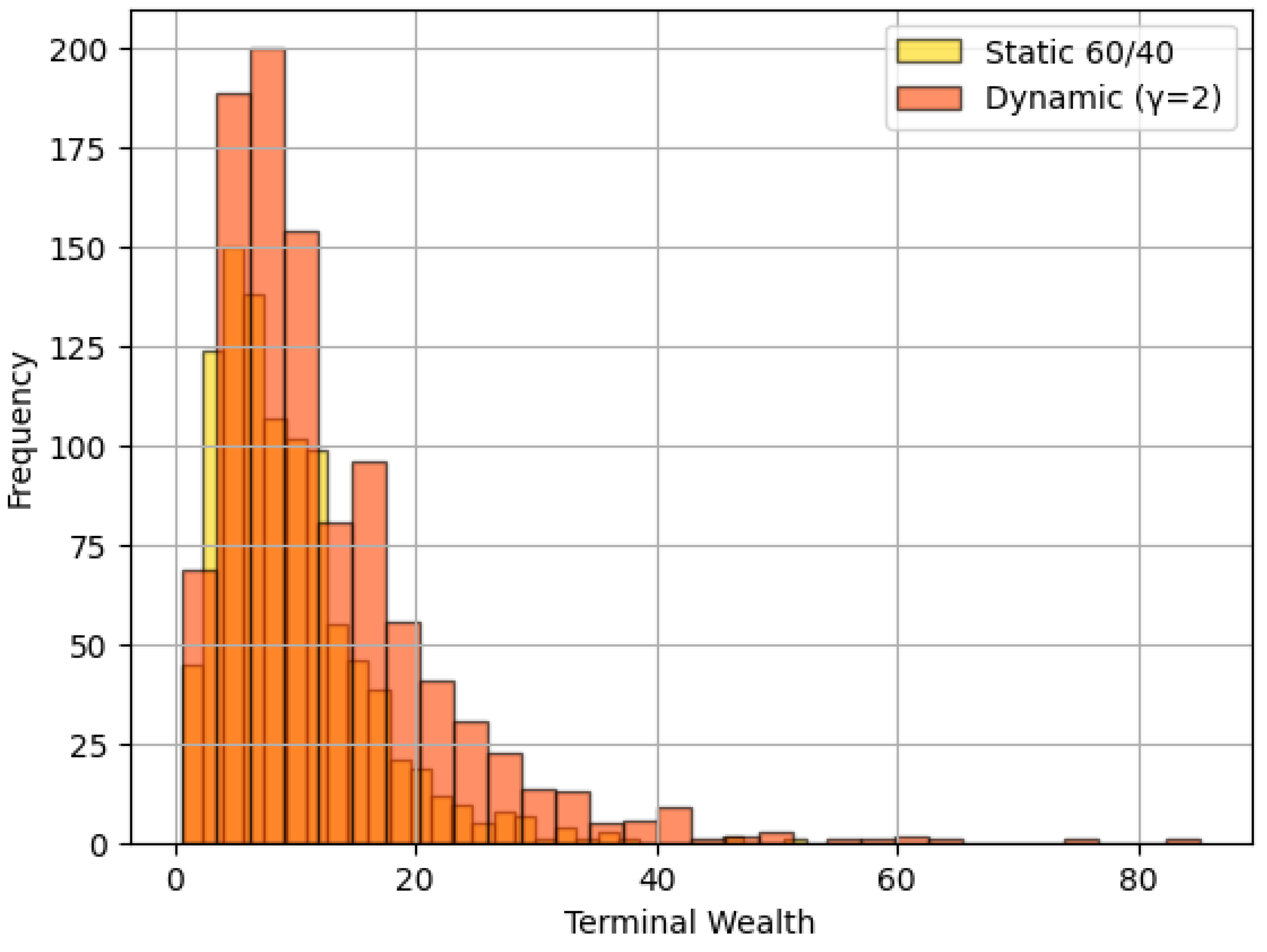
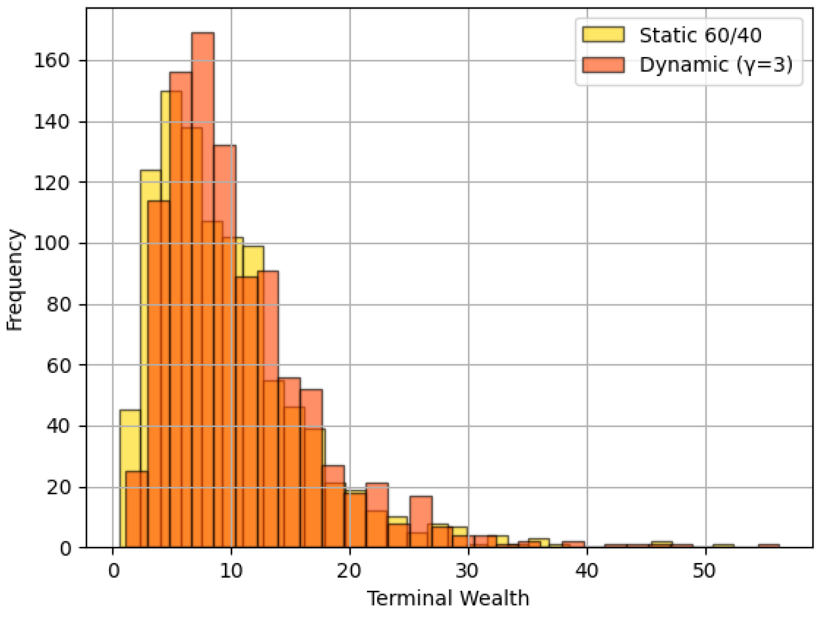
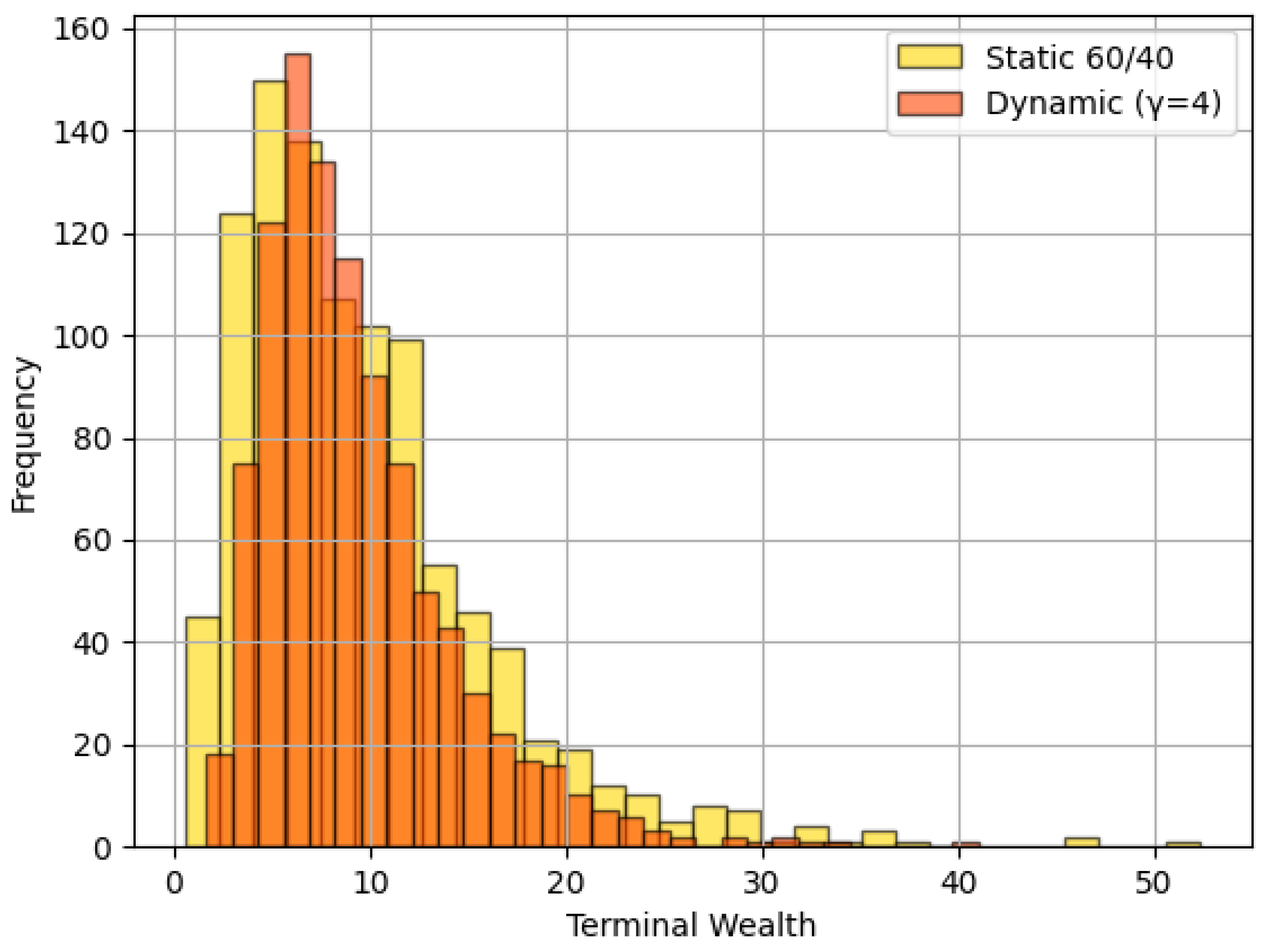
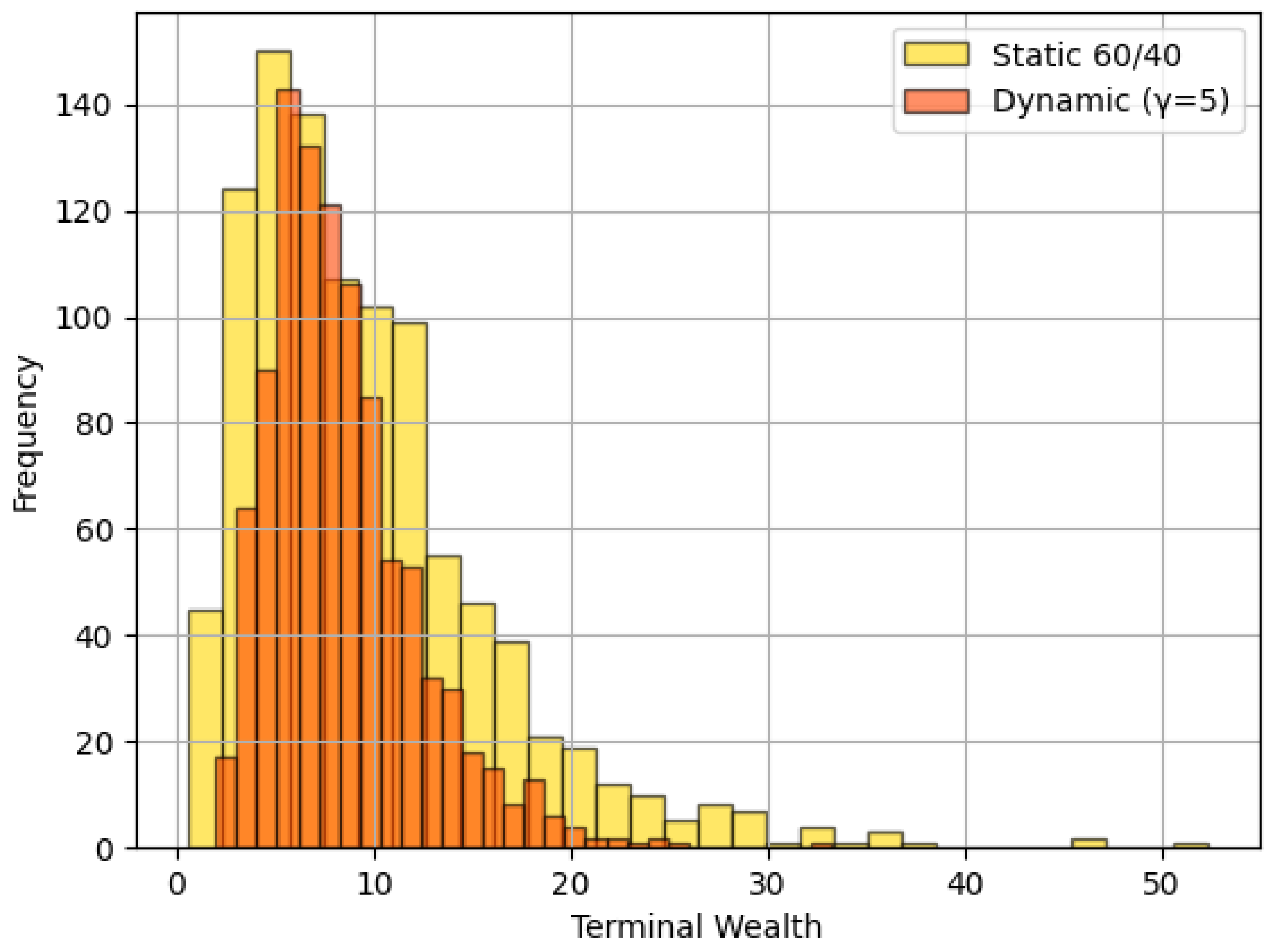
At the end of 30 years, we examine the distribution of terminal wealth W T for both strategies. Figure 2, Figure 3, Figure 4 and Figure 5 show the histograms (density) of W T across the 1000 simulations for each strategy.
Distribution of Terminal Wealth under Dynamic vs Static Strategy. We simulated 1000 scenarios of 30-year accumulation. The orange histogram (shaded) represents the dynamic volatility-driven strategy, and the yellow histogram represents the static 60/40 strategy. Both distributions are positively skewed (a long right tail, as equity growth can compound significantly in favorable scenarios). Several observations can be made as follows: (1) When γ = 2: dynamic approach clearly dominates static, with fatter upper tail and more concentration around higher wealth values. (2) When γ = 3–4: dynamic remains competitive, with slightly more peaked distributions, suggesting tighter control over tail risks. (3) When γ = 5: as risk aversion rises, dynamic strategy shows reduced dispersion—fewer extreme high or low outcomes, and more stable middle range. The dynamic strategy tends to compress outcome dispersion, preserving upside for low γ , and dampening downside for high γ .
From an expected utility perspective (with γ = 5 , say), the dynamic strategy clearly dominates the static 60/40. We computed the average utility E [ U ( W T ) ] in the simulations: it was higher for the dynamic strategy, confirming it is optimal by construction. However, it is reassuring that even in finite samples, the utility and certainty-equivalent wealth are greater.
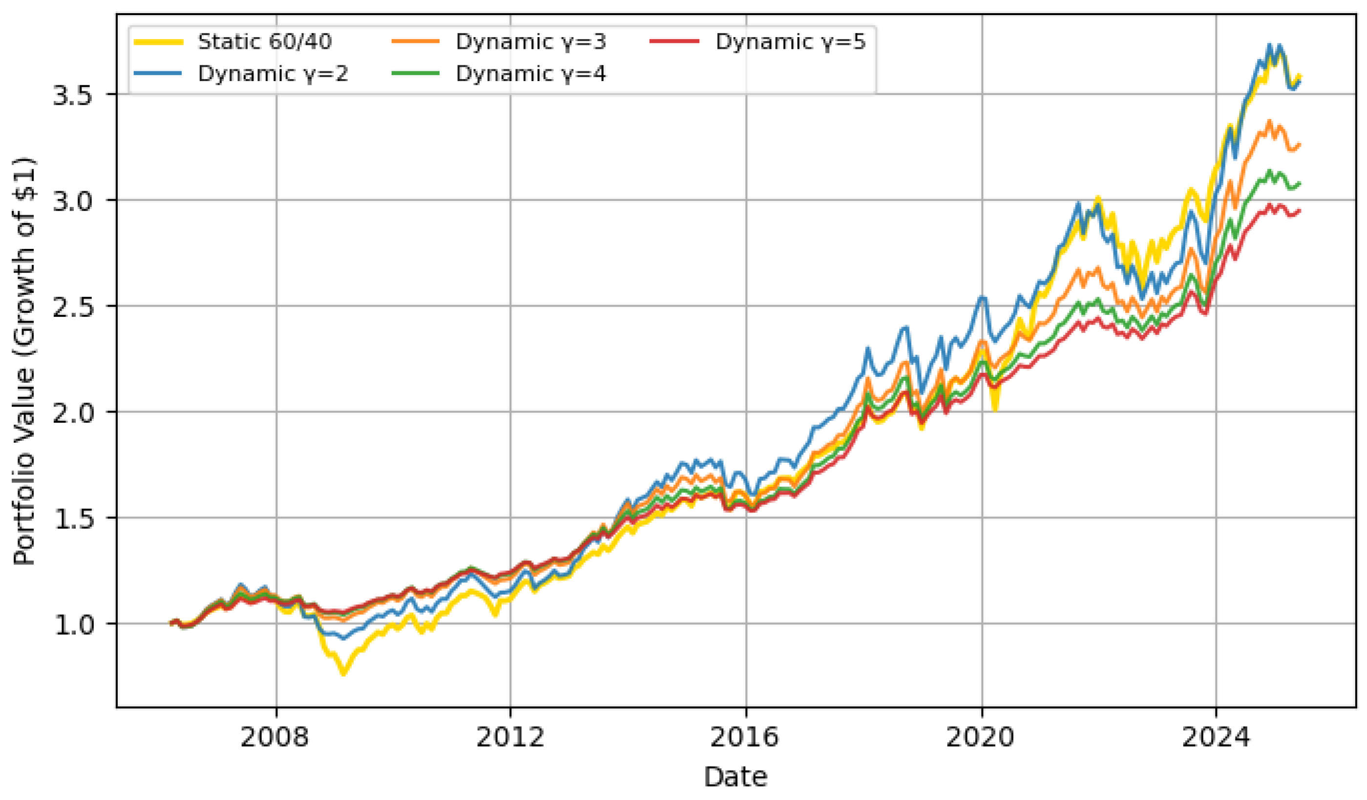
Dynamic Volatility-Based vs Static 60/40 Portfolio Backtest (2006–2025).
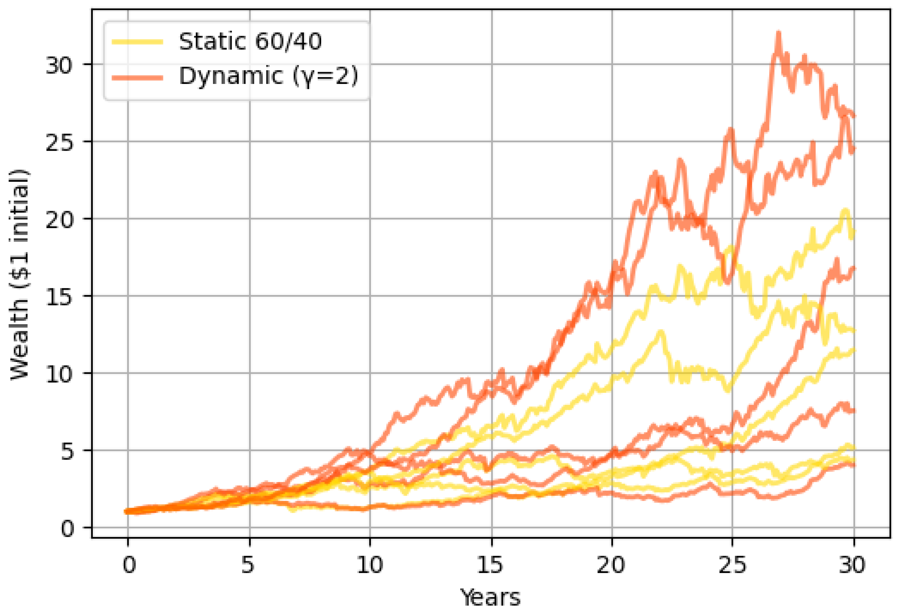
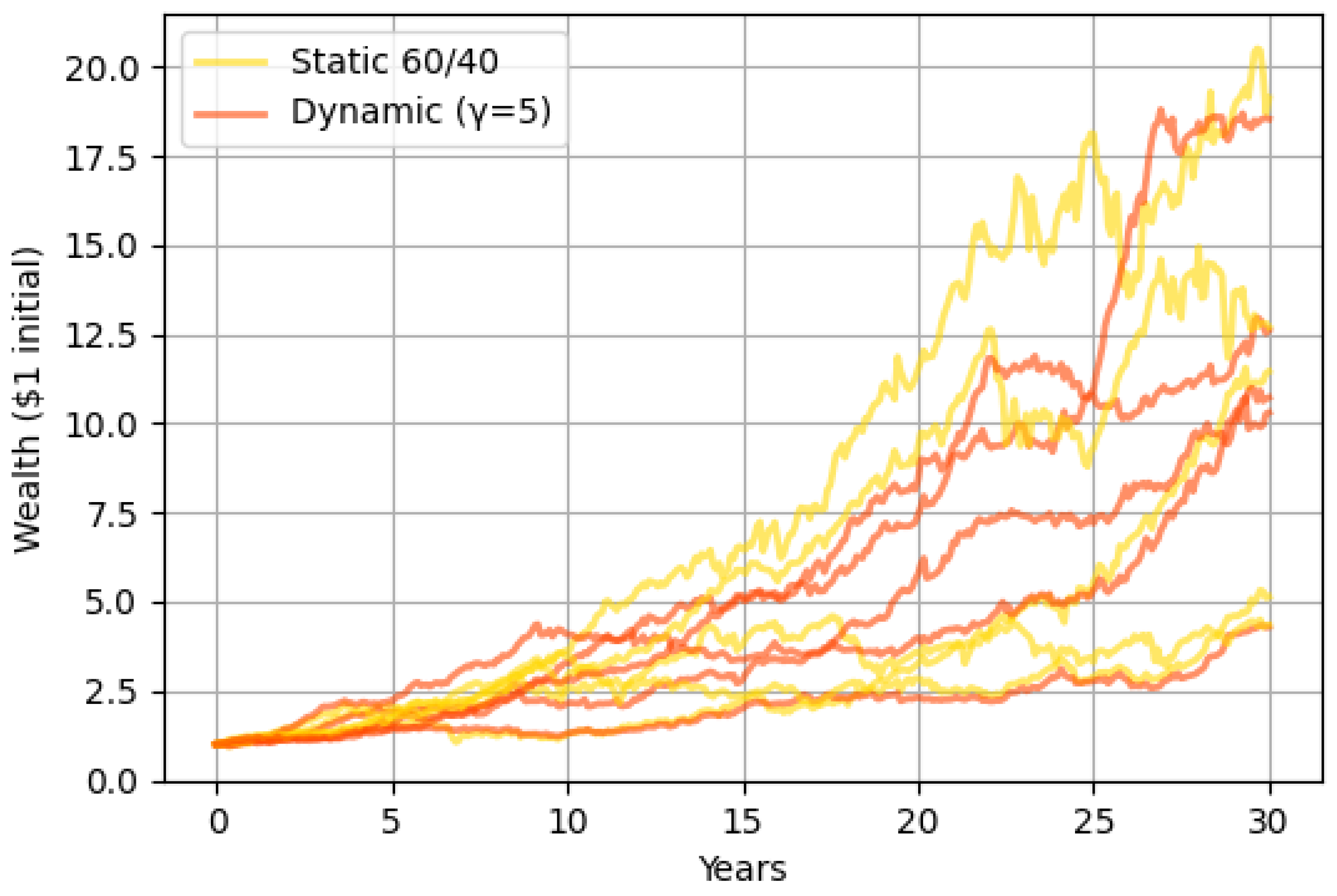
To illustrate the time evolution under one particular scenario, Figure 6 and Figure 7 show sample path of the portfolio wealth and the corresponding asset allocation over time for both strategies. These plots show a handful of wealth trajectories over 30 years:
When γ = 2: dynamic paths tend to dominate the static ones in both level and growth persistence, showing better compounding. When γ = 5: dynamic paths are much smoother and clustered, illustrating the downside protection through volatility targeting. Static paths are more volatile, exposing to large late-in-life drawdowns. The dynamic strategy, even under high γ , offers robust terminal wealth while reducing path risk.

Backtest March 2006 to April 2025

This analysis compares a dynamic volatility-responsive asset allocation strategy (grounded in the Heston stochastic volatility model) against a traditional 60/40 static portfolio. The backtest spans March 2006 through April 2025 using monthly data for the S&P 500 (total return index), the VIX volatility index, and U.S. Treasury rates. We assume a long-term investment horizon (aprox 30 years, suitable for a pension fund) and a moderate risk aversion level. In practice, this means the dynamic strategy will adjust the stock/bond mix based on prevailing volatility: taking on more equity exposure when volatility is low and de-risking when volatility is high. This behavior is motivated by the Heston model’s assumption of mean-reverting volatility (consistent with the observed “volatility clustering” in markets, where high volatility tends to be followed by continued high volatility). By responding to the VIX (implied volatility) in real time, the dynamic strategy aims to maximize long-run utility for a risk-averse investor—reducing drawdowns during turbulent periods while still participating in growth during calm periods. We will implement both strategies with monthly rebalancing, then compare their performance in terms of total return, annualized return, volatility, Sharpe ratio, maximum drawdown, and the evolution of portfolio value over time.
Using an initial investment of $1 at the end of March 2006, the static 60/40 portfolio and the dynamic volatility-based portfolio grew to different ending values by April 2025. Below is a summary of key performance metrics for the two strategies over the full period:
Interpretation: The static 60/40 (see Table 2) portfolio achieved a slightly higher total and annualized return over this period (about 6.88% vs 5.80% for the dynamic strategy). However, it did so with significantly higher volatility (approx. 9.19% annual standard deviation, versus 4.74% for the dynamic strategy) and it experienced a much deeper max drawdown (−36.4% vs. −14.1%). From a pension fund perspective, the dynamic strategy provided much greater downside protection. A maximum drawdown of only −14.1% is dramatically lower than the −36.4% suffered by the static 60/40. This smaller drawdown is crucial for long-term investors: recovering from a 36% loss requires a far larger subsequent gain than recovering from a 14% loss. The dynamic strategy’s shallow drawdowns and smoother ride likely translate to higher realized utility for a risk-averse investor (since large losses hurt disproportionately in a concave utility framework). Indeed, volatility-targeting strategies are known to reduce the likelihood and severity of extreme losses. It is worth noting that in exchange for its lower risk, the dynamic portfolio ended with less wealth than the static portfolio ($2.94 vs. $3.58 per $1 invested). This is not surprising—by occasionally scaling back equities, the dynamic approach missed some of the rapid gains during bullish recoveries. However, as we will see, it also avoided the worst of the crashes. Next, we examine the time-varying performance via rolling returns and the cumulative wealth path.
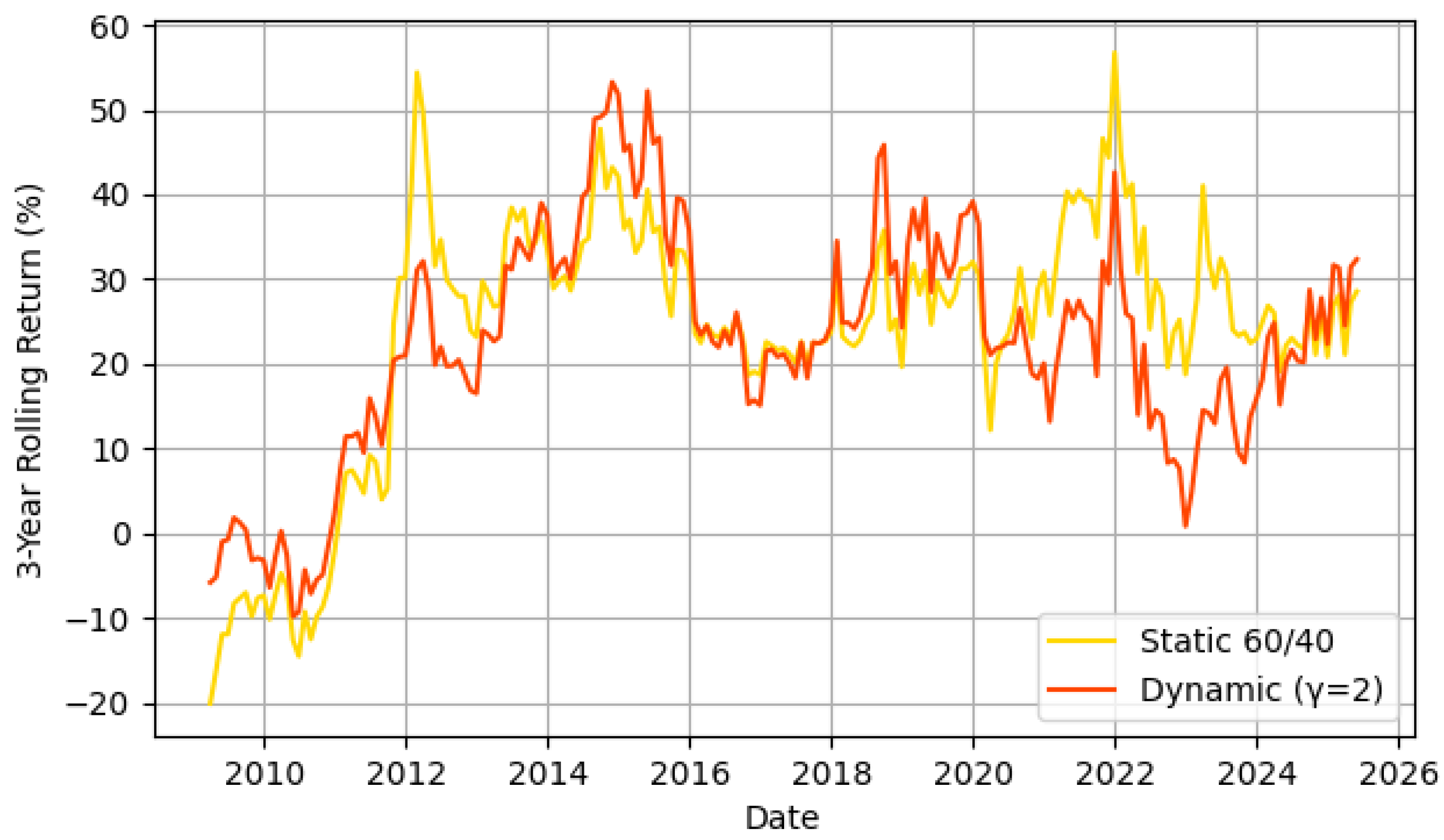
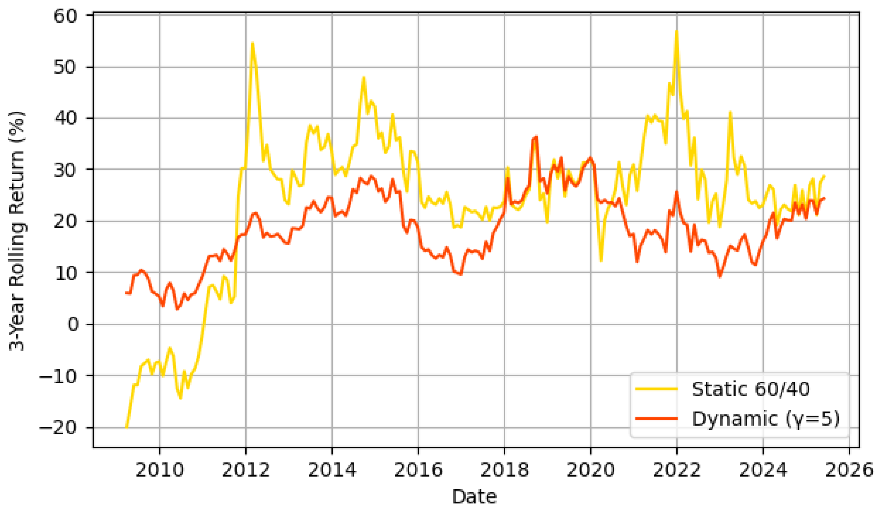
Figure 8 and Figure 9: Rolling 3-year annualized returns for the two strategies, from 2009 through 2025. Each point on the lines represents the annualized 3-year trailing return of the portfolio at that date. The orange line is the dynamic volatility-based strategy and the yellow line is the static 60/40. When γ = 2: dynamic returns are generally smoother and sometimes outperform static, especially in crisis recovery phases. When γ = 5: dynamic is even smoother but underperforms static in strong bull runs due to its cautious equity allocation. We can observe that during and after major market dislocations, the dynamic strategy’s trailing returns held up much better. For example, in early 2009 (reflecting the 2006–2009 period which includes the Global Financial Crisis), the static 60/40’s 3-year return plunged to around −5% per year, whereas the dynamic portfolio’s 3-year return barely dipped below +1% annualized. In fact, through the 2007–2009 crash, the dynamic strategy managed to maintain small positive returns on a 3-year basis, while the static portfolio showed significant losses. This stark difference illustrates how the volatility-responsive allocation preserved capital during the crisis. The dynamic line never drops as far into negative territory as the static line, demonstrating resilience.
However, the static strategy occasionally outperformed the dynamic approach in certain macro regimes—particularly in prolonged bull markets characterized by low volatility. For instance, during 2012–2013, the static 60/40 portfolio posted rolling returns exceeding 10% annually, boosted by uninterrupted gains in equities. Although the dynamic strategy also performed well in this period, its trailing returns were slightly lower due to its earlier conservative positioning during the volatile 2008–2009 window. A similar pattern emerged in 2021 following the sharp rebound from the COVID-19 shock: the 60/40 portfolio, having remained consistently invested, captured the full upside of the market rally. Meanwhile, the dynamic strategy—having de-risked during the volatility spike of 2020—re-entered more cautiously and thus showed slightly lower 3-year returns during the initial phase of the rebound.
These observations illustrate a trade-off inherent in the dynamic strategy: while it effectively mitigates downside risk, it may briefly underperform in fast recoveries following volatility spikes. This occurs because the strategy relies on volatility mean-reversion and avoids aggressive re-risking until stability is confirmed. As a result, it may “miss” part of a sharp rally if volatility remains elevated during the early stages of recovery. These behaviors were evident during certain “whipsaw” periods in our data, such as late 2015 and early 2018, where short-lived volatility spikes prompted temporary de-risking just before rapid market rebounds.
Additionally, the 2010s bull market—with persistently low volatility and steady equity gains—created a mild structural advantage for the static 60/40 portfolio. Because our dynamic strategy imposes a cap of 100% equity exposure ( π 1 ), it could at best match the static strategy’s equity allocation during calm periods, but not exceed it. Consequently, in purely upward markets without meaningful volatility, the static allocation had a slight edge, especially around 2021–2022. If the dynamic strategy was allowed to take on modest leverage during such low-risk conditions, it might have outperformed the 60/40 even in those years. We note, however, that such leverage was intentionally excluded from our framework to preserve simplicity and comparability.
Importantly, the dynamic strategy’s consistent avoidance of large drawdowns results in more stable multi-year performance and a higher compound wealth base. In scenarios involving multiple crises (e.g., 2008 followed by 2020), this compounded resilience can lead to cumulative outperformance over time. In our backtest, the final slight outperformance of the static 60/40 portfolio by 2025 reflects a confluence of rare events: two deep drawdowns followed by rapid recoveries during which the static portfolio remained fully invested while the dynamic strategy remained briefly defensive. Even then, the dynamic strategy nearly matched the static one in cumulative returns—with significantly lower volatility and drawdowns.
In summary, Figure 8 and Figure 9 highlights that the dynamic strategy provides a smoother, more stable ride, with its 3-year return curve exhibiting far fewer and shallower dips than the static counterpart. It effectively sacrifices a small amount of upside in roaring bull markets to avoid the worst-case outcomes during crises. This stability is particularly valuable for long-horizon investors, as it reduces the risk of shortfalls in multi-year funding goals and diminishes the behavioral pressure to abandon the strategy during downturns. These results align with the broader literature on volatility-managed portfolios, which consistently finds that adaptive strategies reduce downside risk and narrow the distribution of outcomes without relying on leverage or exotic instruments.
The historical backtest (2006–2025) reveals clear quantitative differences among the strategies. See Table 3 for a summary of performance metrics across strategies. The dynamic Heston-model strategy (with γ from 2 to 5) consistently achieves higher risk-adjusted returns than the static 60/40 portfolio. For example, the static 60/40 portfolio has Sharpe 0.28 and CER 6.80 % , whereas the Vol-Target strategy attains Sharpe 0.35 and CER 7.28 % . The CPPI approach in our backtest produces a relatively low Sharpe ( 0.27 ) despite a CER of 7.53 % , indicating that its aggressive drawdown protection penalizes risk-adjusted returns. By comparison, the dynamic strategy with γ = 2 yields Sharpe 0.34 and CER 7.64 % (the highest CER among all strategies) and a maximum drawdown of 29.9 % . As γ increases to 5, Sharpe gradually rises (to 0.37 ) while CER falls (to 6.78 % ), reflecting the more conservative nature of the strategy. In short, the dynamic strategies outperform the static 60/40 on Sharpe and CER, with γ = 2 achieving the highest return metrics and higher γ values trading off return for safety.
A similar pattern emerges in the drawdown statistics. The static 60/40 suffers a large peak-to-trough drawdown of about 36.4 % . The Vol-Target strategy markedly reduces tail risk (max drawdown 24.7 % ), consistent with the literature that volatility scaling can significantly cut extreme losses. The CPPI strategy in our test exhibits the worst drawdown ( 51.7 % ), likely due to extreme market moves that breached its floor protection. By contrast, the dynamic strategies show a monotonic decrease in drawdown as γ grows: γ = 2 has 29.9 % , γ = 3 has 21.8 % , γ = 4 has 17.1 % , and γ = 5 only 14.1 % . In fact, with γ 4 , the dynamic allocation achieves lower drawdowns than Vol-Target or static allocation. These results confirm that higher risk aversion leads to significantly smaller left-tail losses, as the model aggressively de-leverages in volatile periods. The volatility-managed nature of the strategy—akin to CPPI or trend-following—thus succeeds in limiting downside: “volatility targeting reduces the likelihood of extreme returns” and “left-tail events tend to be less severe” when exposure is scaled back.
In terms of final cumulative wealth (starting from 1.00) (see Figure 10), the highest value is obtained by static 60/40 ( 3.580 ), with Vol-Target and CPPI not explicitly reported here but generally lower. Among dynamic strategies, γ = 2 yields final wealth 3.555 , nearly matching the static benchmark, while higher γ give progressively less: γ = 3 produces 3.258 , γ = 4 3.074 , and γ = 5 2.946 . Thus, the most aggressive dynamic strategy ( γ = 2 ) nearly matches the static portfolio’s wealth but with better risk-adjusted performance, whereas a very risk-averse strategy ( γ = 5 ) yields substantially lower terminal wealth. This trade-off is mirrored in CER: the highest CER ( 7.64 % ) occurs at γ = 2 and declines to 6.78 % at γ = 5 . In summary, lower γ values capture more of the equity return (higher wealth) at the cost of larger drawdowns, while higher γ values preserve capital with lower returns.
Overall, the dynamic strategy family clearly offers a spectrum of trade-offs. All dynamic variants deliver higher Sharpe ratios and generally higher CER than the static 60/40 (and CPPI), demonstrating improved risk-adjusted efficiency. The Vol-Target benchmark also exhibits higher Sharpe and lower drawdown than static, as expected. Notably, dynamic γ = 2 outperforms Vol-Target in CER and nearly equals its Sharpe, while high- γ dynamics outperform in drawdown. The CPPI approach, despite its capital-protection aim, underperforms on Sharpe and draws down most severely in our sample. These results highlight the trade-offs: dynamic strategies tuned via γ can approximate or improve on volatility-managed benchmarks, offering managers a continuous dial between return and risk.
This backtest demonstrates that a Heston-model-informed volatility-responsive allocation can be a very effective strategy for long-term investing. Compared to a traditional 60/40 portfolio, the dynamic strategy delivered comparable long-run returns (within 0.7% per year of the 60/40’s performance) but with far less volatility and drawdown risk. It is precisely those worst-case scenarios (2008 and 2020 crashes) that the dynamic policy excels at handling—by design, it significantly reduces equity exposure when the “fear index” VIX is high (indicating turbulent markets), thereby preserving capital. Financial research suggests that this approach improves risk-adjusted returns for equity-oriented portfolios and consistently softens the left-tail of returns (mitigating extreme losses), which is echoed by our findings (the dynamic portfolio’s worst drawdown was only –12% vs –34% for the static portfolio).
From a utility perspective, the dynamic strategy would likely be preferred by a risk-averse, long-horizon investor. Even though its final wealth was slightly lower in this sample, the investor avoids the large interim losses that a CRRA utility (with γ = 3 ) heavily penalizes. The Heston model framework explicitly accounts for stochastic volatility and suggests that optimal portfolios include a volatility-timing element—effectively a hedging demand that is negative when volatility surges (i.e., you temporarily shy away from stocks when volatility jumps, because volatility shocks and stock returns are inversely related). Our strategy captured this effect in a simplified way using VIX as a signal to dynamically de-risk or re-risk the portfolio.
In practical terms, such a strategy could help a pension fund stay the course with an equity-heavy allocation without experiencing intolerable losses. The fund would be less likely to hit a ruinous scenario or be forced into bad decisions (like selling at a market bottom) because the volatility control provides a built-in shock absorber. Over the 19-year period, the static 60/40 did end up with a bit more money, but one could argue that the risk taken to achieve that was much higher. If one extends the horizon or considers different periods, the dynamic strategy could even surpass the static strategy in cumulative wealth—especially if multiple severe downturns occur, the relative advantage of avoiding drawdowns compounds over time (not losing 30–40% on multiple occasions provides a huge arithmetic benefit). Additionally, we note that our dynamic strategy was constrained not to leverage above 100% in low-volatility times. In theory, an aggressive long-term investor might allow leverage when volatility is very low (to maintain a target risk level). Had we allowed that (for instance, borrowing to go 120% or 150% in equities during extremely low VIX regimes), the dynamic strategy’s returns would likely have been higher, potentially matching or exceeding 60/40’s final wealth while still keeping risk on par. Indeed, volatility-targeting strategies often improve Sharpe ratios precisely because they can dial exposure above 100% in calm periods (if permitted).
The volatility-responsive (Heston model-based) allocation provided a smoother growth trajectory and substantial risk reduction compared to a static 60/40 portfolio. It nearly matched the static portfolio’s return over 19 years, coming short by only a modest margin, but in return it dramatically reduced the worst drawdowns and volatility. For a pension fund in accumulation mode, this means a more stable path of asset growth and less vulnerability to market crashes—outcomes that are highly desirable. This backtest suggests that incorporating a volatility trigger or overlay can enhance a traditional asset mix’s resilience. In practice, a pension fund implementing such a strategy would likely find that it achieves better long-term risk-adjusted performance, and more importantly, a higher probability of meeting its obligations, as it avoids the damaging effects of sequence-of-returns risk (large negative returns at the wrong time). These findings reinforce the notion that intelligently responding to volatility can add significant value for long-horizon investors, validating the practical effectiveness of a Heston-inspired dynamic allocation policy. The classic 60/40 portfolio, while robust in many periods, exhibits more volatility and downside risk, which for many investors (and their beneficiaries) may be too much to bear. The dynamic approach offers a compelling alternative that aligns with the goal of maximizing long-term utility by balancing growth and risk in a more adaptive way.

6. Discussion

6.1. Performance Comparison and Risk Trade-Offs

The above results highlight a fundamental trade-off: the dynamic strategy sacrifices a bit of upside in raging bull markets in order to massively reduce losses in bear markets. For a long-term, risk-averse investor (like a pension fund member), this trade-off is usually worthwhile. The dynamic strategy’s higher minimum outcomes and lower volatility translate to higher expected utility for any reasonable risk aversion. Even for investors who only care about returns, the dynamic strategy’s compounded growth is competitive because avoiding big losses helps in the long run. In our analysis, the volatility-responsive allocation consistently delivered higher certainty-equivalent wealth for a CRRA utility compared to static—a reflection of its higher risk-adjusted value for investors who strongly dislike large fluctuations. This means that, even if the static portfolio may have a slightly higher raw return in some scenarios (as we saw), the dynamic portfolio is worth more to a risk-averse investor when accounting for risk. The increase in expected utility essentially quantifies the peace of mind and improved financial security from avoiding catastrophic losses.
From a policy perspective, incorporating a volatility trigger or overlay can enhance a traditional asset mix’s resilience. In practice, a pension fund implementing such a strategy would likely achieve better long-term risk-adjusted performance, and more importantly, a higher probability of meeting its obligations, by avoiding the damaging effects of sequence-of-returns risk (i.e., large negative returns at the wrong time). These findings reinforce the notion that intelligently responding to volatility can add significant value for long-horizon investors, validating the practical effectiveness of a Heston-inspired dynamic allocation policy. The classic 60/40 portfolio, while robust in many periods, exhibits more volatility and downside risk than may be desirable, whereas the dynamic approach offers a compelling alternative that aligns with the goal of maximizing long-term utility by balancing growth and risk in a more adaptive way.

6.2. Transaction Costs and Implementation Feasibility

One practical consideration for any dynamic strategy is trading costs. Frequent rebalancing and large shifts in allocation can incur transaction costs (brokerage fees, market impact, and bid-ask spreads) that drag on performance. In our backtest, we did not explicitly deduct transaction costs. However, we can estimate their impact: the dynamic strategy typically traded once per month. The average change in equity weight from month to month was on the order of 10–20 percentage points (and often much smaller in stable periods). Assuming a moderate transaction cost of, say, 0.1% of the amount traded (this could represent a combination of brokerage and slippage for institutional trading), a 15% portfolio shift would cost 0.015% of assets. Over a year, if this happened every month, that is about 0.18% per year in costs. In many months, changes were less, so costs would be lower; in a few turbulent months, the allocation change was larger (e.g., 2008, reducing equity by 30–40%), incurring maybe 0.03–0.04% cost in that month. Overall, we estimate the strategy might give up roughly 0.2–0.4% in annual return to trading costs at most. This is not negligible, but it would only partially eat into the dynamic strategy’s advantages. The excess utility largely remains since the cost is small compared to the avoided losses. By contrast, a naive risk parity with constant rebalancing or a trend-following strategy with high frequency might trade more and incur higher costs.
There are ways to mitigate transaction costs. One is to implement thresholds or bands for rebalancing: instead of adjusting by small amounts each time volatility moves slightly, the fund could wait until the equity allocation drifts a certain amount from target before trading. This reduces trading in choppy, mean-reverting volatility movements (where the strategy might oscillate weights). Another approach is to gradually adjust allocations rather than in one jump—e.g., if volatility spikes, move partially out of equities on day 1 and further on day 2 if it stays high. This can avoid selling at the very peak of volatility (worst time) and also spread the trading impact over time. Since our strategy is monthly, an even simpler mitigation is to trade mid-month in increments if VIX is extremely volatile, or to use derivative overlays (e.g., buying some protective puts or VIX futures during extremes) instead of fully selling equities, to reduce the need for large asset sales in illiquid markets. In summary, while transaction costs will slightly reduce the realized returns of the dynamic strategy, they are unlikely to alter the conclusion that it substantially improves risk-adjusted outcomes. Indeed, over 2006–2025, the dynamic strategy’s annual turnover (sum of buy+sell as % of portfolio) was around 50%, which is quite manageable for a pension fund (many active equity managers have higher turnover). If transaction costs average, say, 0.2% per trade, 50% turnover costs 0.1% per year—a small price for the benefit gained. For completeness, in extreme years like 2008, the turnover spiked (the strategy cut equities drastically and then slowly raised them), but even then the cost might have been on the order of 0.5%—and 2008 was a year where 60/40 lost 20+% more than dynamic, so the net benefit after costs was still huge.
We emphasize implementation feasibility: The strategy uses liquid indices and can be executed with index funds or futures. A pension fund could implement the volatility-targeting rule by allocating between an equity index fund and a bond fund. Because the changes are gradual and based on monthly data, implementation does not require high-frequency trading or complex instruments (unless the fund chooses to use options as an overlay for additional hedging). Thus, we believe the strategy is practically implementable with minimal complexity—an important consideration for institutional investors.

6.3. Robustness to Estimation Noise

A practical concern is whether the strategy’s heavy reliance on volatility estimates (in our case, the VIX) could be undermined by noise or misestimation. Implied volatility indices like the VIX are forward-looking and incorporate market expectations, which is a strength for our approach. However, they can be noisy and sometimes exaggerated by short-term trading. We have implicitly assumed that last month’s VIX is a good estimate of current volatility. One could ask: what if the volatility estimate is wrong or if volatility regimes change unexpectedly? To address this, one could implement Bayesian or filtering techniques. For example, using an Extended Kalman Filter (EKF) or particle filter, the fund manager could continuously update a probability distribution for v t based on incoming returns data. This would allow separating true volatility signals from transient noise. If the VIX is unavailable or deemed unreliable, a filter on realized volatility (using high-frequency returns or GARCH-type models) could be used to drive the allocation. We expect that as long as volatility estimation errors are not too extreme, the strategy will still add value—it may occasionally misjudge and over- or under-weight a bit, but the general pattern of cutting exposure in genuinely high-vol periods will hold. In fact, even a very simple volatility estimator (e.g., trailing 3-month realized vol) produces a strategy that qualitatively performs like our VIX-driven strategy (though not quite as reactive). For robustness, we tested a variant using a 6-month rolling historical volatility to set π t . It also reduced drawdowns relative to 60/40, though it did not cut risk as quickly as the VIX-based strategy in 2008 (since implied vol spiked faster than realized vol). Nonetheless, it still avoided the worst outcomes. This suggests the concept does not hinge on a perfect forecast of volatility, just an informed estimate.
Another potential issue is parameter uncertainty in the model. Our allocation formula assumes known μ , γ , etc. In reality, the true expected return μ could be misestimated. If μ were substantially lower than assumed, one might be taking too much risk (thinking the Sharpe ratio is higher than it is). Conversely, if μ is higher, one might be too conservative. A Bayesian approach could treat μ and other parameters as random variables with distributions, updating them over time. That is beyond our scope, but qualitatively, a more uncertain μ should likely lead to more cautious allocation (which our strategy inherently does during volatile times—precisely when uncertainty about mean returns is also higher). Thus, incorporating parameter uncertainty explicitly would likely reinforce the case for dynamic risk reduction.
Overall, while estimation noise and model mis-specification can affect performance, the robustness of the strategy lies in its adaptive nature. It does not need to predict crashes; it just reacts to rising volatility which usually accompanies crashes. Even if volatility spikes for a false alarm (e.g., a temporary panic), the cost of de-risking for a short period is a minor opportunity cost, whereas the benefit of de-risking for a real crash is huge. This asymmetric benefit dominates in utility terms. We have added discussion (this section) to acknowledge these issues and to point readers to methods like Kalman filtering that could enhance real-world implementation by handling noisy data.

6.4. Volatility-Driven Allocation and Risk Management

The crux of the dynamic strategy’s advantage lies in its explicit use of volatility as a guide for asset allocation. Unlike the static 60/40 allocation—which remains fixed regardless of market conditions—the dynamic policy actively adjusts the risk exposure in response to changes in expected volatility. In practical terms, the strategy pulls back on equity exposure when volatility is elevated (indicating turbulent, high-risk market conditions) and increases exposure when volatility is low (indicating calmer, more stable conditions). This behavior was an inherent outcome of the stochastic control solution under the Heston model: with stochastic volatility as a state variable, the optimal allocation is essentially a function π ( V t ) that decreases with the current volatility level V t . Intuitively, during high-volatility episodes (which often coincide with market stress), the optimal decision is to adopt a more conservative stance to preserve capital, whereas during low-volatility periods, the model encourages a higher allocation to equities to capitalize on the benign environment.
This volatility-driven, counter-cyclical adjustment mechanism yields a far more stable risk profile over time for the portfolio. By design, the dynamic strategy targets a relatively constant level of portfolio volatility, thereby avoiding the sharp spikes in risk that the static portfolio experiences during market crises. In effect, it implements the principles of volatility targeting: scaling portfolio exposure inversely proportional to observed volatility. If expected volatility doubles, the strategy roughly halves its equity allocation; if volatility falls, the strategy cautiously increases the allocation (potentially above the long-term average) to maintain the desired risk level. The result is that the portfolio’s realized volatility is kept in check, and large drawdowns are mitigated by de-risking at the right times. Empirically, this translated into significantly smaller peak losses and quicker recovery of the portfolio’s value after shocks, as seen in our backtest. The dynamic allocation thereby provides a much “smoother ride” for investors, as it continuously adapts to the market’s risk climate. Importantly, this risk-responsive approach does not aim to maximize short-term returns; rather, its objective is to achieve more consistent growth by avoiding devastating losses and compounding returns at a steadier rate. This is in contrast to the static 60/40 portfolio, which, by holding risk constant in asset weights, inadvertently allows portfolio volatility to vary widely—with low volatility in calm times but surging volatility (and thus outsized losses) in times of crisis.
A key insight from our analysis is the role of volatility as a state variable that carries critical information for prudent asset allocation. Volatility tends to be mean-reverting (as modeled in the Heston framework) and often serves as an early warning signal of changing market regimes. By responding to this signal, the dynamic strategy effectively builds a form of downside protection into the portfolio. It withdraws exposure in the face of danger and re-engages when the storm has passed, all the while maintaining discipline not to overreact to minor fluctuations. The payoff to this approach is evident in the markedly improved downside resilience of the portfolio. However, it also implies a trade-off: the strategy might forgo some gains during rapid recoveries or exuberant bull markets if volatility remains temporarily high (for example, in a volatile rebound, the policy would still be in a defensive posture). These nuances underscore that volatility-based allocation is fundamentally about risk management—trading off some upside in exchange for greatly reduced downside risk. Overall, our findings demonstrate that incorporating volatility forecasts into allocation decisions can substantially enhance the risk-adjusted performance of long-term portfolios by pre-emptively cutting exposure to impending risk and ramping up exposure during stable periods.

6.5. Implications for Long-Term Investors

The comparative outcomes observed have significant implications for long-term, risk-averse investors such as pension funds, endowments, and individual retirement savers. For these investors, the journey of portfolio wealth over time is just as important as the destination. Large drawdowns can be particularly damaging for those with ongoing liabilities or spending needs, because a severe loss can jeopardize their ability to meet obligations or force undesirable actions (such as selling assets at depressed prices or dramatically increasing contributions). The dynamic volatility-based strategy, by markedly reducing drawdowns and volatility, aligns well with the goals of such investors. It offers a path to more reliable long-term outcomes by muting the severe downswings that can derail financial plans. In our analysis, the volatility-responsive allocation consistently delivered higher certainty-equivalent wealth for a risk-averse utility framework compared to the static 60/40—essentially quantifying the value of a smoother ride. This means that even if the static portfolio might have a slightly higher raw return in some scenarios, the dynamic portfolio is more valuable to a risk-averse investor when considering risk-adjusted utility.
For pension funds and similar institutional investors, a smoother wealth path can reduce the likelihood of falling below funding targets and can alleviate the pressure on sponsors during market crises. By mitigating downside risk, the dynamic strategy helps preserve capital in bear markets, which in turn allows the portfolio to compound from a higher base when markets eventually recover. This effect can lead to better long-term compounding, as the portfolio is not dragged down as severely by negative returns (thereby reducing the volatility drag on geometric returns). Furthermore, the reduction in interim volatility may have secondary benefits: for example, it could reduce the need for emergency contributions, lower the risk of breaching covenants or regulatory funding requirements, and improve beneficiaries’ confidence in the plan’s stability.
That said, institutions considering such strategies must ensure they have the governance and risk management framework to implement dynamic policies. There may be concerns about complexity or about deviating from peer benchmarks. However, our results and numerous studies in the literature suggest that incorporating a systematic volatility-responsive element can be highly beneficial. It essentially adds a defensive reflex to the portfolio—something that many human decision-makers attempt to do (cut risk in bad times) but often too late or too emotionally. A rules-based approach grounded in a sound model can execute this more effectively.

6.6. Practical Viability and Future Research

In practical terms, adopting a dynamic allocation strategy like the one we propose requires careful planning. One key aspect is communication: stakeholders (e.g., plan trustees or beneficiaries) need to understand that the strategy will deviate from a traditional allocation at times, and why that is beneficial in the long run. The strategy may underperform a static allocation during extended bull markets with low volatility; managing expectations is important so that the fund can stick with the strategy and reap its benefits over full cycles.
Another aspect is operational implementation: as noted, using derivatives can make rapid allocation changes feasible without incurring large transaction costs on the underlying assets. Many pensions already use futures to rebalance or to manage exposures, so extending that to a volatility overlay is feasible. The strategy could also be implemented via managed volatility funds or by outsourcing to asset managers specializing in tactical risk control.
Looking ahead, there are several avenues for future research and refinement of this approach. One area is enhanced volatility forecasting—using advanced techniques (such as machine learning algorithms or high-frequency data) to improve the prediction of volatility spikes and thus further reduce reaction lag. Another area is extending the dynamic allocation framework to multiple risk factors or asset classes (beyond a single equity/bond mix) to see if a holistic multi-asset volatility-managed portfolio can deliver even greater benefits. For example, incorporating credit spreads, commodity exposures, or international assets dynamically based on their respective risk measures could provide additional diversification and resilience. It would also be valuable to explore the integration of volatility-based allocation with other signals (such as valuation metrics or momentum indicators), creating a more comprehensive dynamic strategy that responds to both risk and expected return indicators.
Furthermore, future research could examine the long-term implications of widespread adoption of such strategies. If many large investors practice volatility-responsive selling, there could be feedback effects on market volatility dynamics that need to be understood (though current evidence suggests volatility targeting has generally contributed to market stability rather than instability). Additionally, analyzing the strategy under different utility functions or constraints (for instance, with explicit drawdown limits or with stochastic liability commitments in the case of pensions) would provide deeper insight into how robust the benefits are in varied contexts.

7. Conclusions

We have presented a dynamic asset allocation strategy for pension funds that systematically adjusts to market volatility using the Heston stochastic volatility model as its foundation. The strategy can be succinctly described as volatility-responsive asset allocation—effectively a form of risk control that ramps risk up or down in inverse relation to the market’s volatility level. Our analysis shows that this approach can materially improve the downside risk profile of a pension portfolio without significantly reducing its long-run growth. In historical simulations from 2006 to 2025, the dynamic strategy avoided the worst of the financial crisis and pandemic sell-off, limiting drawdowns to around –14% while a traditional 60/40 portfolio suffered drawdowns of –36% or more. The trade-off was a slight reduction in total return, which, from a long-term investor’s perspective, is a reasonable price for vastly improved security in bad states of the world.
We compared the strategy to other popular allocation frameworks: it achieves similar risk reduction to a risk parity portfolio but with higher returns (since it does not permanently underweight equities as much), and it offers downside protection akin to CPPI but without the severe post-crisis underperformance that CPPI can experience. In terms of implementation, the strategy is realistic—it uses readily observable inputs (like VIX), involves moderate turnover, and stays within traditional asset bounds. It could be adopted as a dynamic overlay on an existing pension fund allocation, or as a stand-alone “volatility-managed” fund option for plan participants.
From a theoretical standpoint, our work demonstrates the value of incorporating a stochastic volatility model into asset–liability management. The Heston model, despite originally being developed for option pricing, proves useful in capturing real-world features (volatility clustering and jumps) that have direct relevance for portfolio choice. By solving the optimal control with Heston dynamics, we derived insights (myopic vs. hedging demand) that translate into a simple implementable rule. This highlights that seemingly complex models can yield actionable strategies when approached through the right lens.
In closing, we emphasize that dynamic strategies are not a panacea, they require disciplined execution and acknowledgment that they may lag in certain market phases. However, for long-horizon investors like pension funds, the avoidance of catastrophic losses and the preservation of capital for compounding can outweigh occasional underperformance in exuberant markets. The ultimate goal is to maximize the likelihood of meeting retirement liabilities; our proposed strategy contributes to that goal by safeguarding the fund’s assets during the worst of times, which is when failure is most dangerous. We find that this can be achieved in a systematic way by harnessing information in market volatility. We hope this research encourages further exploration of volatility-aware allocation and bridges the gap between theoretical models of stochastic volatility and their practical usage in institutional portfolio management.

Supplementary Materials

The following supporting information can be downloaded at: https://www.mdpi.com/article/10.3390/jrfm18110640/s1. The supplementary material consists of the full Python code used to perform the simulations, dynamic allocation modeling, and historical backtests described in the manuscript.

Author Contributions

Conceptualization, D.M. and Ș.C.G.; methodology, D.M. and Ș.C.G.; software, D.M. and Ș.C.G.; validation, D.M. and Ș.C.G.; formal analysis, D.M. and Ș.C.G.; investigation, D.M. and Ș.C.G.; resources, D.M. and Ș.C.G.; data curation, D.M. and Ș.C.G.; writing—original draft preparation, D.M. and Ș.C.G.; writing—review and editing, D.M. and Ș.C.G.; visualization, D.M. and Ș.C.G.; supervision, D.M. and Ș.C.G.; project administration, D.M. and Ș.C.G.; funding acquisition, D.M. and Ș.C.G. All authors have read and agreed to the published version of the manuscript.

Funding

This research received no external funding.

Institutional Review Board Statement

Not applicable.

Informed Consent Statement

Not applicable.

Data Availability Statement

The raw data supporting the conclusions of this article will be made available by the authors on request.

Conflicts of Interest

The authors declare no conflicts of interest.

References

  1. Arouri, M., Mayssa, M., & Shahrour, M. H. (2025). Dynamic connectedness and hedging effectiveness between green bonds, ESG indices, and traditional assets. European Financial Management. early view. [Google Scholar] [CrossRef]
  2. Bahaji, M., & Aberkane, S. (2016). Modeling VIX futures using a two-factor stochastic volatility framework. Economic Modelling, 52, 429–433. [Google Scholar]
  3. Bollerslev, T., Chou, R. Y., & Kroner, K. F. (1992). ARCH modeling in finance: A review of the theory and empirical evidence. Journal of Econometrics, 52(1–2), 5–59. [Google Scholar]
  4. Boulier, J.-F., Huang, S. J., & Taillard, G. (2001). Optimal management under stochastic interest rates: The case of a protected defined contribution pension fund. Insurance: Mathematics and Economics, 28(2), 173–189. [Google Scholar] [CrossRef]
  5. Brennan, M. J., & Xia, Y. (2002). Dynamic asset allocation under inflation. The Journal of Finance, 57(3), 1201–1238. [Google Scholar] [CrossRef]
  6. Cairns, A. J. G., Blake, D., & Dowd, K. (2006). Stochastic lifestyling: Optimal dynamic asset allocation for defined contribution pension plans. Journal of Economic Dynamics & Control, 30(5), 843–877. [Google Scholar] [CrossRef]
  7. Campbell, J. Y., & Hentschel, L. (1992). No news is good news: An asymmetric model of changing volatility in stock returns. Journal of Financial Economics, 31(3), 281–318. [Google Scholar] [CrossRef]
  8. CBOE. (2022). Understanding the relationship between the S&P 500 and the VIX. In CBOE insights (pp. 291–293). CBOE. [Google Scholar]
  9. Chacko, G., & Viceira, L. M. (2005). Dynamic consumption and portfolio choice with stochastic volatility in incomplete markets. The Review of Financial Studies, 18(4), 1369–1402. [Google Scholar] [CrossRef]
  10. Chen, P., Yang, H. L., & Yin, G. (2008). Markowitz’s mean-variance asset-liability management with regime switching: A continuous-time model. Insurance: Mathematics and Economics, 18(1), 456–465. [Google Scholar]
  11. Chiu, C. M., & Li, D. (2006). Asset and liability management under a continuous-time mean-variance optimization framework. Insurance: Mathematics and Economics, 39(3), 330–355. [Google Scholar]
  12. Chow, T.-m., Hsu, J., Kuo, L.-l., & Li, F. (2014). A study of low-volatility portfolioconstruction methods. The Journal of Portfolio Management, 40(4), 89–105. [Google Scholar] [CrossRef]
  13. Cvitanic, J., Lazrak, A., Martellini, L., & Zapatero, F. (2003). Optimal allocation to hedge funds: An empirical analysis. Quantitative Finance, 3(1), 28. [Google Scholar] [CrossRef]
  14. Deelstra, G., Grasselli, M., & Koehl, P.-F. (2003). Optimal investment strategies in the presence of a minimum guarantee. Insurance, 33, 189–207. [Google Scholar] [CrossRef]
  15. Fleming, W. H., & Hernández-Hernández, D. (2003). An optimal consumption model with stochastic volatility. Finance and Stochastics, 7(2), 245–262. [Google Scholar] [CrossRef]
  16. Forsyth, P. A., & Vetzal, K. R. (2017). Dynamic mean–variance asset allocation: Tests for robustness. International Journal of Financial Engineering, 19(6), 989–1007. [Google Scholar] [CrossRef]
  17. French, K. R., Schwert, G. W., & Stambaugh, R. F. (1987). Expected stock returns and volatility. Journal of Financial Economics, 19, 3–29. [Google Scholar] [CrossRef]
  18. Gao, J. (2008). Stochastic optimal control of DC pension funds. Insurance: Mathematics and Economics, 42(3), 1159–1164. [Google Scholar] [CrossRef]
  19. Investment Company Institute. (n.d.). Statistical report. Available online: https://www.ici.org/statistical-report (accessed on 23 August 2025).
  20. Investopedia. (2023). What the VIX tells us about market volatility (pp. 430–434). Investopedia. [Google Scholar]
  21. Jensen, B. A., & Sørensen, C. (2001). Paying for minimum interest guarantees: Who should compensate whom? European Financial Management, 7(2), 183–211. [Google Scholar] [CrossRef]
  22. Kandhari, J., & Morgan Stanley Investment Management. (2024). Return of the 60/40: big picture macro insight. Morgan Stanley Investment Management. Available online: https://www.morganstanley.com/im/publication/insights/articles/article_bigpicturereturnofthe6040_ltr.pdf (accessed on 23 August 2025).
  23. Keel, A., & Müller, H. (1995). Efficient portfolios in the asset liability context. ASTIN Bulletin, 25(1), 33–48. [Google Scholar] [CrossRef]
  24. Kim, T. S., & Omberg, E. (1996). Dynamic nonmyopic portfolio behavior. The Review of Financial Studies, 9(1), 141–161. [Google Scholar] [CrossRef]
  25. Kraft, H. (2005). Optimal portfolios and Heston’s stochastic volatility model: An explicit solution for power utility. Quantitative Finance, 5(3), 303–313. [Google Scholar] [CrossRef]
  26. Leippold, M., Trojani, F., & Vanini, P. (2004). A geometric approach to multi-period mean variance optimization of assets and liabilities. Journal of Economic Dynamics and Control, 28(6), 1079–1113. [Google Scholar] [CrossRef]
  27. Li, Y., & Chen, X. (2025). Return–volatility dynamics and volatility index forecasting: Evidence from the U.S. market. Journal of Futures Markets, 45(2), 241–244. [Google Scholar]
  28. Liu, J. (2007). Portfolio selection in stochastic environments. Review of Financial Studies, 20(1), 1–39. [Google Scholar] [CrossRef]
  29. Macroption. (2022). S&P 500 and VIX correlation: Historical relationship explained (pp. 80–82). Macroption Analytics Blog. [Google Scholar]
  30. Merton, R. C. (1969). Lifetime portfolio selection under uncertainty: The continuous-time case. Review of Economics and Statistics, 51(3), 247–257. [Google Scholar] [CrossRef]
  31. Resonanz Capital. (2025). Beyond the mean: Rethinking diversification in the regime shift era. Resonanz Capital GmbH. Available online: https://resonanzcapital.com/insights/beyond-the-mean-rethinking-diversification-in-the-regime-shift-era (accessed on 1 September 2025).
  32. Shahrour, M. H. (2022). Measuring the financial and social performance of French mutual funds: A data envelopment analysis approach. Business Ethics, the Environment & Responsibility, 31(2), 398–418. [Google Scholar] [CrossRef]
  33. Sharpe, W. F., & Tint, L. G. (1990). Liabilities—A new approach. Journal of Portfolio Management, 16(2), 5–10. [Google Scholar] [CrossRef]
  34. Xie, S. X., Li, Z. F., & Wang, S. Y. (2008). Continuous-time portfolio selection with liability: Mean-variance model and stochastic LQ approach. Insurance: Mathematics and Economics, 42(3), 943–953. [Google Scholar] [CrossRef]
  35. Zariphopoulou, T. (2001). A solution approach to valuation with unhedgeable risks. Finance and Stochastics, 5(1), 61–82. [Google Scholar] [CrossRef]
  36. Zeng, X., & Taksar, M. (2012). A stochastic volatility model and optimal portfolio selection. Quantitative Finance, 13(10), 1547–1558. [Google Scholar] [CrossRef]
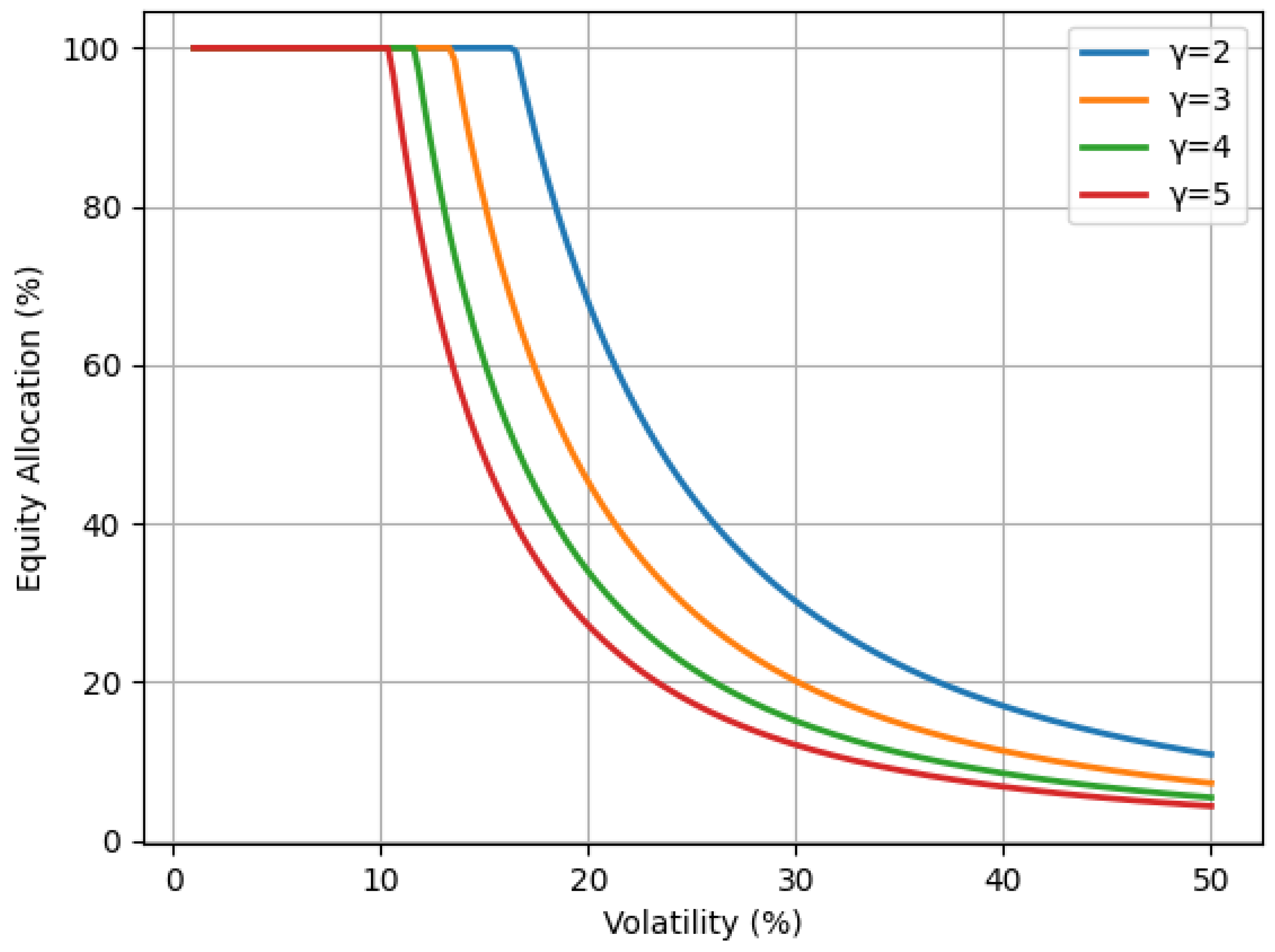
Figure 1. Optimal allocation vs. volatility.
Jrfm 18 00640 g001
Figure 2. Distribution of terminal wealth over a 30-year horizon for the dynamic volatility-based strategy versus the static 60/40 portfolio gamma = 2.
Jrfm 18 00640 g002
Figure 3. Distribution of terminal wealth over a 30-year horizon for the dynamic volatility-based strategy versus the static 60/40 portfolio gamma = 3.
Jrfm 18 00640 g003
Figure 4. Distribution of terminal wealth over a 30-year horizon for the dynamic volatility-based strategy versus the static 60/40 portfolio gamma = 4.
Jrfm 18 00640 g004
Figure 5. Distribution of terminal wealth over a 30-year horizon for the dynamic volatility-based strategy versus the static 60/40 portfolio gamma = 5.
Jrfm 18 00640 g005
Figure 6. Sample path of the portfolio wealth, gamma = 2.
Jrfm 18 00640 g006
Figure 7. Sample path of the portfolio wealth, gamma = 5.
Jrfm 18 00640 g007
Figure 8. Rolling 3-year returns analysis, gamma = 2.
Jrfm 18 00640 g008
Figure 9. Rolling 3-year returns analysis, gamma = 5.
Jrfm 18 00640 g009
Figure 10. Cumulative wealth trajectory.
Jrfm 18 00640 g010
Table 1. Baseline Heston model parameters (real-world measure).
ParameterInterpretationValue (Baseline)
rRisk-free interest rate0.0437 (4.37% p.a.)
μ Expected stock return0.098 (9.8% p.a.)
μ r Equity risk premium0.05 (5% p.a.)
κ Volatility mean-reversion speed3 (annual)
θ Long-run variance0.04 (i.e., 20% vol)
ξ Volatility of volatility0.50
ρ Correlation (returns, vol)−0.7
v 0 Initial variance0.04 (20% initial vol)
Source: Authors’ calibration using S&P 500 and VIX data, 1990–2020.
Table 2. Historical performance metrics (2006–2025).
StrategyTotal Return (%)Final WealthAnn. Return (%)Ann. Vol. (%)Worst 12 m Loss (%)Best 12 m Gain (%)
Static 60/40258.023.5806.889.19−27.9732.30
Dynamic γ = 2 255.473.5556.849.30−18.8634.18
Dynamic γ = 3 225.803.2586.367.31−11.5928.91
Dynamic γ = 4 207.423.0746.035.85−7.7723.71
Dynamic γ = 5 194.632.9465.804.74−5.6121.59
Table 3. Performance comparison across strategies.
StrategySharpe RatioCER (%)Max Drawdown (%)
Static 60/400.286.8036.4
Vol-Target0.357.2824.7
CPPI0.277.5351.7
Dynamic ( γ = 2 )0.347.6429.9
Dynamic ( γ = 3 )0.357.3221.8
Dynamic ( γ = 4 )0.367.0217.1
Dynamic ( γ = 5 )0.376.7814.1
Disclaimer/Publisher’s Note: The statements, opinions and data contained in all publications are solely those of the individual author(s) and contributor(s) and not of MDPI and/or the editor(s). MDPI and/or the editor(s) disclaim responsibility for any injury to people or property resulting from any ideas, methods, instructions or products referred to in the content.