Abstract
Modern credit scoring systems must operate under increasingly complex borrower data conditions, characterized by structural heterogeneity and regulatory demands for transparency. This study proposes a modular modeling framework that addresses both interpretability and data incompleteness in credit risk prediction. By leveraging Weight of Evidence (WoE) binning and logistic regression, we constructed domain-specific sub-models that correspond to different attribute sets and integrated them through ensemble, hierarchical, and stacking-based architectures. Using a real-world dataset from the American Express default prediction challenge, we demonstrate that these modular architectures maintain high predictive performance (test Gini > 0.90) while preserving model transparency. Comparative analysis across multiple architectural designs highlights trade-offs between generalization, computational complexity, and regulatory compliance. Our main contribution is a systematic comparison of logistic regression–based architectures that balances accuracy, robustness, and interpretability. These findings highlight the value of modular decomposition and stacking for building predictive yet interpretable credit risk models.
1. Introduction
Credit scoring models serve as the foundation of risk management in modern banking, enabling financial institutions to estimate the probability of default (PD) and optimize capital allocation under regulatory frameworks such as Basel III (Fidrmuc & Lind, 2020). However, real-world banking environments present a fundamental challenge: borrower data is inherently heterogeneous, with individuals providing diverse and often non-overlapping combinations of attributes. For instance, one applicant might supply comprehensive credit history and employment records, while another offers only transaction data and demographic information. This structural heterogeneity differs fundamentally from simple missing data problems as it reflects genuine variability in customer profiles rather than random omissions (Tarka, 2018; Scheres, 2010). Traditional credit scoring models (West, 2000), designed for fixed feature sets, struggle with this complexity. Common workarounds like imputation introduce bias, while excluding incomplete cases leads to information loss—particularly problematic as digital banking and alternative data sources expand the range of customer profiles (Van Ginkel et al., 2020).
The challenge extends beyond technical modeling to regulatory compliance. While machine learning advances have improved predictive accuracy, many state-of-the-art models operate as “black boxes,” conflicting with financial regulations that demand transparency (e.g., GDPR’s “right to explanation”) and fairness (e.g., the U.S. Fair Lending Act; U.S. Department of Housing and Urban Development, 2009). This tension between accuracy and interpretability has paralyzed practical adoption, leaving banks to choose between regulatory compliance and predictive performance.
This paper bridges this divide through a modular architecture that harmonizes three critical requirements: (1) handling heterogeneous attribute sets natively, (2) maintaining interpretability for regulatory compliance, and (3) achieving robust predictive performance. Our approach combines Weight of Evidence (WoE) optimal binning—which explicitly treats missing attributes as informative signals—with dynamically assembled logistic regression sub-models. The system trains specialized models for each observed attribute combination (e.g., A,B, B,D) and integrates them through stacking or hierarchical ensembles, preserving interpretability at each stage. Empirical validation on an American Express benchmark dataset demonstrates that this architecture achieves exceptional discrimination (Gini > 0.90) while providing the transparency needed for regulatory audits and customer explanations.
The main contributions of this study are threefold. First, we introduce a modular decomposition of customer financial behavior into delinquency, spending, payments, balances, and risk modules, which allows for both interpretability and targeted model evaluation. Second, we provide a systematic comparison of several logistic regression–based architectures, including single models, multi-model subsets, hierarchical combinations, and ensemble methods. Third, we demonstrate that stacking ensembles built on these modules substantially improve predictive power while maintaining interpretability, achieving state-of-the-art performance on the American Express dataset. Together, these contributions advance the design of credit risk models by balancing accuracy, robustness, and transparency.
Related Work
Traditional credit scoring models fall into two interpretable categories: parametric and rule-based. Logistic regression (Martens et al., 2007), the industry standard for decades, offers transparency through linear coefficients but fails to capture non-linear relationships without manual feature engineering. Decision trees (Appiahene et al., 2020) improve flexibility through recursive partitioning but tend to overfit with high-dimensional data. Rule-based systems (Lee, 2008), while intuitively interpretable, require constant updates to remain accurate and scale poorly to complex datasets.
Modern approaches attempt to balance flexibility and interpretability but face distinct limitations. Generalized Additive Models (GAMs; Hastie, 2017) relax linearity assumptions through smooth functions but become computationally prohibitive with many features. Bayesian Networks (Ben-Gal, 2008) explicitly model feature dependencies via directed graphs but require either expert-defined structures or expensive learning algorithms. Attention mechanisms in neural networks (Van Ginkel et al., 2020) provide post hoc explanations via feature importance weights but remain fundamentally opaque due to their deep learning foundation.
Hybrid and ensemble methods have emerged as compromise solutions. Random Forests (Cutler et al., 2012) aggregate multiple decision trees to reduce variance while offering feature importance scores, though these provide only global—not instance-level—interpretability. Recent hybrid architectures combine traditional models (e.g., logistic regression) with neural feature extractors (Olaniran et al., 2025), but their two-stage designs complicate regulatory validation. Crucially, none of these approaches address the core challenge of heterogeneous attribute sets natively. Most either impute missing values, introducing well-documented biases, or discard incomplete cases, wasting potentially predictive information.
Our work advances the field by unifying three typically disjoint strands of research: interpretable modeling, ensemble learning, and missing-data theory. Unlike imputation-based approaches, we treat attribute availability patterns as informative signals. In contrast to monolithic deep learning models, our modular design embeds interpretability at every level, from WoE-binned features to logistic regression coefficients. The architecture’s dynamic sub-model selection also addresses a practical industry pain point: banks can incorporate new data sources without retraining entire systems, significantly reducing maintenance costs compared to fixed-feature models (Mahadevan & Mathioudakis, 2023).
2. Methodology
This section outlines the systematic approach taken to develop interpretable classification models for predicting the probability of default (PD) in banking systems using a dataset from Kaggle. The dataset is divided into several modules, each representing a distinct set of attributes. The methodology is structured into several key steps: data preprocessing, single-factor analysis, multi-factor analysis, model candidate selection, architecture designs, evaluation, and comparison. The goal is to create modular architectures based on logistic regression and compare their performance using various metrics and statistical tests.
2.1. Data Preprocessing
2.1.1. Dataset Description
The dataset used in this study originates from the American Express Default Prediction competition hosted on Kaggle (2022). It contains anonymized, customer-level information aggregated at a monthly level over an 18-month observation window. The target variable is binary, where a value of 1 indicates that the customer defaulted on payment within 120 days of their latest statement date.
The dataset includes five major modules of features, each describing different aspects of customer financial behavior:
- Delinquency (D_*): Indicators of late or missed payments, e.g., number of overdue installments or historical delinquency counts.
- spending (S_*): Measures of transaction volume and frequency, capturing overall consumption behavior and trends.
- payments (P_*): Features related to payment amounts, payment-to-balance ratios, and payment regularity.
- balances (B_*): Measures of credit utilization, outstanding balances, and revolving amounts.
- risks (R_*): Aggregated risk-related indicators, e.g., derived scores or ratios reflecting risk exposure.
In addition, the dataset includes 11 categorical features that capture structural customer-level attributes not directly linked to monthly numeric flows. These features include identifiers and categorical risk flags such as B_30, D_63, and D_68. While anonymized, they typically correspond to customer profile categories such as product type, account status, or delinquency classification. For example, D_63 and D_68 are categorical delinquency flags, while B_30 represents a categorical balance-related status. The remaining categorical variables serve as segmentation markers (e.g., risk groups and account conditions) that are crucial for model interpretability since they allow the model to distinguish between different borrower profiles even when numerical behavior is similar.
In total, the dataset provides a rich and heterogeneous set of customer-level features, comprising both numeric and categorical information. This structure allows the proposed modular architectures to evaluate predictive power across different behavioral dimensions while preserving interpretability.
2.1.2. Handling Missing Values
In the preprocessing stage, categorical variables were grouped into bins according to the frequency of their occurrence. Categories with sufficient representation were retained as individual bins, while infrequent categories were aggregated into a common other bin. For missing values, a dedicated missing bin was introduced. In cases where more than one category is simultaneously missing for a given observation, the record is still assigned to the same missing bin. This ensures a consistent treatment of missingness across all variables and prevents unnecessary sparsity from creating separate bins for multi-category missing cases.
It should be noted that in this context, the term bin refers to the statistical grouping of categories or numerical ranges that share similar characteristics. It does not denote a computational module or software component but rather a data-driven grouping strategy used to reduce sparsity and improve model interpretability.
2.1.3. Data Splitting
The dataset is split into 2 (training (70% dev), test (30% dev)) sets to ensure robust evaluation of the models.
2.2. Optimal Binning Using Weight of Evidence (WoE)
The goal of best binning analysis is to categorize a set of variables and the values of each variable into a set of bins to achieve classification results maximization for each variable’s information and to satisfy interpretability and industry business logic using bins. By binning all the variables in the data, the relationship between the attribute and the target variable (default/non-default) is more clear and more tractable. The binned categories are optimal in capturing the maximum significance to the target through its use of Weight of Evidence (WoE) and eventually increasing the predictive power of the model.
Weight of Evidence (WoE) Definition and Formulas:
The Weight of Evidence (WoE) measures the strength of the relationship between a predictor variable and a binary target (e.g., default/non-default). It is calculated for each bin i as
where
- Proportion of Non-Defaults in Bin i
- Proportion of Defaults in Bin i
Interpretation: WoE Positive values indicate lower risk, and negative values indicate higher risk.
The Weight of Evidence (WoE) optimal binning technique is applied to variables within each module. This method groups values into discrete bins based on their WoE, which measures the strength of the relationship between the attribute and the target variable. The WoE for each bin is calculated as the natural logarithm of the ratio of the proportion of non-defaults to defaults within that bin. The binning process ensures a monotonic relationship between the binned variable and the target, which is critical for interpretability and model stability. In the end, missing values are assigned to a separate bin, ensuring that they are explicitly handled and contribute meaningfully to the analysis.
Each continuous attribute is transformed into a WoE variable with optimal bins, where each bin represents a range of values with a distinct WoE. These binned variables are now ready for single-factor analysis, providing a clear and interpretable representation of the relationship between the attribute and the target variable. The WoE values also serve as a basis for further feature engineering and model development.
2.3. Single-Factor Analysis
The objective is to evaluate the individual predictive power of each attribute within a module. Based on metrics, the useless attributes are eliminated. In practice, the number of attributes can be very large, and new generated features are added. This stage is necessary to reduce the number of attributes to a range of several dozen to one hundred.
For each attribute within a module, a univariate logistic regression model is trained to evaluate its individual predictive power. The performance of each attribute is assessed using a comprehensive set of metrics and statistical measures, including
- Weight of Evidence (WoE) and Information Value (IV): To quantify the strength and predictive power of the relationship between the attribute and the target variable.
- Gini value: Calculated on the training set and test set to measure the model’s discriminatory power and stability across different subsets.
- p-value: To assess the statistical significance of the feature in predicting the target.
- Gini Train minus Gini Test: To evaluate the model’s overfitting by comparing performance across datasets.
- Population Stability Index (PSI): To measure the stability of the attribute’s distribution over time in different subsets.
- Event Rate, Event Count, and Non-Event Count: To obtain the descriptive statistics ratios of the target variable class within each bin.
In the optimal binning phase, each feature may have several possible results: successful binning (the feature is discretized to meaningful bins), single-bin binning (the feature could not be further divided), and binning errors (the algorithm could not generate valid bins). These results are analyzed in order for the final model to be robust and interpretable.
This critical cross-validation step filters out the most predictive and robust features that are included in the credit scoring model, ensuring the reliability and interpretability of the model.
Feature Selection Criteria
To ensure the robustness, stability, and predictive power of the features, a rigorous selection process is applied. Features are retained or removed based on the following criteria:
- Duplicate Features: Features that are identical or highly redundant are deleted to avoid multicollinearity and reduce dimensionality.
- Single-Bin or Binning Errors: Features that result in only one bin or encounter errors during the optimal binning process are removed as they lack sufficient variability to contribute meaningfully to the model.
- Predictive capabilities: Features with Gini value < 0.1 are excluded as they do not have a strong connection to the target.
- Statistical Significance: Features with a p-value greater than 0.05 are excluded as they are not statistically significant in predicting the target variable.
- Population Stability Index (PSI): Features with a PSI greater than 0.2 between the training set and the full dataset are removed as this indicates instability in the feature’s distribution.
- PSI: Similarly, features with a PSI greater than 0.2 between the training set and the subsets of the full dataset (default = 1 and default = 0) are excluded to ensure consistency across different target classes.
- Predictive Power: Features with a Gini coefficient on the training set (Gini_train) less than 0.1 are discarded as they demonstrate insufficient discriminatory power.
- Overfitting Check: Features where the difference between the Gini coefficient on the training set and the test set (Gini_train minus Gini_test) exceeds 0.1 are removed to mitigate overfitting and ensure generalization.
- Correlation Level (Optional): Features with a correlation level greater than 0.7 with other features may be excluded to reduce multicollinearity. However, this criterion is optional and can be waived if the customer deems the feature to be of high importance.
Description of Criteria. The criteria outlined below ensure the selection of robust and reliable features for model development. Redundant and non-informative features are eliminated through checks for duplication and binning issues. Statistical significance testing (via p-values) guarantees that only features with meaningful relationships with the target variable are retained. The Population Stability Index (PSI) assesses the stability of feature distributions across datasets, a key factor for model robustness over time. Predictive power, measured using the Gini coefficient on training data, confirms the contribution of features to model accuracy, while the difference between training and test Gini scores acts as a safeguard against overfitting. Finally, correlation analysis helps manage multicollinearity, balancing statistical rigor with domain-specific flexibility.
- Duplicate Features: Ensure that redundant information does not skew the model.
- Single-Bin or Binning Errors: Ensure that features have meaningful variability for analysis.
- Statistical Significance (p-value): Ensures that only features with a significant relationship with the target are taken.
- Population Stability Index (PSI): Ensures that the feature’s distribution remains stable across datasets and target classes, which is critical for model reliability.
- Predictive Power (Gini_train): Ensures that features contribute meaningfully to the model’s predictive performance.
- Overfitting Check (Gini_train minus Gini_test): Ensures that the model generalizes well to unseen data.
- Correlation Level: Reduces multicollinearity, which can destabilize the model, but remains flexible based on customer requirements.
This systematic selection process ensures that only the most relevant, stable, and predictive features are retained, contributing to the development of a robust and interpretable credit scoring model.
2.4. Multi-Factor Analysis
After the single-factor analysis, which reduces the initial longlist of features to a shortlist of important features for each module, the multi-factor analysis is conducted. This process involves training logistic regression (Logit) models on every possible combination of features within each module to identify the optimal feature set that maximizes predictive performance.
For each combination, the following information are collected and analyzed:
- Model Features: The set of features included in the model.
- Coefficients: The estimated coefficients of the logistic regression model, indicating the strength and direction of the relationship between each feature and the target variable.
- p-value: The statistical significance of each feature’s coefficient. A low p-value indicates that the model results are significantly related to the target.
- Max p-value: The highest p-value among all features in the model, ensuring that no insignificant features are included.
- Max Correlation Max Corr: The highest pairwise correlation between features in the model. A high correlation can indicate multicollinearity, which may destabilize the model.
- Max Variance Inflation Factor (Max VIF): Measures the severity of multicollinearity. A VIF is considered acceptable as higher values indicate redundancy among features.
- Gini Train and Gini Test: The Gini coefficient measures the model’s discriminatory power on the training and test datasets. A higher Gini indicates better predictive performance.
- Converged or Not: Indicates whether the logistic regression model successfully converged during training.
- Gini Train minus Gini Test: The difference in Gini coefficients between the training and test sets. A small difference indicates good generalization and minimal overfitting.
To ensure the robustness and reliability of the selected models, the following thresholds are applied:
- Abs (Gini Train minus Gini Test) : Ensures that the model generalizes well to unseen data and is not overfitted.
- Max VIF : Ensures that multicollinearity is within acceptable limits, maintaining model stability.
- Max Corr : Prevents high correlation between features, which can distort coefficient estimates.
- Max p-value : Ensures that all features in the model are statistically significant.
By systematically evaluating each feature combination against these criteria, the multi-factor analysis identifies the optimal feature set for each module, balancing predictive power, interpretability, and model stability. This rigorous approach ensures that the candidate model is both robust and reliable for credit default prediction.
2.5. Architecture Design
To address the challenge of building interpretable classification models for heterogeneous attribute sets, several modular architectures based on logistic regression (LR) were tested. These architectures are designed to handle varying attribute availability across inputs while maintaining interpretability, which is critical for banking applications. Below are the proposed architectures to be evaluated:
- Modular Logistic Regression (MLR, Stacking)Separate logistic regression models are trained for each module (set of attributes), and their predictions are combined using a meta-model.Steps:
- (a)
- Train an LR model for each module using its shortlisted features.
- (b)
- Combine predictions using techniques like weighted averaging or stacking.
- Advantages: Interpretable, handles heterogeneous attribute sets naturally.
- Disadvantages:
- (a)
- May lose global interactions between modules.
- (b)
- Combining predictions can introduce complexity.
- Hierarchical Logistic RegressionA cascading approach where predictions from one module are used as inputs to another module’s model.Steps:
- (a)
- Train an LR model for the first module.
- (b)
- Use its predictions as an additional feature for the next module’s model.
- (c)
- Repeat for all modules.
- Advantages: Captures dependencies between modules while maintaining interpretability.
- Disadvantages:
- (a)
- The order of modules can affect performance.
- (b)
- May introduce bias if earlier modules are noisy.
- Ensemble of Logistic Regression ModelsMultiple LR models are trained on different subsets of features or modules, and their predictions are aggregated using techniques like majority voting or averaging.Steps:
- (a)
- Train multiple LR models on different combinations of modules.
- (b)
- Aggregate predictions using voting or averaging.
- Advantages: Reduces variance, improves robustness, and handles missing attributes effectively.
- Disadvantages:
- (a)
- Increases computational complexity.
- (b)
- May reduce interpretability due to the ensemble nature.
- Dynamic Model SelectionA dynamic architecture where the model used for prediction depends on the available attributes for a given input.Steps:
- (a)
- Train separate LR models for each possible combination of modules.
- (b)
- For a given input, select the model trained on the available attributes.
- Advantages: Highly flexible and adaptable to heterogeneous attribute sets.
- Disadvantages:
- (a)
- Requires training and maintaining multiple models.
- (b)
- Model selection logic can become complex.
- Feature Union with Logistic Regression (Single LR)Combine features from all modules into a single feature set and train a single LR model.Missing attributes are handled using imputation or masking.Steps:
- (a)
- Create a unified feature set by combining attributes from all modules.
- (b)
- Handle missing attributes using imputation or by treating them as a separate category.
- (c)
- Train a single LR model on the unified feature set.
- Advantages: Simple and captures interactions between modules.
- Disadvantages:
- (a)
- Imputation can introduce noise or bias.
- (b)
- Interpretability may be lost if the feature set becomes too large.
2.6. Evaluation and Comparison
We conducted a methodical evaluation of architecture performance for credit default prediction purposes. The assessment analyzed both predictive accuracy and interpretability to select a model that maintains robustness while demonstrating generalizability and real-world banking application suitability.
Validation. The architectures were validated on the test set to ensure generalizability. The following metrics were calculated for each model and added to a single comparison table:
- Gini Coefficient Dynamics:
- Training and Test Set:
- -
- Lower Gini Test (confidence interval lower bound).
- -
- Gini Test (mean value).
- -
- Upper Gini Test (confidence interval upper bound).
- -
- Gini Test Dynamics:
- *
- Test Max Gini: Maximum Gini value across time intervals.
- *
- Test Min Gini: Minimum Gini value across time intervals.
- *
- Test Interquartile Range (IQR): The range between the 25th and 75th percentiles of Gini values.
- *
- Test Max Gini Step: The maximum change in Gini between consecutive time intervals.
- Generalization Metric:
- Relation (Gini Test - Gini Train)/Gini Train: Measures the relative difference between test and training performance, indicating overfitting or generalization ability.
- Module Frequency:
- The frequency of each module’s models within the architecture provides insights into the contribution of individual modules to the overall performance.
Ranking and Scoring
To rank the models and select the best-performing architecture, the following steps were taken:
- Rank Calculation:
- For each metric (e.g., Gini Train, Gini Test, Precision, and Recall), models were ranked, where a lower value indicates a higher rank (better performance).
- Ranks were assigned for all metrics, including Gini dynamics, generalization metrics, and module frequency.
- Weighted Scoring:
- Each rank was multiplied by a predefined weight, reflecting the importance of the metric in the final decision.
- The total score for each model was calculated as the weighted sum of its ranks across all metrics.
- Final Selection:
- The model with the highest total score was selected as the best-performing architecture.
- The ranking and scoring process ensures a balanced evaluation of predictive performance, interpretability, and robustness.
The analysis and comparison will give a clear picture of the pros and cons of each architecture. The final model was selected using a combination of statistical tests, dynamic performance metrics, and a weighted ranking, taking into account generalization, interpretability, and overall predictive performance. Such a strict methodology guarantees that the selected architecture is properly adapted to concrete credit default prediction tasks in the banking environment.
3. Experimental Results
Figure 1 illustrates the ROC curves of baseline models used at the early stage of experimentation. Although these preliminary models show relatively weak performance (AUC values below 0.56), they serve as a visual benchmark for comparison against the final optimized stacking models, which achieve substantially higher AUC values as reported in Table 1.
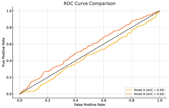
Figure 1.
ROC curves of baseline models. Doted line shows the chance level.

Table 1.
Selected performance metrics for top stacking models.
In addition to discrimination, we evaluated probability calibration. Figure 2 presents the calibration curves comparing predicted default probabilities with the observed frequencies. The results indicate that while baseline models deviate from perfect calibration, the optimized stacking models reported in Table 1 achieve considerably better alignment between predicted and actual outcomes, as reflected by their low log loss and Brier score values.

Figure 2.
Calibration curves of baseline vs. stacking models.
3.1. Stacking Model Architecture, MLR
The implemented stacking model architecture uses the predictions from multiple domain-specific models—risks, delinquency, payments, spends, and balances—as input features for a logistic regression meta-model. Each stacking configuration is evaluated by combining one prediction from each module, resulting in a diverse set of model ensembles. The performance of each stacked model was assessed using a comprehensive suite of metrics, including the Gini coefficient, ROC AUC, PR AUC, log loss, Brier score, and KS statistic, on both training and test datasets.
The results, summarized in Table 1, demonstrate that the stacking approach achieves exceptionally high discriminatory power, with test Gini coefficients consistently above 0.90 and ROC AUC values exceeding 0.95. The top-performing models exhibit negligible overfitting, as indicated by extremely small relative differences between train and test Gini coefficients (often less than 0.01%). Furthermore, the log loss and Brier scores remain low, and the KS statistic values are robust, underscoring the reliability and calibration of the stacked models. All leading models successfully converged, reflecting numerical stability and the appropriateness of the logistic regression meta-model for this ensemble task.
It should be noted that Figure 1 presents ROC curves of early-stage baseline models for illustrative purposes, which explains the relatively low AUC values shown there. Table 1, on the other hand, reports the results of the final converged stacking models after full optimization and feature selection. These optimized models demonstrate substantially higher ROC AUC values (greater than 0.95), consistent with their overall strong performance across multiple evaluation metrics.
Table 1 presents the performance of the top stacking models, where predictions from multiple domain-specific modules (risks, delinquency, payments, spends, and balances) are combined into a meta-model. The Gini coefficients (both train and test) are consistently around 0.90, which indicates outstanding discriminatory power in distinguishing default from non-default borrowers. The ROC AUC values exceed 0.95, reinforcing the robustness of classification performance. Both the log loss and Brier score are very low, showing that the predicted probabilities are well calibrated and close to observed outcomes. The KS statistic values (≈0.78) confirm strong separation between defaulters and non-defaulters, a benchmark widely used in credit risk modeling. Finally, the Relative Gini Gap between training and testing sets is nearly zero (<0.01%), demonstrating minimal overfitting and excellent generalization. Overall, the results highlight the stacking architecture’s ability to integrate diverse feature modules into a highly accurate and stable predictive model.
The discrimination and calibration performance of the optimized stacking ensemble are visualized in Figure 3, Figure 4, Figure 5 and Figure 6. Figure 3 shows the Receiver Operating Characteristic (ROC) curves for the training and test datasets, confirming excellent generalization with nearly identical AUC values (∼0.95). Figure 4 presents the calibration plots that compare predicted and observed default probabilities, demonstrating the improved probability calibration of the optimized stacking models relative to the baseline logistic regressions. Figure 5 illustrates the discrimination performance across modular stacking configurations using ROC and precision–recall characteristics, further confirming high predictive capability (AUC > 0.95). Finally, Figure 6 depicts the overall architecture of the modular stacking framework, where outputs from the domain-specific modules (risks, delinquency, payments, spends, and balances) are combined through a logistic regression meta-model into a unified and interpretable credit scoring ensemble.
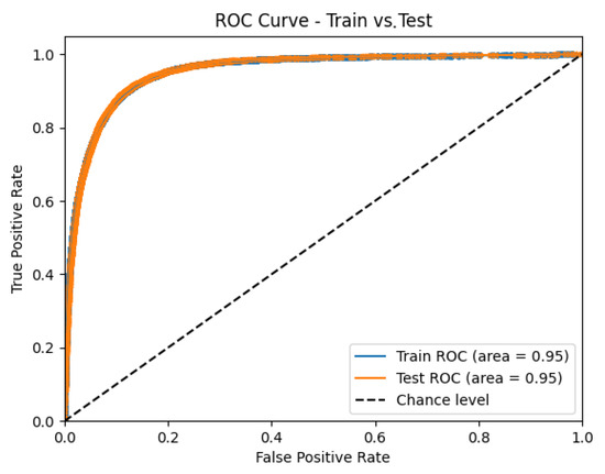
Figure 3.
Receiver Operating Characteristic (ROC) curves for training and test datasets of the optimized stacking model.
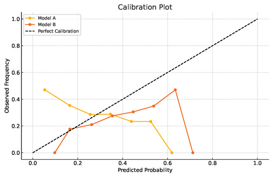
Figure 4.
Calibration curves of optimized stacking models vs. baseline models. This figure compares predicted default probabilities with observed frequencies, illustrating the superior probability calibration achieved by the optimized stacking ensemble relative to baseline logistic regression models.
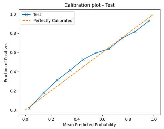
Figure 5.
Discrimination performance of modular stacking models. The figure presents ROC or precision–recall characteristics of the best-performing stacking architectures that integrate domain-specific sub-models (risks, delinquency, payments, spends, and balances). High AUC values (>0.95) confirm outstanding discriminatory capability.
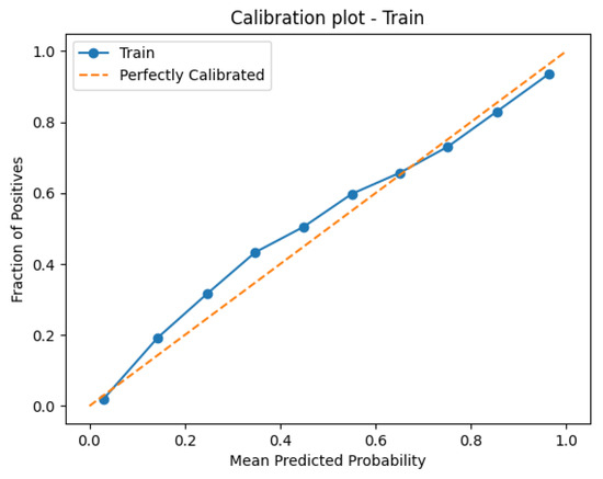
Figure 6.
Architecture of the modular stacking framework for credit scoring. This schematic shows how predictions from individual domain modules are aggregated through a logistic regression meta-model, forming an interpretable yet highly accurate ensemble for heterogeneous borrower data.
The principal strengths of this stacking approach are its flexibility and performance. By allowing the meta-model to learn optimal weights for each module’s prediction, the architecture captures complementary information and mitigates the weaknesses of individual models. The consistently high test Gini and ROC AUC values, together with minimal overfitting, indicate that the stacking ensemble generalizes well and is not unduly influenced by noise or idiosyncrasies in the training data. The interpretability of logistic regression coefficients provides insight into the relative importance of each module’s prediction in the final ensemble.
There are a number of limitations, however, that should be recognized. There is a high computational cost (while training) since to evaluate all module predictions (i.e., all possible combinations), many meta-models have to be trained. The stacking strategy further requires the base models to be diverse; when the base predictions are very close, the gain of stacking is likely to be limited. In addition, although the meta-model is interpretable, the ensemble itself is interpretable as the straightforward individual model prediction as we have more base models. Finally, high performance on the output sets points to the potential information leakage or over-optimistic validation when stacking is not properly cross-validated and correctly detached from the base model training. Further practical notes on training time and scalability are provided in Appendix A.1.
So, the stacking model design provides a flexible and strong concept for blending disparate predictors, attaining state-of-the-art discrimination and calibration. The merits include its flexibility, generalization ability, and interpretability, as well as some demerits of high computational cost, easily being overfitted, and information leakage.
3.2. Hierarchical Multi-Model Logistic Regression Approach
A hierarchical multi-stage logistic regression method was developed to systematically evaluate the predictive performance of various combinations of domain-specific feature modules. Each model architecture was constructed by sequentially incorporating predictions from previous stages as features into subsequent logistic regressions, thereby enabling the assessment of both direct and indirect predictive contributions of each module. The approach resulted in a large ensemble of models, each trained and validated on stratified datasets, with performance metrics including the Gini coefficient, ROC AUC, PR AUC, log loss, Brier score, and KS statistic for both training and test sets.
The results, as illustrated in Table 2, demonstrate that the best-performing models achieve high Gini coefficients (typically above 0.8 on the test set), with minimal overfitting, as evidenced by small gaps between training and test metrics. Notably, models incorporating delinquency and spends modules in early stages consistently outperformed those relying solely on less predictive modules such as risks or payments. The top models also exhibited strong convergence and stability, with no significant degradation in performance when evaluated on unseen data.
Table 2.
Example performance metrics of top converged models.
Table 2 reports the performance of the best converged hierarchical logistic regression models using different feature module combinations. The Gini coefficients (train/test) measure the discriminatory power of the models, with values around 0.80 indicating strong ability to distinguish between default and non-default cases. The log loss and Brier score reflect calibration quality: lower values suggest that predicted probabilities are well aligned with observed outcomes. The KS statistic (Kolmogorov–Smirnov) captures the maximum separation between the cumulative distributions of defaults and non-defaults, with values above 0.70 considered strong in credit scoring practice. Finally, the (test–train)/train (%) column shows the relative gap between training and test Gini values, which remains very small (0.62%), indicating minimal overfitting and good generalization. Together, these results show that the selected models are both accurate and stable, with delinquency and spending features consistently appearing among the most predictive modules.
The main advantages of this method are its flexibility and interpretability. By progressively predicting missing values at each stage, the model can obtain complex, multi-level interactions among different features while preserving the interpretability and elegance of logistic regression. The hierarchical nature also makes it possible to determine which of the most predictive modules and the best sequence of those can provide useful information for feature engineering and model construction. In addition, the method achieves consistent convergence and high test performance over diverse model architectures, indicating that it is robust and widely applicable.
Nevertheless, there are some limitations to be considered. It is computationally costly to train and evaluate a large number of model variants, and this is exacerbated for layers and stages. Focusing on linear logistic regression may also curtail the ability of the model to account for the highly nonlinear nature of interactions and is likely to let some predictiveness be unaccounted for. Moreover, a risk of information leakage is posed by using the stage-wise predictions as features without proper treatment, and the selection of best feature sequences may be dataset- and problem-dependent. Last but not least, even though the optimum models work well, the improvement is marginal as more complex combinations are taught, which indicates the importance of careful selection of models and potential regularization.
To conclude, the hierarchical multi-model logistic regression strategy is a flexible and interpretable process for both the feature and model selection and can achieve high discrimination and good stability. However we stress that its computational cost, linearity assumptions, and information leak risk must be taken into account when upscaling to more data and dimensions.
3.3. Ensemble Architectures with Mean and Median Aggregation
This study evaluated two ensemble architectures—mean and median aggregation—to combine thresholded binary predictions from multiple domain-specific models (risks, delinquency, payments, spends, and balances). Both methods apply thresholds (0.3–0.75) to individual model outputs, then compute either the mean or median across predictions to generate a final ensemble score. The results demonstrate strong performance for both approaches, with test Gini coefficients frequently exceeding 0.80, ROC AUC values above 0.95, and minimal overfitting (relative Gini gaps <1%). For instance, at a threshold of 0.5, median aggregation achieved a test Gini of 0.81 and log loss of 0.29, while mean aggregation produced comparable results (e.g., Gini 0.80 and log loss 0.30). The results are shown in Table 3.
Table 3.
Example performance metrics by aggregation method.
While median aggregation excels in outlier resistance, mean aggregation better captures consensus but is vulnerable to extreme predictions. Both architectures offer practical, interpretable solutions for combining heterogeneous models but may underperform compared to advanced methods like stacking, which optimize model weights. Strengths and limitations of median and mean ensemble methods are shown in Table 4. Future work could explore adaptive thresholding or hybrid approaches to balance robustness and sensitivity.
Table 4.
Strengths and limitations of median and mean ensemble methods.
3.4. Multi-Model Logistic Regression Approach
To compare prediction performance across different types of features, we fit a large collection of logistic regression models, each using some subset of predictions from the risks, delinquency, payments, spends, and balance modules. The Gini coefficient was employed as the principal measure of discrimination, and the models were tested on training and test sets. These results are summarized in Table 5, and the best models (i.e., those achieving the highest Gini on the training set) were trained with Gini coefficients ∼0.81 on the training data (0.80 for the test set) and with all models converging. The subset generation methods rank very well, with the relative difference between test and train Gini always lower than 0.3% for the top models and hence very good generalization beyond the train Gini and very limited over-fitting.
Table 5.
Top 5 models in multi-model logistic regression approach.
The strengths of this approach lie in its flexibility and robustness. By systematically evaluating all meaningful combinations of model predictions, the analysis identifies which modules and their respective models contribute most to predictive power. The consistently high Gini coefficients and low train–test gaps demonstrate that the models are both accurate and generalizable. Also, the logistic regression framework ensures interpretability, allowing for clear attribution of predictive performance to specific input modules.
However, several limitations must be acknowledged. First, the approach is computationally intensive due to the exponential growth in the number of possible model combinations as more modules and models are included. Second, while convergence was achieved for all models, the reliance on linear relationships may limit the ability to capture complex, nonlinear interactions among features. Third, the use of stacked model predictions as features introduces the risk of information leakage if not properly cross-validated. Finally, the marginal improvement in Gini coefficients with increasingly complex combinations suggests diminishing returns, highlighting the need for careful model selection and potential regularization.
Ultimately, the multi-model logistic regression strategy provides a powerful and interpretable framework for feature and model selection, yielding high discrimination with minimal overfitting. Nevertheless, its computational cost and reliance on linearity should be considered when scaling to even larger or more complex modeling tasks.
3.5. Feature Union LR Model
The logistic regression model was constructed using a comprehensive feature set derived from multiple data modules, including balances, spends, payments, delinquency, and risks. The model achieved strong discriminative performance, as evidenced by high training and test set metrics: the Gini coefficient was approximately 0.857 for both train and test sets, while the ROC AUC scores were consistently above 0.928. Precision–recall performance was robust, with PR AUC values around 0.796. The Kolmogorov–Smirnov (KS) statistic exceeded 0.72, indicating excellent separation between positive and negative classes. However, the model failed to converge according to the maximum likelihood estimation routine, which may indicate issues with numerical stability or the presence of highly correlated or extreme predictors. Results are shown in Table 6.
Table 6.
Performance metrics on training and test sets.
Despite these successes, the model has some weaknesses. Non-convergence of an optimization algorithm may be due to an overparameterized model or a set of data with collinear features, which interfere with the validity of coefficient estimates and interpretations. The use of a high number of features (approximately 189 predictors) compared to the number of observations could also lead to overfitting; however, the good concordance between train and test metrics gives some security with respect to generalizability. Moreover, logistic regression is reliable and interpretable, but it assumes a linear relationship between the log odds of the outcome and the predictors, and this may not be the case in practice. The accuracy of the model also may be restricted because it employs imputed data, which may bias the results if the process that caused those data to be missing is not completely understood or not properly controlled for.
On the other hand, the advantages of the model are that it is somewhat transparent and easy to interpret, enabling easy evaluation of the importance of parameters and diagnostics of the model. Fairly high and stable performance scores over training and testing sets suggest that the model is learning useful structures from the data and is not seriously overfitting. Logistic regression also enables domain knowledge to be included and hypothesis testing when the assumption of no confounding is violated (i.e., non-additive effects), which is particularly relevant in applications where interpretation and model validation are preferred to accurate prediction.
Overall, aspects in which the logistic regression model excels include strong predictive performance, and interpretability; limitations, including the chance of non-convergence, collinearity, and overfitting, should be weighed carefully. In the future, it could consider feature selection, regularizations, or different model architectures to control these points and further improve the reliability of this model.
4. Discussion
4.1. Comparative Analysis of Model Architectures
This section presents a comprehensive comparison of the model architectures evaluated in this study: single logistic regression, multi-model logistic regression with feature subsets, hierarchical/multi-stage logistic regression, ensemble with median, ensemble with mean, and stacking (meta-learning). Each architecture is analyzed with respect to its mathematical foundation, practical implementation, predictive performance, robustness, interpretability, and computational demands. The discussion is structured to highlight both the strengths and limitations of each approach, providing insights for model selection and future research.
4.1.1. Single Logistic Regression
A single logistic regression model is trained on the complete set of features from all modules.
The model estimates the probability of the target class given features x as:
where is the learned coefficients.
This model (single logistic regression model) has pros and cons shown in Table 7.
Table 7.
Pros and cons of logistic regression.
Single logistic regression is suitable for initial exploration and as a baseline, but it may lack the flexibility to capture complex patterns or interactions present in the data.
4.1.2. Multi-Model Logistic Regression with Feature Subsets
In this setting, each logistic regression model is constructed in the same way as described previously, but instead of using the entire feature space X, the model is restricted to a selected subset of features . Each subset S represents a coherent behavioral module, such as delinquency, spending, payments, balances, or risks. This allows us to analyze the predictive contribution of different types of customer information in isolation.
Formally, for a given subset S, the probability of default is estimated as
where is the vector of features belonging to module S, and is the parameters estimated for that module-specific model.
The motivation for this design is twofold. First, it improves interpretability since we can directly assess the relative importance of delinquency-related features versus spending or balance-related features. Second, it mitigates the effects of collinearity that often arise when the entire feature space is used in a single regression. Although each subset model captures only partial information, they serve as essential building blocks for more advanced architectures (e.g., hierarchical models or stacking ensembles), where their outputs are combined.
In practice, we find that the subset models reveal distinct predictive patterns. For example, delinquency-related models generally achieve high discriminatory power, while balance-related models contribute stability to long-term forecasts. By comparing their individual performance, we gain insights into which behavioral dimensions are most informative for default prediction.
Multiple logistic regression models have pros and cons demonstrated in Table 8.
Table 8.
Pros and cons of feature module evaluation.
This approach (multiple logistic regression models) is valuable for feature selection and understanding module importance, but it does not use the full potential of inter-module synergies.
4.1.3. Hierarchical Logistic Regression
Predictions from one logistic regression model (stage) are used as features in the next, iteratively building up predictive signals.
At stage k, the model is
where is the prediction from the previous stage. Equation (4) describes the standard logistic regression formulation, where the weighted sum of input features is transformed through a logistic (sigmoid) function. Physically, this means that each customer attribute contributes linearly to a latent risk score, which is then mapped into a probability of default between 0 and 1. Positive coefficients indicate that larger feature values increase risk, while negative coefficients decrease risk, making this formulation directly interpretable in financial terms. More details on hierarchical learning models and their pros and cons can be found in Table 9.
Table 9.
Pros and cons of hierarchical learning models.
Hierarchical models are theoretically appealing for complex, structured data but require careful design and validation to avoid pitfalls such as error propagation.
4.1.4. Ensemble with Median Aggregation
Binary predictions (after thresholding) from multiple models are aggregated by taking the median as
where is the binary prediction from model i.
Median aggregation is robust and simple but may underperform if some models are significantly better than others or if nuanced probability information is important (Check Table 10 for more details).
Table 10.
Pros and cons of median-based ensemble methods.
4.1.5. Ensemble with Mean Aggregation
Binary predictions (after thresholding) from multiple models are aggregated by taking the mean.
where —models predictions, from which mean is taken.
Mean aggregation is smoother and more representative of model consensus but is less robust to outliers and may still underutilize the predictive power of superior models (Table 11).
Table 11.
Pros and cons of mean-based ensemble methods.
4.1.6. Stacking
Predictions from multiple models are used as features for a logistic regression meta-model, which learns optimal combination weights.
where h is the vector of predictions from base models. Equation (7) extends the logistic regression principle to the stacking framework. Here, instead of raw features, the inputs are probability estimates from several base models, each trained on a different subset of behavioral information. Physically, this represents a weighted combination of “expert opinions,” where each base model specializes in one aspect of customer behavior. The meta-model learns how to integrate these signals into a final default probability, providing a more robust and accurate risk assessment. Check Table 12 for more details.
Table 12.
Pros and cons of stacked ensemble methods.
Stacking is theoretically optimal for combining heterogeneous models but requires more data and computational resources. It is best suited for settings where predictive performance is major and interpretability is less critical. An illustrative example of meta-model coefficients and their interpretability is summarized in Appendix A.2.
4.2. Comparative Summary Table
This section provides a comparative analysis of various modeling approaches based on key evaluation dimensions: predictive power, robustness, computational efficiency, interpretability, and flexibility. Each method—ranging from simple logistic regression to more advanced ensemble and hierarchical models—exhibits distinct strengths and limitations. While stacking and hierarchical models typically offer superior predictive accuracy and flexibility, they come at the cost of increased computational demands and reduced interpretability. In contrast, median- and mean-based ensembles prioritize robustness and simplicity, whereas logistic regression serves as a transparent and efficient baseline. The following breakdown highlights how each method performs across these critical dimensions, guiding the selection of an appropriate modeling strategy based on task-specific priorities.
It should be noted that the single logistic regression results reported in Table 3 correspond to a baseline model trained on the entire set of features simultaneously. This approach is sensitive to multicollinearity and overfitting, and as a result it produces weaker indicators compared to the modular logistic regression models reported earlier in Table 3, where features were grouped and optimized within behavioral modules. The discrepancy highlights the advantage of modular decomposition for improving both stability and predictive power.
One can conclude the following results from Table 13:
- Predictive Power: Stacking and hierarchical models generally achieve the highest predictive performance as they can learn complex interactions and optimal combinations of base models. Ensemble methods (mean and median) are robust but may underperform if base models are not equally informative. Single logistic regression provides a reliable baseline but may lack the flexibility to capture complex patterns.
- Robustness: Ensemble with median is the most robust to outliers and noise. Ensemble with mean is less robust but smoother. Stacking and hierarchical models are less robust if base models are highly correlated or if the meta-model overfits.
- Computational Efficiency: Single logistic regression and ensemble methods are computationally efficient. Stacking and hierarchical models are more demanding due to additional training steps.
- Interpretability: Single logistic regression and ensemble methods are highly interpretable. Stacking and hierarchical models are less interpretable due to their complexity.
- Flexibility: Stacking and hierarchical models are the most flexible, capable of capturing complex patterns and interactions. Ensemble methods are less flexible but more robust and easier to implement.
Table 13.
Performance indicators of the baseline single logistic regression trained on the full feature set. Compared to the module-specific models in Table 6, this baseline suffers from multicollinearity and noise, which explains its lower predictive performance.
Table 13.
Performance indicators of the baseline single logistic regression trained on the full feature set. Compared to the module-specific models in Table 6, this baseline suffers from multicollinearity and noise, which explains its lower predictive performance.
| Architecture | Predictive Power | Robustness | Computational Cost | Interpretability | Flexibility | Key Limitation(s) |
|---|---|---|---|---|---|---|
| Single Logistic Regression | Moderate | Low | Low | High | Low | Overfitting, linearity assumption |
| Multi-Model Logistic Regression | Moderate | Moderate | Moderate | High | Moderate | No inter-module interaction |
| Hierarchical/ Multi-Stage Logistic | High | Moderate | High | Moderate | High | Error propagation, complexity |
| Ensemble with Median | Moderate | High | Low | High | Low | Loss of probabilistic info |
| Ensemble with Mean | Moderate | Moderate | Low | High | Low | Sensitive to outliers |
| Stacking (Meta-Learning) | High | High | High | High | High | Overfitting, complexity |
Note: Cell colors indicate qualitative levels: Green = High, Yellow = Moderate, Red = Low.
5. Practical Recommendations
From a practical perspective, the choice of model should balance predictive performance, interpretability, and computational cost. Based on our results, we recommend the following:
- Single logistic regression is appropriate when interpretability is the primary requirement, computational resources are limited, or when models must be deployed in highly constrained environments.
- Modular logistic regression offers a middle ground, allowing interpretability at the module level (delinquency, balances, etc.) while delivering stronger performance and stability than a single model.
- Stacking ensembles should be chosen when the marginal gain in accuracy and robustness is critical, such as in large-scale credit portfolios where even small improvements in prediction translate to substantial financial impact. However, they come with higher computational and maintenance costs.
To make these trade-offs clearer, Figure 7 presents a decision flowchart illustrating when stacking provides sufficient added value to justify its complexity.
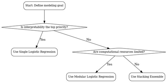
Figure 7.
Decision flowchart for selecting between single, modular, and stacking models based on interpretability, resource constraints, and accuracy requirements.
6. Conclusions
This paper introduces a modular credit scoring framework designed to accommodate heterogeneous borrower data while preserving interpretability and regulatory compliance. Through the use of Weight of Evidence (WoE) transformations and logistic regression-based sub-models, we developed and evaluated a series of model architectures—ranging from stacking ensembles to hierarchical regressions—tailored to real-world financial datasets. Our empirical results show that modular structures can achieve high levels of predictive accuracy and robustness, often matching or exceeding baseline logistic regression models, particularly in scenarios where missing or partial data is prevalent.
Importantly, the architecture allows for localized model retraining, which significantly reduces maintenance costs and enhances operational flexibility. While the performance metrics are encouraging, the computational cost and risk of information leakage in complex ensembles require careful attention. Future work should consider integrating monotonic constraints, exploring Bayesian model averaging, and extending the approach to multi-class credit risk settings. Overall, this research contributes to the ongoing dialogue between regulatory transparency and algorithmic performance in financial risk modeling.
The key takeaway is that modular decomposition combined with stacking represents a practical compromise between interpretability and predictive accuracy. For financial institutions, this framework offers both high-performing default prediction and transparency in understanding how different behavioral modules contribute to risk. Future work may extend this modular stacking design to other financial datasets or to non-logistic meta-learners, further exploring the balance between interpretability and accuracy.
Author Contributions
Conceptualization, A.A.S.; methodology, A.A.S.; software, A.A.S.; validation, all authors; formal analysis, A.A.S.; investigation, A.A.S.; writing—original draft preparation, all authors; writing—review and editing, all authors; visualization, all authors; supervision, M.R.B.; project administration, M.R.B. All authors have read and agreed to the published version of the manuscript.
Funding
This research received no external funding.
Institutional Review Board Statement
Not applicable.
Informed Consent Statement
Not applicable.
Data Availability Statement
The datasets presented in this article are not readily available because the data are part of an ongoing work. Requests to access the datasets should be directed to corresponding author.
Acknowledgments
We thank Innopolis University for generously funding this endeavor.
Conflicts of Interest
The authors declare no conflicts of interest.
Appendix A. Computational Considerations and Meta-Model Interpretability
Appendix A.1. Computational Cost and Scalability
The computational requirements of the proposed modular stacking framework primarily arise from the independent training of base models and the subsequent meta-model fitting. Each module (risks, payments, delinquency, spends, and balances) was trained and validated separately, enabling efficient parallelization. On a standard workstation (Intel Core i9 CPU, 32 GB RAM), the complete training of all module ensembles required approximately 20–25 min, including cross-validation and meta-model optimization.
Since modules are independent, the computational cost scales linearly with the number of sub-models, allowing for straightforward horizontal scaling in production environments. In practical financial systems where modular risk components are often maintained separately, this design offers a natural pathway toward incremental retraining and low-latency model deployment.
Appendix A.2. Meta-Model Interpretability
The stacking meta-model employs a logistic regression layer that linearly combines the probability outputs of domain-specific sub-models. Each coefficient in this meta-layer directly represents the relative contribution of the corresponding domain module to the overall credit scoring decision.
Table A1 provides an illustrative example of how the meta-model’s coefficients can be interpreted. Positive coefficients indicate higher contribution to the predicted probability of default, while negative coefficients correspond to mitigating effects.
Table A1.
Illustrative interpretation of meta-model coefficients. Positive coefficients indicate stronger contributions to predicted default risk.
Table A1.
Illustrative interpretation of meta-model coefficients. Positive coefficients indicate stronger contributions to predicted default risk.
| Domain Module | Meta-Model Coefficient | Interpretation |
|---|---|---|
| Risk Indicators | +1.22 | Strong positive contribution to default risk |
| Payment History | +0.87 | Moderate positive impact |
| Balance Utilization | –0.34 | Slightly lowers predicted default probability |
| Delinquency Profile | +0.65 | Positive association with risk |
| Spending Behavior | –0.15 | Weak stabilizing effect |
This hierarchical structure preserves feature-level interpretability within each module (via logistic regression coefficients and WoE transformations) while maintaining transparency at the meta-level. Consequently, the full pipeline remains auditable and explainable in line with regulatory expectations for credit scoring models.
References
- Appiahene, P., Missah, Y. M., & Najim, U. (2020). Predicting bank operational efficiency using machine learning algorithm: Comparative study of decision tree, random forest, and neural networks. Advances in Fuzzy Systems, 2020(1), 8581202. [Google Scholar] [CrossRef]
- Ben-Gal, I. (2008). Bayesian networks. In Encyclopedia of statistics in quality and reliability. Wiley. [Google Scholar] [CrossRef]
- Cutler, A., Cutler, D. R., & Stevens, J. R. (2012). Random forests. In Ensemble machine learning: Methods and applications (pp. 157–175). Springer. [Google Scholar] [CrossRef]
- Fidrmuc, J., & Lind, R. (2020). Macroeconomic impact of Basel III: Evidence from a meta-analysis. Journal of Banking & Finance, 112, 105359. [Google Scholar] [CrossRef]
- Hastie, T. J. (2017). Generalized additive models. In Statistical Models in S (pp. 249–307). Routledge. [Google Scholar] [CrossRef]
- Kaggle. (2022). American express-default prediction. Available online: https://www.kaggle.com/competitions/amex-default-prediction/data (accessed on 3 June 2025).
- Lee, G. H. (2008). Rule-based and case-based reasoning approach for internal audit of bank. Knowledge-Based Systems, 21(2), 140–147. [Google Scholar] [CrossRef]
- Mahadevan, A., & Mathioudakis, M. (2023). Cost-effective retraining of machine learning models. arXiv, arXiv:2310.04216. [Google Scholar] [CrossRef]
- Martens, D., Baesens, B., Van Gestel, T., & Vanthienen, J. (2007). Comprehensible credit scoring models using rule extraction from support vector machines. European Journal of Operational Research, 183(3), 1466–1476. [Google Scholar] [CrossRef]
- Olaniran, O. R., Sikiru, A. O., Allohibi, J., Alharbi, A. A., & Alharbi, N. M. (2025). Hybrid random feature selection and recurrent neural network for diabetes prediction. Mathematics, 13(4), 628. [Google Scholar] [CrossRef]
- Scheres, S. H. (2010). Classification of structural heterogeneity by maximum-likelihood methods. In Methods in enzymology (Vol. 482, pp. 295–320). Elsevier. [Google Scholar]
- Tarka, P. (2018). An overview of structural equation modeling: Its beginnings, historical development, usefulness and controversies in the social sciences. Quality & Quantity, 52, 313–354. [Google Scholar]
- U.S. Department of Housing and Urban Development. (2009). Fair lending: A guide for housing counselors. Available online: https://www.hud.gov/sites/documents/fair_lending_guide.pdf (accessed on 3 June 2025).
- Van Ginkel, J. R., Linting, M., Rippe, R. C., & Van Der Voort, A. (2020). Rebutting existing misconceptions about multiple imputation as a method for handling missing data. Journal of Personality Assessment, 102(3), 297–308. [Google Scholar] [CrossRef] [PubMed]
- West, D. (2000). Neural network credit scoring models. Computers & Operations Research, 27(11–12), 1131–1152. [Google Scholar] [CrossRef]
Disclaimer/Publisher’s Note: The statements, opinions and data contained in all publications are solely those of the individual author(s) and contributor(s) and not of MDPI and/or the editor(s). MDPI and/or the editor(s) disclaim responsibility for any injury to people or property resulting from any ideas, methods, instructions or products referred to in the content. |
© 2025 by the authors. Licensee MDPI, Basel, Switzerland. This article is an open access article distributed under the terms and conditions of the Creative Commons Attribution (CC BY) license (https://creativecommons.org/licenses/by/4.0/).