Abstract
Statistical factor models are widely applied across various domains of the financial industry, including risk management, portfolio selection, and statistical arbitrage strategies. However, conventional factor models often rely on unrealistic assumptions and fail to account for the fact that financial markets operate under multiple regimes. In this paper, we propose a regime-switching factor model estimated via a particle filtering algorithm, which is a Monte Carlo-based method well-suited for handling nonlinear and non-Gaussian systems. Our empirical results show that incorporating dynamic structure and a regime-switching mechanism significantly enhances the model’s ability to detect structure breaks and adapt to evolving market conditions. This leads to improved performance and reduced drawdowns in the equity statistical arbitrage strategies.
1. Introduction
Factor analysis plays a critical role in quantitative finance, with applications in asset pricing, risk management, portfolio selection, and statistical arbitrage strategies. Broadly speaking, factor models can be categorized into two types: explicit factor models, which fall under supervised learning, and statistical factor models, which are typically unsupervised. Compared to explicit factor models such as Barra risk model (Barra, 2004), statistical factor models offer two key advantages: they are numerically more stable in capturing the underlying covariance structure using fewer factors, and they are asset-class agnostic, making them broadly applicable across different markets.
However, financial markets are far from stationary. They undergo regime shifts that fundamentally alter market dynamics. For example, the transition from the unusually low-volatility environment of 2017 to the volatility spike in February 2018, the U.S. Federal Reserve’s abrupt rate hikes in 2022, or geopolitical shocks such as Russia’s invasion of Ukraine all represent regime-switching events. Standard statistical factor models, which assume globally static factor loadings, often fail to forecast covariances accurately during such transitions, the very moments when robust risk modeling is most needed.
The literature on statistical factor models has evolved to address such challenges. Early PCA-based factor models (Jolliffe, 2004) are limited in parametric structure and perform poorly when within group variation dominates between group variation (Hinton & Dayan, 1997; McLachlan & Peel, 2000). In the 1980s, maximum likelihood (ML) factor analysis estimated via the EM algorithm was introduced by (Rubin & Thayer, 1982). This was further generalized in the 1990s by (Ghahramani & Hinton, 1996), who proposed the mixture of factor analyzers (MFA). By combining clustering with local dimension reduction, MFA works better than classical ML factor analysis due to its ability of segmenting data into different market regimes, each with its own factor structure, improving on the “one-size-fits-all” ML factor models.
Despite these advancements, within each regime, MFA still uses a classical ML factor model which assumes i.i.d. hidden factors and Gaussian innovations. Dynamic factor models extend this framework by introducing a recursive structure for hidden factor returns, capturing their time dynamics more realistically. Earlier works such as (Bai & Wang, 2014; Forni et al., 2009; Geweke & Zhou, 1996; Kim & Halbert, 1999) typically assume a simple first-order autoregressive (AR(1)) structure for factor returns, while later developments extend the underlying process to ARMA and VARMA formulations (see Peña & Poncela, 2004, 2006; Urteaga et al., 2017; Varga & Szendrei, 2024). These dynamic factor models are capable of handling both stationary and nonstationary hidden factors.
In this paper, we focus on the AR(1)-based dynamic factor models with regime-switching factor loadings governed by a first order Markov chain. Such models, or, more generally, regime switching state space models, have been extensively studied in the literature (see Carvalho et al., 2010; Kim & Halbert, 1999; Whiteley et al., 2010). This framework not only models the hidden factor process but also captures the regime switching effects inherent in financial data. Common estimation approaches include Gibbs sampling, the EM algorithm, particle MCMC and particle filtering. We adopt the particle filtering framework for its computational efficiency and sequential structure, which aligns closely with real world trading scenarios.
Particle filtering (Arulampalam et al., 2002; Doucet & Johansen, 2009) is a class of Monte Carlo methods designed to perform recursive Bayesian inference when analytical solutions such as the Kalman filter or Baum–Welch algorithm are infeasible. Although it is well developed when model parameter values are known, parameter learning in more complex settings remains challenging. Specifically, when parameters evolve according to a stochastic process rather than being constant, such as in applications in finance, an adaptive parameter learning algorithm becomes critical. To learn the parameter values, one early approach by (Liu & West, 2001) incorporates parameters into the hidden state vector, but this often exacerbates the degeneracy issue in particle filtering. More computationally robust approaches have been introduced in (Djuric et al., 2012) and (Carvalho et al., 2010). Instead of combining parameter estimation to the learning algorithm they marginalize over parameters to reduce the estimation variance of their system. In this work, we implemented a particle filtering algorithm inspired by (Djuric et al., 2012) and (Carvalho et al., 2010) and applied it to estimate a regime switching dynamic factor model using real financial data.
The goal of this study is not merely methodological. By evaluating statistical factor models in the context of statistical arbitrage strategies, we directly test their practical usefulness for risk modeling. Following (Avellaneda & Lee, 2010), we adopt a simplified trading framework where performance differences are driven primarily by the quality of covariance forecasts. In this setup, a superior factor model should deliver more accurate residuals, adapt more quickly to regime shifts, and ultimately provide a stronger risk foundation for arbitrage strategies.
The rest of paper is organized as follows: Section 2 introduces the state space model and its estimation methods, including Kalman filter, EM algorithm, Particle filter, and the more recent development in parameter learning—the particle learning algorithm. Section 3 presents statistical factor models such as the MLE factor model, mixture of factor analyzers and the regime-switching dynamic factor model. We highlight the evolution of statistical factor models over recent decades and provides a simulation study demonstrating the effectiveness of particle learning algorithm for estimating the regime-switching dynamic factor model. Section 4 presents empirical studies applying the regime-switching dynamic factor model in the context of equity stat-arb strategy and compares its performance to the conventional MLE factor model. Finally, Section 5 concludes the paper.
2. State Space Model and Its Estimation
A state space model is a framework used to describe the evolution of a dynamical system over time, particularly when the system is only partially observed. It has numerous applications in finance, such as time series prediction (alpha generation), statistical factor analysis (risk modeling), and portfolio selection (see Kim & Halbert, 1999; Kolm & Ritter, 2014). In the most general form, a state space model can be represented by the following:
where denotes the hidden states with dimension k, and the observations with dimension s. The terms and represent the noise terms for the evolution Equation and the observation Equation , with dimensions w and v, respectively. Throughout this work, we use bold lowercase to denote vectors, and bold uppercase to denote matrices. The functions and are general nonlinear functions defining the state transition and observation processes. When the parameter values of the above equations are known, inference about the hidden states can be efficiently performed using the recursive Bayesian algorithm (Arulampalam et al., 2002), which is summarized as Algorithm 1:
| Algorithm 1 Recursive Bayesian Algorithm |
|
Where the denominator in Equation is called the marginal likelihood (or evidence), which is another intergral needs to be solved (see Appendix A).
2.1. Kalman Filter and EM-Algorithm Estimation
When the dynamical system described by Equations and is linear, time-invariant, and finite-dimensional, functions , and can be expressed in the following form:
and if we further assume , , then the well-known Kalman filter can be derived to solve Equations and analytically as described in (Arulampalam et al., 2002) and in Algorithm A1 (see Appendix B). When parameters , are unknown, the EM algorithm (Ghahramani & Hinton, 1996) can be employed for their estimation. In this framework, the Kalman filter is used in the E-step to compute the expected sufficient statistics of the hidden states, while the M-step updates the parameter estimates (see Appendix C).
2.2. Particle Filter
When the dynamical system and do not admit a linear-Gaussian representation as in and , deriving an analytical solution for the recursive Bayesian inference becomes challenging. In such cases, particle filtering techniques has been a very popular approach for solving nonlinear dynamical system, including models like the stochastic volatility model (See Djuric et al., 2012).
The Sequential Importance Sampling (SIS) filter (Gordon et al., 1993) approximates the joint posterior density at time t using the importance sampling method:
where is the Dirac delta function, and is the importance weight for particle i, given by the following:
With the factorization
sequential sampling of states becomes feasible, which forms the foundation of SIS particle filter (see Algorithm A4).
In practice, the SIS particle filter suffers from weight degeneracy: the variance of the weight will increase over time until only one particle dominates. To alleviate this issue, the Sequential Importance Resampling (SIR) filter resamples the particles based on their weights, replicating those particles with large weights and eliminating particles with small weights, thereby reducing variance (Doucet & Johansen, 2009).
Although the optimal importance density for a generic particle filter algorithm is (Doucet et al., 2000), the SIR particle filter typically uses as an important density and applies resampling at each step (see Algorithm A5). While SIR filter improves stability, it still has weaknesses (Pitt & Shephard, 1999). First, if there is an outlier at time t, the weights will be unevenly distributed and the filter will become imprecise. Second, the predictive density often fails to capture tail behavior accurately, causing some particles to drift into low-likelihood regions during step 2 in Algorithm A5.
To address these limitations, the auxiliary particle filter proposed by (Pitt & Shephard, 1999) introduces a lookahead step—also known as the auxiliary variable mechanism. This approach uses a predictive weighting scheme (see Algorithm A6 step 1) that estimates the likelihood of the upcoming observation given the predicted state, a process often referred to as lookahead weighting. When the observation equation is informative in a dynamical system, the auxiliary particle filter usually will reduce variance in particle weights and hence perform better.
2.3. Particle Filter with Parameter Learning
The particle filter algorithms discussed so far assume that model parameters are known. However, in many applications, model parameters are typically unknown. Learning the static parameter values—or more broadly—identifying the coefficient evolution process—is a critical aspect of system identification. The integration of parameter learning into the particle filtering framework has been extensively studied (Kantas et al., 2015).
One idea is to treat parameters as additional hidden state variables in the particle filtering framework, but this approach often leads to severe degeneracy issue. To address this issue, Liu and West (2001) proposed introducing an artificial evolutional model for the parameters and augment the hidden state space by including them.
Another idea is to integrate out (or marginalize out) the parameters whenever feasible (Djuric et al., 2012; Schon et al., 2005; Storvik, 2002). The benefits of the marginalized particle filter have been discussed in (Özkan et al., 2013).
Building on these ideas, Carvalho et al. (Carvalho et al., 2010) introduced particle learning approach, a novel particle filter with the embedded parameter learning step. The particle learning method marginalizes both the parameters and the hidden states by only tracking their sufficient statistics, which are updated later using recursive Bayesian algorithm and Kalman filter, respectively. It is also constructed under the auxiliary particle filter framework; the performance improvement has been demonstrated in (Carvalho et al., 2010; Lopes & Tsay, 2010).
In our paper, we develop a simplified version of the particle learning algorithm to estimate regime-switching dynamic factor model.
2.3.1. Particle Learning
Particle learning algorithm was introduced by Carvalho et al. in (Carvalho et al., 2010), extending the idea of auxiliary particle filter to incorporate parameter learning. While the overall filtering scheme is the same as auxiliary particle filter, the key innovation lies in tracking the “essential state” .
Specifically, includes the following:
- the sufficient statistics of the parameter vector ;
- the sufficient statistics of hidden states , ; and
- the current value of the parameter vector, ;
The reason we include parameter value in the essential state is because for evaluating likelihood and drawing samples from predictive density we need to use parameter values. However, their values are not directly sampled at each step, which most likely causes degeneracy issues; instead, they are inferred offline from their associated sufficient statistics. This approach is also referred to as marginalization by simulation.
The derivation of this filter starts with the recursive relation:
where
and
So, given the particles of , we can construct a Monte Carlo estimate for by sampling from and , respectively. After that we can update and deterministically. The particle learning method can be summarized as Algorithm 2:
| Algorithm 2 Particle Learning |
|
Where denotes the deterministic updating function for parameter sufficient statistics and denotes Kalman filter for state sufficient statistics update.
3. Statistical Factor Analysis
Statistical factor analysis is a technique used to explain the correlation structure of multivariate observations through a lower-dimensional set of unobserved factors. The model can be expressed as follows:
where is vector of observations, is vector of statistical factors, and is factor loading matrix. is the error term that follows certain distribution assumption. The hidden factors are often assumed to follow an i.i.d. standard normal distribution, i.e., , and are assumed to be independent of the error term .
3.1. MLE Factor Analysis
The most commonly used approach for estimating the factor model in Equation is the Expectation-Maximization (EM) algorithm for maximum likelihood estimation (MLE) (Ghahramani & Hinton, 1996; McLachlan & Peel, 2000; Rubin & Thayer, 1982). The EM algorithm for the maximum likelihood estimation of the factor model is outlined below as Algorithm 3:
| Algorithm 3 EM algorithm for Statistical Factor Analysis |
|
The EM algorithm starts with certain initial values for and and terminates when the rate of change in the log likelihood falls below some critical value. The log likelihood can be computed as follows:
3.2. Mixture of Factor Analyzer
The factor model in Equation is a global linear model. However, in many real world applications—such as in financial engineering—it fails to reflect the fact that the observed data present multiple regimes whose behaviors differ materially. To address this limitation, the mixture of factor analyzer (MFA) model extends the MLE statistical factor model by combining local dimension reduction method with a Gaussian mixture model for clustering. Specifically, the MFA model can be described in the following form:
where , and the index i denotes the component (or regime), drawn from a categorical distribution with mixing probabilities . is the factor loading matrix specific to component i. Following the formulation in (Ghahramani & Hinton, 1996), we assume the observation covariance for each component are the same, and the number of mixture is fixed prior to the estimation step. The EM algorithm for estimating the parameters of the MFA model is described below in Algorithm 4:
| Algorithm 4 EM algorithm for Mixture of Factor Analyzer |
|
Starting with initial values of for , , and , we can iterate Algorithm 4 until convergence. The log-likelihood of the observed data under the MFA model is given by the following:
where denotes the set of all model parameters.
3.3. Regime-Switching Dynamic Factor Model
Although the mixture of factor analyzer (MFA) model can capture data generated from multiple regimes, it still assumes the observations are i.i.d. and fails to account for the temporal persistence of market regimes. In practice, particularly in financial applications, market regimes tend to persist over time, with each regime exhibiting distinct statistical properties. Regime switching model equipped with Markov chain mechanism can better model the regime persistence and capture the abrupt regime shifts more efficiently than commonly used “low-pass filtering” approaches such as rolling window estimation. It fits better for financial time series, where capturing time dynamics is essential.
3.3.1. Methods
In this work, we represent the regime-switching dynamic factor model within a state space framework. The estimation of regime switching state space models has been well studied in the literature (Andrieu et al., 2010; Carter & Kohn, 1994; Kim & Halbert, 1999), with most approaches relying on the Markov Chain Monte Carlo (MCMC) algorithms. MCMC approaches are not only computationally very expensive, but also suffer slow convergence issue. Moreover, they are batch (offline) algorithms in nature which limits their use in real-time trading.
In this work, we will rely on the particle learning technique that is introduced in Section 2.3.1 as our estimation method. Computationally, it is significantly faster than MCMC algorithms and, being an online algorithm, it can be adopted in the real time trading environment. The convergence of particle filtering algorithm is well studied in the literature (Del Moral, 2004; Doucet et al., 2000).
Another key advantage of the particle filtering framework is its modular design, which makes it highly adaptable to complex model structures. Additional structure can be incorporated into the system relatively easier than MCMC framework, as long as it remains possible to draw samples from the importance density and evaluate the likelihood function upon receiving the new observations (see Djuric et al., 2012; Urteaga et al., 2017 for examples).
To introduce our model, we first define a discrete latent regime variable which captures the regime at time t. The essential state used in the particle learning algorithm is then extended as follows:
where and denote the sufficient statistics for the parameters and the hidden states, respectively, and denotes the model parameters.
The model is specified as follows:
where denotes the inverse Gamma distribution , . In this representation, we model heavy tailed innovation using the data augmentation scheme of (Carlin & Polson, 1991), where at each time t, we will follow the two step approach: (i) , (ii) , so that where is a diagonal matrix.
If the degree of freedom is given, then at each time step t, our system is a conditionally Gaussian model. To derive the particle learning algorithm for this model (Equations (24)–(26)), we compute the predictive density by integrating out the latent regime variable :
where is the conditional likelihood, which is derived in Appendix G, and is given by the estimated transition matrix. To propagate , we sample from the posterior distribution:
The particle filtering algorithm for regime switching dynamic factor model is described below in Algorithm 5:
| Algorithm 5 Particle Filter for Regime Switching Dynamic Factor Model |
|
Where the deterministic updating formula in step 5 is given by the following:
where . The sampling density in step 4 is derived in Appendix H. As discussed in Appendix G, we can assume each row of transition matrix , , follows a Dirichlet distribution , for , and their sufficient statistics can be updated as follows:
For step 6, following the spirit of (Djuric et al., 2012), we compute parameter values directly from their sufficient statistics rather than sampling them. Compared with the particle learning method of (Carvalho et al., 2010), which samples parameter values from their posterior distributions, our analytical solution reduces Monte Carlo variance and improves computational efficiency without sacrificing model fidelity. Specifically, the parameter updates are as follows:
Here, we use the posterior mode (MAP) as a transition probability estimate. In this step, denotes the Kalman filter update, and the detailed recursion is presented in Algorithm A1 of Appendix B. We also extend Carvalho’s approach by incorporating a mixture of Gaussian innovations, which provides a closer alignment with the heavy-tailed and non-Gaussian features observed in empirical financial data.
3.3.2. Simulation Analysis
To validate our particle filtering estimation algorithm, we apply it to a controlled synthetic data environment. We generate synthetic scenarios based on a three-regime dynamic factor model involving 15 synthetic instruments. This setup allows us to test the algorithm’s ability to recover latent states and parameters under regime-switching dynamics in a controlled setting.
The “true” model parameters are specified as follows:
Factor loading matrices ():
The observation covariance matrices ():
The state transition matrix ():
and the regime transition matrix is as follows:
Since factor loadings and factor returns are not separately identifiable within our model structure, our validation analysis focuses on three key aspects:
- Regime detection: assessing whether the algorithm can correctly identify latent regime shifts (see Figure 1);
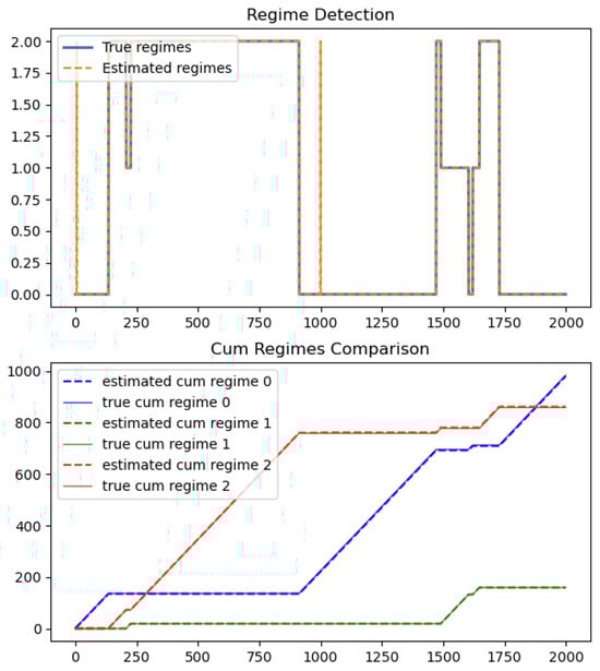 Figure 1. Regime detection.
 - Idiosyncratic risk estimation: evaluating the accuracy of instrument-specific variance estimates (see Figure 2);
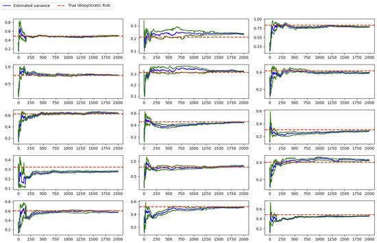 Figure 2. Idiosyncratic Risk Estimation.
 - Cumulative expected returns’ tracking: examining how well the estimated expected returns align with the “true” cumulative return over time (see Figure 3).
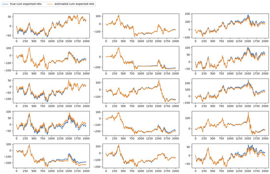 Figure 3. Cumulative expected return tracking.
To initialize the particle filtering algorithm, we begin with non-informative priors. For example, the mean of the factor loading matrix is set to a zero rectangular matrix under each regime
The prior left covariance of the loading matrix is initialized with high dispersion, specifically a diagonal matrix whose entries are set to 10, to ensure weak prior information and allow the data to drive the estimation. The same applies to the prior distribution chosen for the factor transition matrix , and the idiosyncratic risk distribution, . In each case, we begin with non-informative means and large prior dispersion, thereby minimizing prior influence and ensuring that the posterior estimates are predominantly shaped by the data.
As the following results demonstrate, even when initialized with non-informative priors, our algorithm converges accurately to the “true” parameters, thereby validating the effectiveness of Algorithm 5.
As shown in Figure 1, the algorithm accurately captures the evolution of hidden regimes from both regime detection plot and cumulative regimes comparison plot.
In terms of idiosyncratic risk (or error variance), the algorithm also converges to their unbiased estimates, as illustrated in Figure 2. The blue line represents the mean of the particle estimates, while the green lines denote the 25th and 75th quantiles.
The most critical metric in statistical factor analysis is the model’s ability to accurately track expected returns. In our synthetic experiments, the proposed model exhibits strong performance in the cumulative expected return, as illustrated in Figure 3.
4. Results in Statistical Arbitrage Strategy
In both academic and industry, equity statistical arbitrage strategy (equity stat-arb) usually means the idea of trading groups of stocks against either explicit or synthetic factors, which can be seen as the generalization of “pairs-trading” (see Avellaneda & Lee, 2010). In some cases, we would long an individual stock and short the factors, and in others we would short the stock and long the factors. Overall, due to the netting of long and short positions, our exposure to the factors will be small. One key step of the equity stat-arb strategy is the decomposition of assets’ returns into the systematic part and idiosyncratic part. When we use a more effective factor model, we can have a better decomposition and hence a better strategy performance.
4.1. Market Neutral Strategy
In this paper, we evaluate the quality of factor models within the context of an equity statistical arbitrage strategy. Inspired by the approach of (Khandani & Lo, 2008), in order to avoid the unnecessary complexity of signal generation and potential overfitting issues, we adopt a deliberately simple reversion signal which is the negative value of previous day’s residuals. To ensure market neutrality, we construct a dollar-neutral portfolio each day, with equal dollar amounts allocated to long and short positions.
To be specific, we compare the performance of trading strategies derived from both the regime-switching dynamic factor model and static MLE factor model. For estimating the regime-switching dynamic factor model, we employ Algorithm 5. The initialization follows the same procedure as in the simulation analysis (Section 3.3.2), with one refinement: to improve initial convergence, we use the estimates from a mixture of factor analyzer (MFA), trained on a “burn-in” sample from 3 January 2005 to 1 January 2011, as the initial mean of the factor loadings, . Furthermore, the residualization step is implemented in a rolling window framework so that the residuals are always generated out-of-sample. For the estimation of the static MLE factor model, we employed Algorithm 3 as described in Section 3.1. This serves as our baseline approach, providing a standard maximum likelihood estimation of factor loadings and covariances under the assumption of a single, time-invariant regime.
For computational efficiency, we designed a relatively lean experiment by restricting the dataset to the daily prices of the Dow Jones 30 constituents. Since factor models do not require the same scale-invariance adjustments as PCA-based approaches, we use raw returns rather than normalized return for the estimation. In this setting, we employ a three-factor model and assume that the factor loadings evolve according to a two-regime Markov chain. For each experiment, we use rolling window walk forward time series cross-validation framework to run our backtesting. The training data sample size is 120 days (around 6 months) and the test data sample size is 5 days (around one week). The objective of this experiment is not to identify or interpret the economic meaning of market regimes. Instead, our goal is to demonstrate that when a regime shift occurs, regardless of its underlying cause, our system adapts more rapidly to the new distribution (or data-generating process). This adaptability enables it to deliver a superior risk model for statistical arbitrage strategies.
After the residualization step, we can generate our signals using a naive rule-based approach. If the previous day’s residual for asset i has , where d is the threshold, then we will say that the asset i is over-priced at time and short this asset for the next time stamp t. For , we will perform the opposite operation. For simplicity, in our experiment, we set . At each time step, we form a dollar-neutral portfolio by applying the mean-variance closed form solution to both the long and short sides:
where is the covariance matrix of returns, represents the rule-based prediction, and is a scaling factor that controls overall risk.
4.2. Performance Comparison
We run this naive strategy using the MLE static factor model, the dynamic factor model without regime switching mechanism, and the regime switching dynamic factor model, respectively, and the strategy performance is as shown in Figure 4:
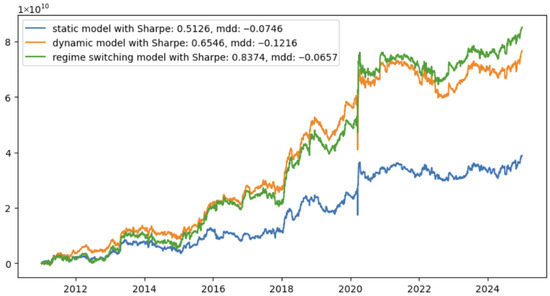
Figure 4.
Equity stat-arb performance comparison.
We can see from Figure 4 that the strategy achieves a higher Sharpe ratio and a lower maximum drawdown when using the regime-switching dynamic factor model compared to both the static MLE factor model and the simple dynamic factor model. Specifically, the improvement in Sharpe is approximately 63%, while the reduction in maximum drawdown is about 12%. We also observe that the simple dynamic factor model performs well, telling us the importance of modeling the dynamics of factor returns in equity arbitrage strategies. However, incorporating the regime-switching mechanism provides an additional advantage: it meaningfully reduces drawdowns during market regime shifts (most notably during the COVID period) and improves estimation accuracy in the aftermath of such events. Based on these findings, we conclude that dynamic factor models consistently outperform static factor models, and that incorporating a regime-switching mechanism enables the model to adapt much more quickly to abrupt regime shifts, such as those observed during COVID, than conventional approaches.
The associated historical effective sample size plot and regime detection plot are given in Figure 5:
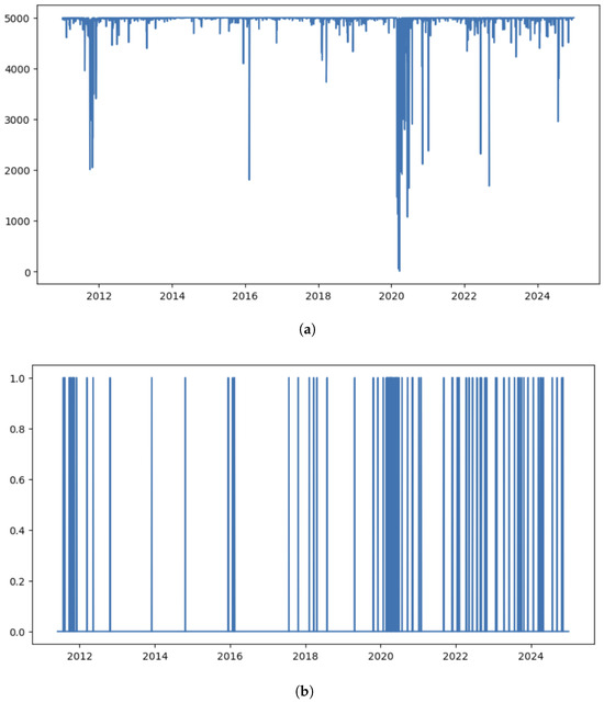
Figure 5.
(a) Effective sample size at each day when running particle filter. (b) Regime detection when using regime switching particle filter.
In the above graphs, the effective sample size (ESS) is used to measure the stability of particle filtering algorithm in real data, and defined as:
where are normalized weights.
From the ESS graph, we observe that the particle filter estimation is stable, as most of the time the ESS is larger than 2000 for a three-factor model. From the regimes detection, we can see there are more regime changes in the 2020 COVID period and early 2024. Indeed our regime switching model performs better during those periods compared with the simple dynamic factor model and static factor model.
It is also worth noting that although our model does not assume the factor return process is stationary, it is also informative to check the estimated transition matrix:
The modulus of its eigenvalues are: 0.074, 0.046, 0.046. Since , the implied factor dynamics are stationary.
Although determining the number of factors and regimes is beyond the scope of this work, it is still worthwhile to examine results under varying specifications. By checking different numbers of factors and regimes, we can assess whether our earlier findings remain robust across alternative setups. The relevant results are summarized in the Table 1 and Table 2 as follows:

Table 1.
Sharpe ratio across alternative setups.
Table 2.
Maximum drawdown across alternative setups.
From the results above, we observe that our findings remain consistent across varying specifications of factor numbers and regime counts. This robustness test provides further confidence that improvements from regime-switching dynamic factor model are not sensitive to any specific parameter choices.
5. Discussion
This paper investigates the estimation of a regime-switching dynamic factor model using a particle learning algorithm. Through simulation studies, we validate our estimation approach by evaluating regime detection accuracy, idiosyncratic risk estimation, and the model’s ability to track expected returns. The empirical study in the equity statistical arbitrage framework further demonstrates that the regime-switching dynamic factor model outperforms a conventional static MLE factor model in capturing underlying data dynamics.
The particle learning algorithm implemented in this paper builds on the framework of (Carvalho et al., 2010), with several modifications. First, we extend the innovation distribution to a mixture of Gaussian distributions. Second, we simplify the parameter learning step by only tracking the sufficient statistics, rather than using the marginalization via simulation. Lastly, we apply the estimated model to the empirical data and compare its performance against the conventional MLE factor model.
We are able to see the performance improvements in the equity statistical arbitrage strategy when using our model. Our model not only improves the Sharpe ratio but also minimizes the maximum drawdown. These results align with our initial motivation: It is well known that financial market operates under multiple regimes, and incorporating the regime switching mechanism that is governed by the hidden Markov model in our model representation allows us better model the structural shifts and enhances risk management—particularly during periods of elevated volatility and contagion risk.
While the current particle learning algorithm is based on the vanilla auxiliary particle filter, there remains a lot of room to improve the quality of our particle filtering algorithm and hence improve the tracking of hidden states (or hidden factors in this model). For instance, the ABC-based sequential Monte Carlo filter (Jasra et al., 2010) could further enhance the filtering accuracy. Additionally, incorporating more robust, heavy-tailed innovation distributions (Schoutens, 2005) may improve the robustness of our estimation, particularly in the presence of extreme market movements. Investigating more sophisticated specifications for the hidden factor process, including nonstationary factor models, would also be a promising direction for future research (Peña & Poncela, 2004, 2006).
Author Contributions
Conseptualization, Y.M. and R.J.F.; methodology, Y.M. and R.J.F.; software, Y.M.; validation, Y.M. and R.J.F.; formal analysis, Y.M.; investigation, Y.M. and R.J.F.; resources, Y.M.; data curation, Y.M.; writing—original draft preparation, Y.M.; writing—review and editing, Y.M.; visualization, Y.M.; supervision, R.J.F.; project administration, R.J.F.; funding acquisition, Y.M. All authors have read and agreed to the published version of the manuscript.
Funding
This work was supported and funded by the Strategic Partnership for Industrial Resurgence (SPIR) program at Stony Brook University.
Institutional Review Board Statement
Not applicable.
Informed Consent Statement
Not applicable.
Data Availability Statement
All data used in this study are publicly available from the yfinance API: https://ranaroussi.github.io/yfinance/index.html, accessed on 20 July 2025.
Conflicts of Interest
The authors declare no conflict of interest.
Appendix A. Marginal Likelihood
The marginal likelihood can be represented by the following:
Appendix B. Kalman Filter and Smoother
| Algorithm A1 Kalman Filter |
|
Where is the Kalman gain and can be computed by the following:
When estimating hidden states in offline mode (i.e., when the full time series data is available) or when performing the EM algorithm to estimate model parameters, the Kalman smoother is typically used to refine those state estimates using future observations as well (see Algorithm A2).
| Algorithm A2 Kalman Smoother |
Where is the Kalman smoothing gain.
Appendix C. EM-Algorithm for State Space Model Estimation
| Algorithm A3 EM algorithm |
|
Where , will be estimated by the Kalman filter and smoother. can be updated by backward recursions:
which is initialized by .
Appendix D. SIS Particle Filter
| Algorithm A4 SIS Particle Filter |
|
Appendix E. SIR Particle Filter
| Algorithm A5 SIR Particle Filter |
|
Appendix F. Auxiliary Particle Filter
| Algorithm A6 Auxiliary Particle Filter |
|
Appendix G. Probability Density Function of
The likelihood function is straightforward to derive. Given , and the equation , the likelihood function follows the normal distribution , where
Appendix H. Probability Density Function of p(xt | xt−1, θt−1, yt)
Based on Bayes’ rule, we can factor as:
Expressing quadratic form to normal form:
where . If we let , , then
where . Hence,
Appendix I. Conjugate Prior of Categorical Distribution
The Dirichlet distribution, which is a multivariate generalization of the Beta distribution, is usually used as the conjugate prior distribution of the categorical distribution (also known as multinomial distribution) (See Murphy, 2014). The probability density function of the Dirichlet distribution is defined as:
where lives in a K () dimensional probability simplex with constraints , and . is called concentration parameters with constraint . Assume we have a set of data generated from Categorical distribution with parameters , and . Then we can represent likelihood as:
where , and is the Dirac Delta function. Since the parameter vector also lives in a K dimensional probability simplex, and the Dirichlet distribution belongs to exponential family, so it becomes a natural choice of conjugate prior for parameter . If we assume prior distribution for as:
Hence, the posterior is also Dirichlet:
In other words, the posterior sufficient statistics can be updated by simply adding the empirical counts . It is easy to show the posterior mode (MAP estimate) is given by:
where , . At the meanwhile, the posterior mean is given by:
References
- Andrieu, C., Doucet, A., & Holenstein, R. (2010). Particle markov chain monte carlo methods. Journal of the Royal Statistical Society Series B: Statistical Methodology, 72, 269–342. [Google Scholar] [CrossRef]
- Arulampalam, M., Maskell, S., Gordon, N., & Clapp, T. (2002). A tutorial on particle filters for online nonlinear/non-Gaussian Bayesian tracking. IEEE Transactions on Signal Processing, 50, 174–188. [Google Scholar] [CrossRef]
- Avellaneda, M., & Lee, J. H. (2010). Statistical arbitrage in the US equities market. Quantitative Finance, 10, 761–782. [Google Scholar] [CrossRef]
- Bai, J., & Wang, P. (2014). Identification and bayesian estimation of dynamic factor models. Journal of Business & Economic Statistics, 33, 221–240. [Google Scholar] [CrossRef]
- Barra. (2004). Barra risk model handbook. MSCI. [Google Scholar]
- Carlin, B. P., & Polson, N. G. (1991). Inference for nonconjugate Bayesian models using the Gibbs sampler. Canadian Journal of Statistics, 19, 399–405. [Google Scholar] [CrossRef]
- Carter, C. K., & Kohn, R. (1994). On Gibbs sampling for state space models. Biometrika, 81, 541–553. [Google Scholar] [CrossRef]
- Carvalho, C. M., Johannes, M. S., & Lopes, H. F. (2010). Particle learning and smoothing. Statistical Science, 25, 88–106. [Google Scholar] [CrossRef]
- Del Moral, P. (2004). Feynman-kac formulae: Genealogical and interacting particle systems with applications. Springer. [Google Scholar]
- Djuric, P. M., Khan, M., & Johnston, D. E. (2012). Particle filtering of stochastic volatility modeled with leverage. IEEE Journal of Selected Topics in Signal Processing, 6, 327–336. [Google Scholar] [CrossRef]
- Doucet, A., Godsill, S., & Andrieu, C. (2000). On sequential Monte Carlo sampling methods for Bayesian filtering. Statistics and Computing, 10, 197–208. [Google Scholar] [CrossRef]
- Doucet, A., & Johansen, A. M. (2009). A tutorial on particle filtering and smoothing: Fifteen years later. Oxford Handbook of Nonlinear Filtering, 12, 656–704. [Google Scholar]
- Forni, M., Giannone, D., Lippi, M., & Reichlin, L. (2009). Opening the black box: Structure factor models with large cross sections. Econometric Theory, 25(5), 1319–1347. [Google Scholar] [CrossRef]
- Geweke, J., & Zhou, G. (1996). Measuring the price of the arbitrage pricing theory. The Review of Financial Studies, 9(2), 557–587. [Google Scholar] [CrossRef]
- Ghahramani, Z., & Hinton, G. E. (1996). Parameter estimation for linear dynamical systems (Technical report CRG-TR-96-2). University of Toronto, Department of Computer Science.
- Gordon, N., Salmond, D., & Smith, A. (1993). Novel approach to nonlinear/non-Gaussian Bayesian state estimation. IEE Proceedings F Radar and Signal Processing, 140, 107. [Google Scholar] [CrossRef]
- Hinton, G. E., & Dayan, P. (1997). Modeling the manifolds of images of handwritten digits. IEEE Transactions on Neural Networks, 8, 65–74. [Google Scholar] [CrossRef] [PubMed]
- Jasra, A., Singh, S. S., Martin, J. S., & McCoy, E. (2010). Filtering via approximate Bayesian computation. Statistics and Computing, 22, 1223–1237. [Google Scholar] [CrossRef]
- Jolliffe, I. T. (2004). Principal component analysis. Springer. [Google Scholar]
- Kantas, N., Doucet, A., Singh, S. S., Maciejowski, J., & Chopin, N. (2015). On particle methods for parameter estimation in state-space models. Statistical Science, 30, 328–351. [Google Scholar] [CrossRef]
- Khandani, A. E., & Lo, A. W. (2008). What happened to the quants in August 2007? Evidence from factors and transactions data. Journal of Financial Markets, 14, 1–46. [Google Scholar] [CrossRef]
- Kim, C. J., & Halbert, D. C. R. (1999). State-space models with regime switching: Classical and Gibbs-sampling approaches with applications. The MIT Press. [Google Scholar]
- Kolm, P. N., & Ritter, G. (2014). Multiperiod portfolio selection and Bayesian dynamic models. Risk, 28(3), 50–54. [Google Scholar] [CrossRef]
- Liu, J., & West, M. (2001). Combined parameter and state estimation in simulation-based filtering. In Sequential monte carlo methods in practice (pp. 197–223). Springer. [Google Scholar]
- Lopes, H. F., & Tsay, R. S. (2010). Particle filters and Bayesian inference in financial econometics. Journal of Forecasting, 30, 168–209. [Google Scholar] [CrossRef]
- McLachlan, G., & Peel, D. (2000). Finite mixture models. Wiley. [Google Scholar]
- Murphy, K. P. (2014). Machine learning: A probabilistic perspective. MIT Press. [Google Scholar]
- Özkan, E., Šmïdl, V., Saha, S., Lundquist, C., & Gustafsson, F. (2013). Marginalized adaptive particle filtering for nonlinear models with unknown time-varying noise parameters. Automatica, 49, 1566–1575. [Google Scholar] [CrossRef]
- Peña, D., & Poncela, P. (2004). Forecasting with nonstationary dynamic factor models. Journal of Econometrics, 119, 291–321. [Google Scholar] [CrossRef]
- Peña, D., & Poncela, P. (2006). Nonstationary dynamic factor analysis. Journal of Statistical Planning and Inference, 136, 1237–1257. [Google Scholar] [CrossRef]
- Pitt, M. K., & Shephard, N. (1999). Filering via simulation: Auxiliary particle filters. Journal of the American Statistical Association, 94, 590–599. [Google Scholar] [CrossRef]
- Rubin, D. B., & Thayer, D. T. (1982). EM algorithms for ML factor analysis. Psychometrika, 47, 69–76. [Google Scholar] [CrossRef]
- Schon, T., Gustafsson, F., & Nordlund, P. J. (2005). Marginalized particle filters for mixed linear/nonlinear state-space models. IEEE Transactions on Signal Processing, 53, 2279–2289. [Google Scholar] [CrossRef]
- Schoutens, W. (2005). Lévy processes in finance: Pricing financial derivatives. Wiley. [Google Scholar]
- Storvik, G. (2002). Particle filters for state-space models with the presence of unknown static parameters. IEEE Transactions on Signal Processing, 50, 281–289. [Google Scholar] [CrossRef]
- Urteaga, I., Bugallo, M. F., & Djurić, P. M. (2017). Sequential Monte Carlo for inference of latent ARMA time-series with innovations correlated in time. EURASIP Journal on Advances in Signal Processing, 2017, 84. [Google Scholar] [CrossRef]
- Varga, K., & Szendrei, T. (2024). Non-stationary financial risk factors and macroeconomic vulnerability for the UK. International Review of Financial Analysis, 97(C), 103866. [Google Scholar] [CrossRef]
- Whiteley, N., Andrieu, C., & Doucet, A. (2010). Efficient Bayesian inference for switching state-space models using discrete particle Markov Chain Monte Carlo methods. arXiv, arXiv:1011.2437. [Google Scholar] [CrossRef]
Disclaimer/Publisher’s Note: The statements, opinions and data contained in all publications are solely those of the individual author(s) and contributor(s) and not of MDPI and/or the editor(s). MDPI and/or the editor(s) disclaim responsibility for any injury to people or property resulting from any ideas, methods, instructions or products referred to in the content. |
© 2025 by the authors. Licensee MDPI, Basel, Switzerland. This article is an open access article distributed under the terms and conditions of the Creative Commons Attribution (CC BY) license (https://creativecommons.org/licenses/by/4.0/).