Article

Delineating Housing Submarkets Using Space–Time House Sales Data: Spatially Constrained Data-Driven Approaches

School of Economic, Political and Policy Sciences, The University of Texas at Dallas, Richardson, TX 75080, USA
*
Author to whom correspondence should be addressed.
J. Risk Financial Manag. 2023, 16(6), 291; https://doi.org/10.3390/jrfm16060291
Submission received: 13 April 2023 / Revised: 30 May 2023 / Accepted: 30 May 2023 / Published: 2 June 2023
(This article belongs to the Special Issue Shocks, Public Policies and Housing Markets)

Abstract

:
With the increasing availability of large volumes of space–time house data, delineating space–time housing submarkets is of interest to real estate agents, homebuyers, urban policymakers, and spatial researchers, among others. Appropriately delineated housing submarkets can help nurture submarket monitoring and housing policy developments. Although submarkets are often expected to represent areas with similar houses, neighborhoods, and amenities characteristics, delineating spatially contiguous areas with virtually no fragmented small areas remains challenging. Furthermore, housing submarkets can potentially change over time along with concomitant urban transformations, such as urban sprawl, gentrification, and infrastructure improvements, even in large metropolitan areas, which can complicate delineating submarkets with data for lengthy time periods. This study proposes a new method for integrating a random effects model with spatially constrained data-driven approaches in order to identify stable and reliable space–time housing submarkets, instead of their dynamic changes. This random effects model specification is expected to capture time-invariant spatial patterns, which can help identify stable submarkets over time. It highlights two spatially constrained data-driven approaches, ClustGeo and REDCAP, which perform equally well and produce similar space–time housing submarket structures. This proposed method is utilized for a case study of Franklin County, Ohio, using 19 years of space–time private house transaction data (2001–2019). A comparative analysis using a hedonic model demonstrates that the resulting submarkets generated by the proposed method perform better than popular alternative submarket creators in terms of model performances and house price predictions. Enhanced space–time housing delineation can furnish a way to better understand the sophisticated housing market structures, and to help enhance their modeling and housing policy. This paper contributes to the literature on space–time housing submarket delineations with enhanced approaches to effectively generate spatially constrained housing submarkets using data-driven methods.

1. Introduction

A consensus opinion expressed in the housing and real estate literature is that heterogeneity in various aspects, including price, exists in urban housing markets. Accordingly, an entire housing market should be divided into several submarkets, or market segments, to improve house price prediction accuracy. For example, Watkins (2001) points out that a housing market can be better analyzed as a set of distinct submarkets instead of one single homogeneous market. Bourassa et al. (2003) conclude that “housing submarkets matter, and location plays the major role in explaining why they matter.” A rich set of literature in the delineation of housing submarkets also reports the importance of location (e.g., Goodman and Thibodeau 1998, 2003; Bourassa et al. 1999; Hwang and Thill 2009; Helbich et al. 2013; Keskin and Watkins 2017). However, most empirically identified submarkets are merely based on one- or two-year pooled housing data, without serious temporal consideration (e.g., Goodman and Thibodeau 2007; Wu and Sharma 2012). Thus, their results may not reflect chronological changes and can be affected by short-term fluctuations. That is, housing submarkets delineated with data for a short time period may not be reliable and consistent over time. This outcome is often attributable to either data availability constraints affiliated with a temporal dimension or the lack of appropriate and robust analytical methods to account for both spatial and temporal information.
The intrinsic significance of recognizing housing submarkets lies in the inherent heterogeneity in prices, internal characteristics, and external locations of houses. Hwang and Thill (2009) expound upon the following four housing submarket natures: substitutability, heterogeneity, durability, and rigidity. Bourassa et al. (1999) and Pryce (2013) define housing submarkets as a group of similar dwellings that are close substitutes for one another within, but relatively poor substitutes of those outside of, their groupings. Following this latter convention, the space–time housing submarkets in this paper have been delimited as space-constrained and time-invariant groups containing similar houses. Space means the identified submarkets are geographically constrained; time denotes the existence of consistent housing patterns over time. Because space–time data are decomposable into systematic space–time trends and small-scale stochastic variations, the focus in this paper is on consistent and reliable space–time housing patterns (i.e., trends) instead of dynamic changes (i.e., variations). Hwang and Thill (2009) contend that housing submarkets, at the macro-level, are durable in the sense that, once built, housing structures and locations are not going to experience dramatic changes on a large scale (i.e., historical inertia prevails) beyond age-sensitive downgrading (e.g., deterioration). Thus, uncovering reliable and stable space–time housing submarkets is vital for policymakers and urban planners when analyzing and addressing urban affairs, such as the internal structure of cities, residential mobility, residential segregation, revitalization effects, and urban development, to name a few possibilities.
Housing submarket delineation has been utilized in various arenas, including strategic housing planning policy (e.g., Jones 2002) and housing price forecasting (e.g., Chen et al. 2009). Whereas housing submarkets can be delineated based on areal units such as census tracts or school districts, use of these units is often criticized because of their ad hoc or subjective nature. Although common clustering methods, such as K-means and hierarchical, have been popularly utilized, each submarket in their delineation results commonly comprises numerous fragmented small areas scattered across a study area. Even employing methods to achieve spatially contiguous housing submarkets does not totally eliminate identifying homogeneous and spatially non-contiguous submarkets (Keskin and Watkins 2017). Furthermore, identification of stable spatial–temporal housing submarkets increases in complexity with the addition of a temporal dimension (e.g., Kopczewska and Ćwiakowski 2021). Addressing this issue, this paper aims to present a novel approach to generate stable space–time housing submarkets. Specifically, the purpose of this paper is twofold. First, to summarize a method combining the random effects (RE) statistical model with spatially constrained data-driven approaches to identify stable space–time housing submarkets from a large volume of spatiotemporal housing data. Second, to investigate different ways of incorporating spatial perspectives into traditional data-driven methods by introducing two spatially constrained data-driven clustering and graph partitioning algorithms, ClustGeo and REDCAP (REgionalization with Dynamically Constrained Agglomerative clustering and Partitioning), in an empirical case study delineating housing submarkets in Franklin County, Ohio (OH).
The rest of this paper is organized as follows. Section 2 presents a literature review about housing submarket delineations and Section 3 discusses the research method for space–time housing submarket delineations. Then, Section 4 describes the study area and the analysis design, and Section 5 presents the analysis results. Finally, Section 6 presents a discussion and conclusions.

2. Literature Review

A very sizeable literature (e.g., Goodman and Thibodeau 1998; Bourassa et al. 1999; 2010; Watkins 2001; Usman et al. 2020) discusses the formulation of housing submarkets that condenses to the following three main analytical frameworks: a priori framework, classical data-driven, and spatially constrained data-driven. Their corresponding results are, respectively, geographic, non-geographic, and spatially constrained submarkets. The primary difference among these three schemes lies in how the construction of housing submarkets treats either locational attributes or their spatial proximity context. This section focuses on these three approaches, further discussing space–time procedures for housing market segmentation.

2.1. Housing Submarket Delimitation Using a Priori Framework

Within a traditional a priori framework, studies about spatial submarkets argue that location, especially its spatial proximity dimension, plays a more important role than the physical housing structures themselves in defining a housing submarket. These investigations delineate spatially contiguous submarkets based upon expert experiences, such as those of real estate agents, or existing administrative boundaries, such as municipal borders, school districts, census tracts, racial neighborhood divisions, and/or land-use zoning borders. For example, Straszheim (1975) combines census tracts on the basis of racial composition to formulate housing submarkets. Mulligan et al. (2002) adopt nine different real estate districts as housing submarkets in their study. Goodman and Thibodeau (1998, 2003) construct spatial submarkets by aggregating spatially adjacent zip code postal zones, census tracts, or census block groups within the same municipality and independent school district to achieve a minimum number of house transactions. The benefits of this framework are that it usually produces meaningful and spatially contiguous local regions for its resulting submarkets and takes advantage of houses or neighborhoods close to each other that share many common public services and locational accessibility to numerous privilege points. Yet, criticism of this category of methods is mainly because (1) delineations based upon expert opinions are subjective and ad hoc—often experts and/or agents cannot unanimously agree; and (2) administrative boundaries may not align with manifestations of the real housing market process and mechanism (Jones et al. 2005)—e.g., homebuyers do not necessarily limit themselves to seeking similar nearby houses, compromising/removing the local exchangeability property of houses from submarkets.

2.2. Housing Submarket Delimitation Using Classical Data-Driven Methodologies

Another alternative framework for determining housing submarkets is based upon classical data-driven statistical methods, such as cluster analysis, classification, or spatial statistical/econometrics techniques. The underlying logic instructs the input of physical/structural house attributes and neighborhood characteristic variables into data-driven algorithms to find close substitutes among houses or geographic areas, enabling a delineation of submarkets, i.e., let the data speak for themselves. Bourassa et al. (1999) apply principal component analysis (PCA) coupled with K-means cluster analysis to group dwellings according to their similar housing and neighborhood features, ultimately constructing pure aspatial housing submarkets. Their results demonstrate that a hedonic price model with submarkets based on statistical routines for Melbourne, Australia, yields a lower weighted mean squared error than its counterpart with spatial submarkets defined by the traditional a priori method. Hwang and Thill (2009) apply the fuzzy c-means clustering method (FCM) to derive housing submarkets in the Buffalo–Niagara Falls metropolitan statistical area (MSA). Kauko (2004) utilizes a self-organizing map (SOM) and learning vector quantification (LVQ), two popular neural network-based techniques, to identify Amsterdam housing market segments. The prominent advantages of this latter framework are that it requires little-to-no prior knowledge and is statistically robust across study areas. Moreover, outcomes from this stratagem are typically objective and achieve a higher degree of internal homogeneity and external heterogeneity for submarkets. Its main potential weakness is that despite the well-known real estate adage that location is so important, the house submarkets derived from data-driven algorithms disregard this important age-old maxim, and, hence, have very spatially fragmented submarket compositions. Therefore, their identified boundaries may not be practically meaningful and/or their resulting housing submarket structures may be difficult to interpret or understand.

2.3. Housing Submarket Delimitation Using Spatially Constrained Data-Driven Approaches

Housing submarket delineations with the two preceding approaches are not without criticism. On the one hand, a priori methods emphasize spatially contiguous and meaningful boundaries. However, their results tend to contain large within-submarket variation. On the other hand, data-driven statistical methods usually demarcate more homogenous housing submarkets than those obtained with the a prior method, but often fail to create spatially contiguous ones. No agreement exists in the academy about the superiority of one strategy over the other. Fortunately, the more recent literature began recognizing the importance of both spatial and aspatial factors in determining housing submarkets. Studies (e.g., Watkins 2001; Bourassa et al. 2003; Helbich et al. 2013; Usman et al. 2020) contend that instead of merely considering the similarity of housing characteristics or geographic contiguity, housing submarkets should be determined simultaneously utilizing both spatial and aspatial factors.
The third framework, spatially constrained data-driven approaches, comes into play to bridge the two aforementioned frameworks and combines their advantages. To achieve spatial proximity in housing submarkets, Bourassa et al. (2010) include geographic coordinates as additional variables in hierarchical clustering. Wu and Sharma (2012) impose spatial constraints in the following way: they use spatially aggregated units (census blocks), and then incorporate relative location (distance to amenities) and absolute location (geographic coordinates of census block centroids) in PCA and cluster analysis. However, these methods treat the geographic location attributes just like other non-spatial attributes. Thus, they lack flexibility to allow differential weightings between spatial and non-spatial attributes. Furthermore, the higher the dimension of input variables, the less weight spatial attributes tend to receive. The case of a relatively large set of non-spatial variables tends to diminish the desired geographic constraint, helping to induce a coterminous outcome.
To remedy these preceding deficiencies, some spatially explicit models or algorithms were developed to impose either soft or hard spatial constraints on the delineation of geographic clusters. For example, Assunção et al. (2006) propose the Spatial Kluster Analysis by Tree Edge Removal (SKATER) algorithm, which several housing submarket papers subsequently adopted to delineate spatially constrained submarkets (Helbich et al. 2013; Soltani et al. 2021). SKATER is a graph partitioning algorithm based upon a minimum spanning tree (MST) that links spatial neighbors with the lowest cost. The clusters (subtrees) partitioned according to this MST are inherently spatially contiguous. Wu et al. (2018) propose the Density-Based Spatial Clustering (DBSC) algorithm, which explicitly considers both spatial proximity and attribute similarity, to identify homogeneous and spatially contiguous housing submarkets in Shenzhen, China. However, their density-based algorithm was originally devised to cluster point data, making it unsuitable for polygon data. Their study demonstrates this latter contention by generating submarkets that remain very fragmented despite the inclusion of spatial constraints. The literature also houses other spatially explicit algorithms, such as ClustGeo and REDCAP (Chavent et al. 2018; Guo 2008), preforming spatial regionalization, but an absence of their applications for housing submarket segmentation persists to this day. This paper innovatively applies these two latter spatially constrained data-driven algorithms to urban housing submarket delineation, filling this literature gap as one of its contributions. In addition, it summarizes a comparative analysis assessment of them.

2.4. Space–Time Housing Submarket Delineations

Despite the current availability of more spatially constrained data-driven algorithms, studies taking into account both spatial proximity and the temporal dimension are scarce in the housing submarkets and real estate literature. Some recent studies (e.g., Cohen et al. 2016; Yuan et al. 2018; Wu et al. 2019; Hu et al. 2020) analyze dynamic house price or housing submarket changes, seeking to explore such influential factors as environmental change, prevailing general economic conditions, intra-urban migration, and urban development or policy change. However, investigations of space–time housing submarket stability are rare. Kopczewska and Ćwiakowski (2021) constitute one exception. They examine whether identified submarkets in each time period are temporally stable or consistent with those identified for another period. In their empirical study of house transaction data in Warsaw, Poland, from 2006 to 2015, they report calculated spatiotemporal varying geographically weighted regression (GWR) coefficients, and then use these quantities as input variables into a K-means clustering technique to delineate housing submarkets, finding that the spatiotemporal stability of their delimitations reaches 80%, as indexed by the Rand and the Jaccard similarity indices. This outcome provides motivation for developing a data-driven analytical tactic to construct stable space–time housing submarkets.

3. Research Method

This section overviews the employed research method for demarcating space–time housing submarkets with two spatially constrained clustering algorithms—REDCAP and ClustGeo—coupled with an RE model. In doing so, the discussion summarizes a hedonic price model comparison and evaluation of the performance of the resulting delineated submarkets.

3.1. Spatially Constrained Clustering Algorithms: REDCAP and ClustGeo

REDCAP combines agglomerative hierarchical clustering with graph partitioning (Guo 2008). This method, an extension of the SKATER algorithm, involves the following two main components: MST generation and MST partitioning. In its step 1, it constructs a connectivity graph of spatial neighbors and, in its step 2, it computes the MST by minimizing the overall cost of the network tree. In its step 3, the MST is partitioned into k-subtrees by recursively selecting k − 1 edges whose removal maximizes the following objective function:
f l = S S D T S S D A + S S D B ,
where l denotes a chosen edge to cut the tree T, A and B denote two trees created by removing edge l from tree T, S S D T is the total sum of the squared deviations for tree T, and S S D A and S S D B are the sums of the squared deviations of trees A and B, respectively. Because optimal graph partitioning is an NP-hard problem, a heuristic is invoked to speed up solving the MST partitioning problem (Assunção et al. 2006).
Guo (2008) recounts a crucial weakness in the SKATER algorithm. He points out that the contiguity matrix is not dynamically updated during the process of constructing an MST and cutting the subtrees. An example involving two spatial objects that are not spatially contiguous in the beginning but become spatial neighbors if later they belong to two clusters that are next to each other, illustrates this shortcoming. Guo adopted the agglomerative clustering method with three different classical linkage criteria (i.e., single-linkage, average-linkage, and complete-linkage) to build the spatially contiguous MST, and then provided two different constraining strategies (first-order and full-order neighbor constraints) to partition a tree to find optimal clusters. In total, Guo presents six contiguity-constrained methods in the REDCAP family with a combination of the three linkage types and the two constraint types. Reapplying this same idea extends this family of possibilities to more methods using other clustering linkages, such as Ward’s minimum variance criterion (i.e., within-submarket similarity is maximized, whereas between-submarket similarity is minimized, on average—an analysis of variance conceptualization). REDCAP is the generalization of the SKATER algorithm and simplifies to SKATER when the first-order neighbor constraint combines with a single-linkage spanning tree.
Chavent et al. (2018) propose ClustGeo, a Ward-like hierarchical clustering algorithm with spatial constraints. It introduces the following two distance matrices as inputs into a hierarchical clustering routine: a non-spatial feature distance matrix denoting attribute dissimilarity ( D 0 ) and a spatial distance matrix indicating geographic or spatial dissimilarity ( D 1 ). This algorithm simultaneously considers spatial and non-spatial distance, with a mixing parameter α 0 , 1 controlling the trade-off between attribute and geographic dissimilarity under the following classical hierarchical clustering framework:
D α = 1 α D 0 + α D 1 .
A crucial facet of this implementation is to establish the optimal weight α by plotting the two normalized dissimilarity distance metrics for the purpose of increasing spatial contiguity without seriously deteriorating attribute feature homogeneity.
After determining α, an agglomerative clustering algorithm utilizes the mixed distance matrix D α to group observations into hierarchical clusters. When α = 0 , this clustering exploits only the non-spatial feature space D 0 ; that is, it is equivalent to a conventional hierarchical clustering procedure. When α = 1 , clustering takes into account only spatial similarity, reducing the aggregation decision-making to a function of spatial means and their accompanying standard distances.

3.2. A Hedonic Price Model with an RE Term

The RE model is widely used in panel data analyses to capture individual-specific unobserved heterogeneity in calculated statistics. Estimation of this constant heterogeneity derives from repeated measures through differencing and isolating time-invariant components in the model. Recent studies, including Chun (2014), An et al. (2015), Hu et al. (2018), and Griffith et al. (2019), show that an RE term estimated with this model represents robust space-specific and time-invariant heterogeneity. In other words, it estimates stable and robust patterns latent in a space–time data series. Its accompanying model specification may be written as
ln Y i t = X i t β + R E i + ε i t , i = 1 , , n ; t = 1 , , T ,
where i denotes the i th areal unit, which are census block groups in the empirical data analysis in the next section ( n = 868 ); t indicates the t th time period, which is a three-month quarter in the ensuing empirical data analysis ( T = 76 ); Y i t is the median house price per square foot for areal unit i at time t ; X i t is a matrix of attribute covariates for areal unit i at time t ; R E i is the RE term for areal unit i that is common for all t , estimated as time-invariant and space-specific heterogeneity; and ε i t is the white noise residual for each observation tagged as areal unit i at time t .
The hedonic house price model is the most popular statistical rendition in the housing literature for estimating and describing residential dwelling prices (Can 1992; Sirmans et al. 2005; Ottensmann et al. 2008; Shimizu et al. 2010; Geng et al. 2015; Xiao 2017). It also furnishes a popular tool to evaluate the quality of identified real estate submarkets. Its goodness-of-fits and prediction errors across several alternative submarkets provide a basis for making illuminating comparisons. Defining submarket binary 0–1 dummy/indicator variables in order to examine impacts of different submarkets, the hedonic model may be re-expressed as follows:
ln Y i t = X i t β x + X s u b β s u b + ε i t ,
where X s u b denotes the collection of submarket dummy variables; and β x and β s u b , respectively, are attribute and dummy covariate regression coefficient parameters to be estimated. Moreover, this model specification motivates an adjudication about the merits of any given demarcation results, rather than merely encouraging a rather simple model goodness-of-fit assessment of them.

4. The Study Area and Analysis Design

An empirical study using 19 years of house transaction data in Franklin County, OH, from 01/01/2001 to 12/31/2019 exemplifies the delineation of coterminous geographic housing submarkets. Franklin County embodies a typical mid-size private residential dwellings market, roughly equivalent to the national average. It exhibits population size stability with an annual growth rate of 1.1% during the period spanned by its empirical data (i.e., 2001–2019)1. These housing data and variables are open records secured from the Franklin County Auditor (see Appendix A). The dataset consists of all residential building transactions with repeat sales records, including all residential building types. The raw data size is 419,099 location and time-encoded observations. Data cleaning2 renders 301,019 records suitable for data analysis purposes. To make house prices comparable over 19 years, transaction prices were inflation-adjusted to the base year of 2001 using the United States (US) Consumer Price Index (CPI) from the US Bureau of Labor Statistics (https://www.bls.gov/cpi/; accessed on 30 May 2023). Franklin County is situated in the center of the Columbus MSA, with nearly 42% of its land covered by the state capital and county seat, namely the City of Columbus. According to the 2020 US Census estimates3, Franklin County has a population of 1,323,807, making it the most populous county in OH.
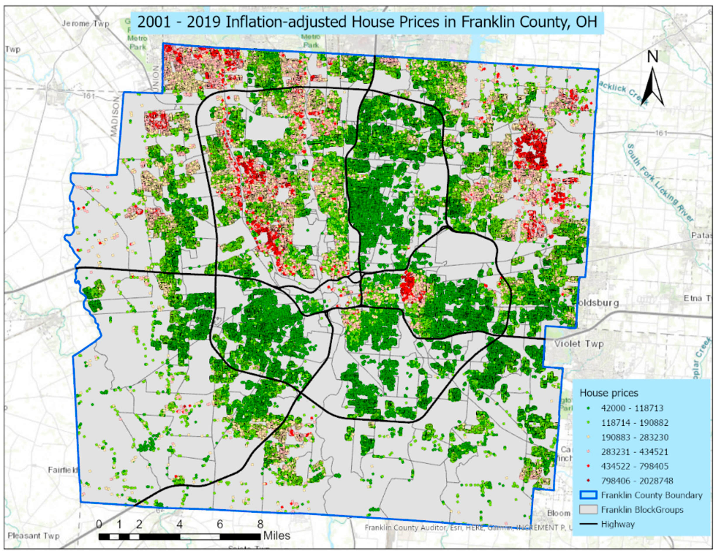
Figure 1 portrays the spatial distribution of inflation-adjusted house prices across Franklin County during the 19 studied years (2001–2019). This map includes the major highway (denoted by black) for reference purposes. House prices have an east–west geographic divider transecting the middle of the county, separating its northern and southern parts: house prices and densities in its north tend to be higher than their counterparts in its south. A prominent positive spatial autocorrelation map pattern is also observable here. More expensive houses, denoted by red or dark red, cluster together, whereas less expensive houses, denoted by green or dark green, spatially concentrate. Or, more generally, houses with similar values (high–high, moderate–moderate, low–low) tend to cluster in geographic space. 
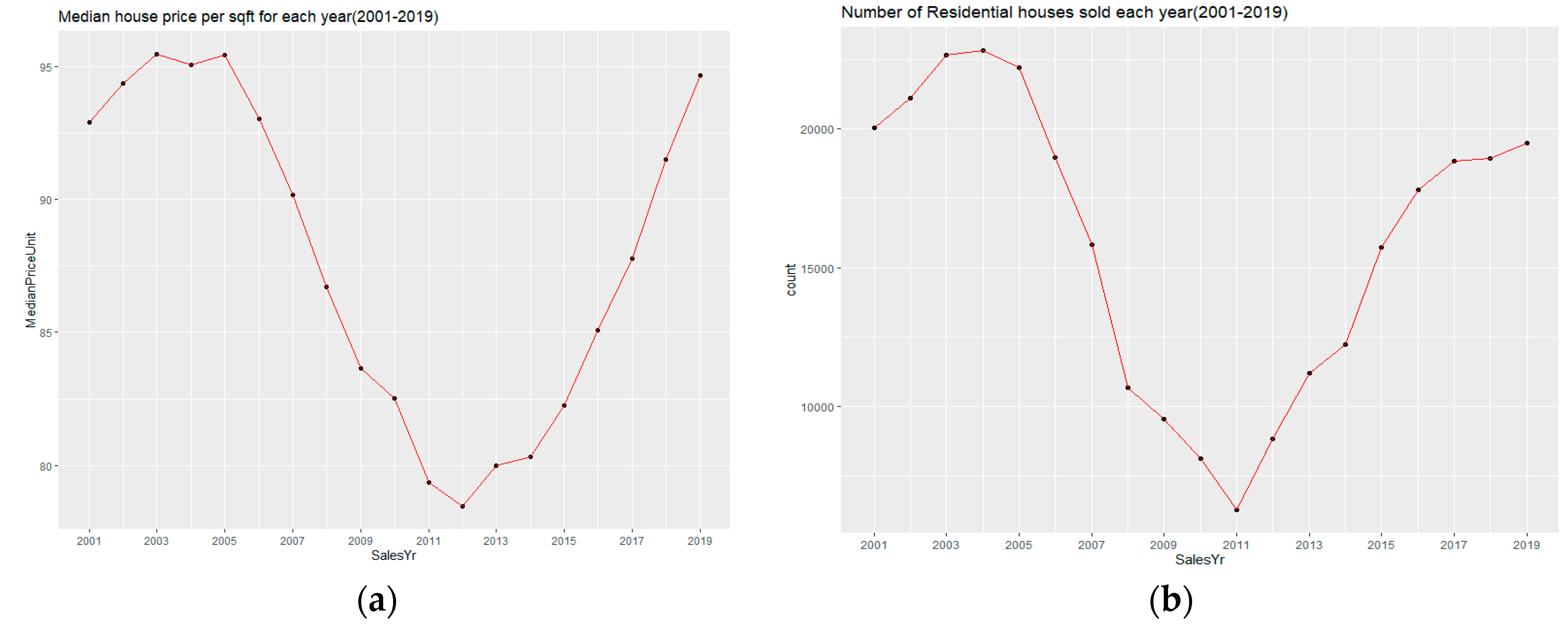
Figure 2 displays two annual time series trajectories: the 2001–2019 inflation-adjusted house prices per unit area (Figure 2a) and the number of residential house transactions (Figure 2b). Both graphs depict a generic V shape, demonstrating that the price values and transaction counts reached a peak during 2003–2005, dropped precipitously during and after the Great Recession (2007–2009), and then slowly bounced back during 2011–2019, which closely aligns with overall US housing market behavior statistics. As the price change due to the global factor occurred in the entire county, each submarket has the same change pattern and, hence, the RE estimation for each submarket based on the same trajectory is not expected to have a large variation.
Housing submarket boundaries delineated here utilized area aggregated spatial units (e.g., neighborhoods, school districts, zip code postal zone, census tracts, or census block groups), instead of individual housing units, for three main reasons. The first is the urban housing development process. House construction in urban areas is usually not by individuals, but rather by developers or builders in batch (which helps exploit economies of scale and minimize intermediate transport costs affiliated with agglomeration economies). It involves constructing hundreds of houses in tandem on an empty track of land, with economies of scale achieved through the utilization of similar house styles, building sizes, lot sizes, and other residential attributes, and the sharing of public infrastructure and services as well as local amenities. The second reason is that housing submarket boundaries derived from individual housing units are highly spatially fragmented. Hence, resulting submarkets barely have any practical meaning in real estate market analysis or urban policy planning. The third, and final, reason is that aggregating a large set of space–time house data into areal units and temporal intervals can compress data and significantly improve computational efficiency, which makes the submarket delineation of a large housing dataset with more than 300,000 records feasible. According to the US Census Bureau4, railroads, roads, streets, streams, bodies of water, or other visible physical boundaries or cultural features form census block group boundaries. A census block group usually contains 600–3000 people, a smaller areal unit than a census tract, school district, or zip code area, and is relatively homogeneous and compact. Thus, it is a midpoint between a fine (e.g., a parcel occupied by an individual housing unit) and a coarse spatial resolution (e.g., zip code postal zones and census tracts that frequently encompass too much heterogeneity), and, hence, can serve as an alternative to housing neighborhood boundaries. There are 887 census block groups in Franklin County and, therefore, the individual house data are reorganized into an 887-by-76 space–time data structure as follows: in the spatial dimension, 301,204 individual house data are aggregated into and summarized for 887 census block groups; and, in the temporal dimension, data are sliced first by year and then by quarter, resulting in 76 (=19 × 4) time intervals.

4.1. Salient Housing Attribute Variables

Clustering algorithms rely heavily on calculating feature separation (mostly Euclidian distance) among observations to determine similarity. Hence, the curse of dimensionality is a common issue when dealing with a high dimension of input attributes. To ensure that any latent spatial information is adequately considered, and resulting submarkets are interpretable and meaningful, a parsimonious set of variables with three non-spatial facets and two spatial traits is chosen as input into the algorithms. Notable is that prediction or forecasting hedonic price models that others have devised—two purposes that are beyond the scope of this paper—are likely to include not just three, but many, variables (e.g., Li and Li 2018). The three non-spatial variables—individual unit house price, house living area, and house age—are the most crucial determinants appearing in the literature for delineating submarkets. The two spatial attributes are the (x, y) coordinates of the census block group centroids. All variables were standardized to z-scores using the z-transformation.
Table 1 tabulates summary statistics for the five raw (i.e., pre-z-score) input variables. Whereas house price, living area, and house age are at the individual house level, the block group centroid (x, y) coordinates are at the aggregated areal unit level. The minimum value of house age is −2, denoting purchases for new houses not yet built at the time of sale. These raw variables are further processed and standardized as described next. The unit house price is the per house inflation-adjusted transaction price divided by its corresponding living area. The house age is number of years old at the time of sale. The individual house price per unit, living area, and house age are aggregated quarterly by each year within each block group boundary to estimate their median value, with these medians then concatenated into an 887-by-76 space–time data structure. With repeated temporal measurements in each analysis unit, the RE models can estimate stable temporal housing patterns with varying intercepts and no covariates. 
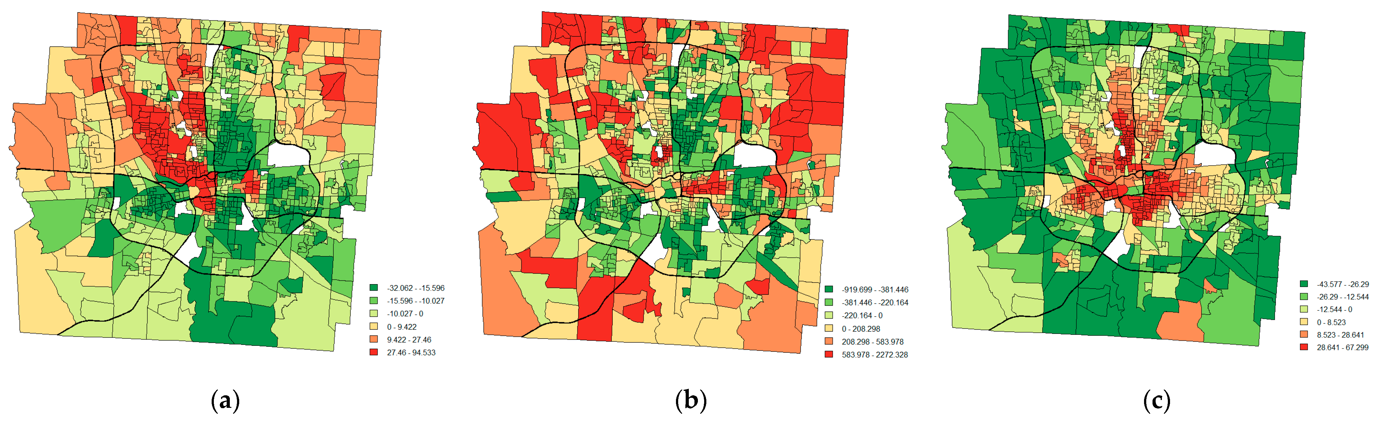
Figure 3 portrays plots of all the estimated RE terms in the study area, as well as prominent housing map patterns. Due to the presence of non-residential land-use zoning, 20 block groups with zero residential house transactions over 19 years were deleted from the study area, appearing as blank areas in the maps. Figure 3a portrays a high house value swath in the northern part, and conspicuous low value concentrations in the central and southern parts, of the county, with some exceptions in the inner city uptown. Figure 3b,c display an overall concentric zone pattern (i.e., the Burgess internal structure of the city spatial organization)—smaller, older buildings in the inner city, versus larger, newer edifices in the outer suburban areas.

4.2. An analytical Design for Delineating Housing Submarkets

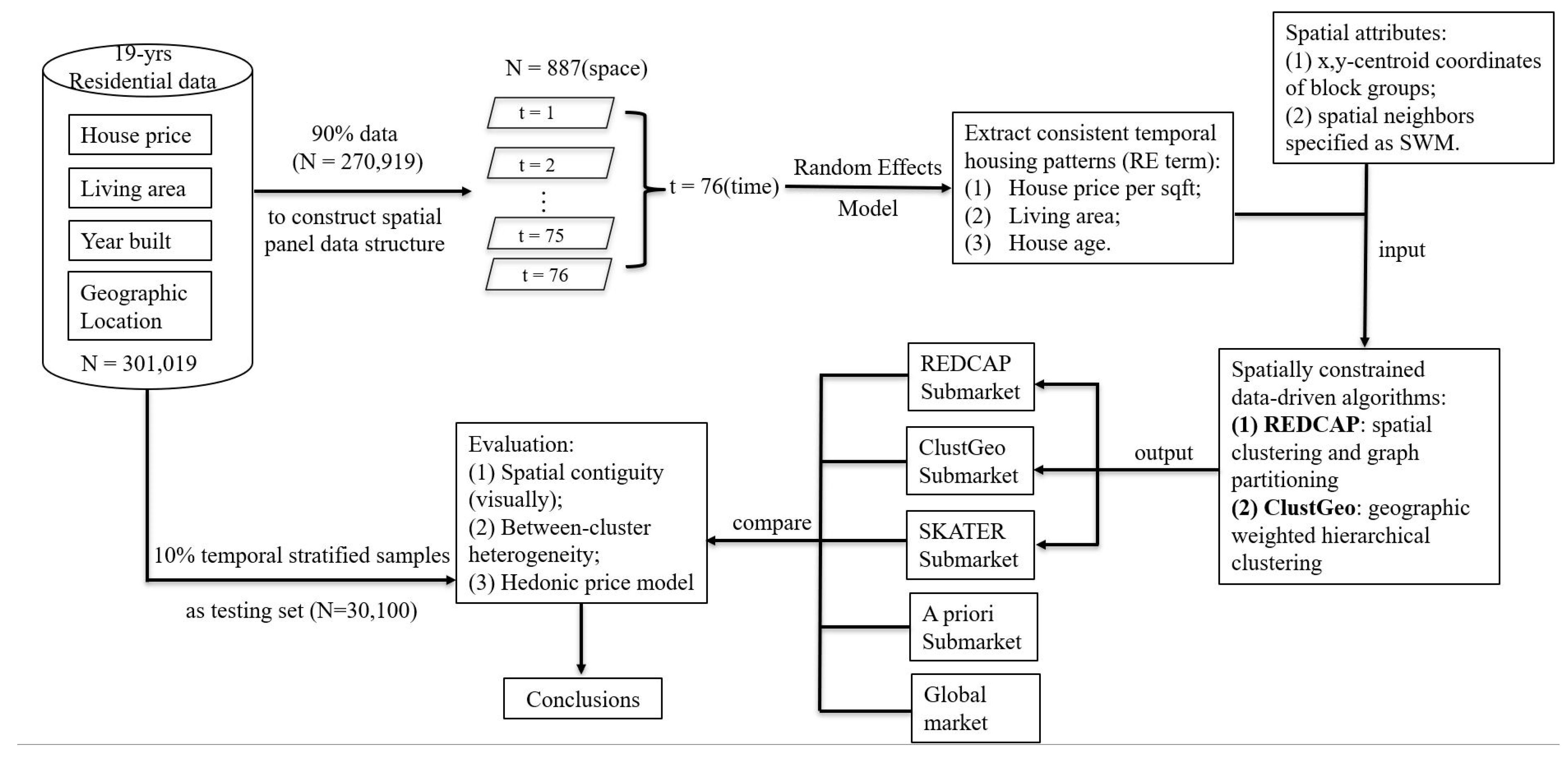
Figure 4 presents an analytical design comprising five steps. In step 1, the 19 years of Franklin County residential housing data are split into 2 datasets using a temporally stratified random sampling scheme. A sizeable amount, 90%, of the yearly stratified random sample draws is used as a training dataset to delineate the submarkets, with the remaining 10% of annual data used for testing and comparing the resulting submarkets. In step 2, the training data are aggregated and summarized at the census block group level to construct an 887-by-76 spatial panel dataset. In step 3, the RE term is estimated conditional on the attribute variables of house price per square footage, living area, and house age as the covariates, capturing consistent temporal housing patterns. In step 4, the RE terms are introduced in conjunction with spatial information into spatially constrained data-driven algorithms to delineate the Franklin County space–time housing submarkets. In the final stage, several alternative submarkets are examined and compared based upon the following three criteria: spatial contiguity, between-cluster heterogeneity, and model performance diagnostics. A 10% temporal stratified house sample with a composite size of 30,100 supplies an independent test dataset for evaluating model fit and price prediction errors of 5 hedonic price models, with and without submarkets.

5. Results

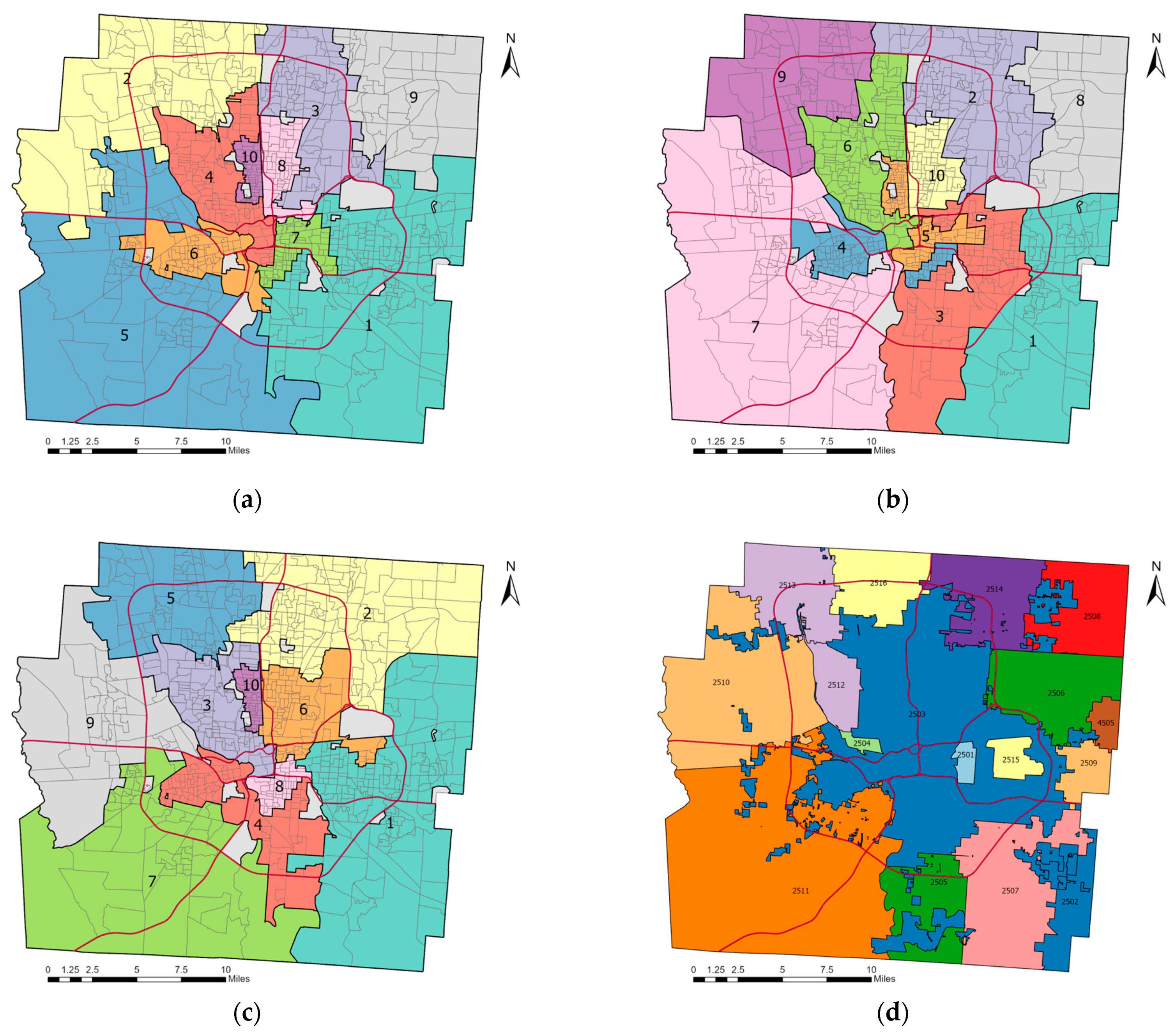
In order for the spatially constrained algorithms to be comparable, the number of clusters is set to 10 (i.e., the same constant). Each submarket is portrayed in a different color. Figure 5a reveals the REDCAP submarkets using Full-order constrained Ward linkage clustering (Full-Order-WLK) and Figure 5b is the ClustGeo submarkets map with K = 10 and α = 0.5 . Overall, two spatially constrained data-driven clustering algorithms generated similar results. Visually, the REDCAP and ClustGeo submarkets have similar regionalization patterns, both satisfying spatial closeness and compact clustering objectives. A minor difference between the two is that the REDCAP algorithm enforces a hard spatial contiguity constraint for each submarket, whereas the ClustGeo algorithm imposes a soft contiguity constraint for formulating submarkets. A hard spatial constraint means that two similar observations must share spatial boundaries to be grouped into one submarket. In contrast, a soft spatial constraint indicates that two observations with high non-spatial attribute similarity can be grouped into one submarket even if they are not spatially contiguous, although they exhibit a certain minimal degree of geographic similarity. This is the reason why Submarkets 4 and 5 in ClustGeo have two discontinuous parts in space (see Figure 5b).
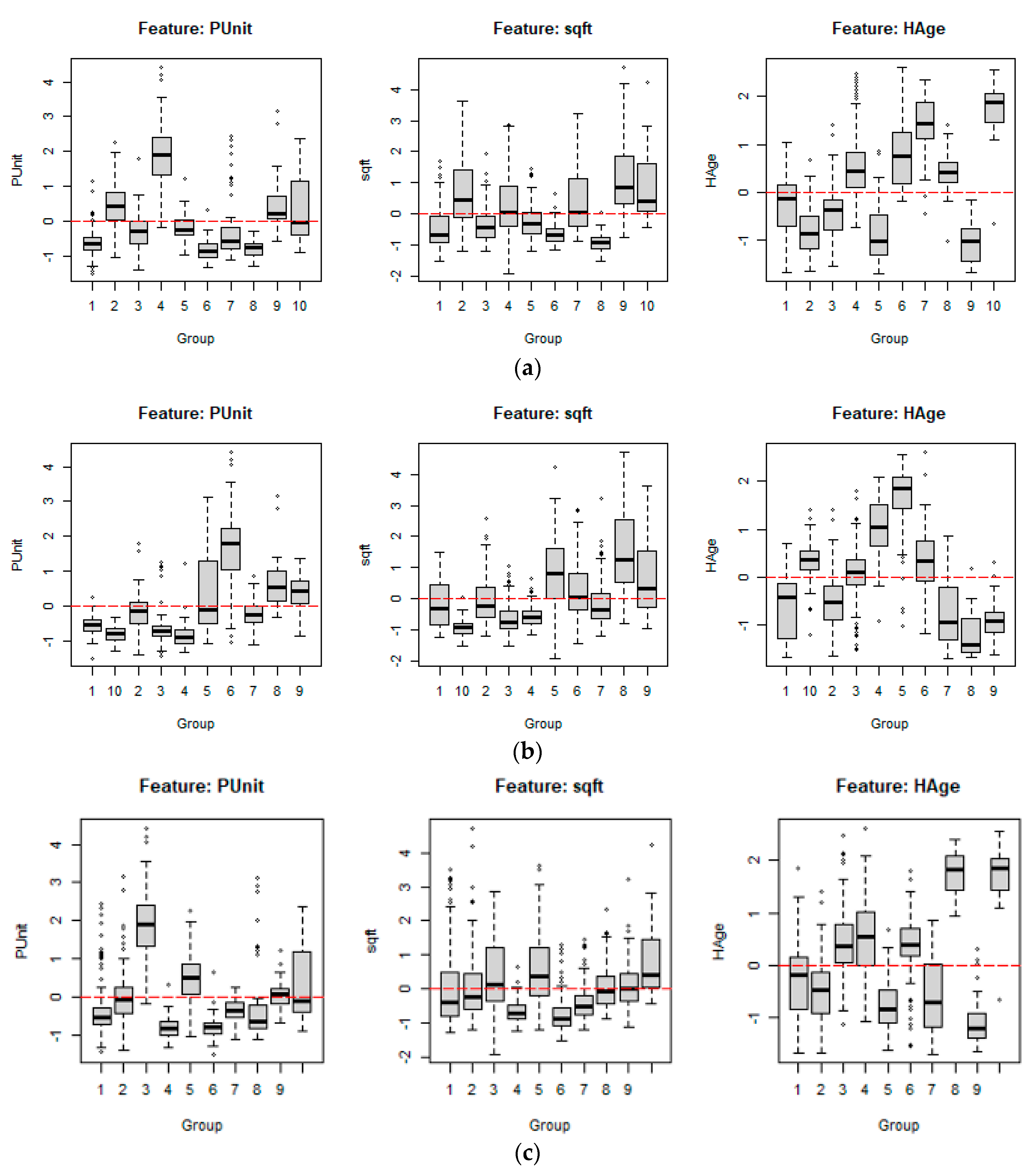
Figure 6a,b reproduce the boxplots of three non-spatial attribute similarity variables—house price per square footage, living area, and house age—together with the between-cluster heterogeneity for REDCAP as well as ClustGeo submarkets. These 2 sets of submarkets have similar between-cluster heterogeneity values: 0.656 and 0.644, respectively. The between-cluster heterogeneity index measures the ratio of the between- and total-cluster sums of squares and is widely adopted to evaluate uncovered clusters. Linking the boxplots with their corresponding submarket maps exposes that house age successfully differentiates between Franklin County inner and outer cities. Table 2 encapsulates the main attributes of each submarket. First, for REDCAP, low-priced, small houses in the outer city characterize Submarkets 1, 3, and 5; Submarkets 2 and 9 reflect mainly high-priced, middle-to-big sized houses in the outer city; Submarkets 6, 7, and 8 brand low-priced, small-to-mid-sized houses in the inner city; and mid-to-high-priced, big houses in the inner city stamp Submarkets 4 and 10. Second, for ClustGeo, Submarkets 1, 3, and 7 embrace primarily low-priced, small-to-mid-sized houses in the outer city; Submarkets 8 and 9 encompass high-priced, big houses in the outer city; Submarket 2 embodies mid-priced and mid-sized houses in the outer city; Submarkets 4 and 10 mostly consist of low-priced, small houses in the inner city; and Submarket 5 contains mid-priced and mid-sized houses in the inner city, Submarket 6 is labeled as high-priced, mid-sized houses in the inner city.
Figure 5c,d show the SKATER and a priori submarkets, the latter included as a reference map. Figure 6c pictures the SKATER submarket housing characteristic boxplots. Comparing the cluster heterogeneity value and boxplot statistics confirms that the REDCAP approach performs better than the alternative SKATER algorithm in identifying distinct clusters. Thus, the REDCAP with Full-Order-WLK is superior to the SKATER approach, at least in this case, just like the author of the REDCAP method claims. Figure 5d displays the 17 school district boundaries within Franklin County that serve as a priori submarkets6, included here because a common traditional a priori framework practice is to demarcate with school district boundaries or municipal administrative borders. These Franklin County school district boundaries are not necessarily spatially contiguous, as is illustrated by the Columbus ISD (encoded 2503 in the map). The lack of coterminousness stems from the spatially fragmented administrative boundaries of the City of Columbus.
The 10% testing data subset was utilized to examine the performance of the 5 hedonic price models coupled with each of the 4 sets of submarkets: submarket absence (model 1), 17 a priori submarkets (model 2), SKATER submarkets (model 3), REDCAP submarkets (model 4), and ClustGeo submarkets (model 5). All submarkets are encoded with binary 0–1 dummy variables in their respective specifications. Model performance criteria consist of both the Akaike (AIC) and Bayesian information criterion (BIC), in addition to a pseudo-R-squared value (R2) and root mean squared error (RMSE), two of the most popular goodness-of-fit measures for model comparisons (e.g., Wheeler et al. 2014; Hu et al. 2022). Table 3 reveals that the hedonic price model with REDCAP submarkets (model 4) has the best combination of overall model fit and lowest prediction error. The pseudo-R2 value increases from 0.7382 for model 1, to 0.7734, 0.8042, and 0.8210, respectively, for models 2, 3, and 4, decreasing slightly to 0.8112 for model 5. The AIC and BIC display the same trend across these five model specifications. Furthermore, models 4 and 5, with respective REDCAP and ClustGeo submarkets, have the lowest prediction errors, as rated by their RMSE values. Levene’s test results in Table 4 show that each set of submarkets exhibits statistically significant between-segments house price variance, with REDCAP yielding the largest F value that indicates a difference across submarkets. In other words, each submarket set contains markedly excess house price variability.
This empirical case study using a 19-year Franklin County, OH, house price dataset renders the following implications. First, all hedonic regression models with submarkets have a better model fit and lower prediction errors than a posited model with no submarket. This argues for the presence of house submarkets in Franklin County, a contention that agrees with the existing housing submarket literature. Second, in terms of three particular evaluation criteria, the spatially constrained data-driven demarcated submarkets (SKATER, REDCAP, and ClustGeo) outperform the a priori submarkets. All else being equal, the usual expectation is that a statistical model whose specification includes more subgroups will improve its model fit and reduce its prediction error. However, here, hedonic price models 3, 4, and 5 with only 10 submarkets perform better than a prevailing wisdom-based a priori submarket with 17 subgroups based upon public school districts. Third, not surprisingly, the REDCAP submarket is superior to the SKATER submarket, because SKATER is a naïve case of REDCAP. Fourth, in this empirical study, the model with REDCAP-delineated submarkets appears to excel in all five hedonic price models, capturing the highest cluster heterogeneity. However, the difference between REDCAP and ClustGeo may not be statistically significant because their statistic values are relatively close, and a visual inspection of their resulting submarket structures suggests that they appear to be similar. Therefore, overall, the proposed REDCAP and ClustGeo approaches perform equally well. Both algorithms successfully segmented the study area into inner-city and outer-city submarkets, spawning similar regionalization structures, despite some differences in their submarket boundaries. Finally, neither of the spatially constrained data-driven algorithms adopted in this study needs to specify the number of submarkets (K) beforehand, unlike K-means or DBSCAN. The arbitrariness of a choice of this K is one of the main criticisms leveled at certain popular clustering algorithms, such as K-means, the EM algorithm for a Gaussian mixture model, or DBSCAN. Due to their inherent mechanisms, different options of K can result in a given algorithm creating very different cluster structures. In contrast, both the ClustGeo and REDCAP algorithms are based upon agglomerative hierarchical clustering, meaning that clusters are hierarchically nested with varying K. In addition, these latter algorithms generate scree plots and dendrograms to uncover the finer structure within and between clusters to help choose an optimal K number of submarkets for a specific dataset.

6. Discussion and Conclusions

The study précised in this paper aimed to delineate stable and reliable space–time housing submarkets with a large spatiotemporal house sales dataset. Quantification of its temporal dimension was by extracting consistent and statistically significant patterns with RE model specifications. The spatial dimension disclosure was through implementing two spatially constrained data-driven segmentation approaches. The empirical case study using a 19-year Franklin County, OH, space–time house price dataset illustrates that these approaches perform better than non-spatial methods and a priori preset spatial boundaries.
Spatial constraints were imposed in this submarket segmentation study at three different levels. First, individual houses were aggregated into census block groups as the base unit for formulating submarkets, thus reducing computational burdens and spatial fragmentation. Second, the absolute location, the individual (x, y) coordinates of block group centroids, was included as a pair of input covariates to incorporate a reasonable proxy for spatial proximity. Third, spatial propinquity (spatial neighbors) or topology was specified in the data-driven clustering or partitioning algorithms to ensure enforcement of soft or hard spatial contiguity.
This paper contributes to the existing literature in various ways. First, it helps fill the literature gap about space–time house submarket delineation, primarily focusing on the stability of space–time submarkets. It proposes an analytical framework of combining the RE model with a spatially constrained data-driven approach to demarcate space-specific and time-invariant housing submarkets. A large quantity of spatial panel house transaction data in this study allowed for a rather comprehensive examination of this method. Second, the resulting demarcations produced practical and meaningful submarket boundaries by taking spatial closeness, spatial contiguity, and area-aggregated spatial census geography units into account. Third, the results summarized here demonstrate the superiority of the REDCAP and ClustGeo algorithms for spatial housing submarket delineation. Such applications of these two spatially constrained data-driven algorithms in housing submarket delineation are relatively novel. Although several papers already describe the use of SKATER, the naïve version of REDCAP, by itself for housing submarket delineation (e.g., Helbich et al. 2013), this paper presents a comparative analysis of three spatially constrained data-driven algorithms—SKATER, REDCAP, and ClustGeo. This comparison yields a practical implication that the data-driven approach can enhance spatial housing submarket demarcation. Third, this paper explores different ways of incorporating space into data-driven unsupervised (hierarchical clustering) machine learning algorithms. Accordingly, it should serve to inspire geospatial researchers to reflect on what roles space can play in machine learning methods, and encourage more data scientists to incorporate geographic locations, spatial autocorrelation, and/or spatial topology into current artificial intelligence (AI) algorithms to bring forth new spatially explicit models and bolster the cutting-edge research area of GeoAI. Finally, this paper furnishes an enhanced tool to generate housing submarkets, which is recognized as a crucial component for strategic housing investment and housing market operations (Jones 2002; Jones et al. 2004). This achievement can be useful for, especially, local or regional policy practitioners who are responsible for solving housing problems in relatively small areas such as a metropolitan area. Although the modeling framework articulated here can be applied to other areas, it may need selected customizing to adapt it to geographic landscape specific local characteristics.
Based upon findings summarized in this paper, some topics are worth exploring in future work. First, similar studies can also be undertaken for other coarser geographic resolution levels, such as zip code areas or census tracts. In theory, house homogeneity is harder to guarantee within coarser spatial units, but comparing the resulting submarkets derived from different aggregate areal units spanning a range of coarseness seems like a worthwhile endeavor. Second, even though this paper targets macro-level stable space–time submarkets, the investigation of housing submarket dynamics at the micro-level would be a valuable future exercise. For example, impacts of inner-city gentrification, or of a newly built highway, on house prices or submarkets. Third, the proposed method is tested only with RE. Although this component is a popular ingredient in space–time modeling, other approaches, including fixed and multi-level effects, can also provide compatible outcomes. Further investigations with a myriad of other approaches can help establish a more comprehensive understanding of housing submarket delineation.

Author Contributions

Conceptualization and design, M.C., Y.C. and D.A.G.; writing—original draft preparation, M.C.; writing—review and editing, Y.C. and D.A.G.; supervision, Y.C. and D.A.G. All authors have read and agreed to the published version of the manuscript.

Funding

This research received no external funding.

Data Availability Statement

The data presented in this study are available upon request from the corresponding author; it also is downloadable from a cited public portal.

Acknowledgments

The first author thanks Michael Tiefelsdorf for his comments.

Conflicts of Interest

The authors declare no conflict of interest.

Appendix A

The house sale data for the empirical data analysis including the characteristics and the locations of houses were downloaded from the Franklin County Auditor website (https://audr-apps.franklincountyohio.gov/reporter accessed on 27 May 2023).

Notes

1
The average annual growth rate is reported by USA Facts that reports population and demographic changes in the USA using census data. Available online: https://usafacts.org/data/topics/people-society/population-and-demographics/our-changing-population/. Its last access was on 27 May 2023.
2
Data cleaning mainly consists of deleting irregular sales, such as those with only land, multiple-parcels, non-residential buildings (e.g., those with 0 bedrooms), apartment complexes, when total building area is less than 200 square feet, or when a house price (inflation-adjusted) is below $41,921 (the 10th percentile of transaction prices).
3
4
Geographic Areas Reference Manual. Available online: https://www2.census.gov/geo/pdfs/reference/GARM/Ch11GARM.pdf, accessed on 27 May 2023.
5
The data were obtained from the Franklin County Auditor open data portal. Technically, Franklin County has 21 school districts, of which 4 are at the fringe of the county boundary, resulting in them appearing as tiny polygon fragments. Thus, for this paper, these small partial territories were merged into surrounding primary school districts.
6
A judicious merging of selected adjacent peripheral school districts located along the county boundary line reduces them to 10 submarkets, for a more meaningful comparison.

References

  1. An, Li, Ming Hsiang Tsou, Stephen E. S. Crook, Yongwan Chun, Brian Spitzberg, J. Mark Gawron, and Dipak K. Gupta. 2015. Space–Time Analysis: Concepts, Quantitative Methods, and Future Directions. Annals of the Association of American Geographers 105: 891–914. [Google Scholar] [CrossRef]
  2. Assunção, Renato M., Marcos Corrêa Neves, Gilberto Câmara, and Corina da Costa Freitas. 2006. Efficient Regionalization Techniques for Socio-Economic Geographical Units Using Minimum Spanning Trees. International Journal of Geographical Information Science 20: 797–811. [Google Scholar] [CrossRef]
  3. Bourassa, Steven C., Eva Cantoni, and Martin Hoesli. 2010. Predicting House Prices with Spatial Dependence: A Comparison of Alternative Methods. Journal of Real Estate Research 32: 139–59. [Google Scholar] [CrossRef]
  4. Bourassa, Steven C., Foort Hamelink, Martin Hoesli, and Bryan D. Macgregor. 1999. Defining Housing Submarkets. Journal of Housing Economics 8: 160–83. [Google Scholar] [CrossRef]
  5. Bourassa, Steven C., Martin Hoesli, and Vincent S. Peng. 2003. Do Housing Submarkets Really Matter? Journal of Housing Economics 12: 12–28. [Google Scholar] [CrossRef] [Green Version]
  6. Can, Ayse. 1992. Specification and Estimation of Hedonic Housing Price Models. Regional Science and Urban Economics 22: 453–74. [Google Scholar] [CrossRef]
  7. Chavent, Marie, Vanessa Kuentz-Simonet, Amaury Labenne, and Jérôme Saracco. 2018. ClustGeo: An R Package for Hierarchical Clustering with Spatial Constraints. Computational Statistics 33: 1799–822. [Google Scholar] [CrossRef] [Green Version]
  8. Chen, Zhuo, Seong-Hoon Cho, Neelam Poudyal, and Roland K. Roberts. 2009. Forecasting housing prices under different market segmentation assumptions. Urban Studies 46: 167–87. [Google Scholar] [CrossRef]
  9. Chun, Yongwan. 2014. Analyzing Space-Time Crime Incidents Using Eigenvector Spatial Filtering: An Application to Vehicle Burglary. Geographical Analysis 46: 165–84. [Google Scholar] [CrossRef]
  10. Cohen, Jeffrey P., Yannis M. Ioannides, and Win Thanapisitikul. 2016. Spatial Effects and House Price Dynamics in the USA. Journal of Housing Economics 31: 1–13. [Google Scholar] [CrossRef]
  11. Geng, Bin, Haijun Bao, and Ying Liang. 2015. A Study of the Effect of a High-Speed Rail Station on Spatial Variations in Housing Price Based on the Hedonic Model. Habitat International 49: 333–39. [Google Scholar] [CrossRef]
  12. Goodman, Allen C., and Thomas G. Thibodeau. 1998. Housing Market Segmentation. Journal of Housing Economics 7: 121–43. [Google Scholar] [CrossRef]
  13. Goodman, Allen C., and Thomas G. Thibodeau. 2003. Housing Market Segmentation and Hedonic Prediction Accuracy. Journal of Housing Economics 12: 181–201. [Google Scholar] [CrossRef] [Green Version]
  14. Goodman, Allen C., and Thomas G. Thibodeau. 2007. The spatial proximity of metropolitan area housing submarkets. Real Estate Economics 35: 209–32. [Google Scholar] [CrossRef]
  15. Griffith, Daniel A., Yongwan Chun, and Bin Li. 2019. Spatial Regression Analysis Using Eigenvector Spatial Filtering. London: Academic Press. [Google Scholar]
  16. Guo, D. 2008. Regionalization with Dynamically Constrained Agglomerative Clustering and Partitioning (REDCAP). International Journal of Geographical Information Science 22: 801–23. [Google Scholar] [CrossRef]
  17. Helbich, Marco, Wolfgang Brunauer, Julian Hagenauer, and Michael Leitner. 2013. Data-Driven Regionalization of Housing Markets. Annals of the Association of American Geographers 103: 871–89. [Google Scholar] [CrossRef]
  18. Hu, Lan, Daniel A. Griffith, and Yongwan Chun. 2018. Space-Time Statistical Insights about Geographic Variation in Lung Cancer Incidence Rates: Florida, USA, 2000–2011. International Journal of Environmental Research and Public Health 15: 2406. [Google Scholar] [CrossRef] [Green Version]
  19. Hu, Jin, Xuelei Xiong, Yuanyuan Cai, and Feng Yuan. 2020. The Ripple Effect and Spatiotemporal Dynamics of Intra-Urban Housing Prices at the Submarket Level In Shanghai, China. Sustainability 12: 5073. [Google Scholar] [CrossRef]
  20. Hu, Lan, Yongwan Chun, and Daniel A. Griffith. 2022. Incorporating spatial autocorrelation into house sale price prediction using random forest model. Transactions in GIS 26: 2123–44. [Google Scholar] [CrossRef]
  21. Hwang, Sungsoon, and Jean-Claude Thill. 2009. Delineating Urban Housing Submarkets with Fuzzy Clustering. Environment and Planning B: Planning and Design 36: 865–82. [Google Scholar] [CrossRef]
  22. Jones, Colin. 2002. The definition of housing market areas and strategic planning. Urban Studies 39: 549–64. [Google Scholar] [CrossRef]
  23. Jones, Colin, Chris Leishman, and Craig Watkins. 2004. Intra-urban migration and housing submarkets: Theory and evidence. Housing Studies 19: 269–83. [Google Scholar] [CrossRef]
  24. Jones, Colin, Chris Leishman, and Craig Watkins. 2005. Housing market processes, urban housing submarkets and planning policy. The Town Planning Review 76: 215–33. [Google Scholar] [CrossRef]
  25. Kauko, Tom. 2004. A Comparative Perspective on Urban Spatial Housing Market Structure: Some More Evidence of Local Sub-Markets Based on a Neural Network Classification of Amsterdam. Urban Studies 41: 2555–79. [Google Scholar] [CrossRef]
  26. Keskin, Berna, and Craig Watkins. 2017. Defining Spatial Housing Submarkets: Exploring the Case for Expert Delineated Boundaries. Urban Studies 54: 1446–62. [Google Scholar] [CrossRef] [Green Version]
  27. Kopczewska, Katarzyna, and Piotr Ćwiakowski. 2021. Spatio-Temporal Stability of Housing Submarkets. Tracking Spatial Location of Clusters of Geographically Weighted Regression Estimates of Price Determinants. Land Use Policy 103: 105292. [Google Scholar] [CrossRef]
  28. Li, Rita Yi Man, and Herro Ching Yu Li. 2018. Have housing prices gone with the smelly wind? Big data analysis on landfill in Hong Kong. Sustainability 10: 341. [Google Scholar] [CrossRef] [Green Version]
  29. Mulligan, Gordon F., Adrian X. Esparza, and Rachel Franklin. 2002. Housing Prices in Tucson, Arizona. Urban Geography 23: 446–70. [Google Scholar] [CrossRef]
  30. Ottensmann, John R., Seth Payton, and Joyce Man. 2008. Urban Location and Housing Prices within a Hedonic Model. Journal of Regional Analysis and Policy 38: 19–35. [Google Scholar] [CrossRef]
  31. Pryce, Gwilym. 2013. Housing submarkets and the lattice of substitution. Urban Studies 50: 2682–99. [Google Scholar] [CrossRef]
  32. Shimizu, Chihiro, Hideoki Takatsuji, Hiroya Ono, and Kiyohiko G. Nishimura. 2010. Structural and Temporal Changes in the Housing Market and Hedonic Housing Price Indices. International Journal of Housing Markets and Analysis 3: 351–68. [Google Scholar] [CrossRef] [Green Version]
  33. Sirmans, Stacy, David Macpherson, and Emily Zietz. 2005. The composition of hedonic pricing models. Journal of Real Estate Literature 13: 1–44. [Google Scholar] [CrossRef]
  34. Soltani, Ali, Christopher James, Pettit Mohammad, and Heydari Fatemeh. 2021. Housing Price Variations Using Spatio-Temporal Data Mining Techniques. Journal of Housing and the Built Environment 36: 1199–227. [Google Scholar] [CrossRef]
  35. Straszheim, Mahlon R. 1975. An Econometric Analysis of the Urban Housing Market. New York: Bureau of Economic Research. [Google Scholar]
  36. Usman, Hamza, Mohd Lizam, and Muhammad Usman Adekunle. 2020. Property Price Modelling, Market Segmentation and Submarket Classifications: A Review. Real Estate Management and Valuation 28: 24–35. [Google Scholar] [CrossRef]
  37. Watkins, Craig A. 2001. The Definition and Identification of Housing Submarkets. Environment and Planning A 33: 2235–53. [Google Scholar] [CrossRef]
  38. Wheeler, David. C., Antonio Páez, Jamie Spinney, and Lance A. Waller. 2014. A Bayesian approach to hedonic price analysis. Papers in Regional Science 93: 663–83. [Google Scholar] [CrossRef]
  39. Wu, Changshan, and Rashi Sharma. 2012. Housing Submarket Classification: The Role of Spatial Contiguity. Applied Geography 32: 746–56. [Google Scholar] [CrossRef]
  40. Wu, Chao, Fu Ren, Wei Hu, and Qingyun Du. 2019. Multiscale Geographically and Temporally Weighted Regression: Exploring the Spatiotemporal Determinants of Housing Prices. International Journal of Geographical Information Science 33: 489–511. [Google Scholar] [CrossRef]
  41. Wu, Chao, Xinyue Ye, Fu Ren, and Qingyun Du. 2018. Modified Data-Driven Framework for Housing Market Segmentation. Journal of Urban Planning and Development 144: 04018036. [Google Scholar] [CrossRef]
  42. Xiao, Yang. 2017. Urban Morphology and Housing Market. Singapore: Springer. [Google Scholar]
  43. Yuan, Feng, Jiawei Wu, Yehua Dennis Wei, and Lei Wang. 2018. Policy Change, Amenity, and Spatiotemporal Dynamics of Housing Prices in Nanjing, China. Land Use Policy 75: 225–36. [Google Scholar] [CrossRef]
Figure 1. Spatial variation of house prices in Franklin County, OH.
Jrfm 16 00291 g001
Figure 2. Temporal trajectory of residential house transaction data in Franklin County, OH, 2001–2019. (a) Median house price per square footage by year; (b) Count of transactions by year.
Jrfm 16 00291 g002
Figure 3. Quantile choropleth maps depicting three estimated RE terms representing the time-invariant and space-specific housing patterns (exhibiting conspicuous positive spatial autocorrelation) over 19 years. (a) house price per square footage; (b) house living area; (c) house age.
Jrfm 16 00291 g003
Figure 4. An analytic design for delineating space–time housing submarkets.
Jrfm 16 00291 g004
Figure 5. Ten submarkets constructed with four methods. (a) REDCAP output; (b) ClustGeo output; (c) SKATER outputs; (d) A priori submarkets delineated by 17 School district boundaries5. Note that the numbers are arbitrary submarket IDs for each outcome.
Jrfm 16 00291 g005
Figure 6. Boxplots of submarket house characteristics by three geographic clustering methods. (a) REDCAP; (b) ClustGeo; (c) SKATER.
Jrfm 16 00291 g006
Table 1. Raw data variable summary statistics.
VariablesnMinQ1MedianMeanQ3Max
House price301,01941,922100,946136,479162,603188,9333,155,512
Living area301,019280115215051681203315,090
House age301,019−2102532.2549218
X coordinate8871,763,7651,811,4671,831,7171,831,0971,848,8381,889,445
Y coordinate887662,696709,640726,629728,506748,727778,628
Note: Data were obtained from the Franklin County Auditor.
Table 2. Characteristics of REDCAP and ClustGeo submarkets.
VariablesSubmarkets CharacteristicsREDCAP Submarket LabelsClustGeo Submarket Labels
House ageInner city (older houses)4, 6, 7, 8, 104, 5, 6, 10
Outer city (newer houses)1, 2, 3, 5, 91, 2, 3, 7, 8, 9
Unit house priceHigh-priced houses2, 4, 96, 8, 9
Mid-priced houses102, 5
Low-priced houses1, 3, 5, 6, 7, 81, 3, 4, 7, 10
Total living areaBig houses25, 8, 9
Mid-sized houses4, 7, 9, 101, 2, 6
Table 3. Selected hedonic regression model performance comparisons of submarket absence, a priori submarkets, and spatially constrained submarkets.
Hedonic Price ModelsPseudo R2AICBICRMSE
Base modelModel 1: submarket absence0.73824138.714529.3858,260.5
A priori submarkets
(K = 17)
Model 2: school district submarkets 0.7734−170.62353.0452,690.84
Spatially constrained submarkets (K = 10)Model 3: SKATER0.8042−4575.90−4110.4254,004.93
Model 4: REDCAP 0.8210−7276.80−6811.3251,412.45
Model 5: ClustGeo 0.8112−5677.24−5211.7651,795.31
Table 4. Levene’s test results for submarket variance equality.
MethodDfF Valuep-Value
A priori submarkets (K = 17)School district 1680.4240.0000
Spatially constrained
submarkets (K = 10)
SKATER9100.800.0000
REDCAP 9183.210.0000
ClustGeo 9130.140.0000
Disclaimer/Publisher’s Note: The statements, opinions and data contained in all publications are solely those of the individual author(s) and contributor(s) and not of MDPI and/or the editor(s). MDPI and/or the editor(s) disclaim responsibility for any injury to people or property resulting from any ideas, methods, instructions or products referred to in the content.

