A Rank Estimator Approach to Modeling Default Frequencies

Abstract

This study introduces a non-parametric methodology for estimating expected frequencies of defaults and other credit events. The methodology allows for an independent estimation of a credit-quality variable, referred to as a default rank variable. In a subsequent step, the relationship between the rank variable and the expected default frequency is established. This analysis can be achieved by initially determining the functional dependence between the rank variable and the expected tail default frequencies representing the average default frequencies of entities ranked lower than a given rank value. The expected default frequency can then be derived from a simple linear integral equation. We propose a prototype model for public corporations which establishes generalized logistic function dependencies between the distance-to-default rank variable and the expected default frequencies in the log–log space. This relationship applies to public corporations across different credit rating categories.

1. Introduction

Analysis of the credit risk of bond portfolios requires estimation of the frequency and severity of potential credit events involving the bond issuer entities. Severity estimation involves assessing the extent of losses incurred in a credit event. Expected frequencies represent probability estimates of these credit events occurring. To estimate the expected default frequencies (EDFs), analysts often turn to average historical default rates within agency credit rating categories, which are often adjusted for credit cycles. For instance, Gupton et al. (1997) utilized this method to determine the default component in a portfolio’s loss distribution. One notable advantage of this approach is the widespread availability of agency ratings for various types of issuers, including public and private corporations, sovereign entities, and municipalities. Rating agencies possess extensive experience in assessing the creditworthiness of diverse issuers and have access to non-public information; however, a drawback of the rating-based approach is its failure to account for variations in the credit quality among entities with the same rating. In essence, while credit ratings provide the average EDF, they do not elucidate the variability within the EDFs of the rating categories. Over the years, various methods that are independent of agency ratings for estimating EDFs have emerged. In the realm of corporate issuers, Chava and Jarrow (2004) employed a hazard rate to estimate expected bankruptcy frequencies, while Campbell et al. (2008) utilized a logistic model. The KMV model, discussed by Kealhofer (2003a), uses a distance-to-default (DD) metric as an explanatory variable for modeling public corporate EDFs. A notable advantage of this approach is that DD is a simple metric that has impressive power to rank firms according to their default risk (see, e.g., Bharath and Shumway (2008)). For sovereign entities, an approach utilizing a metric similar to DD was developed by Gray et al. (2007) and in Gapen et al. (2008). Another significant source of credit risk originates from the credit rating transitions of bond issuer entities. Similar to the analysis of default risk, historical average transition rates between agency credit rating categories are commonly employed in this analysis. In addition, similar to the case of default risk, this approach does not account for the variations among entities within these categories. To address this issue, econometric models are often introduced, incorporating a credit-quality variable for issuers with a fixed rating. These models derive transition probabilities that depend on the initial value and dynamics of this variable. This approach is discussed in detail by Frey and McNeil (2003). A model that utilizes DD as the credit-quality variable was presented by Gordy and Heitfield (2001).

The statistical techniques used to model EDFs can be categorized as parametric and nonparametric models. Parametric models, such as the hazard rate and logistic models, provide precise functional inferences about how EDFs depend on covariates. While specifying the EDF as a logistic function of covariates is conceptually simple, the choice of the logistic function may not optimally reflect the data. Other parametric models face similar issues. The philosophy behind the KMV model differs from this. The DD metric is specialized to become an optimal variable for ranking corporations based on their credit quality. A subsequent problem to address is finding the EDF function, which represents the relationship between the entity specific DD variable and the associated EDF. The precise form of KMV’s DD or the EDF function is not publicly known. While there is a significant amount of literature available on finding a DD metric that aligns well with the KMV model, there has been minimal focus on making inferences about the shape of the EDF function. Interested readers can find discussions about the KMV’s DD in references by Duffie and Singleton (2003), Kealhofer (2003a), Bharath and Shumway (2008), and Jessen and Lando (2015).

This study introduces a novel econometric methodology for nonparametric inference about EDFs. The approach begins by identifying a credit-quality variable, referred to as the rank variable, which enables the ranking of entities from the most likely to experience a default event to least likely. The subsequent step involves an initial estimation of the expected tail default frequencies (ETDFs) for all rank values. These ETDFs represent the average default frequencies of entities ranked lower than a reference rank value r. The ETDFs are linked to the EDFs through a simple Volterra integral equation of the first kind. Under a mild differentiability condition regarding the specification of the ETDFs, the EDFs can be determined analytically from this relationship. The estimation is initially performed for the ETDFs instead of EDFs because the ETDF estimator allows larger samples and as such results in smaller estimation errors. This methodology can be applied to estimate the expected credit rating transition frequencies as well. This modeling approach separates the task of finding the rank variable from the process of finding the EDF estimates. This sets it apart from common frequency estimation techniques, such as the logistic models often used in frequency modeling.

In this paper, we study public corporations in more detail. We construct a prototype model that elucidates the relationship between the DD rank variable and EDFs within various credit rating categories for these corporations. These models specifically shed light on the variations in EDFs among corporations sharing the same credit rating. Public corporations are a natural domain of application, as the problem of ranking these entities according to their credit quality has been extensively studied. Empirical analysis supports the use of the DD metric as the rank variable, as suggested by Kealhofer (2003a), Bharath and Shumway (2008), and Jessen and Lando (2015). The challenge in establishing the relationship between the DD and EDFs primarily lies in the substantial data requirements. Notably, defaults among investment-grade-rated corporations are very infrequent. Successfully modeling this dependence requires a historical dataset encompassing corporate defaults and additional market observables spanning several decades. Obtaining such comprehensive datasets can prove challenging. The prototype model we propose addresses this issue by incorporating specific assumptions about EDFs in order to employ a data reduction strategy. We critically analyze these assumptions and discuss a strategy to weaken their impact. With data reduction in place, the models yield a logistic function-based relationship between DDs and EDFs in the log–log space for each rating category. EDFs can fluctuate within rating-specific upper and lower bounds. The variability among log-EDFs for different corporations within these bounds is governed by the logistic function’s dependency on log-DDs. This prototype model may be considered as a statistical template for the credit event frequency modeling under this paradigm. This manuscript explains in detail how to estimate a model specified in this way.

The EDF finds essential applications in estimating risk metrics for portfolios exposed to credit risk and in valuing securities with values that are dependent on the likelihoods of future defaults. Under the minimal requirements outlined by Basel II, the portfolio’s expected loss is to be analyzed using an annual horizon. The EDF serves as a fundamental component in calculating the expected loss, as explained by Crouhy et al. (2000) and Stephanou and Mendoza (2005). Corporate bond valuation models that use EDFs to measure the credit contribution in the price (i.e., the credit spread) are discussed in Bohn (2000), Kealhofer (2003b), and Denzler et al. (2006). Credit default swap pricing using the EDF is explained in Hull and White (2000). In addition, Berndt et al. (2018) used the EDF to measure the credit risk premium in credit market securities. Within a credit rating category, the ranking of entities in terms of their credit quality offers valuable insights into the relative disparities in credit quality among different issuers, going beyond their credit ratings. This ranking helps in identifying entities that are likely to face credit rating downgrades or upgrades. Credit transitions in risk management have been discussed by McNeil et al. (2005).

The general modeling framework, which is the novel theory contribution of this manuscript, is introduced in Section 2. Subsequently, in Section 3 we construct prototype EDF models for public corporations across various credit ratings. The objective of Section 2 is to elucidate, under reasonable assumptions, the types of dependencies that are expected from the general framework. This exploration leads to a novel insight into the logistic log–DD and log–EDF relationships. Finally, the conclusion touches upon potential future directions for this methodology.

2. Rank Estimators for Expected Default Frequencies

In this section we consider time dependent populations of bond issuer entities. Each population is determined by its credit rating, and the members represent the entities that are assigned this rating at all times during their membership. An example of such a population could be all B-rated global corporates. To improve readability, we do not keep referring to the credit rating at all times, and it is implicitly assumed that the populations under study have a fixed rating. The populations are assigned the default experience variable D, which takes a the value of 1 if the entity defaults within the model risk horizon and a value of 0 otherwise. In addition, the populations are assigned the standard economic observables. It is assumed that each population has the default ranking variable R, which is a random variable with respect to the population’s probability law, and has the ability that in the set of all observables1 it minimizes the error $\epsilon$ defined by

$$\begin{array}{c}\hfill \epsilon \left(X\right)=E\left(\mathbf{1}(X_1>X_2)·\mathbf{1}(D_1>D_2)\right),\end{array}$$

(1)

where $(X_1,D_1)$ and $(X_2,D_2)$ are two independent pairs and E is the expected value with respect to the population’s probability law. This means that if R is replaced with another random observable Q, then $\epsilon \left(Q\right)\ge \epsilon \left(R\right)$. In an experiment where a pair of elements is selected randomly and repeatedly from the population, and in a long enough experiment, betting on those with higher default rank minimizes the number of selections which experience a default within the risk horizons.

The rank R provides us with the information about the variation of the expected default experience in the population. Conceptually, the EDF at the rank value r is equal to the expected default experience under the condition that $R=r$. However, estimating this conditional expectation directly from observed samples is problematic; in an empirical sample, the slice $R=r$ typically has 0 or 1 data point. To make the estimation of the EDF as a function of the rank more convenient, we define the expected tail default frequency (ETDF) for the rank value r as the expected default experience under the condition that the default rank is lower than r, i.e.,

$$\begin{array}{c}\hfill \mathrm{ETDF}\left(r\right)=E(D:R<r).\end{array}$$

The EDF is a function of the rank variable and the solution of the integral equation

$$\begin{array}{c}\hfill \mathrm{ETDF}\left(r\right)=\frac{1}{F\left(r\right)}{\int }_{-\infty }^r\mathrm{EDF}\left(x\right)P\left(\{R\in dx\}\right)=\frac{1}{F\left(r\right)}{\int }_{-\infty }^r\mathrm{EDF}\left(x\right)f\left(x\right)dx,\end{array}$$

(2)

where f and F are the density and cumulative distribution function of the rank variable, respectively.2 The EDF represents the real-world default probability. The following immediate questions arise:

• How can one find the rank variable?
• Does the choice of the rank variable depend on the credit rating?
• What is the functional relationship between the rank variable and the EDF?
• Does this relationship depend on the credit rating?

Let us now consider an observed sample that could be a large collection of B-rated corporations in a quarterly frequency over several decades. If the risk horizon is one year, then the latest time in the sample has to be at least one year earlier than the modeling time, otherwise the default experience cannot be defined properly. Now, we are looking for the variable that minimizes the error

$$\begin{array}{c}\hfill \epsilon \left(X\right)=\sum _{(a,b)\in \Delta }\left(\mathbf{1}\left(X\right(a)>X(b\left)\right)·\mathbf{1}\left(D\right(a)>D(b\left)\right)\right),\end{array}$$

where $\Delta$ is the upper diagonal of the Cartesian product $S\times S$ while S is the sample (i.e., the sum runs over all distinct pairs of S). The variable that minimizes the error is referred to as the (default) rank variable. The solution of this problem for all rating categories provides the answers to Questions 1 and 2 above.

When the rank variable R has been selected, one can proceed to estimate the ETDF associated with R. Suppose that F is the empirical distribution function of the rank R. The ETDF can be estimated at any observed value r in the sample using

$$\begin{array}{c}\hfill \mathrm{ETDF}\left(r\right)=\frac{1}{F\left(r\right)}·\frac{1}{N}\sum _{\{i:R(i)<r\}}D\left(i\right)\end{array}$$

(3)

where N is the sample size and the sum runs over all the indexes for which the rank value $R\left(i\right)$ is lower than r. The next step is to make an inference about ETDF as a continuous function of R and fit the parameters of the dependency. If the distribution function F and ETDF can be represented as differentiable functions, then the integral Equation (2) has the solution

$$\begin{array}{c}\hfill \mathrm{EDF}\left(x\right)=\frac{1}{f\left(x\right)}\frac{d}{dx}(F\left(x\right)·\mathrm{ETDF}\left(x\right)).\end{array}$$

This provides an answer to Question 3 raised above. Repeating the entire procedure over all credit rating categories provides the answer to Question 4.

Alternatively, one could try to estimate the R and EDF dependence directly. In this case, the data sample can be partitioned into groups based on the increasing rank values. For instance, the data could be partitioned into N equal size groups, then the average default experience in each group computed to estimate the group-level EDFs. However, it is unclear how to assign the rank values among the groups in order to establish a discrete R–EDF dependence. One possible choice could be to assign the group median R-values with the group EDFs; however, this inference makes sense only if the EDF behaves as a uniform variable in each group, and this information is not available. Alternatively, one could choose a large number of groups N such that there is not much variation in R within the groups and the problem of assigning R-values with the groups diminishes. However, in this case the group sample sizes become smaller and the estimation errors larger. These problems are solved in the ETDF approach. The ETDF estimator at any given value of R separates the sample into two portions and explicitly assigns the R-value used in the separation with the ETDF. In addition, the estimator uses an increasing window which is advantageous for the sample sizes. For instance, half of the ETDFs are now estimated from a sample that has a size at least half that of the full sample size.

At first sight, the problem of finding the rank variable seems extremely heavy computationally. For instance, a sample of 10,000 corporations over three decades at a quarterly frequency would consist of more than a million sample points. Summing over the product of distinct pairs in such a large sample is a highly time consuming computation. However, the crux here is that it is only necessary to take a sum over the pairs where one corporation experiences a default within the risk horizon. In addition, while defaults are common in the speculative grade (BB and below), the actual number of corporations with these ratings is comparable small. The samples of investment grade corporations (BBB and above), in particular BBB, are considerably larger; however, there are only a small number of corporations that experience a default. For example, Kraemer et al. (2022) reported 2536 speculative-grade defaults and 88 investment-grade defaults over a period of 41 years. These defaults are then distributed to each rating, ensuring that the sample sizes of defaulted corporations do not grow too large.

3. A Minimally Data-Intensive Model

3.1. Modeling Strategy

This section introduces a simple strategy for estimating the relationship between a DD metric, which serves as a rank variable, and the EDF for public corporations. In particular, we focus on comprehending how to specify the EDF or ETDF as functions of the DD, and provide answers to the questions 1–4 from Section 2.

The DD metric for a horizon of one year is defined following the standardized approach (see e.g., Bharath and Shumway (2008)) by setting

$$\begin{array}{c}\hfill \mathrm{DD}=\frac{1}{\sigma }\left(\log \left(\frac{A}{L}\right)+\mu -\frac{1}{2}{\sigma }^2\right)\end{array}$$

(4)

where A is the total asset value, L is the book value of the short-term debt plus half of the long-term debt, $\sigma$ is the asset volatility, and $\mu$ is the asset drift. The values of A, $\sigma$, and $\mu$ are not directly observable. Under the standard structural modeling approach, the asset value is estimated as the value of the underlying asset in a call option that represents the equity maturing at the one-year model horizon with a strike equal to the debt L. This relation depends on both A and $\sigma$. To estimate A and $\sigma$ simultaneously, we need to introduce an additional relation between the equity volatility and the asset volatility. Following Kealhofer (2003a) and Vassalou and Xing (2004), we can establish this with an iterative algorithm that is explained in the Appendix A. This procedure does not depend on the drift $\mu$, as the option pricing formula lives in the risk-neutral space. It is customary to estimate asset the drift by setting $\mu =r+{\pi }_a$, where ${\pi }_a$ is the asset risk premium. The US one-month treasure rate is used as a proxy for the short rate over the full universe, and based on the study by Zhan et al. (2009), ${\pi }_a$ is set to be $0.0343$ for the A-rated-, $0.0355$ for BBB-rated-, and $0.0270$ for speculative-rated corporations.

Previous authors have used different strategies to calibrate the parameters of the DD. For instance, the debt may be chosen to be the face value of the full balance sheet debt, leading to lower asset-to-debt ratios and shorted distance to defaults. However, as was demonstrated by Bharath and Shumway (2008) and Jessen and Lando (2015), the ability of the DD as a default rank variable lies in its functional description, and the ability to rank corporations in their default risk is robust against minor changes in the specification.

The origin of the DD concept is in the structural credit risk modeling presented by Merton (1974), which applies stochastic analysis in the study of solvency of public corporates (see Duffie and Singleton (2003) for a review of this paradigm). This theory suggests that DD alone fully determines the default probabilities, and as such has the ability to rank the entities according to their default likelihoods. Later empirical studies have found that the power of the DD metric to rank corporations by their default probability is impressive (see e.g., Bharath and Shumway (2008)). We impose the following hypothesis that is deeply rooted in theoretical study, and which is reasonable based on empirical studies.

• Hypothesis I: the DD in (4) is the default rank variable for the public corporates.

Now, with Hypothesis I, we are left with the problem of assigning the relationship between the rank variable and the EDFs. To this end, we impose the following hypothesis regarding the EDFs.

• Hypothesis II: the mean annual default rates are sufficient statistics for the EDF in each credit rating category.

Hypothesis II states that all of the variation in the population’s default experience can be explained using the annual average default rates alone. This hypothesis is not entirely realistic, and should be considered as an approximation. The empirical default rates are highly time-dependent, and the highest values are clustered around the recession in the 1990s, the burst of the dot-com bubble in the early 2000s, the financial crises in 2008, and the crisis caused by the COVID-19 pandemic in 2020. The market observables, such as the volatility or the value of out-of-the-money puts, react strongly to these crises, and it should be expected that a large portion of the time series variation of the default experience is systematic. However, the summary statistics hide the information in the cross-sections of the population. Therefore, with the data reduction based on Hypothesis II, we are dealing with the trade-off between the increased uncertainty in fitting the EDF and the ability to model the EDF using a minimally sized publicly available dataset that provides the necessary data over several decades.

When combined, these two hypotheses state that the systematic component in the EDF can be explained using the DD in (4), and that it is sufficient to investigate the summary of annual default rates to establish the relation between the DD and the EDF. Note that the DD ranks the corporations from the worst credit quality to the best, while the EDF is decreasing in the DD. Now, we can construct the empirical distribution for the EDFs, in which the 90-percentile represents the EDF of the firm that has a credit quality worse than $90\%$ of the population. We can construct the empirical distribution for the DDs as well, in which the 10th percentile represents the DD of the firm that has a credit quality worse than $90\%$ of the population. Thus, the combined hypotheses suggest matching the q-quantiles of the EDFs with the $1-q$-quantiles of the DDs. Now, we can proceed to construct the model as follows:

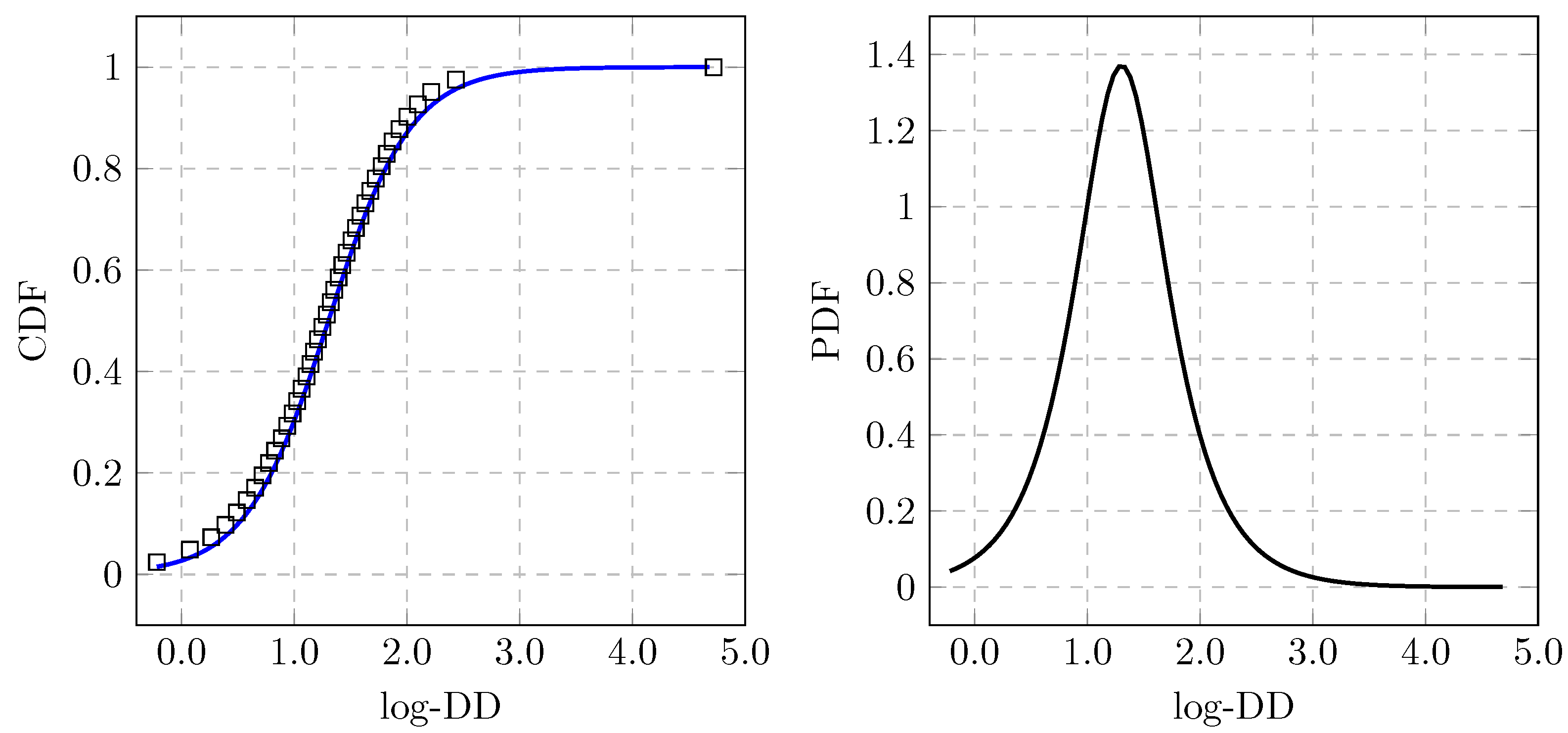
• The empirical distribution of DDs, representing the distribution of the rank variable of the underlying population, is estimated from an empirical sample of DDs.
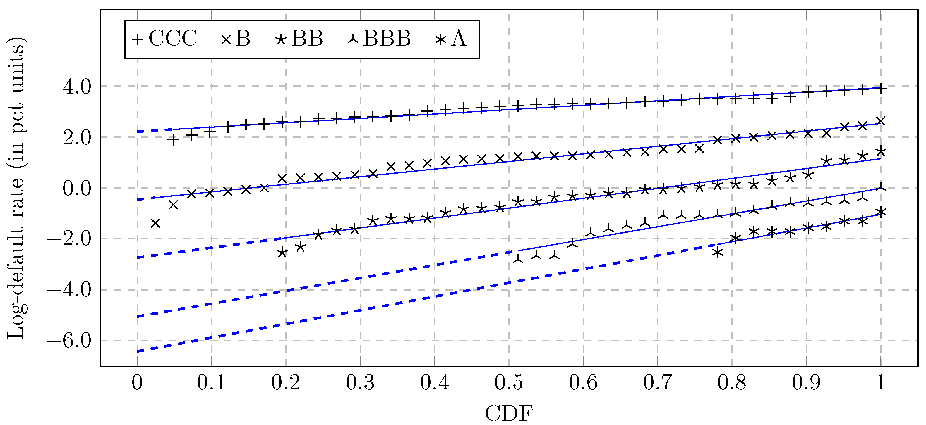
• The empirical distribution of the EDFs is estimated from the summary statistics of historical annual default rates.
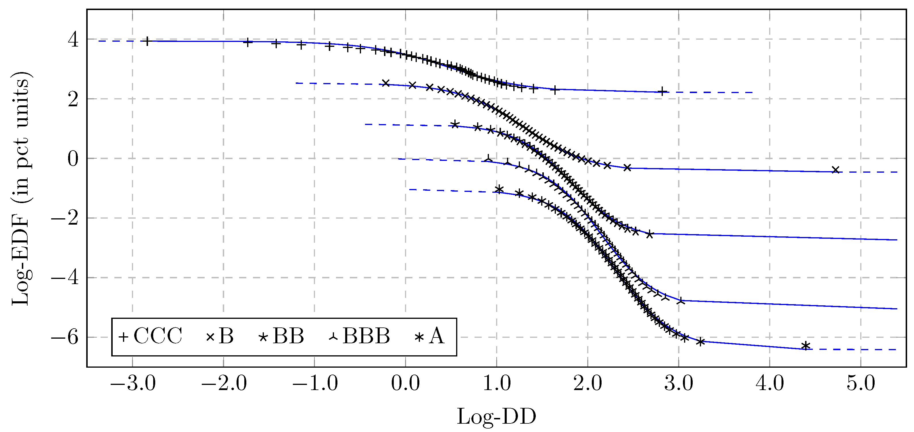
• A quantile matching strategy is applied to establish a relation between DD and EDF. This results in the correspondence $\mathrm{DD}\mapsto \mathrm{EDF}$ as a discrete function with a domain determined by the chosen quantile points in the EDF axis.
• The discrete function from the previous step is approximated using a differentiable function.

It is instructive to ‘invert the axes’ of the usual CDF function by setting the CDF to be the x-coordinate and the EDF the be y-coordinate. The CDF value x in the empirical EDF distribution is replaced with the corresponding $1-x$ quantile of the DD distribution for each distinct x. Then, the resulting discrete relationship is approximated by a differential one. By construction, the DD and EDF dependence holds over the full domain of the empirically observed DDs, i.e., no data reduction along the DD dimension is performed. In addition, because Hypothesis II concerns the EDF directly, there is no need to construct the ETDF as an intermediate step. The quantile matching strategy is common tool, especially in severity modeling. For instance, Albrecher et al. (2017) provides an overview of how to apply this in the case of re-insurance claims.

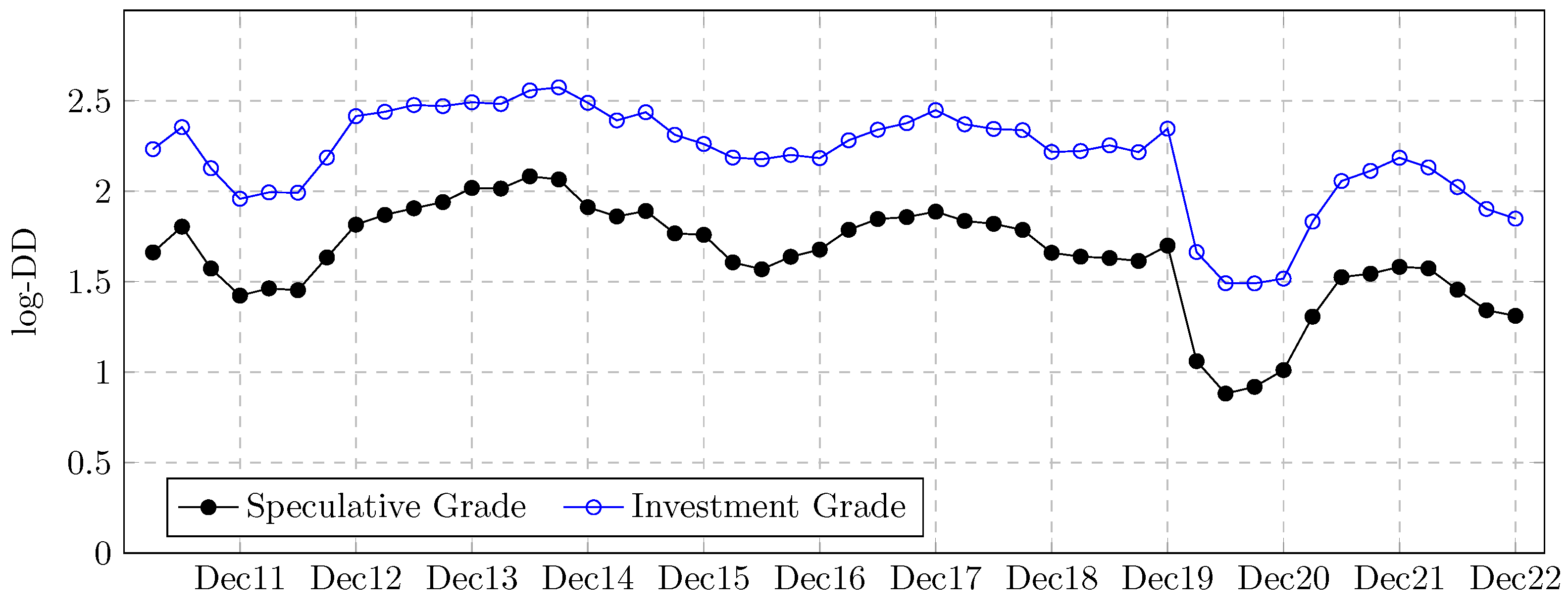
3.2. Distance-to-Default

The DD in (4) is computed over a large panel of corporations at a quarterly frequency. The price and balance sheet data comprise publicly available data from exchanges in North America, South America, Europe, Asia and Australia. The sample contains large-, medium- and small-cap corporations; for instance, the corporations listed in Pink sheets are included. The credit ratings are S&P ratings, which are publicly available from 2010 under SEC Regulation 17g-7.

The sample that we use to represent the population of public corporates consists of 2045 rated corporations between March 2011 and December 2022. In total, there are 54,965 data points.

Table 1. Percentiles of the DD values.

Percentile	CCC	B	BB	BBB	A
5th percentile	0.18	1.10	2.23	3.08	3.52
25th percentile	0.88	2.33	4.15	5.68	6.58
50th percentile	1.62	3.55	5.98	8.44	9.79
75th percentile	2.35	5.28	8.25	11.55	13.68
95th percentile	4.07	9.11	12.45	17.25	21.35

summarizes the percentiles for the DDs in the sample for the investigated rating categories.

The investment grade rating categories that are included are A and BBB, while the speculative grade categories are BB, B, and the CCC category, which comprises all corporations with a rating of CCC or below but does not include corporations that have announced a default (i.e., the D category). It is important to note that there is a good amount of overlap in the DD values between different ratings. For instance, the 75th percentile in CCC, the 25th percentile in B, and the 5th percentile in BB are roughly equivalent.

The time series medians of the log–DD for investment-grade and speculative-grade corporations are depicted in Figure 1.

The average month has a log–DD equal to $2.20$ in the case of investment-grade corporations and $1.65$ in the case of speculative-grade corporations. The values are slightly stressed in 2012 as a result of the European sovereign debt crisis, after which the values increase. In 2015 and 2016 there is a slow decline as a result of the stock market selloff. In 2020, the median DD reaches its lowest point in the dataset as a consequence of the COVID-19 pandemic.

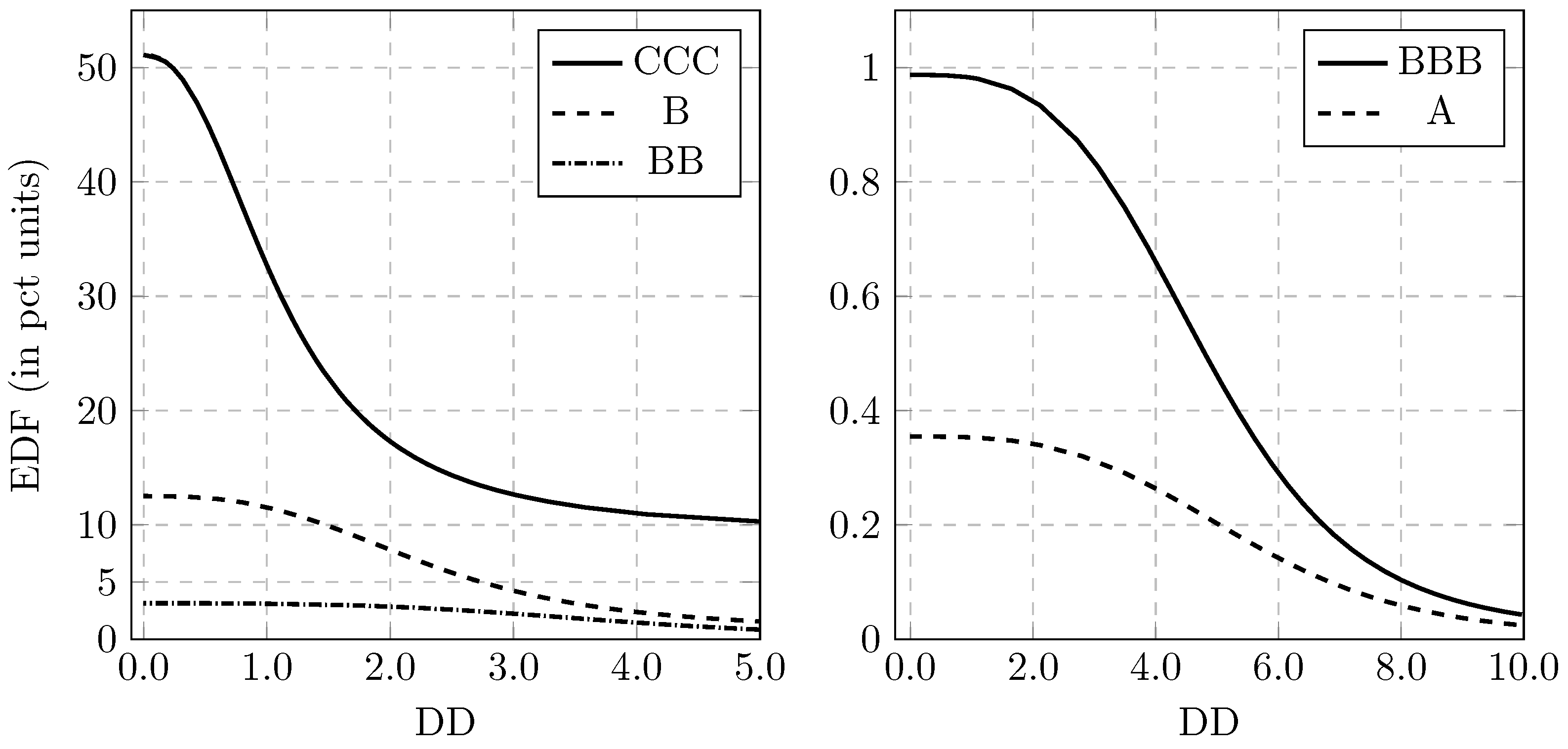
3.3. Expected Default Frequency

The goal of this subsection is to estimate the EDF distributions under Hypothesis II. The mean annual default rates, which are computed by the rating agencies, are the average default frequencies in different calendar years. The annual default rates are computed for different rating categories. Here, we use the S&P summary from Kraemer et al. (2022), where the default rates are computed for the 41 years from 1981 to 2021. We use the same rating categories as in Section 3.2.

Assuming the data reduction formulated in Hypothesis II, we are left with the samples of 41 datapoints in each rating category. Now, we consider the subsamples for each rating category in which the years with default rates of 0 are removed. After ordering these subsamples from the years with the lowest default rates to those with the highest, it can be observed that the log-default rates suggest strong linear dependence. In the CCC and B categories there is just one year with a default rate of 0 (this is 1981, when no CCC corporations defaulted). Naturally, the frequency of such years becomes higher when the rating grows. The years with 0 default rate are problematic, as it is unrealistic to assume that the EDF distribution reaches 0 value.

We approach this by first constructing empirical distribution functions for the sample of log-default rates in each rating category. The 0 values in the default rates formally have a log-default rate value equal to $-\infty$. The steps of the empirical distribution functions are depicted in Figure 2. Next, uniform distribution functions are fitted on the empirical distributions over the domains where the log-default rates have finite values. The line estimator used for this is the mean square error estimator. The solid lines depicted in Figure 2 are the fitted dependencies.

The dashed parts of the regression lines represent the values of the CDF, which are inferred by means of extrapolation over the domains of 0 rates. The resulting EDF distributions are log-uniform distributions. This strategy automatically replaces the zeros in the empirical distribution with nonzero values in the log-uniform distribution. It should be kept in mind that the linear extrapolation is performed in the log-space, and after the transformation to the standard coordinates the zeros are replaced with numbers that are very small compared to the sample means. In fact, the extrapolation has a quite insignificant effect, and the means and variations of the fitted distribution are close to the corresponding values in the empirical distribution. The A category is an exception, as the log-uniform distribution mean overestimates the empirical distribution mean. This is the case because there are very few years with nonzero default rates.

Table 2. Summary of the empirical and fitted log-uniform distributions. The means, standard deviations, and EDF bounds are shown in percentage units.

Variable	CCC	B	BB	BBB	A
Sample mean	24.6	4.09	0.84	0.19	0.05
Fitted mean	24.4	3.99	0.79	0.19	0.07
Sample stdev	11.9	3.25	0.99	0.25	0.10
Fitted stdev	11.8	3.21	0.80	0.24	0.09
${\mathrm{EDF}}^{\downarrow }$	9.12	0.63	0.065	0.006	0.002
${\mathrm{EDF}}^{\uparrow }$	51.1	12.5	3.15	0.99	0.35
$\log \left({\mathrm{EDF}}^{\downarrow }\right)$	2.21	−0.45	−2.74	−5.05	−6.41
$\log \left({\mathrm{EDF}}^{\uparrow }\right)$	3.93	2.52	1.15	−0.013	−1.04
R-squared	0.95	0.94	0.95	0.92	0.87

presents the means and standard deviations of the default rates in the empirical distribution and in the log-uniform distribution, the minimum and maximum default rates in the log-uniform distribution (${\mathrm{EDF}}^{\downarrow }$ and ${\mathrm{EDF}}^{\downarrow }$), and the $R^2$-values.

The log-uniform distributions are referred to as the EDF distributions. They are fully determined by the values ${\mathrm{EDF}}^{\downarrow }$ and ${\mathrm{EDF}}^{\uparrow }$ (or their logarithms). The ETDF associated with the EDF is defined over the uniform domain $[0,1]$ by

$$\begin{array}{c}\hfill \mathrm{ETDF}\left(x\right)=\frac{1}{\beta x}\left(\exp (\alpha +\beta x)-\exp \left(\alpha \right)\right),\end{array}$$

(5)

where $\alpha$ is the intercept and $\beta$ is the slope. The intercept is denoted by $\log \left({\mathrm{EDF}}^{\downarrow }\right)$ in Table 2, while the slope can be recovered by solving $\log \left({\mathrm{EDF}}^{\uparrow }\right)-\log \left({\mathrm{EDF}}^{\downarrow }\right)$. At first sight, the $x\to 0$ limit seems problematic; however, with an application of L’Hopital’s rule, we find that ETDF behaves well around the origin and that the limit is equal to $\exp \left(\alpha \right)$.

The observation that the log–EDF distribution function is well estimated by a linear line is natural. It has been demonstrated by Cappon et al. (2018) that the logarithms of the average default rates computed over several decades are almost perfectly linearly dependent on the credit rating (with the credit ratings considered as numerical values with equal length displacements). Thus, the average default experience grows exponentially worse as the rating declines. Here, we observe that the same is true for a fixed rating in time; the annual average default experience grows exponentially worse with respect to the ranking of the years along the default rates. With Hypothesis II, we move another step forward and assume that this holds for the full population.

3.4. Model Specification

The remaining task is to parse together the DD distribution and the EDF distribution by matching the quantiles. The values x of the log–EDF CDF (the x-coordinate values in Figure 2) are replaced with the $1-x$ quantiles in the empirical log–DD distribution function F. Thus, we impose the relationship

$$\begin{array}{c}\hfill \log \left(\mathrm{EDF}\left(F^{-1}(1-x)\right)\right)=\log \left({\mathrm{EDF}}^{\downarrow }\right)+(\log \left({\mathrm{EDF}}^{\uparrow }\right)-\log \left({\mathrm{EDF}}^{\downarrow }\right))x.\end{array}$$

(6)

Recall that $\log \left({\mathrm{EDF}}^{\uparrow }\right)-\log \left({\mathrm{EDF}}^{\downarrow }\right)$ is the slope for the linear line in Figure 2. The log-coordinates for the DD are used for convenience. We could alternatively apply quantile matching on the empirical DD distribution and then move to the log–DD coordinates, which leads to the same relationship between log–DD and log–EDF, as the quantiles of the empirical log-DD distribution are equal to the logarithms of the quantiles of the empirical DD-distribution.

Figure 3 depicts the relationship from (6) in the log–log space for all of the considered rating categories.

The marks depict the matched quantiles. The lines represent graphs of generalized logistic functions that are fitted on the matched quantiles by minimizing the root mean square error. The solid lines are used over the log–DD values in the empirical sample, while the dashed lines are extrapolated using the fitted generalized logistic functions. In each case, these functions explain the dependence with good accuracy. The generalized logistic functions are defined by

$$\begin{array}{c}\hfill \log \left(\mathrm{EDF}\left(\mathrm{DD}\right)\right)=\log \left({\mathrm{EDF}}^{\uparrow }\right)+\frac{\log \left({\mathrm{EDF}}^{\downarrow }\right)-\log \left({\mathrm{EDF}}^{\uparrow }\right)}{1+e^{Q-B·\log \left(\mathrm{DD}\right)}}.\end{array}$$

(7)

This function is a logistic function with a range that has been transformed to the open interval between ${\mathrm{EDF}}^{\downarrow }$ and ${\mathrm{EDF}}^{\uparrow }$. The fitted parameters are available in

Table 3. Fitted parameters for the generalized logistic functions.

Parameter	CCC	B	BB	BBB	A
Q	1.05	3.58	5.94	6.91	7.15
B	2.27	2.74	3.28	3.22	3.10

and the values of ${\mathrm{EDF}}^{\downarrow }$ and ${\mathrm{EDF}}^{\uparrow }$ in Table 2.

The functional form of the DD–EDF dependence is

$$\mathrm{EDF}\left(\mathrm{DD}\right)={\mathrm{EDF}}^{\uparrow }·\exp \left(\frac{\log \left({\mathrm{EDF}}^{\downarrow }\right)-\log \left({\mathrm{EDF}}^{\uparrow }\right)}{1+e^{Q-B·\log \left(\mathrm{DD}\right)}}\right).$$

The EDF curves stabilize towards the minimum EDFs over the tails with increasing DDs. The EDFs are strongly positive-sloping (in relative terms) as the DD shortens, and they stabilize towards the maximum values. The regions of steep sloping are rating-dependent. This behaviour is depicted in Figure 4.

At any point in the DD axis, the predicted EDF values are with respect to the credit ratings; a higher EDF is always assigned in a case with a lower rating. Under rating transitions, a new inference about the default risk can be made based on the DD value and the newly selected EDF curve. In this respect, the model behavior is similar to the spread risk model based on credit spread curves.

Table 4. Summary of selected EDF values, means, and standard deviations in percentage units.

Rating	High-Limit	DD 1	DD 2	DD 4	DD 6	DD 8	DD 10	Low-Limit	Mean	Stdev
CCC	51.1	33.2	17.4	11.0	9.86	9.50	9.35	9.12	24.4	11.8
B	12.5	11.5	7.82	2.38	1.18	0.87	0.76	0.63	3.99	3.21
BB	3.15	3.12	2.86	1.46	0.48	0.20	0.12	0.06	0.79	0.80
BBB	0.99	0.98	0.94	0.66	0.29	0.10	0.04	0.006	0.19	0.24
A	0.35	0.35	0.34	0.26	0.14	0.06	0.02	0.002	0.07	0.09

presents the EDF values for various DDs, the low and high limits of the EDFs, the means, and the standard deviations.

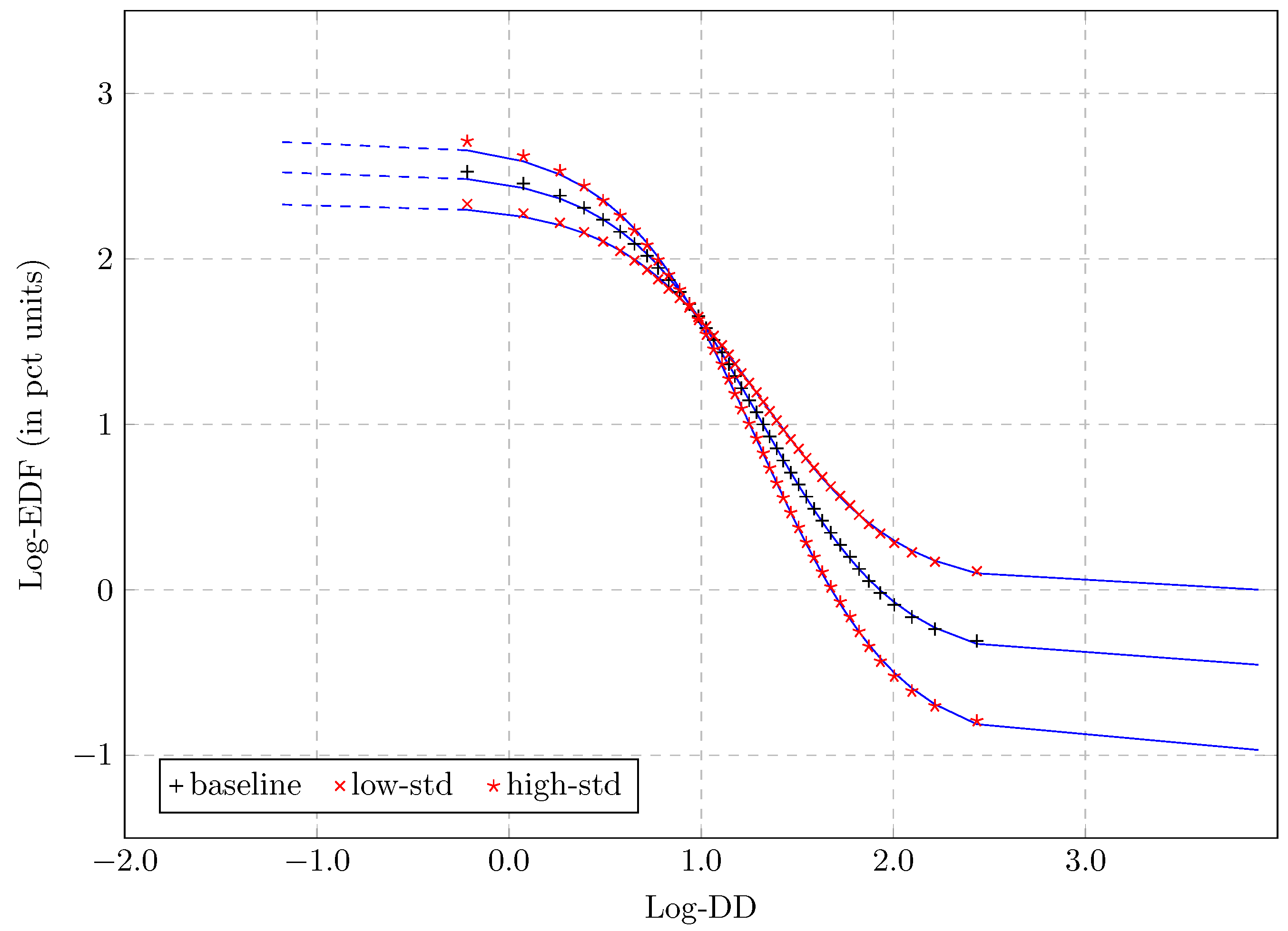
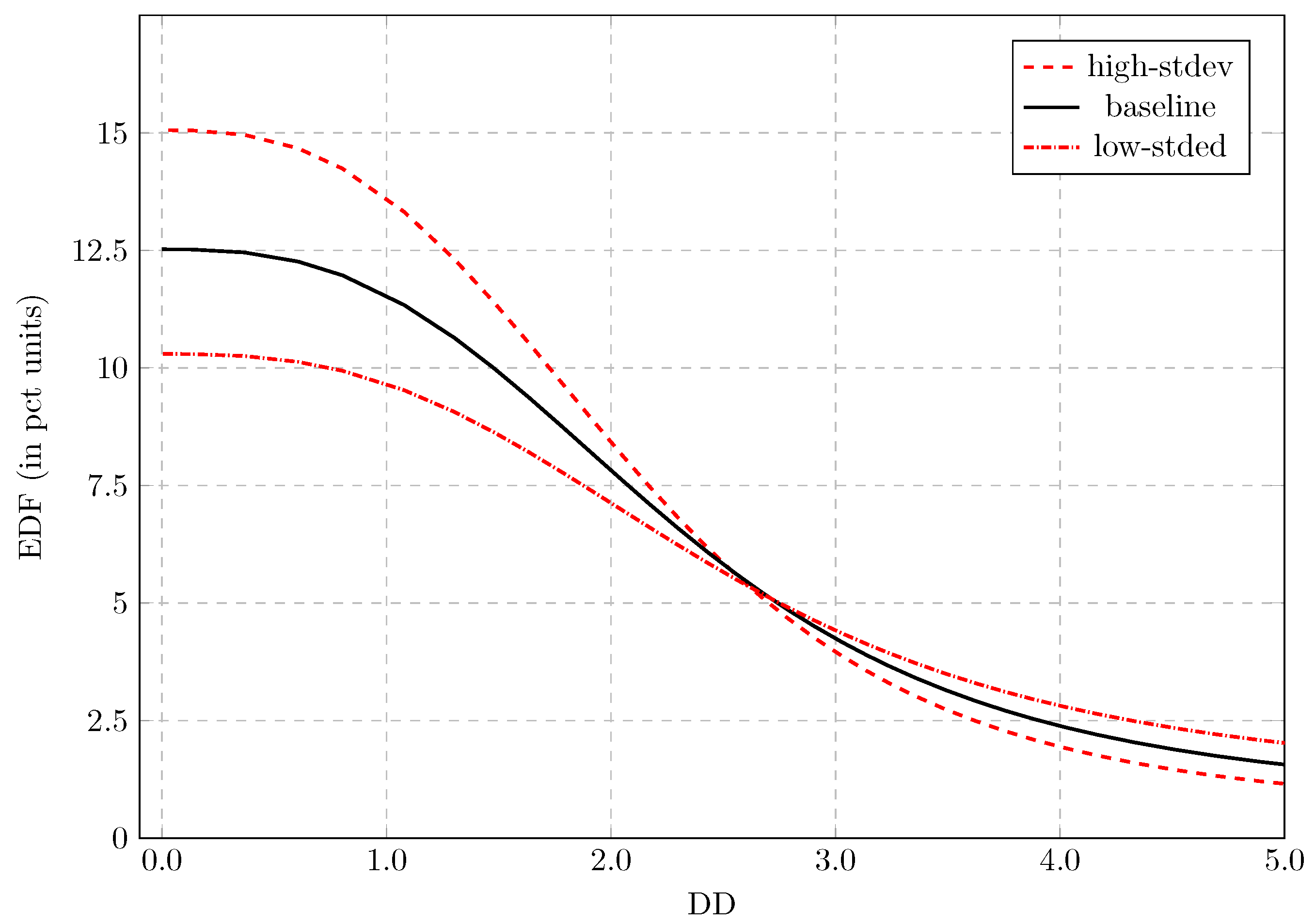
3.5. Sensitivity to the Parameters

In Section 3.3, we argued that the EDFs have a log-uniform distribution. This was obtained through an analysis of annual default rate summaries, which was justified by Hypothesis II. The resulting EDF had a mean close to the average empirical default rate. In the following analysis, we alter the parameters of the linear functions explaining the log-EDF distributions depicted in Figure 2. Specifically, we investigate how the relation between the log–EDF and log–DD behave under such changes. The parameters of the linear dependencies are shifted such that the EDF mean remains fixed while the variation changes. The uniform distribution for the log–EDF is specified by the bounds $\log \left({\mathrm{EDF}}^{\downarrow }\right)$ and $\log \left({\mathrm{EDF}}^{\uparrow }\right)$. It seems natural to widen (or narrow) these bounds by the same constant x from both sides. This, however, alters the mean of the EDFs. We can stabilize the mean by shifting the new bounds by another constant s determined in such a way as to keep the mean EDF static. Thus, here we are using a transformation of type

$$\begin{array}{c}\hfill \log \left({\mathrm{EDF}}^{\downarrow }\right)\mapsto \log \left({\mathrm{EDF}}^{\downarrow }\right)-x+s\mathrm{and}\log \left({\mathrm{EDF}}^{\uparrow }\right)\mapsto \log \left({\mathrm{EDF}}^{\uparrow }\right)+x+s,\end{array}$$

where $x>0$ if we widen the bounds (i.e., increase the variance) and $x<0$ if we narrow the bounds (i.e., decrease the variance).

In the following, we focus on the B-rating category. We can choose to shift the value x (and adjust s to keep the mean static) as long as we reach an increase in the standard deviation of the EDF by $20\%$, then do the same to achieve a decrease in the standard deviation by $-20\%$. The parameter values are $x=0.35$, $s=-0.17$ in the former case and $x=-0.33$ and $s=0.13$ in the latter. Figure 5 presents how this influences the points chosen for quantile matching.

The lines in Figure 5 are graphs of generalized logistic functions with parameters estimated by minimizing the root mean square error between the quantile matching points and the logistic function. The parameters, means, and standard deviations of the EDF are presented in

Table 5. Summary of model implied statistics and model parameters (B-category).

Hypothesis	Mean	Stdev	Rel-Stdev	Q	B	${\mathbf{EDF}}^{\downarrow }$	${\mathbf{EDF}}^{\uparrow }$
Low-stdev	3.99	2.57	$0.8\sigma$	3.58	2.74	1.00	10.3
Baseline	3.99	3.21	$\sigma$	3.58	2.74	0.63	12.5
High-stdev	3.99	3.86	$1.2\sigma$	3.58	2.74	0.38	15.1

.

The DD–EDF relationships in the standard coordinates are depicted in Figure 6.

Table 5 suggest first that the EDF mean is invariant under the shifts (which is controlled), and second that the parameters B and Q are invariant. Why is this the case? In the relation from (6), we can write $F^{-1}(1-x)=F\log \left(\mathrm{DD}\right)$ and $1-x=F\left(\log \right(\mathrm{DD}\left)\right)$, which results in

$$\begin{array}{ccc}\hfill \log \left(\mathrm{EDF}\right(\mathrm{DD}\left)\right)& =& \log \left({\mathrm{EDF}}^{\downarrow }\right)+(\log \left({\mathrm{EDF}}^{\uparrow }\right)-\log \left({\mathrm{EDF}}^{\downarrow }\right))(1-F\left(\log \left(\mathrm{DD}\right)\right))\hfill \\ & =& \log \left({\mathrm{EDF}}^{\uparrow }\right)+(\log \left({\mathrm{EDF}}^{\downarrow }\right)-\log \left({\mathrm{EDF}}^{\uparrow }\right))F\left(\log \left(\mathrm{DD}\right)\right)\hfill \end{array}$$

(8)

where F is the empirical log–DD distribution. Now, the sum of square errors in fitting the parameters Q and B in (7) to this function over the quantile matching points is proportional to the square of $\log \left({\mathrm{EDF}}^{\uparrow }\right)-\log \left({\mathrm{EDF}}^{\downarrow }\right)$ and to the sum of square errors when matching the logistic function $1/(1+\exp (Q-B·\log \left(\mathrm{DD}\right)\left)\right)$ to $F\left(\log \right(\mathrm{DD}\left)\right)$. Only the latter component has dependence on Q and B. The latter component does not have dependence on the EDF distribution, and is fully derived using the DD sample. Therefore, the optimal values for B and Q are not dependent on $\log \left({\mathrm{EDF}}^{\uparrow }\right)$ or $\log \left({\mathrm{EDF}}^{\downarrow }\right)$. Another interesting remark here is that the log–DD sample is well explained by a logistic distribution in each rating category. In the standard notation, the CDF and PDF of the logistic distributions are defined by

$$\begin{array}{c}\hfill L\left(x\right)=\frac{1}{1+\exp (-(x-\mu )/s)}\mathrm{and}l\left(x\right)=\frac{\exp (-(x-\mu )/s)}{s{(1+\exp (-(x-\mu )/s))}^2}\end{array}$$

where $\mu =Q/B$ and $s=1/B$. Figure 7 depicts the CDF and PDF for the B-category. The marks in the CDF plot are empirical distribution values.

The respective maximum absolute distances between the empirical log–DD distribution and the logistic approximation are $0.04$, $0.04$, $0.04$, $0.03$, and $0.07$ for the categories A, BBB, BB, B, and CCC.

Based on the observations made in this subsection, Hypothesis II can be relaxed without altering the model specification. The assumption that the log–EDF distribution is linear, with unknown parameters ${\mathrm{EDF}}^{\downarrow }$ and ${\mathrm{EDF}}^{\uparrow }$, leads to a generalized logistic dependency between log–DD and log–EDF in an EDF model of public corporations based on the DD rank estimator. Thus, under the linear hypothesis concerning the log–EDF distribution, it is only necessary to address the following problem:

• How can the minimum and maximum EDFs in each rating category be determined?

4. Discussion

The conventional method for modeling the EDFs often entails using agency credit ratings as a measure of entity credit quality and assigning historical average default rates to each rating in order to establish the EDFs. Another common strategy is to make a parametric inference about the EDFs, often assuming that the EDF is a logistic function of a credit quality variable. These considerations prompt us to pose the following question: How is it possible to systematically explain the EDFs without relying on strong parametric assumptions about the EDF function? We propose that the problem of finding the EDF function can be divided into two separate steps. The first problem, which can be solved independently of the second, involves identifying the credit rank variable. The rank estimator seeks a variable that ranks entities from the most vulnerable to default to the least vulnerable. The second step requires a non-parametric strategy for estimating the EDF dependency on the chosen rank variable. In the estimation of the EDF, we introduce a new variable called ETDF, which offers the advantage of accommodating larger sample sizes than the typical EDF estimator. The resulting ETDF is a discrete function of the rank variable. The EDF is related to the ETDF through an integral equation. To solve for the EDF, the ETDF must be approximated using a differentiable function. This approximation entails selecting a function from the space of all differentiable functions, which requires a certain degree of judgment, which this is where the non-parametric inference is required.

The second part of this study delves into a model that can be considered a prototype within the framework outlined earlier. The entities under consideration are public corporations. This choice is very convenient for studying this paradigm, as many studies have concluded from empirical analysis that the DD variable is a strong candidate for the rank variable. We then argue that, for each credit rating category, the EDF can be represented as an exponential function over a uniform sample that is ordered by credit quality. In other words, over a uniform domain, the expected default experience grows exponentially worse as the credit quality of the issuer decreases. This concept finds support in the time series behavior of historical default rates, allowing the EDF over the uniform sample to be inferred from the default rate summaries. It is often easier to work with the linear functions, and as such we represent the log–EDF as a function that increases linearly as the credit quality improves. Next, we apply the hypothesis that the DD has the ability to rank the sample in credit quality, which allows us to use quantile matching and present the log–EDF as a discrete function of the DD. However, it turns out that it is easier to approximate the log–EDF with a differentiable function when the log–DD is used as the rank variable (note that $\log \left(\mathrm{DD}\right)$ and DD rank the sample accordingly). Through data visualization and a trial-and-error approach, it was found that the dependence between log–DD and log–EDF can be approximated accurately using the generalized logistic functions. The EDF function of the DD is presented in (8). The ETDF associated with this model is presented in (5). This prototype model has convenient properties. For instance, we have noted that to specify the EDF function it is sufficient to first determine two parameters (the upper and lower EDF limits), then solve the remaining parameters by estimating the logistic distribution for the log–DDs.

The idea of separating the task of finding the rank variable from the estimation of the EDF function is known from the KMV approach to EDF modeling, as discussed by Kealhofer (2003a) and Duffie and Singleton (2003). However, the details on the DD and the EDF function in these papers have not not published. In this study, we propose a non-parametric strategy to find the EDF function. The prototype model outlined earlier paves the way for a novel form of inference concerning EDFs. This specification differs from the usual parametric models used in credit risk modeling, such as the logistic and hazard rate models (as seen in the works of Chava and Jarrow (2004) and Campbell et al. (2008)), as well as structural models such as Gordy and Heitfield (2001). In the latter case, the EDF is typically represented as a normal distribution function (sometimes a fat-tailed distribution function) of the rank variable. The logistic models assume that the EDF itself can be explained as a logistic function of some covariates. Here, we argue that the log–EDF can be explained as a generalized logistic function of the log–DD. The logistic function in this relation arises because the log–DD distribution can be explained using the logistic distribution.

The primary limitation of this study lies in the small dataset used for the prototype model. This limitation led us to formulate a hypothesis regarding the EDFs rather than estimating the frequencies on the issuer level empirical default experience data. In a more expansive empirical study, it would be possible to estimate the ETDF by initially fitting the empirical ETDFs over the uniform domain using the estimator defined in (3). Subsequently, the parameters of the ETDFs associated with the log-uniform model could be fitted to these empirical ETDFs using (5). Another limitation to note is that this study did not introduce an out-of-sample test to assess performance.

A potential extension of the prototype model could involve estimating the expected credit rating transition frequencies for public corporates using DD as the rank variable. Now, the same inferences about the expected credit transition frequencies can be made as in the analysis of defaults above. In particular, to estimate the model over the uniform domain one would estimate the parameters of the expected tail frequency using the straightforward modification of (3) for the transition frequencies, followed by finding the model parameters by fitting (5). The associated expected transition frequency can be explained with the exponential function. The expected transition frequency as a function of DD has the same specification as (8), where F is the distribution function of the $\log \left(\mathrm{DD}\right)$s. Beyond public corporations, this strategy to estimate the EDF can be used to estimate the expected frequencies of other credit events and to estimate credit event-related frequencies for non-corporate issuers. A metric similar to DD has been used to analyze the credit risk of sovereign entities. The framework introduced in this manuscript could potentially be used to analyze EDFs in this domain as well.

5. Conclusions

In this paper, we have introduced a generic modeling strategy for EDFs. This strategy consist of two steps: first, a rank variable is selected which allows for ranking the bond issuer entities from the most likely to default to the least likely; second, the EDF can be recovered by fitting the ETDF on the ranked sample, then solving a simple integral equation for the EDF. The remainder of the manuscript produces details of prototype models for the EDFs of public corporations across multiple rating categories. In this prototype, a data reduction hypothesis regarding the EDFs has been put in place, leading to the inference that the EDF distribution is log-uniform. We found by studying the time series of historical default rates that the log-uniform distribution for the EDFs seems very reasonable. In a subsequent step, we found that if we explain the variation of the EDFs using the DDs, this leads to a generalized logistic function dependency between the log–DD and log–EDF. We further analyzed the sample of DDs and found that the reason that the quantile matching strategy gives rise to an approximate logistic dependency is that the empirical DD distributions are well approximated by the logistic distributions. In addition, we introduce the estimators needed to fit this prototype model.

References

1. Albrecher, Hansjörg, Jan Beirlant, and Jozef L. Teugels. 2017. Reinsurance: Actuarial and Statistical Aspects. Statistics in Practice. Hoboken: John Wiley & Sons. [Google Scholar]
2. Berndt, Antje, Rohan Douglas, Darrell Duffie, and Mark Ferguson. 2018. Corporate credit risk premia. Review of Finance 22: 419–54. [Google Scholar] [CrossRef]
3. Bharath, Sreedhar T., and Tyler Shumway. 2008. Forecasting default with the Merton distance to default model. Review of Financial Studies 21: 1339–69. [Google Scholar] [CrossRef]
4. Bohn, Jeffrey R. 2000. An empirical assessment of a simple contingent-claims model for the valuation of risky debt. The Journal of Risk Finance 1: 55–77. [Google Scholar] [CrossRef]
5. Campbell, John Y., Jens Hilscher, and Jan Szilagyi. 2008. In search of distress risk. The Journal of Finance 63: 2899–939. [Google Scholar] [CrossRef]
6. Cappon, Andre, Alexander Gorenstein, Stephan Mignot, and Guy Manuel. 2018. Credit ratings, default probabilities, and logarithms. The Journal of Structure Finance 24: 39–49. [Google Scholar] [CrossRef]
7. Chava, Sudheer, and Robert A. Jarrow. 2004. Bankruptcy prediction with industry effects. Review of Finance 8: 537–69. [Google Scholar] [CrossRef]
8. Crouhy, Michel, Dan Galai, and Robert Mark. 2000. A comparative analysis of current credit risk models. Journal of Banking & Finance 24: 59–117. [Google Scholar] [CrossRef]
9. Denzler, Stefan M., Michel M. Dacorogna, Ulrich A. Müller, and Alexander J. McNeil. 2006. From default probabilities to credit spreads: Credit risk models do explain market prices. Finance Research Letters 3: 79–95. [Google Scholar] [CrossRef]
10. Duffie, Darrell, and Kenneth J. Singleton. 2003. Credit Risk. Princeton: Princeton University Press. [Google Scholar]
11. Frey, Rüdiger, and Alexander J. McNeil. 2003. Dependent defaults in models of portfolio credit risk. Journal of Risk 6: 59–92. [Google Scholar] [CrossRef]
12. Gapen, Michael, Dale Gray, Cheng Hoon Lim, and Yingbin Xiao. 2008. Measuring and analyzing sovereign risk with contingent claims. IMF Staff Papers 55: 109–48. [Google Scholar] [CrossRef]
13. Gordy, Michael, and Erik Heitfield. 2001. Of Moody’s and Merton: A Structural Model of Bond Rating Transitions, Technical Report; Federal Reserve.
14. Gray, Dale F., Robert C. Merton, and Zvi Bodie. 2007. Contingent claims approach to measuring and managing sovereign credit risk. Journal of Investment Management 5: 5–28. [Google Scholar] [CrossRef]
15. Gupton, Greg M., Christopther C. Finger, and Mickey Bhatia. 1997. Creditmetrics. Technical Report. New York: J. P. Morgan. [Google Scholar]
16. Harju, Antti J. 2013. Edf-Rank-Estimator. Available online: https://github.com/harju-aj/edf-rank-estimator (accessed on 1 October 2023).
17. Hull, John C., and Alan White. 2000. Valuing credit default swaps I: No counterparty default risk. Journal of Derivatives 8: 29–40. [Google Scholar] [CrossRef]
18. Jessen, Cathrine, and David Lando. 2015. Robustness of distance-to-default. Journal of Banking & Finance 50: 493–505. [Google Scholar] [CrossRef]
19. Kealhofer, Stephen. 2003a. Quantifying credit risk I: Default prediction. Financial Analyst Journal 59: 30–44. [Google Scholar] [CrossRef]
20. Kealhofer, Stephen. 2003b. Quantifying credit risk II: Debt valuation. Financial Analysts Journal 59: 78–92. [Google Scholar] [CrossRef]
21. Kraemer, N. W., J. Palmer, M. R. Nivritti, I. Sundaram, F. Lyndon, and M. Abinash. 2022. Default, Transition, and Recovery: 2021 Annual Global Corporate Default and Rating Transition Study, Technical Report. S&P Global.
22. McNeil, Alexander J., Rüdiger Frey, and Paul Embrechts. 2005. Quantitative Risk Management—Concepts, Techniques and Tools. Princeton: Princeton University Press. [Google Scholar]
23. Merton, Robert C. 1974. On the pricing of corporate debt: The risk structure of interest rates. Journal of Finance 29: 449–70. [Google Scholar] [CrossRef]
24. Stephanou, Constantinos, and Juan Carlos Mendoza. 2005. Credit Risk Measurement under Basel II: An Overview and Implementation Issues for Developing Countries. World Bank Policy Research Working Paper 3556. Washington, DC: World Bank. [Google Scholar]
25. Vassalou, Maria, and Yuhang Xing. 2004. Default risk in equity returns. Journal of Finance 59: 831–68. [Google Scholar] [CrossRef]
26. Zhang, Benjamin Yibin, Hao Zhou, and Haibin Zhu. 2009. Explaining credit default swap spreads with the equity volatility and jump risks of individual firms. Review of Financial Studies 22: 5099–131. [Google Scholar] [CrossRef]
Figure 1. Median log–DD time series.
Jrfm 16 00444 g001
Figure 2. Expected default frequencies.
Jrfm 16 00444 g002
Figure 3. Relationship between log–DD and log–EDF.
Jrfm 16 00444 g003
Figure 4. Relationship between DD and EDF.
Jrfm 16 00444 g004
Figure 5. B-category log–DD and log–EDF dependencies.
Jrfm 16 00444 g005
Figure 6. B-category DD and EDF dependencies.
Jrfm 16 00444 g006
Figure 7. CDF and PDF functions for the logistic distribution of log–DDs in B category.
Jrfm 16 00444 g007