Abstract
Typically, the explanatory variables included in a regression model, in conjunction with the omitted relevant regressors implied by the usual error term, have both direct and indirect effects on the dependent variable. Attempts to obtain their separate estimates have been plagued with simultaneity issues. To circumvent these problems, this paper defines their sum as “total effects”, develops a time-varying coefficients methodology for their estimation without simultaneity bias, and applies these techniques to estimate the total effects of commercial bank credit per-capita on real GDP per-capita in Mauritius. An innovation is the introduction of extraneous variables that act as “coefficient drivers” chosen on the basis of best predictive performance, as measured by the smallest value of Theil’s U-statistic we were able to locate in the estimation.
1. Introduction
As is—or should be—known from Pratt and Schlaifer (1984), every regressor included in a regression equation has both direct and indirect effects on its dependent variable. In contrast to traditional econometric practice, which side-steps the issue of indirect effects, we shall follow Pratt and Schlaifer (1984) and account for such direct and indirect effects by estimating their sum as “total effects.” Since it is unlikely in most economic settings that the total effects of a given regressor are constant, we generalize the proposed model, by allowing all of its coefficients to be time-varying, necessitating the use of “modified generalized least squares.”1 Recognizing that available data for the variables included in our model do not contain sufficient information about the indirect effects of the regressor of our model, we shall utilize additional information over and above the information already contained in the specified variables of the model by introducing so-called “coefficient drivers” without knowing whether this additional information is relevant or not. These coefficient drivers are variables not actually included in the set of regressors but having an influence on how the coefficients associated with regressors impact the dependent variable over time. As a consequence, the coefficients themselves become functions of coefficient drivers not otherwise in a model but, nevertheless, playing important roles in how the dependent variable responds to its regressors over time. The choice of such variables is inductive and should be guided by empiricism which we advocate using Theil’s U-statistic, a measure of predictive performance that is invariant to scaling, rather than a Neyman–Pearson test criterion, to improve the accuracy of results. In all this, we were motivated by a desire to obtain results that are as precise and empirically relevant as feasible.
The remaining part of this paper is divided into six sections. Section 2 provides the motivation for the model to be estimated and gives an economic background. In Section 3, we develop a model with time-varying coefficients. The novelty of this model is that the coefficient on the regressor included in a regression equation measures the regressor’s total effect on the dependent variable. Section 4 gives some implications of the model developed in Section 3 for the relationship between economic growth and financial development. Section 5 is concerned with the estimation of the total effect of commercial bank credit (CBC) on real gross domestic (RGDP) for the period 1970–2019 in Mauritius. Section 6 offers a detailed rationale for our choice of, and need for, estimating a model with time-varying coefficients. Section 7 concludes.
2. The Economic Background
Early economists, such as Bagehot (1873) and Schumpeter (1912), suggested that finance leads to economic development. More recent theory on finance and endogenous growth likewise suggest that more finance can have a positive effect on economic growth; Greenwood and Jovanovic (1990); Pagano (1993); King and Levine (1993); Berthelemy and Varoudakis (1996). However, the empirical literature has found mixed evidence of the effects of finance on growth. A comprehensive review by Levine (2005) found that more finance tends to be beneficial to the economy, so that countries with a smaller share of credit to GDP should attempt to increase it to promote investment and growth. In general, the empirical literature is ambiguous in its conclusions, suggesting a diminishing-returns non-linear relationship between “financial deepening” and economic growth, in that too much finance might be harmful for growth (see Deidda and Fattouh 2002; Huang and Lin 2009; Arcand et al. 2012, 2015; Cecchetti and Kharroubi 2012, 2013; Law and Singh 2014).
In the case of Mauritius, empirical studies on finance and growth have generally found a positive link between GDP (or investment or economic growth) and different quantitative measures of financial development (FD), such as the ratio of liquid liabilities of banks to GDP, and private sector credit (see Jouan 2005; Jankee 2006; Seetanah 2008; Nowbutsing et al. 2010; Muyambiri and Odhiambo 2018). None of these studies considered the possibility of the time-variability of the total effects of finance on growth. To pursue this possibility, this paper applies a time-varying coefficient (TVC) model to explore how the relationship between financial development and economic growth in Mauritius may have changed over time, possibly as a consequence of changes in economic policies and structural economic changes in the country since independence in 1968. In contrast to existing fixed and variable coefficient models,2 which ignore the indirect effects of the regressor on the dependent variable, the TVC model of Swamy and von zur Muehlen (2020) measures the total effects of bank credit on RGDP from 1970 to 2019.
In this paper, we focus on total bank credit as a measure of financial development, because the transaction activities of a commercial bank are different from those of other financial intermediaries, such as an insurance company, in that the former, when transacting with the latter, discharges its payment obligations to the latter by issuing deposits, whereas when agents belonging to the latter group transact with each other, they do so by transferring existing deposits. When an insurance company lends to a household, it pays by transferring money it holds with a bank (an asset to the insurance company), thereby leaving the total stock of money unaffected. In contrast, when the bank extends a loan to a household, it discharges its obligation to pay by crediting the household’s account, thereby increasing the total stock of money (See Werner 2005).
The theoretical background of and interest in the potential role of bank credit in promoting GDP is the literature inaugurated by Werner (1992), who argued that in order for GDP to expand, more money is needed to settle those transactions, implying that when banks create money, credit, and new purchasing power, they contribute to GDP not merely sectorally but, more importantly, to the expansion of GDP as a whole. Werner (2012) argued that it is the portion of bank credit allocated to GDP-type spending as opposed to financial transactions that drives GDP. If this conjecture is correct, we should expect a diminishing effect of total bank credit on GDP over time if bank credit in Mauritius underwent shifts from real to financial spending. In this paper, we focus on the effects of bank credit on RGDP.
3. A Model with Time-Varying Coefficients
In this section, we describe a relationship between per-capita RGDP and per-capita CBC utilizing time-varying coefficients and carefully selected coefficient drivers, particularly to improve predictive performance, where, importantly, these time-varying coefficients are to be taken as random variables. We assert that the total effect of per-capita = per-capita CBC on per-capita = RGDP per-capita can be cast in terms of two relationships, as follows:
First, is related to plus an unspecified set of excluded relevant variables, denoted , via the following relation with time-varying coefficients, based on the methodology introduced by Swamy and Tinsley (1980),
where Wt contains the effects of excluded relevant variables. Here is written as a scalar and not potentially a vector, as done by Pratt and Schlaifer (1984).
Second, recognizing that Equation (1) suffers from a simultaneity problem caused by the correlation of with , Pratt and Schlaifer (1984) proposed augmenting (1) with the stochastic relationship,
where is a random error term and i.i.d. (0, ).
Our contribution is (1) the introduction of time-varying coefficients that (2) are potentially driven by variables not otherwise part of the model.
Substituting the right-hand side of Equation (2) for in Equation (1), gives
where , which is i.i.d. (0, ), is the error term of Equation (3), coefficient is the direct and the term represents the indirect effect of on .3 This indirect effect arises because affects as in (2), and affects as in (1). The sum of these direct and indirect effects, ( + ), is the total effect of on alluded to in the Introduction.
Pratt and Schlaifer (1984) claim that while the direct effect and the indirect effect are non-unique, their sum ( + ), called the total effect, is unique. To prove that the total effect is unique, we need to show in how many ways the total effect can be non-unique and how we can avoid all these ways. As such, in order to avoid issues in proving the uniqueness of total effects, we chose to write the effects of excluded relevant regressors in terms of a scalar , compared with Pratt and Schlaifer (1984)4, who write this as the product of two vectors.5
Note that Equation (3) is free from simultaneity problems because is independent of . The case for estimating total effects is further strengthened when one considers two principal defects of models such as the widely used Kalman filter (Durbin and Koopman 2001): their lack of an i.i.d. error term and their inability to measure the indirect effects of regressors.
To proceed, re-write the relationship between and as
where = ( + ) and = ( + ) = the total effect of on .
In vector form
where = (1 ) is a 1 2 vector, = ( a 2 1 vector, and from now on all vectors are denoted by bold symbols. The sample information is ( ), t = 1, 2, …, T.
As is evident from (1), the information contained in data on and is adequate to estimate direct effects with precision, but it may not be enough to estimate indirect effects. Therefore, as promised in the Introduction, we now consider additional observable variables that hopefully contain information about . Since we do not know a priori what information any of these variables may contain, we use a heuristic approach of experimenting with various candidates that look promising from a theoretical point of view. We call them coefficient drivers because of the manner in which we shall use them. Consider two such variables, labelled and , and posit the following two relationships:
Using appropriate matrix algebraic notation, Equations (5) and (6) can be combined into the following single equation:
where is defined in the equation below (4), = is a 2 3 matrix with exclusion restrictions, = (1 is a 3 × 1 vector, and = is a 2 1 vector.
Note that the assumption of time-variability is key: Equations (5) and (6) would be impossible had we treated the coefficients of (4) as constant parameters. Equations (5) and (6) are new to our time-varying coefficients model. Later, we will check systematically what, if any, information is contained in these coefficient drivers.
The coefficients of Equations (5) and (6) have further useful interpretations. The coefficient in Equation (5) is equal to ( + ) where is random. The coefficient driver simply acts as an explanatory variable of . When (5) and (6) are inserted into (4), all the terms on the right-hand side of (6) get multiplied by . Therefore, (i) as the coefficient on can absorb at least part of the direct-effect component of , and (ii) becomes the coefficient on the interaction between and . Such a coefficient cannot absorb the direct-effect component of , but its estimate can indicate whether absorbs at least a part of the indirect-effect component of . Therefore, the estimate of the coefficient π1j reveals the strength or weakness of the relationship between the indirect-effect component of and . If the intercept of (6) does not completely absorb the direct-effect component, and if of the same equation does not completely absorb the indirect-effect component of , then the term corrects the inaccuracies in both, if the equality sign of (6) holds.
The sample information and the additional information can be combined by substituting the right-hand side of the equation = + , for in Equation (4). Doing so gives = + = () + ut where denotes the Kronecker product and is the column stack of .
Stacking the equations = = + , t = 1, 2, …, T, gives = + , where is a T 1 vector of observations on , is a matrix of observations on (), = , = , is a T 1 vector of errors, is a T 2T diagonal matrix with , , …, along the diagonal, and is a 2T 1 vector of the errors of equation which is below Equation (6) for t = 1, 2, …, T.
In addition to (4)–(6), we assume that
where is diagonal with ϕ00 and as its diagonal elements, E = 0 and E = . This assumption of diagonal Φ is required for convergence, because our estimation procedure of the model in (4)–(7) is an iterative procedure.
If the variance–covariance matrix of the error vector of Equation = is denoted by , then the variance-covariance matrix of can be shown to be .
The exclusion restrictions imposed on can be written as = + 0. Combining this equation with = + gives = + where = (y )′, = ( , and = ( 0. The variance–covariance matrix of is singular.
Since the coefficients of (5) and (6) are fixed parameters, they possess consistent estimators. We can find them by applying Paige’s (1979) numerically stable algorithm for the generalized least squares method to equation = + . We also find feasible generalized least squares estimators of , see Swamy (1990). From these estimates, we derive the estimates of using = , as in Swamy (1990). Since the coefficients of Equation (4) are time-varying, they themselves do not possess consistent estimators. However, substituting the above estimates of and , and the data on and on the right hand sides of (5) and (6), respectively, gives the estimates of γ0t and , t = 1, …, T. In other words, given data on and , we find the estimates of , and from their consistent estimators obtained above and the derived estimates of and from = , to obtain the estimates of and from Equations (5) and (6), respectively. However, we do not know the statistical properties of these estimates.
Since is unknown, we use its estimate in its place. Let denote its estimate. The Cholesky factorization of can be represented by . We denote the Cholesky factorization of as . Paige’s (1979) algorithm for performing the generalized least squares estimation can be directly applied to = + .
After this estimation, we find the feasible version of the generalized least squares estimator of ’s by replacing by . The vector is replaced by its estimates. We substitute these feasible versions in place of the unknown coefficients and error terms in Equations (5) and (6), respectively. In conjunction with our data on coefficient drivers, the feasible estimates of and in (5) and (6) give the estimates of ’s and ’s. These estimates are also substituted into Equation (4). The consistency properties of the feasible generalized least squares estimators of fixed coefficients are known in the econometrics literature. The consistency of generalized least squares estimators of are well defined but not of the time-varying coefficients. The only thing we can claim is that the estimates of time-varying coefficients are those implied by the consistent estimators of fixed coefficients.6
4. Implications of the Model of above Section for the Relationship between Economic Growth and Financial Development
Differencing both sides of each of Equations (4)–(6) gives
where is the difference operator, and = − , = + Δu0t, = + , and the vector (, ) is completely unknown.
In the next section, we will be using the model in (4)–(7) to estimate the total effects of CBC per capita on RGDP per capita and, therefore, Equation (8) is nothing but an implication of our model. Dividing both sides of (8) by gives a relationship between financial depth and economic growth, since CBC can be considered as a proxy for financial depth. Arcand et al. (2012) studied such a relationship and concluded that “there is a positive and robust correlation between financial depth and economic growth in countries with small and intermediate financial sectors, but … [they] also show that there is a threshold (which … [they] estimate to be at around 80–100% of GDP) above which finance starts having a negative effect on economic growth”.
The relationship between financial depth and economic growth we obtained above for Mauritius, using the model in (4)–(7), is more general than that of Arcand et al. (2012), and, notably, the total effects of CBC per capita on RGDP per capita we obtained for Mauritius are all positive throughout the sample period, 1970–2019, never turning negative. Since, with our sample and estimates, Arcand et al.’s (2012) threshold is never breached in Mauritius, we do not expect bank finance to have had a negative effect on economic growth during 1970–2019, at all.
As a digression, we note that while on the surface, there may be some resemblance between the so-called hierarchical models and Swamy’s (1971) random coefficient model, such a similarity is superficial. Hierarchical models, being less general than the model given by (4)–(7), are not at all applicable to the kind of econometric work being considered here, because whatever methodological insights such modeling techniques might bring to the topic, they do not—nor can they—address the principal concern of this paper, which is to obtain consistent estimators of the total effects of the included regressors on the dependent variable when observations do not belong to different (hierarchical) clusters.
We came to the preceding conclusion as follows: In Levy’s model, yij is normally distributed with random mean and fixed variance . The random mean can be written as = + , where is normally distributed with mean 0 and variance . Combined, Levy’s model is = + + εij, where is normally distributed with mean 0 and variance , i indexes clusters and j indexes observations within each cluster. From this it follows that two different values of contain the same value of or and different values of , if the two values of belong to the same cluster and have the same value of , and different values of and otherwise. The fact that the distribution of has the property of countable additivity means that the probabilities implied by the distribution of and are frequentist, as are the probabilities implied by the distributions of random coefficients in Swamy’s (1971) random coefficient regression models. Levy (2012) estimates his hierarchical models using both maximum likelihood and Bayesian posterior distributions. It should be noted that these Bayes procedures employ frequentist probabilities but not subjective probabilities, as in Swamy’s (1971) random coefficient and Swamy and Tinsley’s (1980) stochastic coefficient regression models. To obtain subjective probabilities, Bayesian statisticians model their knowledge of each fixed parameter as random. Levy’s distributions of random parameters are not of this type because his distribution of the random variable has countable-additivity but not finite additivity properties.
5. Empirical Estimates and Lessons to Be Drawn
We made an empirical application of the model given by Equations (4)–(7). In this application, with data for RGDP per capita and CBC per capita for Mauritius, as well as for various potential coefficient drivers (zit, ) for the sample period 1970–2019, we obtained (i) estimates and of the time-varying coefficients γ0t and and in (4), respectively; (ii) estimates , , and of the fixed coefficients in (5) and (6); (iii) estimates of the diagonal elements and of that appears in the process (7); and (iv) an estimate of the variance–covariance matrix of the process (7). Except for and , these estimates are recorded in Table 1 and Table 2 for different pairs of (, ). Evidently, the coefficients of (4) are not constant, unlike the coefficients of (5) and (6). Our experiments with a chosen set of coefficient drivers (, ), showed that some give better out-of-sample forecasts of than the others. The results are shown below:

Table 1.
Estimates of the Coefficients of Equations (5) and (6) and the Variance-Covariance of Process (7) When the Diagonal Parameter Matrix of Process (7) is Restricted to be Zero *.
Table 2.
Estimates of the Coefficients of Equations (5) and (6) and the Variance–Covariance of Process (7) When the Diagonal Parameter Matrix of Process (7) is NOT Restricted to be zero.
The list of pairs of potential drivers appears in Table 1 and Table 2 and includes: (GFCF, CEXPI), (GFCF, OMT), (GFCF. REEXR), (PI, CEXPI), (PI, OMT), (PI, REEXR), (PC, CEXPI), (PC, OMT), (PC, REEXR), where GFCF = gross fixed capital formation, PI = private investment, PC = private consumption, CEXPI = commodities export price index, OMT = openness of Mauritius trade, and REEXR = real effective exchange rate. Here, the order in which we use these coefficient drivers is also important. For example, it matters whether (, ) is equal to (GFCF, CEXPI) or (CEXPI, GFCF). It turns out that some of these coefficient drivers led to substantial reductions of Theil’s U statistic, while others did not. To eliminate any arbitrariness in selecting drivers, we deleted 12 observations at the end of the vector of observations on for the period 2008–2019. We then used the estimated model given by Equations (4)–(6) with and without the estimated Equation (7) to derive the minimum mean square error linear forecasts of all the deleted observations. We used both the deleted observations and their minimum mean square error linear forecasts to compute Theil’s U statistic (Greene 2012, p. 88). In Table 2, the pair (REEXR, GFCF) in this order yielded the smallest value 0.09 for the U statistic, when ≠ 0. Three other pairs yielded slightly higher but reasonably low U-statistics: 0.1 for (PC, CEXPI), 0.13 for (OMT, GFCF), and 0.14 for (PC, OMT). Based on the U-statistic, the remaining pairs in Table 1 or Table 2 can be dismissed as irrelevant.
The results also inform us about the likely transition matrix for the error terms in (6) and (7), presenting us with a choice. First, when is restricted to be 0, the pair (PC, OMT) generates the smallest value of U (0.46), exceeding the smallest value of U (0.09) obtained for the pair (REEXR, GFCF) when is not restricted to be zero. It made sense, therefore, not to restrict the first-order transition matrix for the errors to be zero, especially when using the methodology described in footnote 3. Second, suppose we decided to tolerate the slightly larger smallest value of U (0.47) obtained for the pair (GFCF, CEXPI) when = 0, as shown in Table 1. We might be tempted to accept the larger U statistic and more significant coefficient estimates that result from this choice. However, is doing so necessarily a good thing? In the next paragraph, we explain why basing our choice on tests of hypotheses, such as coefficient significance, rather than on the U statistic is not prudent.
Regarding this last point, Swamy and Tinsley (1980) demonstrated that good prediction methods are better connected with reality than Neyman and Pearson (NP) tests of hypotheses, the reason being that NP tests of hypotheses use appropriate likelihood functions under null and alternative hypotheses, which are model based, even though no model can be completely trusted. In this sense, NP tests have a poor real-world basis, whereas the very small forecast errors used in the computation of Theil’s U statistic have a solid real-world basis; they are, after all, driven by the data themselves. A mental experiment is to imagine how close the model forecasts will be to the actuals when Theil’s U statistic has the value of 0.09, as presented in Table 2, vs. some higher value.
A further criticism of NP tests of hypotheses comes from Kiefer (1977), who, in citing numerous criticisms of NP-style hypothesis tests made by statisticians over time, noted that “we give an exposition and discussion of a systematic approach to stating statistical conclusions which, by incorporating a measure of conclusiveness that depends on the sample, may assuage the uneasiness that some practitioners have with the NP statement of Type I and II error probabilities and a decision”.
From Table 2 we select the four cases XVI, VIII, XV, and IX, only, because in these cases the values of U are small: 0.09, 0.10, 0.13, and 0.14, respectively. We reject other cases in Table 2 and all cases in Table 1 because in these cases the values of U are higher than 0.14. In the selected cases, VIII, IX, XV, and XVI, the coefficient drivers are (, ) = (REEXR, GFCF), (PC, CEXPI), (OMT, GFCF), and (PC, OMT). For these cases, we include below the plots of the total effects of CBC on RGDP, which describe the time paths of the estimate () of the total effects (γ1t) of CBC on RGDP for Mauritius during the period 1970–2019 (Figure 1 and Figure 2). In cases XV and XVI, the plot of remains in the positive quadrant with much less volatility, unlike the plot of in cases VIII and IX.
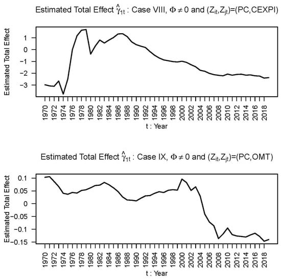
Figure 1.
Plot of the estimated total effects of CBC on RGDP in different years.
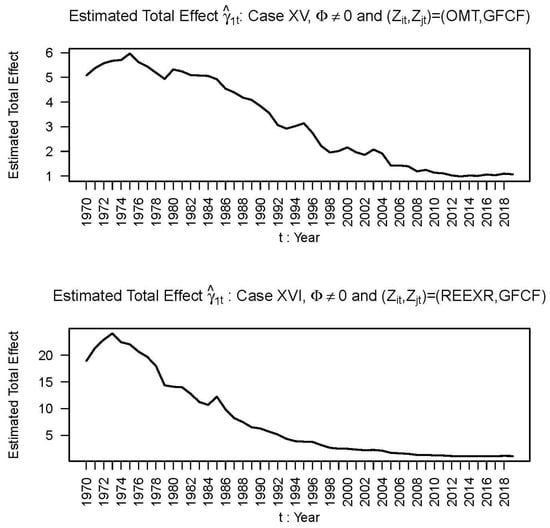
Figure 2.
Plot of the estimated total effects of CBC on RGDP in different years.
Figure 2 for Cases XV and XVI (from Table 2) shows that the estimate first increases non-monotonically in 1970, reaches a maximum around 1974, and then continues to fall non-monotonically during the period 1975–2019. For U > 0.14, there are no sizable departures from this time path of as long as the of (7) is not equal to zero and does not go below the horizontal axis. When = 0, the volatility of this time path is very high. For this reason, we should not restrict the of (7) to be equal to zero.
The most important econometric consideration we wish to emphasize in this paper is one concerning causality. To this point, underlying Equations (4)–(7) is a law which should be considered observable in light of Pratt and Schlaifer’s (1988) observability condition that in (4) be independent of in (7). This is the advantage of first addressing the simultaneity problem associated with (1) raised earlier. We may further write this law using appropriate “potential-value” notation, as advocated by Rubin (1978) and taken up by Pratt and Schlaifer (1988). Accordingly, the model in (4)–(7) coincides with its underlying law and therefore has causal implications. In this sense, the variable RGDP in (1) is caused by , whose causal effect on RGDP is the same as its total effect.
6. A Remark on the Estimators of the Fixed Coefficients of (5) and (6) without the Time-Varying Coefficients of (4)
In the statistics literature, consistent estimators are well-defined for fixed parameters but not for time-varying coefficients. Therefore, in our case, because and are not fixed, the statistical notion of consistent estimators does not apply to them. However, the coefficients of (5) and (6) are fixed, and so consistent estimators can be found for them. For these reasons, consider what happens if we remove and from (4)–(6). Combining these equations gives
where the coefficients and do not appear explicitly. Equation (9) is a fixed-coefficients model with three regressors having fixed coefficients, one interaction term with a fixed coefficient, and a heteroscedastic and serially correlated error term. One can easily develop a generalized least squares estimator based on an estimated error covariance matrix for the coefficient vector of (9). The sampling properties, including the consistency property, of this estimator are well known in the econometric literature. Even so, Equation (9) does not help us. It follows from (6) that to estimate the total effect = π10 + + u1t of of on , we need its generalized least squares estimator. The error term of (9) is + . From an estimate of this error term, we cannot get a separate estimate of . However, without a separate estimate of we cannot get a separate estimate of the sum, + + . This explains the approach outlined in Section 2 and applied in Section 3.
7. Conclusions
The total effect of commercial bank credit on real gross domestic product being the sum of certain direct and indirect effects, we have developed a new estimator for it in a model with time-varying coefficients, by exploiting a new concept: that of coefficient drivers. In applying this estimator to data for the Mauritian economy for the sample period 1970–2019, we found that the total effect is not a constant, since it increases in the initial years of the sample period and then decreases non-monotonically during the rest of the sample period in Cases XV and XVI. We report only these two cases and not other Cases in Table 2 because we consider only these two cases are reasonable.
This paper makes two contributions. The first is econometric: the introduction of coefficient drivers in the estimation of time-varying coefficients to estimate the total effects of right-hand variables on a dependent variable in a regression, thereby overcoming the ancient conundrum of how to sort out the direct and indirect effects that inevitably contaminate econometric modeling. Our method cuts the Gordian knot by achieving estimates of total effects, which, after all, is the goal of all regression estimation when randomization is not possible. In medical and other fields, where randomization is possible, researchers can follow randomization to reduce indirect effects to zero. In economics where randomization is not possible, researchers have to worry about total effects.
Our second contribution is empirical: an examination of the relationship between aggregated bank credit and RGDP in the case of Mauritius. The gradual decline of the total effects of commercial bank credit per capita on GDP per capita observed in Cases XV and XVI of Table 2 suggests that banks have increasingly played a weaker role in promoting investment that supports economic growth in Mauritius. This is a matter of concern and, therefore, further empirical work should investigate the reasons why banks in Mauritius have failed to promote productive investment during more recent times.
Author Contributions
Conceptualization, P.A.V.B.S.; methodology, P.A.V.B.S.; software, I.-L.C.; validation, P.A.V.B.S.; formal analysis, P.A.V.B.S.; investigation, P.A.V.B.S.; resources, each author’s contribution, P.A.V.B.S.; economic background and data curation, A.A.; writing—original draft preparation, P.A.V.B.S.; writing—review and editing, P.v.z.M.; visualization, P.v.z.M.; supervision, P.v.z.M.; project administration, P.v.z.M. All authors have read and agreed to the published version of the manuscript.
Funding
This research received no external funding.
Institutional Review Board Statement
Not applicable.
Informed Consent Statement
Not applicable.
Data Availability Statement
Data are available upon reasonable request to Dr Amit Achameesing.
Conflicts of Interest
The authors have no conflict of interest with any person and institution.
Notes
| 1 | For derivations and descriptions of the model considered in this paper, see Swamy (1990) and Chang et al. (1992), where it is apparent that the method of estimating total effects differs from Pratt and Schlaifer’s (1984) methodology, which we found insufficient for our purposes. |
| 2 | A new category of variable coefficient models known as state space models has emerged during the past two decades to perform time-varying coefficient estimations. However, state space models are also limited in the sense that it ignores the indirect effects of the regressor on the dependent variable. |
| 3 | It is unusual for any econometric model to have i.i.d. error term rather than an auto-correlated error term. The combination of Equations (1) and (2) has such an unusual error term. Pratt and Schlaifer (1988) employed a potential-value notation to state economic laws, each with i.i.d. error term. Equations (1) and (2) are likewise endowed with this type of error term. |
| 4 | Pratt and Schlaifer (1984, p. 13) write Equation (1) as y = + , Equation (2) as w = + e, and Equation (3) as y = ( + ) + and claim that the coefficient vector ( + ) and the error vector are unique. But, depending on the user, these vectors and matrices can differ, essentially rendering them non-unique. We maintain that this problem does not arise in our version of Equation (3). Our comment is prompted by a suggestion from William Greene that we consider issues raised by Roger Levy (2012). |
| 5 | The error term, often called a disturbance, can be thought of as the joint effect of some variables () that together with and suffice to determine the value of when the coefficients of and , including the intercept , are time-varying. While proposing the concept of omitted relevant regressors, Pratt and Schlaifer (1984) did not consider time-variability of the coefficients. |
| 6 | Full details of these estimations are available in Swamy’s Notes (Swamy 1990) on Paige’s (1979) numerically stable algorithm for the generalized least squares method. These notes also show how the method is to be applied to our model given by (4)–(7) without any rank restrictions. Additionally, Chang et al.’s (1992) paper provides a theoretical rationale for applying generalized least squares to our model with time-varying and fixed coefficients and shows how the extra information provided by the coefficient drivers (, ) is to be used. More specifically, under Assumption I, having data on , , , and Swamy’s modification of Paige’s algorithm for the generalized least squares method was used to estimate both the coefficients and the error terms of (5) and (6). From these estimates, the estimates of and of (4) are determined. The computer program we used for these computations was written by I-Lok Chang using Swamy’s mathematical formulas. To develop this program, it took us several years. We gratefully acknowledge the grants given to us by the Federal Reserve Board and the Comptroller of the Currency, both of which are located in Washington, DC. |
References
- Arcand, Jean Louis, Enrico Berkes, and Ugo Panizza. 2012. Too Much Finance? IMF Working Paper No. 12/161. Washington, DC: International Monetary Fund. [Google Scholar]
- Arcand, Jean Louis, Enrico Berkes, and Ugo Panizza. 2015. Too much finance? Journal of Economic Growth 20: 105–48. [Google Scholar] [CrossRef]
- Bagehot, Walter. 1873. Lombard Street: A Description of the Money Market. London: King. [Google Scholar]
- Berthelemy, Jean Claude, and Aristomene Varoudakis. 1996. Economic growth, Convergence clubs and the Role of Financial Development. Oxford Economic Papers 48: 300–28. [Google Scholar] [CrossRef]
- Cecchetti, Stephen, and Enisse Kharroubi. 2012. Reassessing the Impact of Finance on Growth. BIS Working Paper No. 381, Bank for International Settlements, Basel, Switzerland. Available online: https://www.bis.org/publ/work381.pdf (accessed on 5 May 2022).
- Cecchetti, Stephen, and Enisse Kharroubi. 2013. Why Does Financial Sector Growth Crowd Out Real Economic Growth? Paper presented at the Finance and the Wealth of Nations Workshop, Federal Reserve Bank of San Francisco & The Institute of New Economic Thinking, San Francisco, CA, USA, September 27; Available online: https://www.bis.org/publ/work490.pdf (accessed on 5 May 2022).
- Chang, I-Lok, Charlie Hallahan, and Swamy Aananta Venkata Bhattandha Paravastu. 1992. Efficient computation of stochastic coefficients models. In Computational Economics and Econometrics. Edited by Hans M. Amman, David A. Belsley and Louis F. Pau. Boston: Kluwer Academic Publishers, pp. 43–53. [Google Scholar]
- Deidda, Luca, and Bassam Fattouh. 2002. Non-linearity between finance and growth. Economics Letters 74: 339–45. [Google Scholar] [CrossRef] [Green Version]
- Durbin, James, and Siem Jan Koopman. 2001. Time Series Analysis by State Space Models. New York: Oxford University Press. [Google Scholar]
- Greene, William. 2012. Econometric Analysis, 7th ed. Upper Saddle River: Prentice Hall-Pearson. [Google Scholar]
- Greenwood, Jeremy, and Boyan Jovanovic. 1990. Financial development, growth and the distribution of income. Journal of Political Economy 98: 1076–107. [Google Scholar] [CrossRef] [Green Version]
- Huang, Ho-Chuan Huang, and Shu-Chin Lin. 2009. Non-linear finance and growth nexus: A threshold with instrumental variable approach. Economics of Transition and Institutional Change 17: 439–66. [Google Scholar] [CrossRef]
- Jankee, Kheswar. 2006. Banking controls, financial deepening and economic growth in Mauritius. African Review of Money Finance and Banking 2006: 75–96. [Google Scholar]
- Jouan, Karlo. 2005. Financial Liberalization in Mauritius: The Finance-Growth Nexus. Ph.D. thesis, Napier University, Edinburgh, UK. [Google Scholar]
- Kiefer, Jack Carl. 1977. Conditional Confidence Statements and Confidence Estimators. Journal of the American Statistical Association 72: 789–808. [Google Scholar]
- King, Robert Graham, and Ross Levine. 1993. Finance, entrepreneurship and growth: Theory and evidence. Journal of Monetary Economics 32: 513–42. [Google Scholar] [CrossRef]
- Law, Siong Hook, and Nirvikar Singh. 2014. Does too much finance harm economic growth? Journal of Banking and Finance 41: 36–44. [Google Scholar] [CrossRef] [Green Version]
- Levine, Ross. 2005. Finance and growth: Theory and evidence. In Handbook of Economic Growth. Edited by Steven Durlauf and Phillipe Aghion. Amsterdam: Elsevier, vol. 1A, pp. 865–934. [Google Scholar]
- Levy, Roger. 2012. Probabilistic Models in the Study of Language. Available online: https://idiom.ucsd.edu/~rlevy/pmsl_textbook/book_draft.pdf (accessed on 6 June 2022).
- Muyambiri, Brian, and Nicholas Mbaya Odhiambo. 2018. Financial development and investment dynamics in Mauritius: A trivariate Granger-causality analysis. Spoudai Journal of Economics and Business 68: 62–73. [Google Scholar]
- Nowbutsing, Baboo Mintarsingh, Ramsohok Sonalisingh, and Ramsohok Kheerty. 2010. A multivariate analysis of financial development and growth in Mauritius: New evidence. Global Journal of Human Social Science 10: 2–13. [Google Scholar]
- Pagano, Marco. 1993. Financial markets and growth: An overview. European Economic Review 37: 613–22. [Google Scholar] [CrossRef]
- Paige, Christopher. 1979. Computer solution and perturbation analysis of generalized least squares problems. Mathematics of Computation 33: 171–83. [Google Scholar] [CrossRef]
- Pratt, John Winsor, and Robert Osher Schlaifer. 1984. On the nature and discovery of structure. Journal of the American Statistical Association 79: 9–21. [Google Scholar] [CrossRef]
- Pratt, John Winsor, and Robert Osher Schlaifer. 1988. On the interpretation and observation of laws. Journal of Econometrics 39: 23–54. [Google Scholar] [CrossRef]
- Rubin, Donald Bruce. 1978. Bayesian inference for causal effects. The Annals of Statistics 6: 34–58. [Google Scholar] [CrossRef]
- Schumpeter, Joseph. 1912. Theorie der Wirtschaftlichen Entwicklung. Leipzig: Duncker and Humblot. [Google Scholar]
- Seetanah, Boopen. 2008. Financial development and economic growth: An ARDL approach for the case of the small island state of Mauritius. Applied Economic Letters 15: 809–13. [Google Scholar] [CrossRef]
- Swamy, Paravastu Aananta Venkata Bhattandha. 1971. Statistical Inference in Random Coefficient Regression Models. Berlin, Heidelberg and New York: Springer. [Google Scholar]
- Swamy, Paravastu Aananta Venkata Bhattandha. 1990. Notes on Paige’s Algorithm for the Generalized Least Squares Method. Unpublished paper. [Google Scholar]
- Swamy, Paravastu Aananta Venkata Bhattandha, and Peter Tinsley. 1980. Linear prediction and estimation methods for regression models with stationary stochastic coefficients. Journal of Econometrics 12: 103–42. [Google Scholar] [CrossRef]
- Swamy, Paravastu Ananta Venkata Bhattanatha, and Peter von zur Muehlen. 2020. Cointegration: Its fatal flaw and a proposed solution. Sustainable Futures 2: 100038. [Google Scholar] [CrossRef]
- Werner, Richard Andreas. 1992. Towards a quantity theory of disaggregated credit and international capital flows. Paper presented at the Royal Economic Society Annual Conference, New York, NY, USA, April 13–16. [Google Scholar]
- Werner, Richard Andreas. 2005. New Paradigm in Macroeconomics: Solving the Riddle of Japanese Macroeconomic Performance. London: Palgrave Macmillan. [Google Scholar]
- Werner, Richard Andreas. 2012. The Quantity Theory of Credit and Some of Its Applications. Gelang Patah: Centre for Banking, Finance and Sustainable Development, School of Management, University of Southampton. [Google Scholar]
Publisher’s Note: MDPI stays neutral with regard to jurisdictional claims in published maps and institutional affiliations. |
© 2022 by the authors. Licensee MDPI, Basel, Switzerland. This article is an open access article distributed under the terms and conditions of the Creative Commons Attribution (CC BY) license (https://creativecommons.org/licenses/by/4.0/).