Article

Modelling Seasonal Short-Run Effects in Time-Series Tourism Prices

1
Faculty of Business and Management Science, University of Novo Mesto, Na Loko 2, SI-8000 Novo Mesto, Slovenia
2
Faculty of Tourism and Hospitality Management, The University of Rijeka, Naselje Ika, Primorska 46, HR-51410 Opatija, Croatia
3
Faculty of Management, University of Primorska, Izolska Vrata 2, SI-6101 Koper, Slovenia
*
Author to whom correspondence should be addressed.
J. Risk Financial Manag. 2022, 15(5), 212; https://doi.org/10.3390/jrfm15050212
Submission received: 22 February 2022 / Revised: 20 April 2022 / Accepted: 27 April 2022 / Published: 6 May 2022
(This article belongs to the Special Issue Predictive Modeling for Economic and Financial Data)

Abstract

:
The paper’s primary purpose is to better monitor shocks; therefore, reliable scientific methods should be used to predict, monitor, and implement those events. In this paper, tourism prices are studied as an economic, I ( 2 ) and social phenomenon for better performance. The selection of inadequacies in price time series is analysed. The state-of-the-art proposed methodology step of nominal to real prices is based on monthly data using the cointegrated-vector-autoregressive model (CVAR). This is the key feature selection on time-series properties in the economy and supported software(s). An attempt at a CVAR model with five seasonally unadjusted macroeconomic variables is developed. It introduces a meaningful, genuine and indispensable new data vector of transformed variables, and this stepwise process is more appropriate against the wrong model specification. The results for the period of economic crises show that the proposed model is reliable from nominal to real prices, and the researchers implement normality to price modelling in its econometric mock-up phase. Overall, the proposed model predicts testable events for up to 48-months.

1. Introduction

Predicting tourism industry prices are essential for both inbound and outbound tourist destinations (Gričar and Bojnec 2019). Understanding the market functioning and economic behaviours; the importance of prices is critical to market economies (Couix 2021; Lemieux 2020). Therefore, the study’s objective is to develop a normal distributed econometric model for prices based on the methodology from nominal to real price modelling (Ross 2021; Chen et al. 2021). Our study is motivated to complement the applied economics methodology using publicly available secondary data (Couix 2021).
The primary objective of this research is to develop a cointegrated vector error correction (CVAR) model following Cubadda (1999), Busetti (2006), Fisher et al. (2015), Rahul et al. (2018) and Archontakis and Mosconi (2021) for better diagnosis and prediction in the financial and tourism industry. We develop and discuss time series, seasonal, I(2) and misspecification patterns for tourism inflation (Braun et al. 2013) without performing deseasonalisation to keep the data most informative (Juselius 2009).
The identified research gap has been discussed in the literature, but more often theoretically and less frequently with an applied case study. Therefore, we aim to fill the gap in the literature by demonstrating the importance of variables in aggregate values in the economy. While volatility is high in financial time series, gross domestic product (GDP) is treated as I(0), inflation as I(1) and prices as I(2).
The novelty and contribution of this study are to develop an econometric model of mixture I(1) and I(2) (Fisher et al. 2015), while I ( 2 ) differentiation is rarely presented in scientific literature and therefore worth researching. Moreover, the research aims to investigate hypotheses for short-term seasonal effects (Busetti 2006) in prices over the usual business cycles (Cubadda 1999). A step-by-step presentation shows the correctness of econometric technical processing of time series in I ( 1 ) processing, while this is mostly in general or partially omitted in applied quantitative tourism research.
Econometric methods allow analyses for price spreads and seasonal effects to vary in response to shocks (Alghalith 2007). Our procedure leads to a more robust model for misspecification, which is essential to avoid spurious results. A unique contribution is related to the two-sided effects on the economy and the possible existence of seasonal impacts on tourism prices (Claverla and Torra 2014) in the Eurozone, focusing on Slovenia as a case study using monthly statistical time series data.
The data vector is split into the testable period. The division of the time vector follows the Organisation for Economic Cooperation and Development (OECD 2013), which states that green tourism has to be started and will last for many years. Therefore, the data vector (2000–2017) considers tourism prices as critical growth factors. During these periods, potential shocks can be related to specific events and developments such as Slovenia joining the European Union (EU) and adopting the euro, experiencing high food prices, witnessing economic crises, and economic growth. The focus is on the hospitality sector within the tourism industry, which makes up the most significant part of the tourism industry in Slovenia.
The paper’s primary goal is to present volatilities in economics time series data to show how they can be treated in econometrics beyond misspecification tests. The rest of the paper is divided into four sections: literature review, the methods and data used, presentation of the results, and discussion.

2. Literature Review

In Dash and Parida’s (2013) and Kumar and Patel’s (2021) studies, cointegration was used to model tourism demand and forecasting. The evidence was linked to unit root tests and structural breaks (Capelli et al. 2021; Lin and Huang 2012). In addition, Kunst and Frances (2015) investigated seasonal time shifts in weekly time series.
Some studies (Claverla and Torra 2014) have identified continuity cycles; there have been few research efforts aimed at analysing time series data (Qi et al. 2012) in a dynamic regression model using a vector autoregressive model (VAR) (Kulendran and Witt 2001). The stability of responses to price changes can be affected by different determinants in people’s expectations and the national economic situation (Smeral 2012).
Time-varying volatility is in the direction of a dynamic regression model (Harvey 1989; Song et al. 2009), as the model VAR (Juselius 2015; Koukouritakis et al. 2015). This can imply stubbornness in the specification of the tourism model and allow for structural instability (Harvey 1989; Song et al. 2009; Koukouritakis et al. 2015). The time-varying parameters approach (Braun et al. 2013) gives more weight to the most recent data evaluating tourism demand and price models and leads to more accurate projections than the commonly used regression models (Kulendran and Witt 2001). This step is essential to capture structural changes or unanticipated shocks (Juselius 2015) in econometric models of tourism (Song et al. 2009; Claverla and Torra 2014; Kumar and Patel 2021).
The time-varying parameter approach (Qi et al. 2012) is functional when dealing with structural changes (unexpected shocks) (Kulendran and Witt 2001; Koukouritakis et al. 2015) but does not provide robust results when testing the assumption that the value of the elasticity varies depending on the phase of a particular business cycle (Smeral 2012) of the economy or unexpected shock (Juselius 2015; Kumar and Patel 2021). This is crucial for predicting conditions (Claverla and Torra 2014) typical of an economic downturn or stagnation, with different price consequences at various stages of prosperity (Smeral 2012). Moreover, using the recursive ordinary least squares (OLS) method shows that the assumption of coefficient constancy is too restrictive (Song et al. 2009) and that macroeconomic variables are highly dependent (Juselius 2015).
This paper critically examines the approach of simple static regression analysis, a commonly used statistical technique (Johansen 2012; Juselius 2015), and highlights the validity of the underlying assumption of simple static regression analysis to draw attention to some shortcomings where this method cannot be routinely used. This is the case when variables are non-stationary (Kulendran and Witt 2001), either because they exhibit a deterministic trend (Papell and Prodan 2014) or, more commonly in macro econometrics, a stochastic trend (Juselius 2015; Huang et al. 2015).
A demonstration of the econometric model is evidenced by the econometric composition agreeing and suggesting the non-stationary variables (Johansen 2012) when implementing the CVAR model, which can better express the understanding of the variation of the time series vector (De Mello and Nell 2005). CVAR application can be highly relevant to a better understanding of time series data. The concern about the misuse of correlation coefficients between economic variables is also applicable in determining variables. The CVAR thwarts the problem of trend adjustment by specifying the general VAR in terms of an error correction that includes all deterministic components: Trend, Constant, and Dummy Variables (Juselius 2015; Dash and Parida 2013). In a dynamic regression model such as the VAR, a dummy variable controls for the unexpected shock but leaves the measurement unaffected. This contrasts with a regression model where a dummy variable usually eliminates the measure of the irregularities in time-series development (Kulendran and Witt 2001; Juselius 2009).
Emerging and developing economies have mostly undergone a transition and have suffered from an inflation treatment that exceeded the main constant several times. Therefore, inflation was maximised by policy changes and minimised by external influences, such as the emergence of integration content. A subdued inflation rate was usually seen as costly in output losses and adjustments of tourism prices to seasonal changes. However, a better understanding of the role of assumptions has given policymakers hope that credible monetary and industrial policies can achieve disinflation without negatively affecting actual economic activity in tourism (Baxa et al. 2015). The findings reveal deficiencies in research on macroeconomic variables in tourism and economics on the appropriateness of time series.

3. Materials and Methods

As a starting point is an illustrative example of two time-series X t and Y t , t = 1 , , T , and a substantive theory (Kulendran and Witt 2001):
Y = β · X ,
that X influences Y in a linear fashion formulation.
The data obtained may not be in the same relation, and there is usually no theory behind them. Haavelmo (1943) argued that we need some deterministic proposal and problem to solve this stochastic property in odds, which should be as elastic as possible (Juselius 2022), which has been further developed by Johansen (2012).
We introduce:
Y t = β · X t + ε t ,     t = 1 , , T ,
with the error term ε t in a statistical relation (Juselius 2009).
When the model deals with the hypothesis about the parameter β that β = 0 , linear regression and correlation analysis are essential. In this sense, the independent variables affect the dependent variable in a time frame on some lag, but the independent variables do not affect each other. First, the regression approach is used to estimate the effect of X on Y using the following expressions (Johansen 2012):
β ´ = t = 1 T X t · Y t t = 1 T X t 2 ,   and
σ ´ = T 1 · t = 1 T ( Y t β ´ · X t ) 2 ,
by calculating the least-squares estimators and the residual error variance. These interpretations are then used to perform boundary behaviour inference by analysing the t-ratio:
t β β 0 = ( t = 1 T X t 2 ) 1 / 2 · β ´ β 0 σ ´ ,
with the quintiles of a standard normal distribution. The regression approach straggles well if the estimators β ´ and σ ´ 2 are halt to their analytical observes, β and σ 2 and if the boundary behaviour distribution t β β 0 is close to the Gaussian distribution (Johansen 2012).
Second, a widely known problem of normally distributed residuals ε t is i.i.d. N ( 0 , σ 2 ) in regression analysis that does not link empirical regression to theoretical values. There is also the issue of stationarity and X t is nonstochastic (Qi et al. 2012). Similarly, if ( X t ,   Y t ), then is i.i.d. Gaussian with variances σ 1 2 ,   σ 2 2 , and covariance σ 12 . The theoretical correlation is then ρ = σ 12 / σ 1 · σ 2 , and the maximum likelihood estimator of ρ is ρ ´ . In addition to saying it has a publicly refreshed idea not to check the model and compare the econometric model as it fits the data, it just seems to click on the computer as a very convenient task (Johansen 2012). Testing the model with multiple indicators and plots gives the researcher a model-based and suitable econometric approach, i.e., providing accurate results (Kulendran and Witt 2001; Juselius 2015).
To further discuss the vulnerability of the econometric conclusions, the modelling process is the subject of this research, while the evaluation of the systems with applied economic results is of great importance, which increases after each negative shock. The methods used in the applied part of the research are regression analysis, VAR CVAR models and Granger Causality.

3.1. Regression Model

The regression model in its statistical version is performed as written in Equation (2) where   ε 1 , ,   ε T permutations in the commitment that they are, i.i.d. (0, σ 2 ) and ε t is independent of X 1 , ,   X t ,   t = 1 , , T ;   X 1 , ,   X t are variables in their stochastic or deterministic dispersion and statistical inference conforms to linear constraints (Johansen 2012):
n T 1 t = 1 T X t 2 P > 0 ,
for some sequence n T .
Here P stands for convergence in expectation (Hall and Heyde 1980). Johansen (2012) shows four results when the regression method works well.
The following approach is used when the regression approach may fail using the time series data. When it cannot be normalised
t = 1 T X t 2 ,
in a way that the limit exists as a deterministic limit, it can be called a random walk regressor. In the case that ξ = 1 , then there is a unit root, so that X t is stochastic and non-stationary (Kulendran and Witt 2001; Huang et al. 2015) in the sense that (Johansen 2012)
X t = i = 1 t ε 2 i + X 0 ,
and in this case, E ( X t X 0 ) = X 0 and the variance V a r ( X t X 0 ) = σ 2 2 · t , which increases to infinity. However,
T 2 i = 1 T X t 2 ,
sets a stochastic variable and does not converge to the deterministic term. The detailed theory involves Brownian motion (Johansen 2012), an uninterrupted stochastic operation defined on the unit interval 0 u 1 by random walks. Two fundamental results of the Brownian motion are stochastic variables. Convergence in modelling is normalised for this study to product moments, which should be T 2 and T , respectively. The significance is that the stochastic implication is imposed (9), while it is based on the conditional process. The regression coefficient satisfies:
β ´ P μ 1 μ 2 ,
this is the ratio of the slopes of the trends. An applied analysis of the time-series data, using models:
Δ Y t = ε 1 t + μ 1 ,
and
Δ X t = ε 2 t + μ 2 ,
is to make linear assumptions for each contained variable and estimates of μ 1 and μ 2 to talk freely about the information contained.
It is of utmost importance that the variables in the time series approach are entirely uncorrelated, as they are not variables in levels, which is why a regression approach is invalid, while in the case of correlated variables, they are distinguished by a third term, which most likely corresponds to a time trend (Juselius 2009, 2022). It is critical to note that in the calculus of correlations to replace E ( X t ) and E ( Y t ) by acceptable estimates we should not use the time series data averages.

3.2. The Cointegration and VAR Model

The random walk (De Mello and Nell 2005) and co-relations (Granger 1981) in macroeconomic variables are higher-order problems; hence, cointegration was introduced (Juselius 2022). Engle and Granger (1987) tested cointegration by applying regression models. Phillips (1991) and Johansen (1988) identified the valid interpretation of the regression model and noted the autocorrelation problem within the cointegration exercise. The technique of cointegration has become a research approach in time series econometrics and statistical computer program packages, such as CATS for RATS (Dennis et al. 2005).
We consider two variables X t and Y t , which are generated by the equations (Johansen 2012):
Δ Y t = τ · ( Y t 1 γ · X t 1 ) + ε 1 t ,
Δ X t = η · ( Y t 1 γ · X t 1 ) + ε 2 t ,
for t = 1 , , T . The linearity in each variable is progressive. The time series contains information from the past, but it should be noted that the levels of the variables Y t 1 and X t 1 all occur in the same order
U t 1 = Y t 1 γ · X t 1 ,
in each of the comparisons. The U t 1 is the disequilibrium error and the consumption Y = γ · X as a mean relation. Thus, the variables respond with adjustment coefficients τ and η , respectively.
Such a model contains a stationary variable part and a random walk, generating non-stationary variables. Interestingly, the combination in a linear sequence is stationary so that the linear combos ( 1 , γ ) eliminate the common trend (random walk). Thus ( X t , Y t ) is non-stationary but has a property of a collected time series variables and has a cointegrating vector ( 1 , γ ) and routine stochastic trend S t (Granger 1981).
It is worth noting that unlike a regression of Y t as a function of X t , the variables are treated and modelled similarly. Thus, for example, if Y t γ X t is stationary; after that, the result is γ 1 Y t X t . The normalisation procedure could therefore be provided on non-zero coefficients on both variables.
In cointegration, there is no causality processing, underlined by the VAR model with two lags and constant within the n —dimensional process and X t is developed by the equation:
H r :   Δ X t = α · β · X t 1 + Γ · Δ X t 1 + μ + ε t ,
where the white noise process ε t = x t μ t is the difference between the stipulatory mean μ t and true comprehension X t , which usually is independent N I n ( 0 , Ω ) , t = 1 , T , and ( α ,   β ) are n × r matrices, r is cointegration rank, X t 1 are past values of the variable, Δ X t is differenced variable, μ is a mean vector for all periods T , and Γ is a covariance matrix (Johansen 2012). The technical process of I ( 1 ) has the relevance of avoiding obstacles in distinguishing error specifications, such as the i.i.d. assumption of error terms and plot analysis. Most importantly, the lag lengths should be examined to check the time series assumption behind the model and finally to identify the cointegration rank for estimating the model under the development interpretation. In conclusion, the beta-normalised constraints on zero are essential (Johansen 2012; Juselius 2022).
It is essential to check the rank of α and β in time series to obtain the number of cointegrations. The starting point is the unrestricted model VAR:
H n :   Δ X t = Π · X t 1 + Γ · Δ X t 1 + μ + ε t ,
where ε t i.i.d. N ( 0 , Ω ) and Π ,   Γ ,   μ , and Ω are unrestrained. The cointegrating relation is assumed over r and is formulated as in the VAR model with two lags and a constant term:
Π = α · β ,
where α and β are n × r matrices ( n < r ) and the r combinations β · X t , which define the stationary relation of non-stationary variables (Juselius 2015). In conjunction with maximum likelihood estimators, estimators can be computed definitively by an eigenvalue problem, even if it is a non-linear maximisation snag for a separate rank regression or for introducing cointegration (Johansen 1988). The latest provides estimators ( α ˇ , β ˇ , Γ ˇ , μ ˇ , Ω ˇ ), calculated from:
T 2 [ l o g d e t ( Ω ) · 1 2 t r { Ω 1 · t 1 T ε t ( Π ,   Γ ,   μ ) · ε t ( Π ,   Γ ,   μ ) } ] ,
and the highest point L m a x   ( H r ) . At this point, the input is a misspecification test. The model’s boundary is perceived by a unit root test developed by the so-called Dickey-Fuller -test (Dickey and Fuller 1981) for the uni-modelled process and the misspecification test for the multivariate VAR model depending on one or more deterministic terms. Overall, modelling procedures include not only the chi-squared test but also the likelihood ratio test or the t −test statistic, where χ 2 ( f ) in an f recognises the number of restrictions used in a parameterisation procedure (Johansen 2012; Juselius 2015, 2022).

3.3. The CVAR Model

Shocks are a common problem in economics. Volatility in series called shocks or breaks provide several valuable pieces of information for researchers. Such a violation pushes the variables out of the mean or equilibrium. In comparison, high correlation matrix coefficients affect the predictability and usefulness of time series modelling and reveal biased results. Therefore, ordinary stochastic trends are required in bivariate cointegration, but only more than two variables are usually needed to produce cointegration. Illustrational cointegration is more related to multiple regression, with one significant difference. The cointegration results are sensitive to the length of the data vector, while the regressors in regression are sensitive only to orthogonality. The importance of such thinking in an economic modelling process creates non-multicollinearity, while cointegration is realised in the set of variables. (Kulendran and Witt 2001; Juselius 2015). We present the CVAR model (De Mello and Nell 2005) applied to analyse the tourism time-series (Kunst and Frances 2015) data considering the non-stationarity. The CVAR model circumvents the problem of misuse of correlation coefficients between economic variables by inventing the VAR in the error-correction model (Juselius 2009; Kulendran and Witt 2001):
Δ X t = μ 0 + Π · X t 1 + Γ · Δ X t 1 + Γ k 1 · Δ X t k + 1 + Φ · D t + ε t ,     t = 1 , T , ε t ~ N I D ( 0 , ) ,
where Φ · D t includes each deterministic component (trend, constant, and dummies). The hypothesis that X t is integrated of order one ( X t   ~   I ( 1 ) ) is invented as a reduced rank condition (18). For simplicity, only two lags are included in (Johansen 2012) the CVAR model, which leads to:
Δ X t = μ 0 + α · β · X t 1 + Γ 1 · Δ X t 1 + Φ · D t + ε t ,     t = 1 , T , ε t ~ N I D ( 0 , )
by converting the trending variables, X t , into stationary differences, Δ X t , and stationary cointegration relations, β · X t , the multicollinearity is solved. One can find stationarity between the components of the regression and correlation coefficients, which are now well defined for given β , and standard inference ( α ,   Γ 1 ,   ) holds. The model is non-linear in α and β , but can be evaluated by the reduced rank proposed by Johansen (1988) where the β factors are treated as the eigenvectors to a mix of an eigenvalue problem, and α is calculated by linear regression for given β . The definitions β · X t define r linear relationships between n variables.

4. Results

We use five seasonally unadjusted monthly time series price variables. The in-sample is from January 2000 to May 2012, and the out-of-sample is from June 2012 to December 2017. The specified variables are: Slovenian prices in the hospitality industry ( I P H I t ), prices in the hospitality industry in the Eurozone ( I P H I E A t ), Slovenian consumer prices ( C P I t ), consumer prices in the Eurozone ( C P I E A t ), and Slovenian food and beverages prices ( I F B t ) as input costs for the hospitality industry. The initial VAR methodology is used, and the price differences are involved in the approach.
The data are obtained from the Statistical Office of the Republic of Slovenia (SORS 2021) and Eurostat (2021).

4.1. Inflation and Tourism Prices

4.1.1. Regression Analysis

Following the introduced simple static regression model in Equation (2), we would like to find effects on the I P H I t . Hence, I P H I E A t ,   C P I t ,   C P I E A t , and I F B t are the most likely determinants influencing the I P H I t . Calculating the static regression model in Equation (2) with the used explanatory variables, we get the following regression results:
I P H I t = 1.527 ( 6.270 ) · I P H I E A t 0.139 ( 1.470 ) · C P I t + 0.832 ( 3.292 ) · C P I E A t + 0.335 ( 5.857 ) · I F B t + S D ,
where SD denotes seasonal dummy variables. From the t -test numbers in the brackets can be seen the statistical significance of the regression parameters. A final step is to transform variables with seasonal adjusting. We get:
I P H I t = 2.478 ( 7.246 ) · I P H I E A t 0.277 ( 2.852 ) · C P I t + 0.045 ( 0.140 ) · C P I E A t + 0.288 ( 5.186 ) · I F B t 0.053 ( 0.400 ) · t ,
where the time variable t runs from 1 to 129. High statistical significance is observed by almost regression parameters of all variables, except for C P I E A t . The Durbin-Watson statistic is lower than 2 (0.813), indicating the presence of autocorrelation (Kulendran and Witt 2001). The adjusted determination coefficient is high at 0.992, and F statistic is significant by 3005.9.
The partial autocorrelation graphs confirmed the first and twelve lags, and the autocorrelation are at least in the first order. The residuals are not i.i.d. Results show spurious regression (Kulendran and Witt 2001) and cannot be normalised as a deterministic limit as explained in Equation (7). There is a unit root, and X t is stochastic and non-stationary theoretically expressed as explained in Equation (8).
Time series for inflation can be considered stationary or non-stationary (Baxa et al. 2015). This statement is due to a unit root process (stochastic trend), and inflation should instead be treated as a non-stationary variable. It is crucial to start with a shorter duration, 3 to 5 years, which leads to a non-stationary formulation, and the cyclical component can be further studied in a more extended period, e.g., 13 years, for the example of this approach. Nevertheless, this is tested in the forecasting OLS in Appendix H.
The distinction between short- and long-term cycles is that a long/short term cycle can be treated as either non-stationary or stationary, depending on the time perspective of the work (Juselius 2022; Gričar and Bojnec 2021).
Juselius (2009) shows that prices enter a two-sided inverse stochastic trend that can be written as P t ~ I ( 2 ) when the inflation rate is integrated with a non-zero mean. The order of integration is known as the number of times a series should be differentiated to achieve stationarity (Kulendran and Witt 2001). Most research treats variables in levels or seasonally adjusted terms and rarely examines parameters involving real variables and their transformations. This contributes to the fact that prices are standardised in the almost second order of integration (Gričar and Bojnec 2019). I P H I t ,   I P H I E A t ,     C P I t ,   C P I E A t , and I F B t should be preceded by the I ( 1 ) analysis of the real price variables (Juselius 2009).

4.1.2. The Data Vector

An additional formulation is obtained by taking logarithms, where now new names of variables indicate a logarithmic transformation and a symbol R indicates that the variable was transformed from nominal to real, r indicates real t time series variable, and variables are at least I ( 1 ) ; X t r ~   I ( 1 ) . Therefore, we decided to use the logarithms transformed C P I E A t   and I P H I E A t . We have transformed variables from nominal to real prices using i.i.d. process checking to become stationary in I ( 1 ) .
Data on time-series prices are at most X t ~ I ( 1 ) (Juselius 2009). We get the data vector: [ r p h   r p   r f b p   d p e a   d p h e a ] t T , t = 2000 : 1 , ,   2012 : 5 , whereas the minuscule letters define normally distributed residuals, e.g., real or differenced variables. The transformation procedure is in Appendix A.
To clarify precisely whether the variables are endogenous or exogenous, it is essential to look at them from a stochastic point of view. They are tested for long-run cointegration as explained in Equations (13) and (14) using OxMetrics (CATS for RATS) software (Tufte 1998). In the short run, seasonal effects were calculated in a dynamic error correction model explained in Equations (20) and (21) using OxMetrics software.

4.1.3. Misspecification Test

The formal misspecification tests (Appendix A, Table A1) have confirmed that the VAR model neither contains autocorrelations nor heteroskedasticity in the residuals. We also assume the test of normality formed on skewness and kurtosis of the standardised estimated errors. The null hypothesis of the normality test is not rejected (p = 0.356). Checking the stability of the VAR model, this derives to the conclusion that there are several permanent dummies needed for analysing structural breaks and/or shocks (Çağli and Mandaci 2013; Lin and Huang 2012), where the most obvious one, by using the visual inspection of the VAR model, was a shift dummy for high decreasing prices in the hospitality industry in September 2010 ( D s 109 t ). This dummy is foremost valid to normalise the cointegration equations. Other permanent dummies as a one-time effect (Kulendran and Witt 2001) are: the 11 September attack (September 2001), the euro having been circulated in its physical form (January 2002), decreasing the hospitality industry prices in the Eurozone (October 2004), a month before Slovenia adopted the euro (December 2006), and the period of high food prices (September and November 2007):
Δ X t = Γ 1 · Δ X t 1 + α · β · X t 1 + ϕ p .1 · D p 019 t + ϕ p .2 · D p 021 t + ϕ p .3 · D p 0410 t + + ϕ p .4 · D p 079 t + ϕ p .5 · D p 0711 t + ϕ p .6 · D p 0612 t + ϕ s .7 · D s 109 t + γ 0 + ε t ,
are involved in the CVAR model in Equation (21) but not in the cointegration relations in Equations (25) and (26). The residuals from the estimated VAR (2) model with dummies now contains improved properties compared to the unconstrained model, as explained in Equation (16).

4.2. Specifying the VAR Model and Empirical Results

4.2.1. Test of Cointegration Rank, Long-Run Exclusion, and Stationarity

There are no trends in the variables’ levels, but non-zero means exist in the cointegration relations. We restrict the CVAR model that the rank of Π is r , meaning that the five variables in the model have r cointegration relations and n r common stochastic trends. We estimated the CVAR model for r = 1 ,   2 ,   3 ,   4 ,   5 . We consider the LR (Johansen 1988) trace test of cointegration rank. We have found the rank of two: r = 3 (Table 1), where p -value is 0.003. Moreover, r = 2 is at p -value 0.000, and r = 4 is at p -value of the trace test 0.440.
We consider how to formulate tests of various hypotheses on the cointegration vectors. In the first step, we consider the test for the long-run exclusion of a variable, i.e., a variable that can be removed from the cointegration space. We have estimated the model with a D s 109 t and manually included the first difference with one lag, and we imposed a rank of r = 3 . We will consider the Π matrix (Table 2).
The variable is excluded from the cointegration relations when the coefficients in the respective column of the Π matrix are insignificant. From the Π matrix in Table 2, there are no clear signs that any of the variables can be excluded from the cointegration relations, except for the r p h t (Table 2). The design matrix Π for the hypothesis that the first variable can be excluded from the cointegration relations is where s is the number of free parameters. We restrict one of the n = 7 variables (5 variables, shift, and a constant), and we have six free parameters.
The test of long-run exclusion (Table 3) can be performed automatically in CATS for RATS for different choices of rank. For a rank of r = 3 , none of the five variables or the restricted level shift can be excluded from the cointegration relations, except for the r p h t . However, we have decided that the r p h t the variable will stay in the model specification because we would like to test long-term and short-term relations on this variable in a cointegration space. Moreover, if we choose a cointegration rank of r = 1 , then we can exclude the r p h t , and d p e a t 1 . Furthermore, the constant can be excluded so that the single cointegration relation in the model is a relation between the inflation rates and the food and beverage prices.
If variable i is stationary around a constant mean value with a D s 109 t , then one of the cointegration relations must be given by a linear combination of variable i , the constant term and the level shift. When testing for stationarity of variable i we restrict one of the cointegration relations to variable i , the constant term and the level shift, while we leave the other cointegration relations unrestricted. For r = 3 we restrict one relation while keeping the other unrestricted. For a rank of r = 3 , the tests given from CATS for RATS are equal to the manually calculated tests. For r = 2 (and r = 1 ), none of the variables are stationary by themselves.
Note that the choice of the cointegration rank matters for the stationarity of the single variables. For r = 3 the d p e a t 1 and the d p h e a t 1 , they become borderline stationery, which means that a linear combination of them can give the third cointegration relation d p e a t 1 and the d p h e a t 1 with the constant term and the level shift. The significance level is: 0.333 for the d p e a t 1 and 0.288 for the d p h e a t 1 , when r = 2 . The result can be seen in the second raw in Table 3.

4.2.2. Test of Weak Exogeneity

We want to impose a test of a long-run weak exogeneity, as presented in the third row in Table 3. A variable is weakly exogenous for the long-run parameters if the variable is not adjusting to the long-run equilibrium error given by the cointegration relations. A weak exogeneity means that the variable has a zero-row in alpha so that the variable does not react to beta. A zero-row in alpha corresponds to a unit vector in alpha orthogonal. Alpha orthogonal defines the ordinary stochastic trends in the model. The weakly exogenous variable determines the endogenous one by pushing the effects out of equilibrium, and therefore the ordinary stochastic trend is involved in one variable in the opposite direction.
We look at the evidence of a weak exogeneity in Table 3. We can note that all variables react to almost all the other variables. We can thus accept the joint hypothesis of the non-weakly exogenous test. All variables have a p-value of at least 0.020 already when r = 2 .

4.2.3. Long-Run Cointegration Relations and Restrictions on β

The restrictions based on the previous theoretical scenario are imposed. The nineteen over-identifying restrictions held stationarity and were tested using the likelihood ratio (LR) test procedure parameterised in Johansen and Juselius (1994). The restrictions were accepted with a p-value of 0.732. The restrictions are formulated in an econometric approach with a path where all β coefficients are statistically and empirically correct.
The first long run cointegration vector ( C I a ) is:
d p e a t 1 = 0.004 · r p h t + 0.397 · d p h e a t 1 0.002 + ϵ t ,
and is normalised by restrictions on β on the real consumer prices in the Eurozone. They are negatively related to the real Slovenian hospitality industry prices, representing a small but statistically significant effect of the national sector economy on the expected inflation in the Eurozone, and positively related to the real prices in the hospitality industry in the Eurozone, respectively. The constant term shows that consumer prices in the Eurozone declined.
The second long run cointegration vector ( C I c ) is:
d p h e a t 1 = 0.005 · r f b p t + 0.866 · d p e a t 1 0.001 · D s 109 t + ϵ t ,
and is a function of the hospitality industry prices in the Eurozone. The real prices in the hospitality industry in the Eurozone are positively related to the real Slovenian food and beverages prices and real consumer prices in the Eurozone, respectively. The shift dummy is in harmony with a small decrease in real prices in the hospitality industry in the Eurozone following the economic crisis. A confirmation of the stationarity of the shift dummy is imposed, and the result is consistent with some recent findings (Juselius 2022; Gričar and Bojnec 2019).

4.2.4. The Cointegrated VAR Model in the Short Run: Empirical Results

In a dynamic equilibrium error correction or CVAR model (Juselius 2009), the non-significant lagged variables are removed from the system based on the calculated and confirmed cointegration relationships. This procedure is determined using the F-test, with insignificant coefficients extracted using the LR test.
Except for a negative correlation between the d p e a t 1 and r f b p t (−0.41) shocks, the remaining cross-correlations are essentially more or less zero. The column headline in the top half of Table 4 denotes the dependent variable. The row headings indicate the shape variables. The estimated coefficients of the included dummy variables are also reported in Table 4.
Table 4 can be seen as a statistically significant impact on d p h e a t 1 in the short term. First, impacts on d p h e a t 1 are long-term cointegration vectors C I a and C I c . Secondly, we also find an enormously significant relationship between the season’s dummies and d p h e a t 1 . Several permanent dummies are also significant such as January 2002, October 2004, and September 2009. We can conclude that prices in the hospitality industry in the Eurozone declined in almost all circumstances. The decline is by seasonal effects, cointegration relations, and consumer prices in the Eurozone. They increase only before and after the high season, e.g., June and September.
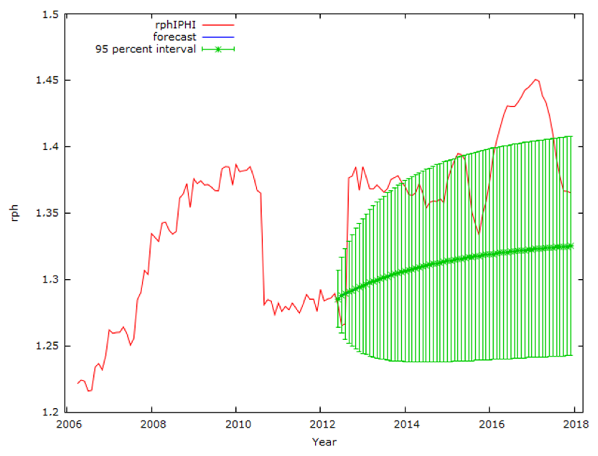
The empirical results validate the existence of a valid long-run cointegration relationship with short-run parameter constancy. The direct implication of our results is that the short-run model is robust only if the long-run cointegration parameters are included in the model. These findings are vital to a short-run model specification, including different assumptions about whether time-series variable(s) is/are contemporaneously exogenous. The inclusion of the Eurozone and Slovenian hospitality industry prices in the analysis is the correct specification given the tremendous impact of seasonal short-run effects on tourism prices, and therefore, forecasting them as presented in Appendix E.
Our empirical findings on the short-run effects on tourism prices have additional noteworthy implications for empirical economics and modelling in tourism, adopting new modelling shreds of evidence. The differences in the implementation of tourism modelling in our study shed some light on how the performance of correct variables and statistical models affect the short-run effects. The main benefits of short-run model results of tourism prices include: first, moderation of the level and volatility of prices and inflation; second, analysing the structural breaks in business cycles; and third, following the misspecification test are exclusion test, rank test and test of restrictions on β .
This time-series data research could be extended to more countries using the euro as a national currency. Such extended time-series data research would represent the studied determined impact of a specific country on the hospitality industry prices in the Eurozone and consumer prices in the Eurozone. From the methodological point of view, the research can be extended to Granger causality between the variables as presented in Table A2, Appendix G.

5. Discussion

We have critically evaluated the simple static regression analysis approach in the literature, which is often used to analyse time-series data. We have also presented non-stationarity with unit roots and stochastic trends/shocks. Instead of simple static regression analysis, we apply the CVAR model to analyse time-series data for tourism prices. This is a novelty and a contribution to the theoretical literature.
We first tested the time-series properties of each variable and restrictions in the VAR model. The nominal time series prices are integrated with order two, and the VAR model includes a linear transformation of the tourism prices and inflation variables. We reformulated the VAR model with the transformed variables without losing information when the restrictions were imposed. Therefore, we decided to use variables of order one.
The formal misspecification tests confirmed that the VAR model does not contain autocorrelations or heteroskedasticity in the residuals. Normality tests based on skewness and kurtosis are used to check the integrity of the standard residuals of the model and variables. Normality tests based on skewness and kurtosis are used to check the integrity of the standard residuals of the model and the variables. As part of this process, the stability of the VAR model was developed, and the propositional condition of the different dummies should be included.
The unrestricted VAR model has two lags and a rank of three; the eigenvalues are derived using the trace or Johansen test. In the restricted VAR model, there are non-weak exogenous variables. In this sense, all five time series data are endogenous variables. We apply a test for the short-run cointegrated VAR (CVAR) model. We can find that prices in the hospitality sector in the euro area have fallen in almost all circumstances. The decrease is due to seasonal effects, except in June and September when they increase due to long-run cointegration relationships and consumer prices in the Eurozone.
The long-run cointegration relationship normalised to β-coefficients for the hospitality prices in Slovenia was not found. Moreover, the test of long-run exclusion and the results of the combined effects of the Π-matrix suggest that the Slovenian hospitality prices should be removed from the CVAR model. This conclusion confirms the research objectives for the economic modelling literature: simple regression analyses cannot be performed for dynamic time series models where the Slovenian hospitality prices are a significant dependent variable. We point out that a long-run cointegration relationship in modelling short-run effects of “nominal to real” prices is necessary as robust evidence for analysing tourism price trends.

6. Conclusions

This study defined a state-of-the-art empirical model on general and sectoral prices in Slovenia and the Eurozone. The main objective was to build a theoretical model and test the robustness of the econometric model. Since prices explore high volatility, the primary purpose was to investigate volatility and perform an objective CVAR modelling procedure as a technical step for reliable modelling and prediction.
The importance of inflation in the econometric procedures was primarily discussed by Juselius (2009); therefore, this research fills the gap in the literature by showing the time series conformances. The volatility of prices was identified and confirmed. The normalities on the residuals were challenging to obtain and led to several findings:
  • essential step: the nominal to a real transformation of the variables;
  • the definition of the econometric model: several deterministic coefficients needed;
  • a guarantee of the corresponding cointegration rank with a slight lag difference;
  • and defining cointegration vectors and relations of the short-run effects on tourism prices.
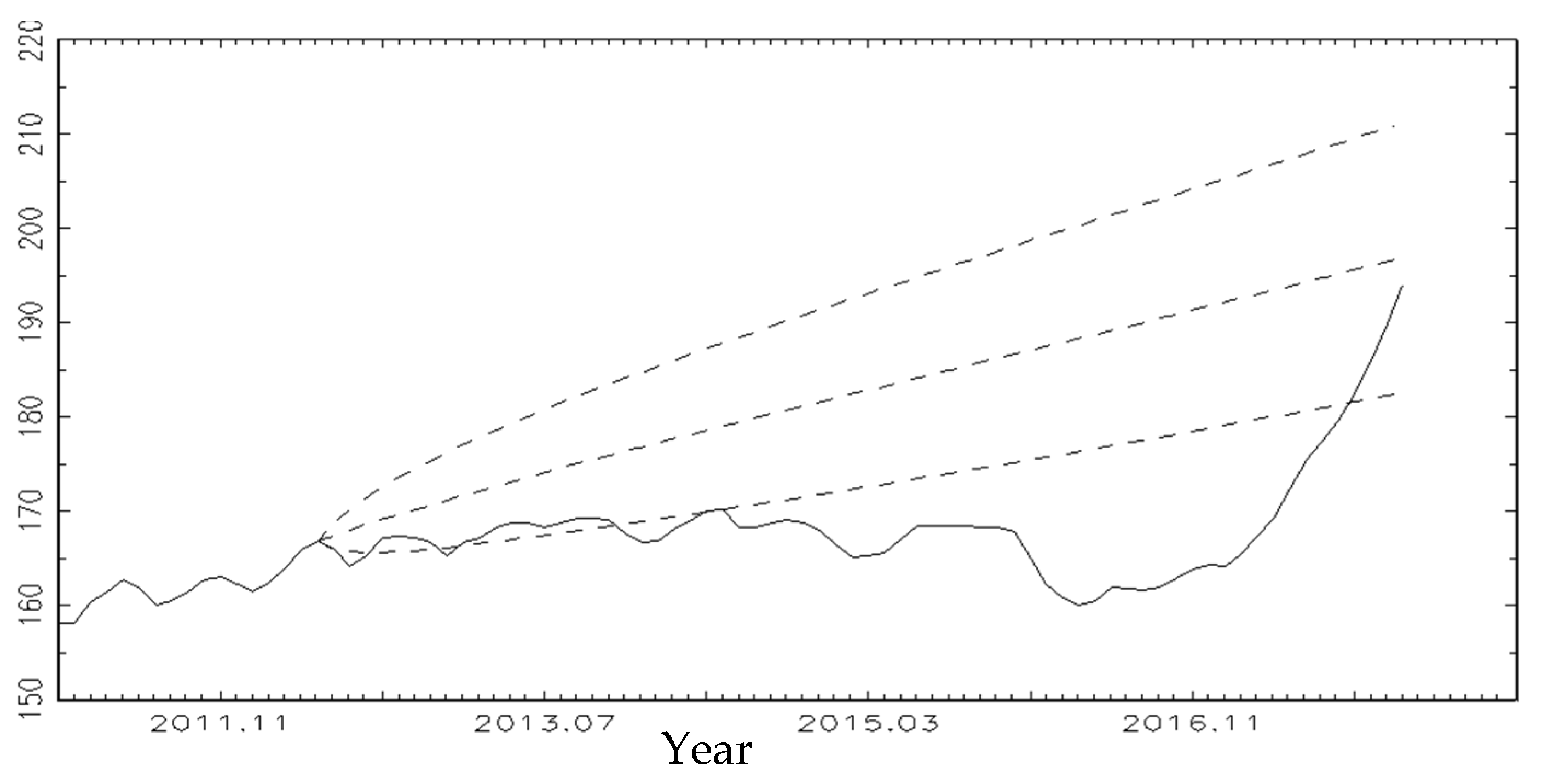
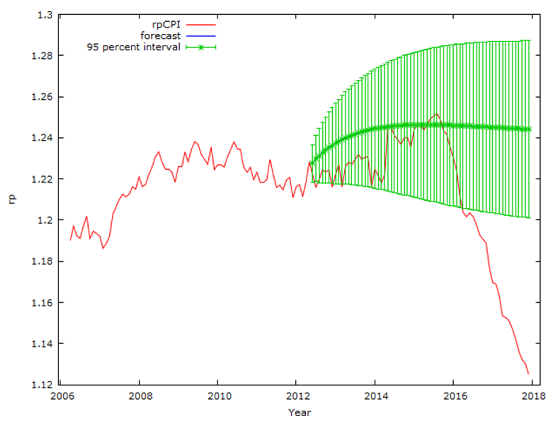
The theoretical importance of the study is reflected in the technical procedure that must be carried out before applying the model to an empirical sample. The empirical implication is defined in a reliable empirical model based on econometric steps that can subsequently predict the future dispersion of the data, which is presented in Appendix B, Appendix C, Appendix D and Appendix F. The outlook on these results shows that the model has high conformance for the first 48 months, while only a few outliers were detected. Nonetheless, in the last period of the sample, some more substantial downward fluctuations in consumer price indexes and the food and beverage index were observed. This striking result could also explain the increase in prices in the following periods up to the present.
Overall, the study has some limitations as possible issues for research in the future:
  • the data have not been deseasonalized. This decision is based on extracting as much as possible from the raw data;
  • the sample period is limited to the most severe period of the 2008 economic crisis.
In summary, this study has added an essential scientific and technical step to the definition of econometric modelling of time series using aggregate values, leading to a big data adventure in future phases. However, in the appendices, one can find the benchmark models for predictive modelling of cointegrated behaviour of time series in tourism, which has been primarily omitted in tourism research. Therefore, this research adds value to management policy analysis for decision-making and economic theory at the integration level to obtain the most appropriate and meaningful forecasts and models for tourism pricing.

Author Contributions

Conceptualisation, S.G. and S.B.; methodology, S.G.; software, S.G.; validation, S.G., and S.B.; formal analysis, S.G.; investigation, S.G.; resources, S.G.; data curation, S.G.; writing—original draft preparation, S.G.; writing—review and editing, S.G. and S.B.; visualisation, S.G.; supervision, S.B.; project administration, S.G. and S.B.; funding acquisition, S.B. All authors have read and agreed to the published version of the manuscript.

Funding

This research received no external funding.

Institutional Review Board Statement

Not applicable.

Informed Consent Statement

Not applicable.

Data Availability Statement

The data is in the public domain, and the relevant sources are cited in the text.

Conflicts of Interest

The authors declare no conflict of interest.

Appendix A

Table A1. Misspecification test of real price indices for the in-sample.
Miss–Variables r p h t r p t r f b p t d p e a t 1 d p h e a t 1
Transformation procedure( r p h t r = l o g ( I P H I t I P H I E A t ) )( r p t r = l o g ( C P I t C P I E A t ) )( r f b p t r = l o g ( I F B t I P H I E A t ) ) ( d p e a t 1 = l o g ( C P I E A t C P I E A t 1 ) )( d p h e a t 1 = l o g ( I P H I E A t I P H I E A t 1 ) )
Skewness0.350−0.081−0.2090.120−0.140
Kurtosis2.9582.4383.6283.2743.274
ARCH test1.275(0.529)4.591(0.101)0.015(0.992)6.005(0.05)0.696(0.706)
Normality test3.399(0.183)1.860(0.394)4.140(0.126)1.531(0.465)1.597(0.450)
R20.8940.5280.7150.8620.977
Model
Trace or rank test r = 3
ARCH
test
(1): 207.211(0.797)
(2): 462.989(0.326)
Normality test11.570(0.315)
Number of lags p = 2
LM
test
(1): 22.767(0.591)
(2): 30.705(0.199)
Note. r p h t —Slovenian price index in the hospitality industry, r p t —consumer price index in Slovenia, r f b p t —Slovenian food and beverages price index, d p e a t 1 —consumer price index in the Eurozone, d p h e a t 1 —Eurozone price index in the hospitality industry. Significance levels p-value in the brackets, R2—adjusted deterministic coefficient, r —(nominal to) real, d —differenced variable.

Appendix B

Figure A1. Time series forecasting for CPI, the in-sample January 2000–May 2012, and the out-of-sample June 2012–December 2017 (horizon of 67 months), base month January 2000 = 100.
Jrfm 15 00212 g0a1
Figure A2. Time series forecasting for rp, the in-sample January 2000–May 2012, and the out-of-sample June 2012–December 2017 (horizon of 67 months), base month January 2000 = 100.
Jrfm 15 00212 g0a2

Appendix C

Figure A3. Time series forecasting for CPIEA, the in-sample January 2000–May 2012, and the out-of-sample June 2012–December 2017, base month January 2000 = 100.
Jrfm 15 00212 g0a3
Figure A4. Time series forecasting for dpea, the in-sample January 2000–May 2012, and the out-of-sample June 2012–December 2017, base month January 2000 = 100.
Jrfm 15 00212 g0a4

Appendix D

Figure A5. Time series forecasting for IPHIEA, the in-sample January 2000–May 2012, and the out-of-sample June 2012–December 2017, base month January 2000 = 100.
Jrfm 15 00212 g0a5
Figure A6. Time series forecasting for dphea, the in-sample January 2000–May 2012, and the out-of-sample June 2012–December 2017, base month January 2000 = 100.
Jrfm 15 00212 g0a6

Appendix E

Figure A7. Time series forecasting for IPHI, the in-sample January 2000–May 2012, and the out-of-sample June 2012–December 2017, base month January 2000 = 100.
Jrfm 15 00212 g0a7
Figure A8. Time series forecasting for rph, the in-sample January 2000–May 2012, and the out-of-sample June 2012–December 2017, base month January 2000 = 100.
Jrfm 15 00212 g0a8

Appendix F

Figure A9. Time series forecasting in VAR model for IFB, the in-sample January 2000–May 2012, and the out-of-sample June 2012–December 2017, base month January 2000 = 100.
Jrfm 15 00212 g0a9
Figure A10. Time series forecasting in VAR model for rfbp, the in-sample January 2000–May 2012, and the out-of-sample June 2012–December 2017, base month January 2000 = 100.
Jrfm 15 00212 g0a10

Appendix G

Table A2. Granger Causalities.
The Way of Causality * F -StatisticsDecision p -Value
r f b p r p 2.73 (7.86)Bi-causality0.00 (0.06)
r f b p d p e a 5.25Uni-causality0.01
d p h e a r f b p 3.16Uni-causality0.05
r f b p d p e a 5.25Uni-causality0.01
r p d p e a 5.00 (2.33)Uni-causality0.01 (0.10)
* Only significant relations are presented.

Appendix H

Figure A11. Time series forecasting in OLS for all variables, rph is a dependent variable, the in-sample January 2000–May 2012, and the out-of-sample June 2012–December 2017, base month January 2000 = 100.
Jrfm 15 00212 g0a11

References

  1. Alghalith, Moawia. 2007. Estimation and econometric tests under price and output uncertainties. Applied Stochastic Models in Business and Industry 23: 531–36. [Google Scholar] [CrossRef]
  2. Archontakis, Fragiskos, and Rocco Mosconi. 2021. Søren Johansen and Katarina Juselius: A bibliometric analysis of citations through multivariate bass models. Econometrics 9: 30. [Google Scholar] [CrossRef]
  3. Baxa, Jaromir, Miroslav Plašil, and Bořek Vašiček. 2015. Changes in inflation dynamics under inflation targeting? Evidence from Central European countries. Economic Modelling 44: 116–30. [Google Scholar] [CrossRef] [Green Version]
  4. Braun, Michael T., Goran Kuljanin, and Richard P. DeShon. 2013. Spurious Results in the analysis of longitudional data in organisational research. Organizational Research Methods 16: 302–30. [Google Scholar] [CrossRef]
  5. Busetti, Fabio. 2006. Tests of seasonal integration and cointegration in multivariate unobserved component models. Journal of Applied Econometrics 21: 419–38. [Google Scholar] [CrossRef]
  6. Çağli, Efe Çağlar, and Pinar Evrim Mandaci. 2013. The long-run relationship between the spot and futures markets under multiple regime-shifts: Evidence from Turkish derivatives exchange. Expert System of Application 40: 4206–12. [Google Scholar] [CrossRef]
  7. Capelli, Carmela, Roy Cerqueti, Pierpaolo D’Urso, and Francesca Di Lorio. 2021. Multiple breaks detection in financial interval-valued time series. Expert Systems with Applications 164: 113775. [Google Scholar] [CrossRef]
  8. Chen, Liqiong, Antonio F. Galvao, and Suyong Song. 2021. Quantile Regression with Generated Regressors. Econometrics 9: 16. [Google Scholar] [CrossRef]
  9. Claverla, Oscar, and Salvador Torra. 2014. Forecasting tourism demand to Catalonia: Neural networks vs. time series models. Economic Modelling 36: 220–28. [Google Scholar] [CrossRef] [Green Version]
  10. Couix, Quentin. 2021. Models as ‘analytical similes’: On Nicholas Georgescu-Roegen’s contribution to economic methodology. Journal of Economic Methodology 28: 165–85. [Google Scholar] [CrossRef]
  11. Cubadda, Gianluca. 1999. Common cycles in seasonal non-stationary time series. Journal of Applied Econometrics 14: 273–91. [Google Scholar] [CrossRef]
  12. Dash, Ranjan Kumar, and Purna Chandra Parida. 2013. FDI, services trade and economic growth in India: Empirical evidence on causal links. Empirical Economics 45: 217–38. [Google Scholar] [CrossRef]
  13. De Mello, M. Maria, and Kevin S. Nell. 2005. The forecasting ability of a cointegrated VAR system of the UK tourism demand for France, Spain and Portugal. Empirical Economics 30: 277–308. [Google Scholar] [CrossRef]
  14. Dennis, Jonathan, Søren Johansen, and Katarina Juselius. 2005. CATS for RATS: Manual to Cointegration Analysis of Time Series. Evanston: IL Estima. [Google Scholar]
  15. Dickey, David A., and Wayne A. Fuller. 1981. Likelihood ratio statistics for autoregressive time series with a unit root. Econometrica 49: 1057–72. [Google Scholar] [CrossRef]
  16. Engle, Robert F., and Clive W. J. Granger. 1987. Co-integration and error correction: Representation, estimation and testing. Econometrica 55: 251–76. [Google Scholar] [CrossRef]
  17. Eurostat. 2021. Available online: http://epp.eurostat.ec.europa.eu/portal/page/portal/statistics (accessed on 2 June 2021).
  18. Fisher, Lance A., Heyon-Seung Huh, and Adrian R. Pagan. 2015. Econometric methods for modelling systems with a mixture of I(1) and I(0) variables. Journal of Applied Econometrics 31: 892–911. [Google Scholar] [CrossRef]
  19. Granger, Clive W. J. 1981. Some properties of time series data and their use in econometric model specification. Journal of Econometrics 16: 121–30. [Google Scholar] [CrossRef]
  20. Gričar, Sergej, and Štefan Bojnec. 2019. Prices of short-stay accommodation: Time series of a eurozone country. International Journal of Contemporary Hospitality Management 31: 4500–19. [Google Scholar] [CrossRef]
  21. Gričar, Sergej, and Štefan Bojnec. 2021. Technical analysis of tourism price process in the Eurozone. Journal of Risk and Financial Management 14: 517. [Google Scholar] [CrossRef]
  22. Haavelmo, Trygve. 1943. Statistical implications of a system of simultaneous equations. Econometrica 11: 1–12. [Google Scholar] [CrossRef]
  23. Hall, Peter, and Chris C. Heyde. 1980. Martingale Limit Theory and Its Application. New York: Academic Press. [Google Scholar]
  24. Harvey, Andrew C. 1989. Forecasting, Structural Time Series Models and the Kalman Filter. Cambridge: Cambridge University Press. [Google Scholar]
  25. Huang, Tai-Hsin, Dien-Lin Chiang, and Chao-Min Tsai. 2015. Applying the new metafrontier directional distance function to compare banking efficiencies in Central and Eastern European countries. Economic Modelling 44: 168–199. [Google Scholar] [CrossRef]
  26. Johansen, Søren. 1988. Statistical analysis of cointegration vectors. Journal of Economic Dynamic Control 12: 231–54. [Google Scholar] [CrossRef]
  27. Johansen, Søren. 2012. The analysis of non-stationary time series using regression, correlation and cointegration. Contemporary Economics 6: 40–57. [Google Scholar] [CrossRef] [Green Version]
  28. Johansen, Søren, and Katarina Juselius. 1994. Identification of the long-run and the short-run structure, an application to the ISLM model. Journal of Econometrics 63: 7–36. [Google Scholar] [CrossRef]
  29. Juselius, Katarina. 2009. The Cointegrated VAR Model. New York: Oxford University Press. [Google Scholar]
  30. Juselius, Katarina. 2015. Haavelmo’s probability approach and the cointegrated VAR. Econometric Theory 31: 213–32. [Google Scholar] [CrossRef] [Green Version]
  31. Juselius, Katarina. 2022. A Theory-Consistent CVAR scenario for a monetary model with forward-looking expectations. Econometrics 10: 16. [Google Scholar] [CrossRef]
  32. Koukouritakis, Minoas, Athanasios Papadopouulos, and Andreas Yannopoulos. 2015. Linkages between the Eurozone and the South-Eastern European countries: A global VAR analysis. Economic Modelling 48: 129–54. [Google Scholar] [CrossRef] [Green Version]
  33. Kulendran, Nada, and Stephen F. Witt. 2001. Cointegration versus least squares regression. Annals of Tourism Research 28: 291–311. [Google Scholar] [CrossRef]
  34. Kumar, Nikeel Nishkar, and Arvind Patel. 2021. Modelling the impact of COVID-19 in small pacific island countries. Current Issues in Tourism 25: 394–404. [Google Scholar] [CrossRef]
  35. Kunst, Robert M., and Philip Hans Frances. 2015. Asymmetric time aggregation and its potential benefits for forecasting annual data. Empirical Economics 49: 363–87. [Google Scholar] [CrossRef] [Green Version]
  36. Lemieux, Pierre. 2020. Economics: Prices, Prices, PRICES. Econlib’s Economic Methods Collection. Available online: https://www.econlib.org/economics-prices-pri-ces-p-r-i-c-e-s/ (accessed on 22 September 2021).
  37. Lin, Pei-Chien, and Ho-Chuan Huang. 2012. Convergence in income inequality? Evidence from panel unit root tests with structural breaks. Empirical Economics 43: 153–74. [Google Scholar] [CrossRef]
  38. OECD. 2013. Green Innovation in Tourism Services. Organisation for Economic Co-operation and Development Tourism Papers, 2013/01. Paris: OECD Publishing. [Google Scholar] [CrossRef]
  39. Papell, David H., and Ruxandra Prodan. 2014. Long run time series tests of constant steady-state growth. Economic Modelling 42: 464–74. [Google Scholar] [CrossRef]
  40. Phillips, Peter C. B. 1991. Optimal Inference in Cointegrated Systems. Econometrica 59: 283–06. [Google Scholar] [CrossRef] [Green Version]
  41. Qi, Wu, Rob Law, and Xin Xu. 2012. A sparse Gaussian process regression model for tourism demand forecasting in Hong Kong. Expert System of Applications 39: 4769–74. [Google Scholar] [CrossRef]
  42. Rahul, Thekkedath, Narayanaswamy Balakrishnan, and Narayana Balakrishna. 2018. Time series with Birnbaum-Saunders marginal distributions. Applied Stochastic Models in Business and Industry 34: 562–81. [Google Scholar] [CrossRef]
  43. Ross, Don. 2021. Economic methodology in 2020: Looking forward, looking back. Journal of Economic Methodology 28: 32–39. [Google Scholar] [CrossRef]
  44. Smeral, Egon. 2012. International tourism demand and the business cycle. Annals of Tourism Research 39: 379–400. [Google Scholar] [CrossRef]
  45. Song, Haiyan, Stephen Witt, and Gang Li. 2009. The Advanced Econometrics of TOURISM Demand. New York: Routledge. [Google Scholar]
  46. SORS. 2021. Statistical Office of the Republic of Slovenia. Database. Available online: http://pxweb.stat.si/pxweb/dialog/statfile2.asp (accessed on 22 September 2021).
  47. Tufte, David. 1998. CATS in RATS: A cointegration analysis of time series: Version 1.01. Journal of Applied Econometrics 13: 321–30. [Google Scholar] [CrossRef]
Table 1. Trace test.
n-rrEig. ValueTraceTrace *Frac95p-Valuep-Value *
500.440229.666218.780107.4000.0000.000
410.403144.97313718676.2000.0000.000
320.28669.63461.08650.3350.0000.003
230.09520.55012.23129.6700.3310.850
140.0416.0494.74114.1250.3310.440
Note: r—number of ranks, n—number of variables, * = trace test statistics and p-values based on Barlett small sample correction, Frac95—the 95% quantile from the asymptotic tables.
Table 2. The combined effects Π matrix.
r p h t −0.002
(−1.233)
−0.028
(−6.584) ***
0.020
(6.102) ***
0.358
(2.297) **
0.288
(1.070)
−0.002
(−4.929) ***
0.004
(3.888) ***
r p t −0.002
(−1.256)
−0.031
(−7.129) ***
0.021
(6.374) ***
0.230
(1.459)
0.499
(1.832) **
−0.002
(−4.906) ***
0.004
(4.139) ***
r f b p t 0.003
(0.826)
−0.017
(−1.777)
0.011
(1.530)
1.119
(3.186) ***
−0.151
(−0.249)
−0.001
(−1.407)
0.000
(0.039)
d p e a t 1 −0.005
(−4.268) ***
0.009
(2.966) ***
−0.004
(−1.649) **
−0.916
(−8.415) ***
−0.036
(−0.192)
0.000
(1.344)
0.002
(2.457) ***
d p h e a t 1 −0.005
(−6.317) ***
0.006
(3.166) ***
0.001
(1.009)
0.068
(0.991)
−0.896
(−7.592) ***
−0.001
(−3.479) ***
0.002
(4.173) ***
Notes: r p h t —Slovenian hospitality industry prices, r p t —Slovenian consumer prices, r f b p t —Slovenian food and beverages prices, d p e a t 1 —consumer prices in the Eurozone, and d p h e a t 1 —prices in the hospitality industry in the Eurozone. The values of t-statistics are in the brackets and p-values are of ** 5%, and *** 1% level of significance; bold numbers indicate normalisation of cointegration relations.
Table 3. Test of hypotheses on properties of the system variables ( r = 2 ).
Test/Variable r p h t r p t rfbpt d p e a t 1 d p h e a t 1 Dummy C χ 2
Long-run exclusion2.642
(0.450)
9.938
(0.019) ***
9.805
(0.020) ***
66.445
(0.000) ***
43.375
(0.000) ***
11.629
(0.009) ***
25.160
(0.000) ***
χ2(2) = 7.82
Stationarity11.581
(0.003) ***
7.809
(0.020) ***
23.242
(0.000) ***
2.196
(0.333)
2.489
(0.288)
χ2(3) = 7.81
Long-run weak exogeneity33.899
(0.000) ***
37.100
(0.000) ***
9.792
(0.020) ***
55.247
(0.000) ***
38.891
(0.000) ***
χ2(2) = 7.81
Notes: r p h t —Slovenian hospitality industry prices, r p t —Slovenian consumer prices, r f b p t —Slovenian food and beverages prices, d p e a t 1 —consumer prices in the Eurozone, and d p h e a t 1 —prices in the hospitality industry in the Eurozone, and C—constant. Significance levels p-value in the brackets: *** 1% level of significance.
Table 4. Short-term effects on the hospitality industry prices in the Eurozone.
Y t   = d p h e a t 1
Variable
d p e a t 1 ,−0.13
(−2.63) ***
r f b p t ,0.02
(1.42) *
CIa−1.18
(−9.37) ***
CIc−1.50
(−12.6) ***
dum0201p−0.002
(−1.94) **
dum0709p0.003
(1.94) **
dum0410p0.01
(3.28) ***
Δsd January−0.006
(−7.98) ***
Δsd February−0.007
(−7.84) ***
Δsd March−0.006
(−7.57) ***
Δsd April−0.008
(−9.49) ***
Δsd May−0.006
(−7.39) ***
Δsd June0.001
(1.69) *
Δsd July−0.006
(−4.70) ***
Δsd August−0.018
(−23.0) ***
Δsd September0.01
(−11.5) ***
Δsd October−0.013
(−19.8) ***
Δsd November−0.014
(−11.7) ***
Notes: d p h e a t 1 —prices in the hospitality industry in the Eurozone, d p e a t 1 —consumer prices in the Eurozone, r f b p t —Slovenian food and beverages prices, sd—seasonal dummy; dum0201p, dum0410p, dum0709p, dum0410p—permanent dummies, C I a and C I c —cointegration relations. p-value in the brackets: * 10%, ** 5%, and *** 1% level of significance.
Publisher’s Note: MDPI stays neutral with regard to jurisdictional claims in published maps and institutional affiliations.